Out of the White Hole:
A Holographic Origin for the Big Bang
Abstract
While most of the singularities of General Relativity are expected to be safely hidden behind event horizons by the cosmic censorship conjecture, we happen to live in the causal future of the classical big bang singularity, whose resolution constitutes the active field of early universe cosmology. Could the big bang be also hidden behind a causal horizon, making us immune to the decadent impacts of a naked singularity? We describe a braneworld description of cosmology with both 4d induced and 5d bulk gravity (otherwise known as Dvali-Gabadadze-Porati, or DGP model), which exhibits this feature: The universe emerges as a spherical 3-brane out of the formation of a 5d Schwarzschild black hole. In particular, we show that a pressure singularity of the holographic fluid, discovered earlier, happens inside the white hole horizon, and thus need not be real or imply any pathology. Furthermore, we outline a novel mechanism through which any thermal atmosphere for the brane, with comoving temperature of % of the 5D Planck mass can induce scale-invariant primordial curvature perturbations on the brane, circumventing the need for a separate process (such as cosmic inflation) to explain current cosmological observations. Finally, we note that 5D space-time is asymptotically flat, and thus potentially allows an S-matrix or (after minor modifications) AdS/CFT description of the cosmological big bang.
Keywords
gravity, cosmology, big bang singularity, braneworld scenarios, early universe1 Introduction
The scientific discipline of Physical Cosmology started as, and continues to be, an extremely ambitious attempt to summarize the physics of the entire universe within a handful of cosmological parameters. However, maybe the most surprising outcome of this enterprise has been how successful this naive approach has been in describing cosmological observations that are multiplying at an accelerating rate. This is exemplified by the spectacular data recently released by the Planck collaboration [1], and its remarkable agreement with the six-parameter CDM paradigm. However, the experimental success of standard cosmology is overshadowed by fundamental existential questions: What is Dark Matter? Why Dark Energy? What is the nature of the Big Bang?
The starting point for this paper was to ask whether a more satisfactory (or natural) understanding of these mysteries can come from an alternative description of the geometry. In particular, could these (seemingly unrelated) phenomena be manifestations of hidden spatial dimensions, that show up as “holographic fluid(s)” in our 4D description?
Motivated by D-branes in 10D string theory, pure phenomenology, or a combination of the two, one way to describe our four-dimensional universe is through embedding it in a higher dimensional spacetime– with at least one more dimension– and investigate its gravitational and/or cosmological properties. This is known as the “brane world” scenario, where the brane refers to our 4D universe embedded in a bulk space-time with 5 or more dimensions, where only gravitational forces dare to venture. Well-known (and well-studied) examples of such scenarios are the Randall-Sundrum (RS) [2] model, where 4D gravity is recovered through a compact volume bulk, or the Dvali-Gabadadze-Porrati (DGP) construction [3, 4], where our 3-brane is equipped with its own induced gravity, competing with the bulk gravity via the so-called Vainshtein mechanism [5].
Radiation dominated cosmology has been studied in the context of RS model where FRW metric describing 4D universe emerges as induced gravity on the brane in 5D AdS/Shchwarzschild background, e.g. [6, 7]. However in this paper, we focus on the DGP model, which is defined by the following action:
| (1) |
where and are the bulk and brane metrics respectively, while and are the mean extrinsic and Ricci intrinsic curvatures of the brane. and are then respectively the bulk and brane (i.e. Newton’s) gravitational constants. One may also express the gravitational constants in terms of the bulk and brane Planck masses:
| (2) |
which respectively describe the approximate energies at which the brane and bulk gravitons become strongly coupled. Moreover, the ratio characterizes the length scale above where 5D gravity becomes important.
Along with a great deal of attention, these models have received some criticism. The DGP model includes a de Sitter solution automatically, which is usually called a self accelerating (SA) branch. When first proposed, this gave rise to the hope of a consistent description of our accelerating universe without a cosmological constant. However, it turned out that SA solutions suffer from ghosts and tachyons [8, 9, 10, 11] as well as some pathological singularities [12]. Furthermore, the detailed predictions of the SA branch were inconsistent with cosmological observations [13]. Nevertheless, the normal (non-self-accelerating) branch of the DGP cosmology does not suffer from the same pathologies, and can be consistent with data, if one includes brane tension (which is the same as a 4D cosmological constant) [14].
While most studies in the context of DGP have been made from the viewpoint of a 4D observer living on the brane, the DGP model was reexamined [15] as a theory of 5D Einstein gravity coupled to 4D DGP branes, using a Hamiltonian analysis. New pathologies were encountered in the model by generalizing the 5D geometry from Minkowski space-time – as originally considered in the DGP model– to Schwarzschild. If the black hole mass in the bulk exceeds a critical value, a so called “pressure singularity” will arise at finite radius [15]. Furthermore, on the SA branch the five-dimensional energy is unbounded from below.
Here we study the DGP model around a 5D black hole in greater detail to better understand its phenomenological viability. We relate bulk, brane, and black hole parameters and investigate constraints on them that allow one to avoid the pressure singularity. We find that viable solutions are indeed possible, leading us to propose a holographic description for the big bang, that avoids the big bang singularity. We further outline a novel mechanism through which the brane’s atmosphere induces (near) scale-variant curvature perturbations on the brane, without any strong fine tuning (or need for additional processes, such as cosmic inflation), consistent with cosmic microwave background observations.
In Section 2, we introduce the induced gravity on the brane by solving the vacuum Einstein equations while we demand a Freedman-Robertson-Walker (FRW) metric on the brane. In Section 3, we describe the geometry in the bulk in more detail and clarify the holographic picture of the brane from the point of view of the 5D observer. We then give our proposal for a holographic big bang as emergence from a collapsing 5D black hole. Section 4 outlines a mechanism to generate cosmological curvature perturbations from thermal fluctuations in the brane atmosphere. Finally, Section 5 wraps up the paper with a summary of our results and related discussions.
2 Universe with FRW metric
We start by introducing the standard form of the FRW line element:
| (3) |
where is the curvature parameter whose dimensions are and the scale factor is dimensionless and normalized to unity at the present time, i.e. .
Using the metric (3) for the brane, we next turn to solving the Einstein equations on the brane
| (4) |
where is the gravitational constant on the brane. We here include two types of energy-momentum tensor and . The former describes normal matter living on the brane in a form of a perfect fluid
satisfying the continuity equation
| (5) |
where is the metric on the brane given by (3) and is the 4-velocity of the fluid normalized such that . The latter stress-energy is the Brown-York stress tensor [16] induced on the brane, defined from the extrinsic curvature as
| (6) |
where is the gravitational constant in the bulk, and we have assumed bulk boundary conditions on the brane. The vacuum Einstein equations in the bulk impose the following constraints on the brane
| (7) | |||
| (8) |
where is the Ricci scalar on the brane. The first constraint is just the continuity equation for while the second one is the so called Hamiltonian constraint.
Without loss of generality, as a result of the symmetry of FRW space-time, we can write in a perfect fluid form i.e.
| (9) |
which we shall refer to as the induced (or holographic) fluid. Combining Eqs. (6) and (9), we get:
| (10) |
From Eqs. (4), (5), (7) and (8) we respectively obtain
| (11) | |||
| (12) | |||
| (13) | |||
| (14) |
where the last equation follows from solving for in terms of using Eq. (10).
Combining (11-14) we get for and :
| (15) | |||
| (16) |
where
| (17) |
and we choose the constant of integration , of dimension , to be negative (see e.g. [17], for a similar derivation of DGP cosmology). The choice of minus sign will be justified in the next section, where we introduce the holographic picture. Finally, we have also defined the characteristic density scale for the holographic fluid:
| (18) |
Equation (16) immediately implies that the pressure becomes singular at . It is then of interest to investigate in whether this pressure singularity can happen at early or late times (if at all), in our cosmic history. We address this question in the next section.
Furthermore, we note that sets the characteristic density scale, below which the bulk gravity becomes important. Specifically, it is easy to see that both terms in the induced fluid density, (Eq. 15), become much smaller than the matter density, , if . Therefore, given the current lack of observational evidence for 5D gravity (e.g. [14]), it is safe to assume that , i.e. the induced fluid has always had a negligible contribution to cosmic expansion, with the notable (possible) exception of the above-mentioned singularity.
3 Universe as a hologram for a Schwarzschild bulk
Consider our universe to be a (3+1)-dimensional holographic image [18] – call it a brane – of a (4+1)-dimensional background Schwarzchild geometry
| (19) |
with
| (20) |
and where is the metric of unit 3-sphere. We now assume a dynamical brane, i.e our universe, to be located at described by the FRW metric (3). Its unit normal vector is
| (21) |
with and or , and we take
| (22) |
to be the unit timelike tangent vector on the brane, i.e .
Recall that besides normal matter on the brane we also introduced an induced fluid denoted by on the brane, which is the imprint of the bulk geometry through the junction condition (6). Using
| (23) |
with and labelling the brane and bulk coordinates respectively, it is just a matter of calculation to obtain
| (24) | |||
| (25) |
where is the proper time of the brane and label the coordinates of the spatial section, with is the Hubble parameter. is the metric of the unit 3-sphere. Using (24-25) for the extrinsic curvature in (6) and considering in a form of a perfect fluid on the brane we find
| (26) | |||
| (27) |
where is a characteristic 3-density, proportional to the density of the bulk black hole, averaged within our 3-brane, defined as:
| (28) |
while . Comparing (15) with (26) we see that the integration constant from the previous section could be interpreted as the mass of the black hole in the bulk, given in terms of the horizon radius as
| (29) |
with the comparison between (27) and (16) further indicating that , and as a result, at the pressure becomes singular. Moreover, as promised in the previous section, , which is necessary for positive energy (or ADM mass) initial conditions.
We note that is non-zero, even for , which is often known as the self-accelerating (SA) branch in the literature, as the universe can have acceleration, even in the absence of a cosmological constant (or brane tension). However, as discussed in the introduction, SA branch suffers from a negative energy ghost instability. On the other hand, , known as the normal branch, does not suffer from the same problems, and may well provide a healthy effective description of bulk gravity (e.g. [10]). In what follows, we outline constraints on both branches for the sake of completeness.
In total, we have three adjustable parameters in our model: , , and . We shall next consider the constraints on these parameters. We find two limits on . One is from demanding reality of all quantities in (26), i.e.
| (30) |
where the equality indicates a pressure singularity. The other comes from the fact that, thus far, cosmological observations have not detected any effect of the induced fluid , which implies that the density of the induced matter on the brane should be small compared to normal matter in the universe. These constraints are often expressed in terms of the transition scale [19], where
| (31) |
which is constrained to be bigger than today’s cosmological horizon scale (e.g., [14]). Therefore, we impose a conservative bound
| (32) |
where .
The constraints (30) and (32) restrict the parameter space. To clarify this we employ equation (26), investigating the positive and negative branches separately.
Consider first the positive branch. Solving (32) for yields the upper bound
| (33) |
which along with eq. (30) bounds within a certain range, i.e. the pink shaded area in figure (1). The red line in this figure shows the values for which pressure becomes singular. Note that the lower bound (30) becomes important only if ; condition (30) is automatically satisfied for , since is always positive by definition. Both upper and lower limits coincide at ; that is there are upper bounds for both and .
Considering now the negative branch in (32), we obtain upper and lower limits on as
| (34) | |||
| (35) |
This allowed region is shown in Figure (1) with gray and pink shaded areas. Note that the red solid line representing the pressure singularity sets the lower bound for within .
So far we have found limits on and . Since the value of depends on the pair , it is interesting to consider possible limits on these parameters, and how they affect the cosmological evolution of our brane. This has been shown in a 3D plot in Figure 2. Note that any given value for in Figure 1 corresponds to a line in the plane in Figure 2. Let us examine this figure more carefully:
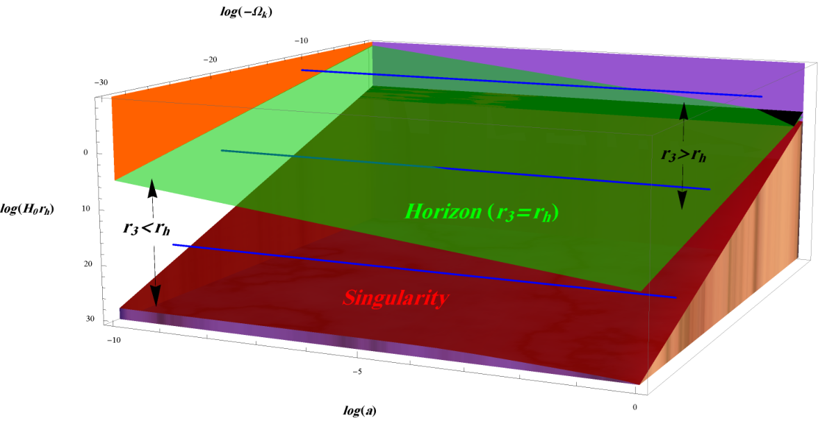
First, note that the figure is plotted for the negative (or normal) branch, which, as discussed above, is physically more relevant. The empirical upper limit for the spatial curvature of the universe (e.g. [20]) is indicated by the purple vertical plane in the figure. The red surface represents those pairs of for which from present time () back to Big Bang Nucleosynthesis (BBN; ). Here we have chosen the empirical bound in (32), and have taken BBN as the earliest constraint on deviations from the standard cosmological model. As we noted before, according to the reality constraint (30) this is the maximum allowed value for at a given time. Therefore the whole area under the red surface is not allowed. Moreover, the red surface also shows the possible choices of the pairs for which the pressure becomes singular for a given . Consequently no pressure singularity could happen for pairs chosen to be above the red plane at any given time.
The green plane indicates those pairs for which the radius of our 4 dimensional universe coincides with the black hole horizon in the 5 dimensional bulk, i.e. . Therefore, for any under the green plane, we have . For those pairs chosen to be above this plane the radius of our holographic universe is larger than the horizon radius, meaning that our present cosmos lies outside the horizon of the black hole in the bulk, i.e. . Subsequently, suppose we choose any pair of above the green plane at the present time (the plane) and move backwards in time. Let us assume that the universe today has its radius larger than the horizon in the bulk black hole. Moving backwards to early times ( plane), as the radius of the universe (proportional to scale factor ) decreases, it may or may not cross the green plane. This has been illustrated with the upper two blue lines in Figure 2, the lower of which pierces the green plane at some value of near .
Indeed, crossing the green plane means that at some early time the radius of the universe was smaller than the horizon radius. Since nothing can escape the horizon of a black hole, one would exclude those pairs of for which their corresponding blue lines at some cross the green plane. Consequently the pairs highlighted with orange plane are possible choices of parameters that satisfy for at .
Consequently, one may interpret the crossing before BBN () as the emergence of the holographic universe out of a “collapsing star”: this scenario replaces the Big Bang singularity. The overall picture of this proposal is shown in the Penrose diagram in Figure (3)-left, which is reminiscent of the core-collapse of a supernova.
Another possibility is to consider a white hole in the bulk rather than a black hole. With this scenario, it is possible for the universe to be inside the horizon at any time up to the present since all matter eventually emerges from the white hole horizon. Therefore the entire range of pairs above the red surface is allowed; the lowest blue line in Figure 2 illustrates one such possible scenario. In this picture one may interpret the pressure singularity as a holographic description of the Big Bang that takes place at . Hence those pairs with satisfying , i.e. lie above the intersection of the red surface and the plane are allowed11 1 We have chosen in (32) and .. For instance, choosing any value for in the range with its corresponding horizon radius, i.e. , represents a holographic universe that emerges from the pressure singularity during the radiation era, passes through the white hole horizon at , and eventually is just outside the horizon at the present time. This is illustrated with a black strip in Figure 2, visible at the upper right of the diagram and continuing underneath the green surface toward the upper left. For any , the universe is inside the horizon at the present time but (given that its expansion is now dominated by the cosmological constant), it will expand indefinitely and eventually intersect the horizon in the future. The overall picture for this scenario has been shown in the Penrose diagram in Figure (3)-right.
From the physical point of view, the former scenario, which we can dub the “black hole” universe is more plausible than the latter “white hole” universe. The reason is that the region inside a white hole horizon is to the future of a 4D white hole naked singularity (Figure 3-right), which makes the brane dynamics, at best contrived, and at worst ill-defined. In particular, it is hard to physically justify why this singularity (i.e. high curvature region) is preceded by a smooth “zero temperature” space-time. For example, it would be in contrast to (and thus more contrived than) the thermal bath that is the outcome of the big bang singularity.
4 Brane Atmosphere and Cosmological Perturbations
In this section, we introduce a mechanism to generate scale-invariant cosmological perturbations in our holographic big bang. As the holographic fluid is sub-dominant for most of the cosmic evolution, one expects the standard cosmological perturbation theory, that has been extremely successful in explaining cosmic microwave background observations (e.g. [1, 20], amongst other observational probes), to be applicable. The fluid will dominate cosmic evolution at very late times, but that can be avoided for sufficiently large or small .
For super horizon perturbations, general arguments based on locality and causality imply that one can use Friedmann equations with independent constants of motion, within independent Hubble patches. In the presence of adiabatic perturbations, which are currently consistent with all cosmological observations (e.g. [1, 20]), these independent Hubble patches would only differ in their local value of comoving spatial curvature . This is often quantified using the Bardeen variable, , where:
| (36) |
or equivalently the comoving gauge linearized metric takes the form
| (37) |
where is a traceless 3-tensor. Planck (+WMAP) observations [20] show that has a near-scale-invariant spectrum of perturbations:
| (38) |
where is the comoving wavenumber for spatial fluctuations.
Given that we assumed (or mirror) boundary conditions for our 3-brane, we can imagine an atmosphere composed of bulk degrees of freedom, which is stratified just outside the 3-brane, due to the gravitational pull of the black hole. Here, we argue that the thermal fluctuations in the atmosphere of the 3-brane induce a near-scale-invariant spectrum of curvature perturbations ( Eq. 38) on our cosmological brane.
Let us first compute the power spectrum of density fluctuations for a thermal gas of massless scalar particles in (4+1)-dimensional flat spacetime. The thermal 2-point correlation function of a free scalar field is given in terms of the Bose-Einstein distribution:
| (39) |
where is the spatial wave-number in 4+1D () , and we used for massless particles. Now, using the definition of energy density:
| (40) |
straightforward manipulations using Eq. (39) yield
| (41) |
Let us next consider how these density fluctuations affect metric fluctuations. As a first attempt, we focus on the linear scalar metric fluctuations in (4+1)-dimensions, which in the longitudinal gauge can be written as:
| (42) |
where is the analog of the Newtonian potential. We can then use 4d Poisson equation to find the statistics of scalar metric fluctuations. Using Eq. (41), we can find the equal-time correlator of :
| (43) |
where
| (44) | |||||
| (45) |
while we have dropped the power-law UV-divergent term ( [cut-off]6), e.g. using dimensional regularization. This UV-divergent term does not depend on temperature, and presumably can be cancelled with appropriate counter-terms in other regularization schemes.
Now, we notice that for small , we have
| (46) |
where is the Riemann zeta function. Therefore, Eq. (43) implies that the 4d Newtonian potential, due to thermal fluctuations, has a scale-invariant power spectrum of the amplitude of .
It is easy to understand this result on dimensional grounds. Looking at the low frequency limit of thermal density fluctuations (41), we notice that the argument inside the absolute value becomes the delta function. In other words, the densities are only correlated within a thermal wavelength , and only have white noise, or a flat power spectrum, on large scales22 2 Note that this is a general feature of Bose-Einstein distributions, on any space-time dimension.. Then, Poisson equation implies that the potential power spectrum scales as , yielding a logarithmic real-space correlation function, or equivalently, a flat dimensionless power spectrum.
So far, all we have done is to study the fluctuations of a statistically uniform 4 dimensional thermal bath. While the scale-invariance of this result is suggestive, it is not immediately clear what this might imply (if anything) for cosmological curvature perturbations on our 3-brane. To answer this question, we will first assume that, at some point in its early cosmological evolution, our 3-brane was in static equilibrium with its thermal 4d atmosphere. Then a comparison of (37) and (42) implies that
| (47) |
assuming boundary conditions at . Note that this boundary condition modifies the thermal spectrum (41) within a thermal wavelength of the 3-brane; given that gravity is a long-range force, we do not expect this to significantly affect the long wave-length metric fluctuations. Therefore, using (47), we can put forth our prediction for the power spectrum of cosmological curvature fluctuations:
| (48) | |||||
where is the temperature of the bulk atmosphere, at the moment of equilibrium, where the scale factor is . Furthermore, we used the definition of 5d Planck mass (2) to substitute for . Comparing Eq. (48) with Eq. (38) gives the experimental constraint on the (effective) temperature of the atmosphere:
| (49) |
for the comoving scale of Mpc-1. While is for the atmosphere in the bulk, based on the rate of change in spatial geometry, we may expect the “de-Sitter” temperature of the boundary to set a minimum for . Therefore, we expect:
| (50) |
The slight deviation from scale-invariance in Eq. (38), which is at the level of 4%, and is now detected with Planck at level, is not predicted in our simple model of thermal free 5D field theory. In the next section, we will speculate on the possible origins of this deviation in our set-up, even though we postpone a full exploration for future study.
5 Summary and Discussions
In the context of DGP brane-world gravity, we have developed a novel holographic perspective on cosmological evolution, which can circumvent a big bang singularity in our past, and produce scale-invariant primordial curvature perturbations, consistent with modern cosmological observations. In this paper, we first provided a pedagogical derivation for the cosmological evolution of DGP braneworld in FRW symmetry from first principles, and then connected it to motion in the Schwarszchild bulk geometry, extending the analyses in [15] to realistic cosmologies. Focusing on the pressure singularity uncovered in [15], we showed that it is generically encountered at early times as matter density decays more slowly than . However, we show that the singularity always happens inside a white hole horizon, and only happens later than Big Bang Nucleosysntheis (BBN) for a small corner of the allowed parameter space (i.e. the base of black strip in Fig. 2). Therefore, it can never be created through evolution from smooth initial conditions. This yields an alternative holographic origin for the big bang, in which our universe emerges from the collapse a 5D “star” into a black hole, reminiscent of an astrophysical core-collapse supernova (Fig. 3-left). In this scenario, there is no big bang singularity in our causal past, and the only singularity is shielded by a black hole horizon. Surprisingly, we found that a thermal atmosphere in equilibrium with the brane can lead to scale-invariant curvature perturbations at the level of cosmological observations, with little fine-tuning, i.e. if the temperature is % of the 5D Planck mass.
We may go further and argue that other problems in standard cosmology, traditionally solved by inflation, can also be addressed in our scenario:
- 1.
The Horizon Problem, which refers to the uniform temperature of causally disconnected patches, is addressed, as the “star” that collapsed into a 5D black hole could have had plenty of time to reach uniform temperature across its core.
- 2.
The Flatness Problem, which refers to the surprisingly small spatial curvature of our universe, is addressed by assuming a large mass/energy for the 5D “star”, . The radius of the black hole horizon, , sets the maximum spatial Ricci curvature (or minimum radius of curvature) for our universe, and thus can only dominate at late times. If one assumes that the initial Hubble constant is the 5D Planck mass, which is supported by the scale of curvature perturbations above, we have , which could become sufficiently small, for massive stars.
The curvature could of course be detectable at late times, as the Hubble constant drops, depending on the scale of dark energy. However, a detection curvature should generically accompany a detection of large scale anisotropy, as a generic black hole will have a finite angular momentum, which would distort FRW symmetry on the scale of the curvature.
- 3.
The Monopole Problem refers to the absence of Grand Unified Theory (GUT) monopoles, that should generically form (and over-close the universe) after the GUT phase transition. As we have replaced the singular big bang, with the emergence of a 4D universe at a finite size, the plasma temperature never reaches GUT scale, and thus the GUT phase transition will never have happened in the thermal history of the universe, preventing copious production of monopoles.
To see this, we can translate the observational constraints on the DGP cosmology (normal branch), [14] into an upper limit on 5D Planck mass:
(51) where we used the inequality in Eq. (50) to bound the Hubble constant. Correspondingly, the upper limit on the temperature comes from the Friedmann equation in the radiation era, for species:
(52)
Yet another attractive feature of our construction is that it lives in an asymptotically flat space-time. This potentially allows for an S-matrix description of this cosmology, through collapse of an ingoing shell, and emergence of outcoming D-brane. This might be a promising avenue, especially in light of significant recent progress in understanding scattering amplitudes in supergravity (e.g. [21, 22]. Furthermore, with trivial modification, this model could also be embedded in an AdS bulk, which can potentially allow a study of the strongly-coupled dynamics of emergence through AdS/CFT correspondence. Since embedding our braneworld in a large AdS space-time (instead of Minkowski) simply amounts to adding a small constant to the right hand side of e.g., Eqs. (8) or (14), it need not significantly change any of the quantitative results that we have found here.
Let us now comment on (some) potential problems. Perhaps the most notable problem with the DGP model might be the claim [23] that superluminal propagation around non-trivial backgrounds in DGP model hinders causal evolution, and UV analyticity/completion. However this violation of causality is only a pathology for spacetimes that don’t admit a consistent chronology for (super)luminal signals [24]. Such spacetimes, e.g. Godel metric, even exist in General Relativity, and simply point out the absence of global causal evolution in those backgrounds. Therefore such geometries cannot emerge out of classical causal evolution. The second objection is more subtle, and relies on the analyticity properties of the scattering amplitudes for the DGP scalar. However, these conditions (e.g. the Froissart bound) may be violated in the presence of massless bulk gravitons. Therefore, these arguments would leave the door open for a possible UV completion via e.g. string theory and/or AdS/CFT correspondence.
Another possible pathology of the DGP model is copious spontaneous production of self-accelerating branes in the bulk [15], which is estimated via Euclidean instanton methods. However one may argue that, since self-accelerating branches have catastrophic ghost instabilities, they should be excised (or exorcised) from the Hilbert space of the system. Given that one cannot classically transition from the normal branch to the self-accelerating branch, this modification would not affect the semi-classical behavior, but would prevent tunnelling into unphysical states.
Finally, let us comment on potential testability of this model. As we pointed out, the simple model of cosmological perturbations, developed in Sec. 4 is already ruled out by cosmological observations at level, as it does not predict any deviations from scale-invariance. However, it is easy to imagine small corrections that could lead to a deviation from scale-invariance, especially given that bulk temperature is so close (i.e. of) the 5D Planck temperature. In the context of our model, the red tilt of the cosmological power spectrum implies that the amplitude of 5D bulk graviton propagator, which enters in Eq. (43), is getting stronger in the IR, suggesting gradual unfreezing of additional polarizations of graviton. For example, this is what one would expect in cascading gravity [25], where DGP bulk is replaced by a 4-brane, which is itself embedded in a 6D bulk. Similar to the ordinary DGP, the transition in flat space happens on length-scales larger than , as the scalar field associated with the motion of the 4-brane in the 6D bulk becomes weakly coupled, and boosts the strength of the gravitational exchange amplitude.
A related issue is that the gravitational Jeans instability of the thermal atmosphere kicks in for , which may appear to limit the range of scale-invariant power spectrum to less than the current observations. However, the time-scale for the Jeans instability can be significantly longer than the Hubble time, thus limiting its maximum growth. Nevertheless, one may consider the residual Jeans instability as a potential origin for the slight red tilt (i.e. ) of the observed power spectrum. We defer a consistent inclusion of gravitational backreaction on the 5d thermal power spectrum (which should account for the impact of Jeans instability) to a future study.
We should stress that, at this point, the development of a mechanism responsible for the observed deviation from scale-invariance is the most immediate phenomenological challenge for our scenario. The next challenge would be a study of the interactions that lead to deviations from scale-invariance, and whether they satisfy the stringent observational bounds on primordial non-gaussianity [26]. Other interesting questions might be, given that the emergence from the 5D black hole might happen at relatively low temperatures, could there be observable predictions for gravitational waves (either on cosmological scales, or for gravitational wave interferometers), or even modifications of light element abundances in Big Bang Nucleosynthesis.
Ultimately, an entire new world might emerge “Out of the White Hole”, and replace Big Bang with a mere mirage of a non-existent past!
Acknowledgements We would like to thank Nima Doroud, Gregory Gabadadze, Ruth Gregory, Rob Myers, Paul McFadden, Eric Poisson, Kostas Skenderis, Misha Smolkin, Marika Taylor and Herman Verlinde for inspiring discussions and useful comments. This work was supported by the Natural Science and Engineering Research Council of Canada, the University of Waterloo and by Perimeter Institute for Theoretical Physics. Research at Perimeter Institute is supported by the Government of Canada through Industry Canada and by the Province of Ontario through the Ministry of Research & Innovation.
References
- (1) Planck Collaboration Collaboration, P. Ade et al., Planck 2013 results. I. Overview of products and scientific results, arXiv:1303.5062.
- (2) L. Randall and R. Sundrum, A Large mass hierarchy from a small extra dimension, Phys.Rev.Lett. 83 (1999) 3370–3373, [hep-ph/9905221].
- (3) H. Collins and B. Holdom, Brane cosmologies without orbifolds, Phys.Rev. D62 (2000) 105009, [hep-ph/0003173].
- (4) G. Dvali, G. Gabadadze, and M. Porrati, 4-D gravity on a brane in 5-D Minkowski space, Phys.Lett. B485 (2000) 208–214, [hep-th/0005016].
- (5) A. Vainshtein, To the problem of nonvanishing gravitation mass, Phys.Lett. B39 (1972) 393–394.
- (6) I. Savonije and E. P. Verlinde, CFT and entropy on the brane, Phys.Lett. B507 (2001) 305–311, [hep-th/0102042].
- (7) S. S. Gubser, AdS / CFT and gravity, Phys.Rev. D63 (2001) 084017, [hep-th/9912001].
- (8) L. Pilo, R. Rattazzi, and A. Zaffaroni, The Fate of the radion in models with metastable graviton, JHEP 0007 (2000) 056, [hep-th/0004028].
- (9) M. A. Luty, M. Porrati, and R. Rattazzi, Strong interactions and stability in the DGP model, JHEP 0309 (2003) 029, [hep-th/0303116].
- (10) A. Nicolis and R. Rattazzi, Classical and quantum consistency of the DGP model, JHEP 0406 (2004) 059, [hep-th/0404159].
- (11) C. Charmousis, R. Gregory, N. Kaloper, and A. Padilla, DGP Specteroscopy, JHEP 0610 (2006) 066, [hep-th/0604086].
- (12) N. Kaloper, Gravitational shock waves and their scattering in brane-induced gravity, Phys.Rev. D71 (2005) 086003, [hep-th/0502035].
- (13) W. Fang, S. Wang, W. Hu, Z. Haiman, L. Hui, et al., Challenges to the DGP Model from Horizon-Scale Growth and Geometry, Phys.Rev. D78 (2008) 103509, [arXiv:0808.2208].
- (14) T. Azizi, M. Sadegh Movahed, and K. Nozari, Observational Constraints on the Normal Branch of a Warped DGP Cosmology, New Astron. 17 (2012) 424–432, [arXiv:1111.3195].
- (15) R. Gregory, N. Kaloper, R. C. Myers, and A. Padilla, A New perspective on DGP gravity, JHEP 0710 (2007) 069, [arXiv:0707.2666].
- (16) J. D. Brown and J. York, James W., Quasilocal energy and conserved charges derived from the gravitational action, Phys.Rev. D47 (1993) 1407–1419, [gr-qc/9209012].
- (17) K.-i. Maeda, S. Mizuno, and T. Torii, Effective gravitational equations on brane world with induced gravity, Phys.Rev. D68 (2003) 024033, [gr-qc/0303039].
- (18) L. Susskind, The World as a hologram, J.Math.Phys. 36 (1995) 6377–6396, [hep-th/9409089].
- (19) C. Deffayet, Cosmology on a brane in Minkowski bulk, Phys.Lett. B502 (2001) 199–208, [hep-th/0010186].
- (20) Planck Collaboration Collaboration, P. Ade et al., Planck 2013 results. XVI. Cosmological parameters, arXiv:1303.5076.
- (21) F. Cachazo and Y. Geyer, A ’Twistor String’ Inspired Formula For Tree-Level Scattering Amplitudes in N=8 SUGRA, arXiv:1206.6511.
- (22) F. Cachazo, L. Mason, and D. Skinner, Gravity in Twistor Space and its Grassmannian Formulation, arXiv:1207.4712.
- (23) A. Adams, N. Arkani-Hamed, S. Dubovsky, A. Nicolis, and R. Rattazzi, Causality, analyticity and an IR obstruction to UV completion, JHEP 0610 (2006) 014, [hep-th/0602178].
- (24) J.-P. Bruneton, On causality and superluminal behavior in classical field theories: Applications to k-essence theories and MOND-like theories of gravity, Phys.Rev. D75 (2007) 085013, [gr-qc/0607055].
- (25) C. de Rham, G. Dvali, S. Hofmann, J. Khoury, O. Pujolas, et al., Cascading gravity: Extending the Dvali-Gabadadze-Porrati model to higher dimension, Phys.Rev.Lett. 100 (2008) 251603, [arXiv:0711.2072].
- (26) Planck Collaboration Collaboration, P. Ade et al., Planck 2013 Results. XXIV. Constraints on primordial non-Gaussianity, arXiv:1303.5084.