跳到论文正文
W Papers独立论文阅读器 arXiv:1309.1225 论文正文 计算阅读时间 · 0%
引用这篇论文根据当前论文元数据生成,正式投稿前建议核对。


License: arXiv.org perpetual non-exclusive license
arXiv:1309.1225v2 [math.AP] 13 Sep 2014

Random data Cauchy theory for nonlinear wave equations of power-type on ℝ3{\mathbb{R}}^{3}Thanks: 2010 Mathematics Subject Classification. 35L05, 35R60, 35Q55Thanks: Key words and phrases. nonlinear wave equation; almost sure global well-posedness; random initial dataThanks: The first author was supported in part by the Swiss National Science Foundation under grant SNF 200021-140467. The second author was supported in part by the U.S. National Science Foundation grant DMS-1068815 and by the NSERC Postgraduate Scholarships Program

Jonas Lührmann Address: Departement Mathematik
ETH Zürich
8092 Zürich
Switzerland
Email address: jonas.luehrmann@math.ethz.ch
and Dana Mendelson Address: Department of Mathematics
Massachusetts Institute of Technology
77 Massachusetts Ave
Cambridge, MA 02139
USA
Email address: dana@math.mit.edu
Abstract.

We consider the defocusing nonlinear wave equation of power-type on ℝ3{\mathbb{R}}^{3}. We establish an almost sure global existence result with respect to a suitable randomization of the initial data. In particular, this provides examples of initial data of super-critical regularity which lead to global solutions. The proof is based upon Bourgain’s high-low frequency decomposition and improved averaging effects for the free evolution of the randomized initial data.

1. Introduction

We consider the Cauchy problem for the defocusing nonlinear wave equation

(1.1) {−ut​t+Δ​u=|u|ρ−1​u​ on ​ℝ×ℝ3,(u,ut)|t=0=(f1,f2)∈Hxs​(ℝ3)×Hxs−1​(ℝ3),\left\{\begin{split}-u_{tt}+\Delta u&=|u|^{\rho-1}u\text{ on }{\mathbb{R}}\times{\mathbb{R}}^{3},\\ (u,u_{t})|_{t=0}&=(f_{1},f_{2})\in H^{s}_{x}({\mathbb{R}}^{3})\times H^{s-1}_{x}({\mathbb{R}}^{3}),\end{split}\right.

where 3≤ρ≤53\leq\rho\leq 5 and Hxs​(ℝ3)H^{s}_{x}({\mathbb{R}}^{3}) is the usual inhomogeneous Sobolev space. The main result of this paper establishes the almost sure existence of global solutions to (1.1) with respect to a suitable randomization of initial data in Hxs​(ℝ3)×Hxs−1​(ℝ3)H^{s}_{x}({\mathbb{R}}^{3})\times H^{s-1}_{x}({\mathbb{R}}^{3}) for 3≤ρ<53\leq\rho<5 and ρ3+5​ρ2−11​ρ−39​ρ2−6​ρ−3<s<1\frac{\rho^{3}+5\rho^{2}-11\rho-3}{9\rho^{2}-6\rho-3}<s<1. In particular, for 14​(7+73)<ρ<5\frac{1}{4}(7+\sqrt{73})<\rho<5, this yields examples of initial data of super-critical regularity for which solutions to (1.1) exist globally in time. See Remark 4.3 for a discussion of uniqueness of these solutions.

A systematic investigation of the local well-posedness of (1.1) for initial data in homogeneous Sobolev spaces is undertaken by Lindblad and Sogge in [24], where local strong solutions to (1.1) are constructed for s≥32−2ρ−1s\geq\frac{3}{2}-\frac{2}{\rho-1} using Strichartz estimates for the wave equation. When s<32−2ρ−1s<\frac{3}{2}-\frac{2}{\rho-1}, this is the super-critical regime and the well-posedness arguments based on Strichartz estimates break down. Recently, several methods have emerged proving ill-posedness for (1.1) below the critical scaling regularity (see Lebeau [22], Christ-Colliander-Tao [13] and Ibrahim-Majdoub-Masmoudi [19]).

Nevertheless, using probabilistic tools, it has been possible to construct large sets of initial data of super-critical regularity that lead to unique local and even global solutions to several nonlinear dispersive equations. This approach was initiated by Bourgain [4, 5] for the periodic nonlinear Schrödinger equation in one and two space dimensions. Building upon work by Lebowitz, Rose and Speer [23], Bourgain proved the invariance of the Gibbs measure under the flow of the equation and used this invariance to prove almost sure global well-posedness in the support of the measure. In [10, 11], Burq and Tzvetkov consider the cubic nonlinear wave equation on a three-dimensional compact manifold. They construct large sets of initial data of super-critical regularity that lead to local solutions via a randomization procedure which relies on expansion of the initial data with respect to an orthonormal basis of eigenfunctions of the Laplacian. Together with invariant measure considerations they also prove almost sure global existence for the cubic nonlinear wave equation on the three-dimensional unit ball. Many further results in this direction have been obtained in recent years (see [40], [41], [9], [39], [28], [25], [27], [34], [7] and references therein).

Although it is desirable to establish the existence of an invariant Gibbs measure, in many situations there are serious technical difficulties associated with defining such a measure. In the absence of an invariant measure, other approaches have been developed to show almost sure global existence for periodic super-critical equations via a suitable randomization of the initial data. Energy estimates are used by Nahmod, Pavlović and Staffilani [26] in the context of the periodic Navier-Stokes equation in two and three dimensions and by Burq and Tzvetkov for the three-dimensional periodic defocusing cubic nonlinear wave equation. Colliander and Oh [14] adapt Bourgain’s high-low frequency decomposition [6] to prove almost sure global existence of solutions to the one-dimensional periodic defocusing cubic nonlinear Schrödinger equation below L2​(𝕋)L^{2}(\mathbb{T}).

In this work we study almost sure global existence for nonlinear wave equations on Euclidean space without any radial symmetry assumption on the initial data. Previous results on Euclidean space have involved first considering a related equation in a setting where an orthonormal basis of eigenfunctions of the Laplacian exists. This orthonormal basis is used to randomize the initial data for the related equation and an appropriate transform is then used to map solutions of the related equation to solutions of the original equation. Burq, Thomann and Tzvetkov [8, Theorem 1.2] prove almost sure global existence and scattering for the defocusing nonlinear Schrödinger equation on ℝ{\mathbb{R}} by first treating a one-dimensional nonlinear Schrödinger equation with a harmonic potential and then invoking the lens transform [8, (10.2)]. Subsequently, similar approaches were used by Deng [15, Theorem 1.2], Poiret [32], [31] and Poiret, Robert and Thomann [33, Theorem 1.3] to study the defocusing nonlinear Schrödinger equation on ℝd{\mathbb{R}}^{d} for d≥2d\geq 2. In the context of the wave equation, Suzzoni [36], [37, Theorem 1.2] first considers a nonlinear wave equation on the three-dimensional sphere and then uses the Penrose transform [36, (3)] to obtain almost sure global existence and scattering for (1.1) for 3≤ρ<43\leq\rho<4.

Instead of using such transforms, we will randomize functions directly on Euclidean space via a unit-scale decomposition in frequency space. More precisely, let φ∈Cc∞​(ℝ3)\varphi\in C_{c}^{\infty}({\mathbb{R}}^{3}) be a real-valued, smooth, non-increasing function such that 0≤φ≤10\leq\varphi\leq 1 and

φ(ξ)={1for ​|ξ|≤1,0for ​|ξ|≥2.\varphi(\xi)=\left\{\begin{split}&1\qquad\text{for }|\xi|\leq 1,\\ &0\qquad\text{for }|\xi|\geq 2.\end{split}\right.

For every k∈ℤ3k\in{\mathbb{Z}}^{3} set φk​(ξ)=φ⁡(ξ−k)\varphi_{k}(\xi)=\varphi(\xi-k) and define

ψk​(ξ)=φk​(ξ)∑l∈ℤ3φl​(ξ).\psi_{k}(\xi)=\frac{\varphi_{k}(\xi)}{\sum_{l\in{\mathbb{Z}}^{3}}\varphi_{l}(\xi)}.

Then ψk\psi_{k} is smooth with support contained in {ξ∈ℝ3:|ξ−k|≤2}\{\xi\in{\mathbb{R}}^{3}:|\xi-k|\leq 2\}. Note that ∑k∈ℤ3ψk​(ξ)=1\sum_{k\in{\mathbb{Z}}^{3}}\psi_{k}(\xi)=1 for all ξ∈ℝ3\xi\in{\mathbb{R}}^{3}. For f∈Lx2​(ℝ3)f\in L^{2}_{x}({\mathbb{R}}^{3}) define the function Pk​f:ℝ3→ℂP_{k}f:{\mathbb{R}}^{3}\rightarrow{\mathbb{C}} by

(Pk​f)​(x)=ℱ−1​(ψk​(ξ)​f^​(ξ))​(x)​ for ​x∈ℝ3.(P_{k}f)(x)={\mathcal{F}}^{-1}\left(\psi_{k}(\xi)\hat{f}(\xi)\right)(x)\text{ for }x\in{\mathbb{R}}^{3}.

If f∈Hxs​(ℝ3)f\in H^{s}_{x}({\mathbb{R}}^{3}) for some s∈ℝs\in{\mathbb{R}}, then Pk​f∈Hxs​(ℝ3)P_{k}f\in H^{s}_{x}({\mathbb{R}}^{3}) and f=∑k∈ℤ3Pk​f​ in ​Hxs​(ℝ3)f=\sum_{k\in{\mathbb{Z}}^{3}}P_{k}f\text{ in }H^{s}_{x}({\mathbb{R}}^{3}) with

(1.2) ‖f‖Hxs​(ℝ3)∼(∑k∈ℤ3‖Pk​f‖Hxs​(ℝ3)2)1/2.\|f\|_{H^{s}_{x}({\mathbb{R}}^{3})}\sim\bigl(\sum_{k\in{\mathbb{Z}}^{3}}\|P_{k}f\|^{2}_{H^{s}_{x}({\mathbb{R}}^{3})}\bigr)^{1/2}.

In the proof of the almost sure existence of global solutions to (1.1), we will crucially exploit that these projections satisfy a unit-scale Bernstein inequality, namely that for all 2≤p1≤p2≤∞2\leq p_{1}\leq p_{2}\leq\infty there exists C≡C⁡(p1,p2)>0C\equiv C(p_{1},p_{2})>0 such that for all f∈Lx2​(ℝ3)f\in L^{2}_{x}({\mathbb{R}}^{3}) and for all k∈ℤ3k\in{\mathbb{Z}}^{3}

(1.3) ‖Pk​f‖Lxp2​(ℝ3)≤C​‖Pk​f‖Lxp1​(ℝ3).\displaystyle\|P_{k}f\|_{L^{p_{2}}_{x}({\mathbb{R}}^{3})}\leq C\|P_{k}f\|_{L^{p_{1}}_{x}({\mathbb{R}}^{3})}.

For a formal statement of this inequality, see Lemma 2.1. Let now {(hk,lk)}k∈ℤ3\{(h_{k},l_{k})\}_{k\in{\mathbb{Z}}^{3}} be a sequence of independent, zero-mean, real-valued random variables on a probability space (Ω,𝒜,ℙ)(\Omega,{\mathcal{A}},{\mathbb{P}}) with distributions μk\mu_{k} and νk\nu_{k}. Assume that there exists c>0c>0 such that

(1.4) |∫−∞+∞eγ​x​d​μk​(x)|≤ec​γ2​ for all ​γ∈ℝ​ and for all ​k∈ℤ3,\left|\int_{-\infty}^{+\infty}e^{\gamma x}\,d\mu_{k}(x)\right|\leq e^{c\gamma^{2}}\text{ for all }\gamma\in{\mathbb{R}}\text{ and for all }k\in{\mathbb{Z}}^{3},

and similarly for νk\nu_{k}. The assumption (1.4) is satisfied, for example, by standard Gaussian random variables, standard Bernoulli random variables, or any random variables with compactly supported distributions. For a given f=(f1,f2)∈Hxs​(ℝ3)×Hxs−1​(ℝ3)f=(f_{1},f_{2})\in H^{s}_{x}({\mathbb{R}}^{3})\times H^{s-1}_{x}({\mathbb{R}}^{3}) we define its randomization by

(1.5) fω=(f1ω,f2ω):=(∑k∈ℤ3hk​(ω)​Pk​f1,∑k∈ℤ3lk​(ω)​Pk​f2).f^{\omega}=(f_{1}^{\omega},f_{2}^{\omega}):=\biggl(\sum_{k\in{\mathbb{Z}}^{3}}h_{k}(\omega)P_{k}f_{1},\sum_{k\in{\mathbb{Z}}^{3}}l_{k}(\omega)P_{k}f_{2}\biggr).

The quantity ∑k∈ℤ3hk​(ω)​Pk​f1\sum_{k\in{\mathbb{Z}}^{3}}h_{k}(\omega)P_{k}f_{1} is understood as the Cauchy limit in L2​(Ω,Hxs​(ℝ3))L^{2}(\Omega;H^{s}_{x}({\mathbb{R}}^{3})) of the sequence (∑|k|≤Nhk​(ω)​Pk​f1)N∈ℕ\Bigl(\sum_{|k|\leq N}h_{k}(\omega)P_{k}f_{1}\Bigr)_{N\in{\mathbb{N}}} and similarly for ∑k∈ℤ3lk​(ω)​Pk​f2\sum_{k\in{\mathbb{Z}}^{3}}l_{k}(\omega)P_{k}f_{2}. Let

(1.6) ufω=cos⁡(t​|∇|)​f1ω+sin⁡(t​|∇|)|∇|​f2ω\displaystyle u_{f}^{\omega}=\cos(t|\nabla|)f_{1}^{\omega}+\frac{\sin(t|\nabla|)}{|\nabla|}f_{2}^{\omega}

be the free wave evolution of the initial data fωf^{\omega} defined in (1.5).

In the case of random variables such that there exists c>0c>0 for which their distributions satisfy

supk∈ℤ3μk​([−c,c])<1,\sup_{k\in{\mathbb{Z}}^{3}}\mu_{k}([-c,c])<1,

one can show that if ff does not belong to Hxs+ε​(ℝ3)×Hxs−1+ε​(ℝ3)H^{s+\varepsilon}_{x}({\mathbb{R}}^{3})\times H^{s-1+\varepsilon}_{x}({\mathbb{R}}^{3}), then the probability that fωf^{\omega} belongs to Hxs+ε​(ℝ3)×Hxs−1+ε​(ℝ3)H^{s+\varepsilon}_{x}({\mathbb{R}}^{3})\times H^{s-1+\varepsilon}_{x}({\mathbb{R}}^{3}) is zero. This follows by a similar argument to the one found in Appendix B of [10], using (1.2). Thus, our randomization procedure does not regularize at the level of Sobolev spaces.

We note that a similar randomization procedure on Euclidean space was used by Zhang and Fang in [42, (1.12)] to study random data local existence and small data global existence questions for the generalized incompressible Navier-Stokes equation on ℝd{\mathbb{R}}^{d} for d≥3d\geq 3.

We are now in a position to state our results.

Theorem 1.1.

Let 3≤ρ<53\leq\rho<5 and let

ρ3+5​ρ2−11​ρ−39​ρ2−6​ρ−3<s<1.\frac{\rho^{3}+5\rho^{2}-11\rho-3}{9\rho^{2}-6\rho-3}<s<1.

Let f=(f1,f2)∈Hxs​(ℝ3)×Hxs−1​(ℝ3)f=(f_{1},f_{2})\in H^{s}_{x}({\mathbb{R}}^{3})\times H^{s-1}_{x}({\mathbb{R}}^{3}). Let {(hk,lk)}k∈ℤ3\{(h_{k},l_{k})\}_{k\in{\mathbb{Z}}^{3}} be a sequence of independent, zero-mean value, real-valued random variables on a probability space (Ω,𝒜,ℙ)(\Omega,{\mathcal{A}},{\mathbb{P}}) with distributions μk\mu_{k} and νk\nu_{k}. Assume that there exists c>0c>0 such that

|∫−∞+∞eγ​x​d​μk​(x)|≤ec​γ2​ for all ​γ∈ℝ​ and for all ​k∈ℤ3\left|\int_{-\infty}^{+\infty}e^{\gamma x}d\mu_{k}(x)\right|\leq e^{c\gamma^{2}}\text{ for all }\gamma\in{\mathbb{R}}\text{ and for all }k\in{\mathbb{Z}}^{3}

and similarly for νk\nu_{k}. Let fω=(f1ω,f2ω)f^{\omega}=(f_{1}^{\omega},f_{2}^{\omega}) be the associated randomized initial data as defined in (1.5) and let ufωu_{f}^{\omega} be the associated free evolution as defined in (1.6). For almost every ω∈Ω\omega\in\Omega there exists a unique global solution

(u,ut)∈(ufω,∂tufω)+C⁡(ℝ,Hx1​(ℝ3)×Lx2​(ℝ3))(u,u_{t})\in(u_{f}^{\omega},\partial_{t}u_{f}^{\omega})+C\bigl({\mathbb{R}};H^{1}_{x}({\mathbb{R}}^{3})\times L^{2}_{x}({\mathbb{R}}^{3})\bigr)

to the nonlinear wave equation

(1.7) {−ut​t+Δ​u=|u|ρ−1​u​ on ​ℝ×ℝ3,(u,ut)|t=0=(f1ω,f2ω).\left\{\begin{split}-u_{tt}+\Delta u&=|u|^{\rho-1}u\text{ on }{\mathbb{R}}\times{\mathbb{R}}^{3},\\ (u,u_{t})|_{t=0}&=(f_{1}^{\omega},f_{2}^{\omega}).\end{split}\right.

Here, uniqueness only holds in a mild sense; see Remark 4.3.

The proof of Theorem 1.1 combines a probabilistic local existence argument with Bourgain’s high-low frequency decomposition [6], an approach introduced by Colliander and Oh [14, Theorem 2] to show almost sure global existence of the one-dimensional periodic defocusing cubic nonlinear Schrödinger equation below L2​(𝕋)L^{2}({\mathbb{T}}). The high-low method was previously used by Kenig, Ponce and Vega [21, Theorem 1.2] to prove global well-posedness of (1.1) for 2≤ρ<52\leq\rho<5 for initial data in a range of sub-critical spaces below the energy space (see also [1], [16] and [35] for ρ=3\rho=3). We adopt arguments from [21].

Theorem 1.1 permits initial data at lower regularities than the deterministic result [21, Theorem 1.2]. This is mainly due to so-called averaging effects for the free evolution of randomized initial data (see Lemma 3.3 below), which are proven by combining the unit-scale Bernstein estimate (1.3) and Strichartz estimates for the wave equation on ℝ3{\mathbb{R}}^{3}. In particular, we use here that the randomization is performed directly on Euclidean space.

Remark 1.2.

For 3≤ρ<43\leq\rho<4, random data Cauchy theory for the nonlinear wave equation (1.1) on ℝ3{\mathbb{R}}^{3} has been addressed by Suzzoni [36, 37] using different approaches than in the proof of Theorem 1.1. In [36, Theorem 2], using methods from [10, 11], almost sure global existence and scattering for (1.1) for 3≤ρ<43\leq\rho<4 is established for radially symmetric initial data in a class of spaces of super-critical regularity related to the Penrose transform. For ρ=3\rho=3, almost sure global existence and scattering for (1.1) is proven in [37, Theorem 1.2], using methods from [12]. In both these cases, the spaces for the initial data do not coincide with Hxs​(ℝ3)×Hxs−1​(ℝ3)H^{s}_{x}({\mathbb{R}}^{3})\times H^{s-1}_{x}({\mathbb{R}}^{3}). We do not address the question of scattering of the constructed solutions in Theorem 1.1. The main difficulty is that the high-low method does not yield bounds on any global space-time norm of the nonlinear component of the solution uu.

Remark 1.3.

During the final revision of this article, the preprints [2, 3] by Bényi-Oh-Pocovnicu and [30] by Pocovnicu appeared which use a similar randomization procedure. In [2, 3] almost sure well-posedness results are established for the cubic nonlinear Schrödinger equation on ℝd\mathbb{R}^{d} for d≥3d\geq 3. In [30] almost sure global well-posedness is proven for the energy-critical defocusing nonlinear wave equation on ℝd\mathbb{R}^{d} for d=4,5d=4,5.

Remark 1.4.

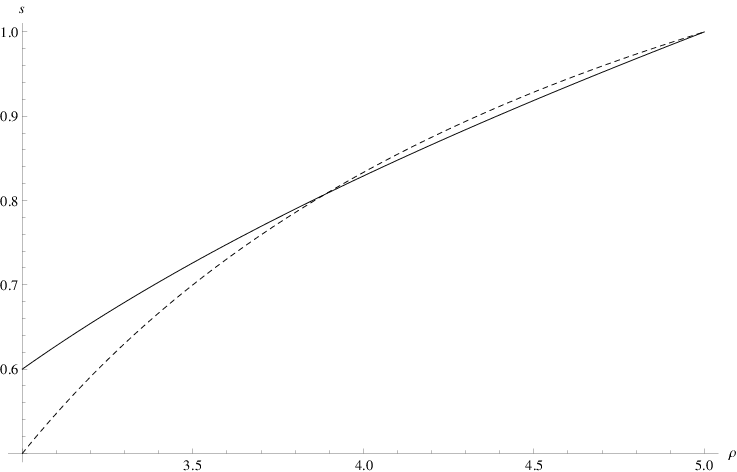
For 14​(7+73)≈3.89<ρ<5\frac{1}{4}(7+\sqrt{73})\approx 3.89<\rho<5, the range of allowable regularity exponents ss in Theorem 1.1 contains super-critical exponents; see Figure 1. To the best of the authors’ knowledge, for 4≤ρ<54\leq\rho<5, Theorem 1.1 is the first result which establishes the existence of large sets of initial data of super-critical regularity which lead to global solutions to (1.1).
Refer to caption
Figure 1. The dashed line is the critical regularity sc=32−2ρ−1s_{c}=\frac{3}{2}-\frac{2}{\rho-1}. The solid line is the threshold for the exponent ss in Theorem 1.1.
Remark 1.5.

For the specific case ρ=3\rho=3, we note that our randomization procedure allows us to straightforwardly adapt the proofs in [12] to the Euclidean setting. In particular, by modifying the proof of the averaging effects of Corollary A.4 of [12], we can use the arguments of Proposition 2.1 and Proposition 2.2 of [12] to prove that if 0<s<10<s<1 and f=(f1,f2)∈Hxs​(ℝ3)×Hxs−1​(ℝ3)f=(f_{1},f_{2})\in H^{s}_{x}({\mathbb{R}}^{3})\times H^{s-1}_{x}({\mathbb{R}}^{3}), then for almost every ω∈Ω\omega\in\Omega there exists a unique global solution

(u,ut)∈(ufω,∂tufω)+C⁡(ℝ,Hx1​(ℝ3)×Lx2​(ℝ3))(u,u_{t})\in(u_{f}^{\omega},\partial_{t}u_{f}^{\omega})+C\bigl({\mathbb{R}};H^{1}_{x}({\mathbb{R}}^{3})\times L^{2}_{x}({\mathbb{R}}^{3})\bigr)

to the defocusing cubic nonlinear wave equation on ℝ3{\mathbb{R}}^{3} with initial data fωf^{\omega}. This is an improvement over the corresponding range 35<s<1\frac{3}{5}<s<1 in Theorem 1.1. In contrast, these arguments which proceed via energy estimates cannot be applied directly in the case 3<ρ<53<\rho<5. In such an argument, one would need bounds on ‖|u|ρ−1​u‖Lt1​Lx2​(ℝ×ℝ3)=‖u‖Ltρ​Lx2​ρ​(ℝ×ℝ3)ρ\||u|^{\rho-1}u\|_{L_{t}^{1}L_{x}^{2}({\mathbb{R}}\times{\mathbb{R}}^{3})}=\|u\|^{\rho}_{L_{t}^{\rho}L_{x}^{2\rho}({\mathbb{R}}\times{\mathbb{R}}^{3})} but one no longer has the necessary Sobolev embedding to close the argument.

When ρ=5\rho=5, the nonlinear wave equation (1.1) is energy-critical and the high-low argument no longer works. However, by establishing probabilistic a priori estimates on the Lt5​Lx10​(ℝ×ℝ3)L^{5}_{t}L^{10}_{x}({\mathbb{R}}\times{\mathbb{R}}^{3}) norm of the free evolution ufωu_{f}^{\omega}, we obtain the following probabilistic small data global existence result.

Theorem 1.6.

Let 25≤s<1\frac{2}{5}\leq s<1 and f=(f1,f2)∈Hxs​(ℝ3)×H˙xs−1​(ℝ3)f=(f_{1},f_{2})\in H^{s}_{x}({\mathbb{R}}^{3})\times\dot{H}^{s-1}_{x}({\mathbb{R}}^{3}). Let {(hk,lk)}k∈ℤ3\{(h_{k},l_{k})\}_{k\in{\mathbb{Z}}^{3}} be a sequence of independent, zero-mean value, real-valued random variables on a probability space (Ω,𝒜,ℙ)(\Omega,{\mathcal{A}},{\mathbb{P}}) with distributions μk\mu_{k} and νk\nu_{k}. Assume that there exists c>0c>0 such that

|∫−∞+∞eγ​x​d​μk​(x)|≤ec​γ2​ for all ​γ∈ℝ​ and for all ​k∈ℤ3\left|\int_{-\infty}^{+\infty}e^{\gamma x}d\mu_{k}(x)\right|\leq e^{c\gamma^{2}}\text{ for all }\gamma\in{\mathbb{R}}\text{ and for all }k\in{\mathbb{Z}}^{3}

and similarly for νk\nu_{k}. Let fω=(f1ω,f2ω)f^{\omega}=(f_{1}^{\omega},f_{2}^{\omega}) be the associated randomized initial data as defined in (1.5) and let ufωu_{f}^{\omega} be the associated free evolution as defined in (1.6). There exists Ωf⊂Ω\Omega_{f}\subset\Omega with

(1.8) ℙ(Ωf)≥1−Ce−c/∥f∥2Hxs×H˙xs−1{\mathbb{P}}(\Omega_{f})\geq 1-Ce^{-c/\|f\|^{2}_{H^{s}_{x}\times\dot{H}^{s-1}_{x}}}

for some absolute constants C,c>0C,c>0, such that for every ω∈Ωf\omega\in\Omega_{f} there exists a unique global solution

(u,ut)∈(ufω,∂tufω)+C⁡(ℝ,H˙x1​(ℝ3)×Lx2​(ℝ3))(u,u_{t})\in(u_{f}^{\omega},\partial_{t}u_{f}^{\omega})+C\bigl({\mathbb{R}};\dot{H}^{1}_{x}({\mathbb{R}}^{3})\times L^{2}_{x}({\mathbb{R}}^{3})\bigr)

to the quintic nonlinear wave equation

(1.9) {−ut​t+Δ​u=|u|4​u​ on ​ℝ×ℝ3,(u,ut)|t=0=(f1ω,f2ω).\left\{\begin{split}-u_{tt}+\Delta u&=|u|^{4}u\text{ on }{\mathbb{R}}\times{\mathbb{R}}^{3},\\ (u,u_{t})|_{t=0}&=(f_{1}^{\omega},f_{2}^{\omega}).\end{split}\right.

Moreover, we have scattering in the sense that for every ω∈Ωf\omega\in\Omega_{f} there exist (v1,v2)∈H˙x1​(ℝ3)×Lx2​(ℝ3)(v_{1},v_{2})\in\dot{H}^{1}_{x}({\mathbb{R}}^{3})\times L^{2}_{x}({\mathbb{R}}^{3}) such that the free evolution v⁡(t)=cos⁡(t​|∇|)​v1+sin⁡(t​|∇|)|∇|​v2v(t)=\cos(t|\nabla|)v_{1}+\frac{\sin(t|\nabla|)}{|\nabla|}v_{2} satisfies

‖(u⁡(t)−ufω​(t)−v⁡(t),∂tu⁡(t)−∂tufω​(t)−∂tv⁡(t))‖H˙x1​(ℝ3)×Lx2​(ℝ3)⟶0​ as ​t→±∞.\bigl\|\bigl(u(t)-u_{f}^{\omega}(t)-v(t),\partial_{t}u(t)-\partial_{t}u_{f}^{\omega}(t)-\partial_{t}v(t)\bigr)\bigr\|_{\dot{H}^{1}_{x}({\mathbb{R}}^{3})\times L^{2}_{x}({\mathbb{R}}^{3})}\longrightarrow 0\text{ as }t\rightarrow\pm\infty.
Remark 1.7.

We note that the statement is only meaningful if

‖f‖Hxs×H˙xs−1≤(clog⁡(C))1/2,\|f\|_{H^{s}_{x}\times\dot{H}^{s-1}_{x}}\leq\left(\frac{c}{\log(C)}\right)^{1/2},

which reflects that Theorem 1.6 is a small data result.

Notation: We let C>0C>0 denote a constant that depends only on fixed parameters and whose value may change from line to line. We write X≲YX\lesssim Y to denote X≤C​YX\leq CY for some C>0C>0. As mentioned above, Hxs​(ℝ3)H^{s}_{x}({\mathbb{R}}^{3}) denotes the usual inhomogeneous Sobolev space, while H˙xs​(ℝ3)\dot{H}^{s}_{x}({\mathbb{R}}^{3}) denotes the corresponding homogeneous space. Occasionally we will use the notation ℋs​(ℝ3):=Hxs​(ℝ3)×Hxs−1​(ℝ3){\mathcal{H}}^{s}({\mathbb{R}}^{3}):=H^{s}_{x}({\mathbb{R}}^{3})\times H^{s-1}_{x}({\mathbb{R}}^{3}), where ℋs​(ℝ3){\mathcal{H}}^{s}({\mathbb{R}}^{3}) is endowed with the obvious norm.

Organization of the paper: In Section 2, we present deterministic and probabilistic lemmata that will be used in the proof of Theorem 1.1. In Section 3, we prove certain probabilistic a priori estimates on the randomized initial data and the aforementioned averaging effects for the free evolution of the randomized initial data. Finally, in Section 4, we present the proof of Theorem 1.1, and in Section 5, the proof of Theorem 1.6.

Acknowledgments: The authors would like to sincerely thank Gigliola Staffilani for all of her help. They are grateful to Michael Eichmair for his encouragement and support and to Andrea Nahmod for stimulating discussions. The first author wishes to thank his advisor Michael Struwe for his support and guidance.

2. Deterministic and probabilistic preliminaries

2.1. Deterministic preliminaries

The following unit-scale Bernstein estimate is a crucial ingredient in the proofs of the probabilistic a priori estimates on the randomized initial data in Section 3. Its advantage compared to the ordinary Bernstein estimate for the dyadic Littlewood-Paley decomposition is that there is no derivative loss.

Lemma 2.1 (“Unit-scale Bernstein estimate”).

Let 2≤p1≤p2≤∞2\leq p_{1}\leq p_{2}\leq\infty. There exists a constant C≡C⁡(p1,p2)>0C\equiv C(p_{1},p_{2})>0 such that for all f∈Lx2​(ℝ3)f\in L^{2}_{x}({\mathbb{R}}^{3}) and for all k∈ℤ3k\in{\mathbb{Z}}^{3}

(2.1) ‖Pk​f‖Lxp2​(ℝ3)≤C​‖Pk​f‖Lxp1​(ℝ3).\|P_{k}f\|_{L^{p_{2}}_{x}({\mathbb{R}}^{3})}\leq C\|P_{k}f\|_{L^{p_{1}}_{x}({\mathbb{R}}^{3})}.
Proof.

Let η∈Cc∞​(ℝ3)\eta\in C_{c}^{\infty}({\mathbb{R}}^{3}) be such that 0≤η≤10\leq\eta\leq 1 with η⁡(ξ)=1\eta(\xi)=1 for |ξ|≤2|\xi|\leq 2 and η⁡(ξ)=0\eta(\xi)=0 for |ξ|≥3|\xi|\geq 3. For k∈ℤ3k\in{\mathbb{Z}}^{3} define

ηk​(ξ)=η⁡(ξ−k)​ for ​ξ∈ℝ3.\eta_{k}(\xi)=\eta(\xi-k)\text{ for }\xi\in{\mathbb{R}}^{3}.

From Young’s inequality with 1+1p2=1q+1p11+\frac{1}{p_{2}}=\frac{1}{q}+\frac{1}{p_{1}} we then obtain

‖Pk​f‖Lxp2​(ℝ3)=‖ℱ−1​(ψk​f^)‖Lxp2​(ℝ3)=‖ℱ−1​(ηk​ψk​f^)‖Lxp2​(ℝ3)=‖ηˇk∗(Pk​f)‖Lxp2​(ℝ3)≤‖ηˇk‖Lxq​(ℝ3)​‖Pk​f‖Lxp1​(ℝ3)=‖ηˇ‖Lxq​(ℝ3)​‖Pk​f‖Lxp1​(ℝ3).∎\begin{split}\|P_{k}f\|_{L^{p_{2}}_{x}({\mathbb{R}}^{3})}&=\|{\mathcal{F}}^{-1}(\psi_{k}\hat{f})\|_{L^{p_{2}}_{x}({\mathbb{R}}^{3})}=\|{\mathcal{F}}^{-1}(\eta_{k}\psi_{k}\hat{f})\|_{L^{p_{2}}_{x}({\mathbb{R}}^{3})}=\|\check{\eta}_{k}\ast(P_{k}f)\|_{L^{p_{2}}_{x}({\mathbb{R}}^{3})}\\ &\leq\|\check{\eta}_{k}\|_{L^{q}_{x}({\mathbb{R}}^{3})}\|P_{k}f\|_{L^{p_{1}}_{x}({\mathbb{R}}^{3})}=\|\check{\eta}\|_{L^{q}_{x}({\mathbb{R}}^{3})}\|P_{k}f\|_{L^{p_{1}}_{x}({\mathbb{R}}^{3})}.\qed\end{split}

In the next sections we will repeatedly make use of Strichartz estimates for the wave equation on ℝ3{\mathbb{R}}^{3}.

Definition 2.2.

We call an exponent pair (q,r)(q,r) wave-admissible if 2≤q≤∞2\leq q\leq\infty, 2≤r<∞2\leq r<\infty and

(2.2) 1q+1r≤12.\frac{1}{q}+\frac{1}{r}\leq\frac{1}{2}.
Proposition 2.3 (Strichartz estimates in three space dimensions, [38], [29], [18], [20]).

Suppose (q,r)(q,r) and (q~,r~)(\tilde{q},\tilde{r}) are wave-admissible pairs. Let uu be a (weak) solution to the wave equation

{−ut​t+Δ​u=h​ on ​[0,T]×ℝ3,(u,ut)|t=0=(f,g)\left\{\begin{split}-u_{tt}+\Delta u\,&=\,h\text{ on }[0,T]\times{\mathbb{R}}^{3},\\ (u,u_{t})|_{t=0}\,&=\,(f,g)\end{split}\right.

for some data f,g,hf,g,h and time 0<T<∞0<T<\infty. Then

(2.3) ‖u‖Ltq​Lxr​([0,T]×ℝ3)+‖u‖Lt∞​H˙xγ​([0,T]×ℝ3)+‖ut‖Lt∞​H˙xγ−1​([0,T]×ℝ3)≲‖f‖H˙xγ​(ℝ3)+‖g‖H˙xγ−1​(ℝ3)+‖h‖Ltq~′​Lxr~′​([0,T]×ℝ3)\begin{split}&\|u\|_{L^{q}_{t}L^{r}_{x}([0,T]\times{\mathbb{R}}^{3})}+\|u\|_{L^{\infty}_{t}\dot{H}^{\gamma}_{x}([0,T]\times{\mathbb{R}}^{3})}+\|u_{t}\|_{L^{\infty}_{t}\dot{H}^{\gamma-1}_{x}([0,T]\times{\mathbb{R}}^{3})}\\ &\qquad\qquad\lesssim\,\|f\|_{\dot{H}_{x}^{\gamma}({\mathbb{R}}^{3})}+\|g\|_{\dot{H}_{x}^{\gamma-1}({\mathbb{R}}^{3})}+\|h\|_{L_{t}^{\tilde{q}^{\prime}}L^{\tilde{r}^{\prime}}_{x}([0,T]\times{\mathbb{R}}^{3})}\end{split}

under the assumption that the scaling conditions

(2.4) 1q+3r=32−γ\qquad\frac{1}{q}+\frac{3}{r}\,=\,\frac{3}{2}-\gamma

and

(2.5) 1q~′+3r~′−2=32−γ\frac{1}{\tilde{q}^{\prime}}+\frac{3}{\tilde{r}^{\prime}}-2\,=\,\frac{3}{2}-\gamma

hold.

We say that a wave-admissible pair (q,r)(q,r) is Strichartz-admissible at regularity γ\gamma if it satisfies (2.4) for some 0<γ<320<\gamma<\frac{3}{2}.

2.2. Probabilistic preliminaries

First, we recall a large deviation estimate from [10] that will be used to obtain the probabilistic a priori estimates on the randomized initial data in Section 3.

Proposition 2.4 (Large deviation estimate, [10, Lemma 3.1]).

Let {ln}n=1∞\{l_{n}\}_{n=1}^{\infty} be a sequence of real-valued independent random variables with associated distributions {μn}n=1∞\{\mu_{n}\}_{n=1}^{\infty} on a probability space (Ω,𝒜,ℙ)(\Omega,{\mathcal{A}},{\mathbb{P}}). Assume that the distributions satisfy the property that there exists c>0c>0 such that

|∫−∞+∞eγ​x​d​μn​(x)|≤ec​γ2​ for all ​γ∈ℝ​ and for all ​n∈ℕ.\left|\int_{-\infty}^{+\infty}e^{\gamma x}d\mu_{n}(x)\right|\leq e^{c\gamma^{2}}\text{ for all }\gamma\in{\mathbb{R}}\text{ and for all }n\in\mathbb{N}.

Then there exists C>0C>0 such that for every p≥2p\geq 2 and every {cn}n=1∞∈ℓ2​(ℕ,ℂ)\{c_{n}\}_{n=1}^{\infty}\in\ell^{2}({\mathbb{N}};{\mathbb{C}}),

(2.6) ‖∑n=1∞cn​ln​(ω)‖Lωp​(Ω)≤C​p​(∑n=1∞|cn|2)1/2.\Bigl\|\sum_{n=1}^{\infty}c_{n}l_{n}(\omega)\Bigr\|_{L^{p}_{\omega}(\Omega)}\leq C\sqrt{p}\Bigl(\sum_{n=1}^{\infty}|c_{n}|^{2}\Bigr)^{1/2}.

The next lemma will be used to estimate the probability of certain subsets of the probability space Ω\Omega. Its proof is a straightforward adaption of the proof of Lemma 4.5 in [41].

Lemma 2.5.

Let f∈ℋs​(ℝ3)f\in{\mathcal{H}}^{s}({\mathbb{R}}^{3}) and let FF be a real-valued measurable function on a probability space (Ω,𝒜,ℙ)(\Omega,{\mathcal{A}},{\mathbb{P}}). Suppose that there exist C>0C>0 and r≥1r\geq 1 such that for every p≥rp\geq r we have

‖F‖Lωp​(Ω)≤C​p​‖f‖ℋs.\displaystyle\|F\|_{L^{p}_{\omega}(\Omega)}\leq C\sqrt{p}\|f\|_{{\mathcal{H}}^{s}}.

Then there exist δ>0\delta>0 and C1>0C_{1}>0, depending on CC and rr but independent of ff, such that for every λ>0\lambda>0,

ℙ(ω∈Ω:|F(ω)|>λ)≤C1e−δλ2/∥f∥2ℋs.\displaystyle{\mathbb{P}}(\omega\in\Omega:|F(\omega)|>\lambda)\leq C_{1}e^{-\delta\lambda^{2}/\|f\|^{2}_{{\mathcal{H}}^{s}}}.

3. Averaging effects for the randomized initial data

In the proof of Theorem 1.1 we decompose the randomized initial data into a low frequency and a high frequency component. More precisely, for N∈ℕN\in{\mathbb{N}} define

f1,≤Nω=∑|k|≤Nhk​(ω)​Pk​f1f_{1,\leq N}^{\omega}=\sum_{|k|\leq N}h_{k}(\omega)P_{k}f_{1}

and f1,>Nω=f1ω−f1,≤Nωf_{1,>N}^{\omega}=f_{1}^{\omega}-f_{1,\leq N}^{\omega}. Similarly, define f2,≤Nωf_{2,\leq N}^{\omega} and f2,>Nωf_{2,>N}^{\omega}. The next two lemmata establish probabilistic a priori estimates on the low frequency component. See also Proposition 4.4 in [10].

Lemma 3.1.

Let 3≤ρ<53\leq\rho<5. Let s≥0s\geq 0 and f=(f1,f2)∈ℋs​(ℝ3)f=(f_{1},f_{2})\in{\mathcal{H}}^{s}({\mathbb{R}}^{3}). For any K>0K>0 and N∈ℕN\in{\mathbb{N}}, let

(3.1) AK,N:={ω∈Ω:‖f1,≤Nω‖Lxρ+1​(ℝ3)(ρ+1)/2≤K}.A_{K,N}:=\bigl\{\omega\in\Omega:\|f_{1,\leq N}^{\omega}\|^{(\rho+1)/2}_{L^{\rho+1}_{x}({\mathbb{R}}^{3})}\leq K\bigr\}.

Then there exist constants C≡C⁡(ρ)>0C\equiv C(\rho)>0 and c≡c⁡(ρ)>0c\equiv c(\rho)>0 such that

(3.2) ℙ(AK,Nc)≤Ce−cK4/(ρ+1)/∥f∥2ℋs​(ℝ3){\mathbb{P}}(A_{K,N}^{c})\leq Ce^{-cK^{4/(\rho+1)}/\|f\|^{2}_{{\mathcal{H}}^{s}({\mathbb{R}}^{3})}}

for every K>0K>0 and N∈ℕN\in{\mathbb{N}}.

Proof.

For every p≥ρ+1p\geq\rho+1 and every N∈ℕN\in{\mathbb{N}}, we bound

(3.3) ‖f1,≤Nω‖Lωp​(Ω,Lxρ+1​(ℝ3))\displaystyle\|f_{1,\leq N}^{\omega}\|_{L^{p}_{\omega}(\Omega;L^{\rho+1}_{x}({\mathbb{R}}^{3}))} =‖∑|k|≤Nhk​(ω)​Pk​f1‖Lωp​(Ω,Lxρ+1​(ℝ3))\displaystyle=\Bigl\|\sum_{|k|\leq N}h_{k}(\omega)P_{k}f_{1}\Bigr\|_{L^{p}_{\omega}(\Omega;L^{\rho+1}_{x}({\mathbb{R}}^{3}))}
(3.4) ≤‖‖∑|k|≤Nhk​(ω)​Pk​f1‖Lωp​(Ω)‖Lxρ+1​(ℝ3)\displaystyle\leq\Bigl\|\bigl\|\sum_{|k|\leq N}h_{k}(\omega)P_{k}f_{1}\bigr\|_{L^{p}_{\omega}(\Omega)}\Big\|_{L^{\rho+1}_{x}({\mathbb{R}}^{3})}
(3.5) ≲p​‖(∑|k|≤N|Pk​f1​(x)|2)1/2‖Lxρ+1​(ℝ3)\displaystyle\lesssim\sqrt{p}\,\Bigl\|\bigl(\sum_{|k|\leq N}|P_{k}f_{1}(x)|^{2}\bigr)^{1/2}\Big\|_{L^{\rho+1}_{x}({\mathbb{R}}^{3})}
(3.6) ≲p​(∑|k|≤N‖Pk​f1‖Lxρ+1​(ℝ3)2)1/2\displaystyle\lesssim\sqrt{p}\,\Bigl(\sum_{|k|\leq N}\|P_{k}f_{1}\|_{L^{\rho+1}_{x}({\mathbb{R}}^{3})}^{2}\Bigr)^{1/2}
(3.7) ≲p​(∑|k|≤N‖Pk​f1‖Lx2​(ℝ3)2)1/2\displaystyle\lesssim\sqrt{p}\,\Bigl(\sum_{|k|\leq N}\|P_{k}f_{1}\|_{L^{2}_{x}({\mathbb{R}}^{3})}^{2}\Bigr)^{1/2}
(3.8) ≲p​‖f1‖Lx2​(ℝ3).\displaystyle\lesssim\sqrt{p}\,\|f_{1}\|_{L^{2}_{x}({\mathbb{R}}^{3})}.

Using p≥ρ+1p\geq\rho+1, we switched the order of integration in (3.4) and used the large deviation estimate (2.6) in (3.5). We then used the unit-scale Bernstein estimate (2.1) in (3.7). The claim follows from Lemma 2.5. ∎

Lemma 3.2.

Let s∈ℝs\in{\mathbb{R}} and f=(f1,f2)∈ℋs​(ℝ3)f=(f_{1},f_{2})\in{\mathcal{H}}^{s}({\mathbb{R}}^{3}). For any K>0K>0 and N∈ℕN\in{\mathbb{N}}, let

(3.9) BK,N:={ω∈Ω:‖f1,≤Nω‖Hxs​(ℝ3)+‖f2,≤Nω‖Hxs−1​(ℝ3)≤K}.B_{K,N}:=\bigl\{\omega\in\Omega:\|f_{1,\leq N}^{\omega}\|_{H^{s}_{x}({\mathbb{R}}^{3})}+\|f_{2,\leq N}^{\omega}\|_{H^{s-1}_{x}({\mathbb{R}}^{3})}\leq K\bigr\}.

Then there exist constants C≡C⁡(s)>0C\equiv C(s)>0 and c≡c⁡(s)>0c\equiv c(s)>0 such that

(3.10) ℙ(BK,Nc)≤Ce−cK2/∥f∥2ℋs​(ℝ3){\mathbb{P}}(B_{K,N}^{c})\leq Ce^{-cK^{2}/\|f\|^{2}_{{\mathcal{H}}^{s}({\mathbb{R}}^{3})}}

for every K>0K>0 and N∈ℕN\in{\mathbb{N}}.

Proof.

For every p≥2p\geq 2 and every N∈ℕN\in{\mathbb{N}}, using the large deviation estimate (2.6) we have

‖(1−Δ)s/2​f1,≤Nω‖Lωp​(Ω,Lx2​(ℝ3))=‖∑|k|≤Nhk​(ω)​((1−Δ)s/2​Pk​f1)‖Lωp​(Ω,Lx2​(ℝ3))≲p​‖(∑|k|≤N|((1−Δ)s/2​Pk​f1)​(x)|2)1/2‖Lx2​(ℝ3)≲p​(∑|k|≤N‖(1−Δ)s/2​Pk​f1‖Lx2​(ℝ3)2)1/2≲p​‖f1‖Hxs​(ℝ3).\begin{split}\bigl\|(1-\Delta)^{s/2}f_{1,\leq N}^{\omega}\bigr\|_{L^{p}_{\omega}(\Omega;L^{2}_{x}({\mathbb{R}}^{3}))}&=\Bigl\|\sum_{|k|\leq N}h_{k}(\omega)((1-\Delta)^{s/2}P_{k}f_{1})\Bigr\|_{L^{p}_{\omega}(\Omega;L^{2}_{x}({\mathbb{R}}^{3}))}\\ &\lesssim\sqrt{p}\Bigl\|\Bigl(\sum_{|k|\leq N}\bigl|((1-\Delta)^{s/2}P_{k}f_{1})(x)\bigr|^{2}\Bigr)^{1/2}\Bigr\|_{L^{2}_{x}({\mathbb{R}}^{3})}\\ &\lesssim\sqrt{p}\Bigl(\sum_{|k|\leq N}\bigl\|(1-\Delta)^{s/2}P_{k}f_{1}\bigr\|^{2}_{L^{2}_{x}({\mathbb{R}}^{3})}\Bigr)^{1/2}\\ &\lesssim\sqrt{p}\|f_{1}\|_{H^{s}_{x}({\mathbb{R}}^{3})}.\end{split}

Similarly, we obtain

‖(1−Δ)(s−1)/2​f2,≤Nω‖Lωp​(Ω,Lx2​(ℝ3))≲p​‖f2‖Hxs−1​(ℝ3).\bigl\|(1-\Delta)^{(s-1)/2}f_{2,\leq N}^{\omega}\bigr\|_{L^{p}_{\omega}(\Omega;L^{2}_{x}({\mathbb{R}}^{3}))}\lesssim\sqrt{p}\|f_{2}\|_{H^{s-1}_{x}({\mathbb{R}}^{3})}.

The assertion then follows from Lemma 2.5. ∎

Analogously to (1.6), define the free evolution of the high frequency component of the randomized initial data by

uf,>Nω=cos⁡(t​|∇|)​f1,>Nω+sin⁡(t​|∇|)|∇|​f2,>Nω.u_{f,>N}^{\omega}=\cos(t|\nabla|)f_{1,>N}^{\omega}+\frac{\sin(t|\nabla|)}{|\nabla|}f_{2,>N}^{\omega}.

In the next lemma we prove probabilistic a priori estimates which exhibit a decay in NN on certain space-time norms of the free evolution uf,>Nωu_{f,>N}^{\omega} once one restricts to suitable subsets of the probability space Ω\Omega. The decay is ultimately the reason why we obtain an improved range of regularity exponents ss in Theorem 1.1 compared to [21, Theorem 1.2] and results from the use of the unit-scale Bernstein estimate (2.1) and the Strichartz estimate (2.3).

Lemma 3.3.

Let T>0T>0 and 3≤ρ<53\leq\rho<5. Let 0<s<10<s<1 and 0<ε<min⁡(s2,12​(1−1ρ))0<\varepsilon<\min(\frac{s}{2},\frac{1}{2}(1-\frac{1}{\rho})). Let f=(f1,f2)∈ℋs​(ℝ3)f=(f_{1},f_{2})\in{\mathcal{H}}^{s}({\mathbb{R}}^{3}). For any K>0K>0 and N≥3N\geq 3, let

(3.11) DK,N,ε:={ω∈Ω:Ns−2​ε​‖uf,>Nω‖Lt1/ε​Lx2​ρ​([0,T]×ℝ3)≤K}.D_{K,N,\,\varepsilon}:=\bigl\{\omega\in\Omega:N^{s-2\varepsilon}\|u_{f,>N}^{\omega}\|_{L^{1/\varepsilon}_{t}L^{2\rho}_{x}([0,T]\times{\mathbb{R}}^{3})}\leq K\bigr\}.

Then there exist constants C≡C⁡(s,ρ,ε)>0C\equiv C(s,\rho,\varepsilon)>0 and c≡c⁡(s,ρ,ε)>0c\equiv c(s,\rho,\varepsilon)>0 such that

(3.12) ℙ(DK,N,εc)≤Ce−cK2/∥f∥2ℋs​(ℝ3){\mathbb{P}}(D_{K,N,\,\varepsilon}^{c})\leq Ce^{-cK^{2}/\|f\|^{2}_{{\mathcal{H}}^{s}({\mathbb{R}}^{3})}}

for every K>0K>0 and N≥3N\geq 3.

Proof.

Set r⁡(ε)=21−2​εr(\varepsilon)=\frac{2}{1-2\varepsilon}. Then the exponent pair (1ε,r⁡(ε))(\frac{1}{\varepsilon},r(\varepsilon)) is wave-admissible and Strichartz-admissible at regularity γ=2​ε\gamma=2\varepsilon. For every p≥max⁡(1ε,2​ρ)p\geq\max(\frac{1}{\varepsilon},2\rho) and every N≥3N\geq 3, we now estimate

‖uf,>Nω‖Lωp​(Ω,Lt1/ε​Lx2​ρ​([0,T]×ℝ3))\displaystyle\bigl\|u_{f,>N}^{\omega}\bigr\|_{L^{p}_{\omega}(\Omega;L^{1/\varepsilon}_{t}L^{2\rho}_{x}([0,T]\times{\mathbb{R}}^{3}))}
(3.13) ≲p​(∑|k|>N‖cos⁡(t​|∇|)​Pk​f1‖Lt1/ε​Lx2​ρ​([0,T]×ℝ3)2)1/2\displaystyle\lesssim\sqrt{p}\Bigl(\sum_{|k|>N}\bigl\|\cos(t|\nabla|)P_{k}f_{1}\bigr\|^{2}_{L^{1/\varepsilon}_{t}L^{2\rho}_{x}([0,T]\times{\mathbb{R}}^{3})}\Bigr)^{1/2}
+p​(∑|k|>N‖sin⁡(t​|∇|)|∇|​Pk​f2‖Lt1/ε​Lx2​ρ​([0,T]×ℝ3)2)1/2\displaystyle\quad\quad+\sqrt{p}\Bigl(\sum_{|k|>N}\Bigl\|\frac{\sin(t|\nabla|)}{|\nabla|}P_{k}f_{2}\Bigr\|^{2}_{L^{1/\varepsilon}_{t}L^{2\rho}_{x}([0,T]\times{\mathbb{R}}^{3})}\Bigr)^{1/2}
(3.14) ≲p​(∑|k|>N‖cos⁡(t​|∇|)​Pk​f1‖Lt1/ε​Lxr⁡(ε)​([0,T]×ℝ3)2)1/2\displaystyle\lesssim\sqrt{p}\Bigl(\sum_{|k|>N}\bigl\|\cos(t|\nabla|)P_{k}f_{1}\bigr\|^{2}_{L^{1/\varepsilon}_{t}L^{r(\varepsilon)}_{x}([0,T]\times{\mathbb{R}}^{3})}\Bigr)^{1/2}
+p​(∑|k|>N‖sin⁡(t​|∇|)|∇|​Pk​f2‖Lt1/ε​Lxr⁡(ε)​([0,T]×ℝ3)2)1/2\displaystyle\quad\quad+\sqrt{p}\Bigl(\sum_{|k|>N}\Bigl\|\frac{\sin(t|\nabla|)}{|\nabla|}P_{k}f_{2}\Bigr\|^{2}_{L^{1/\varepsilon}_{t}L^{r(\varepsilon)}_{x}([0,T]\times{\mathbb{R}}^{3})}\Bigr)^{1/2}
(3.15) ≲p​(∑|k|>N‖Pk​f1‖H˙x2​ε​(ℝ3)2)1/2+p​(∑|k|>N‖Pk​f2‖H˙x2​ε−1​(ℝ3)2)1/2\displaystyle\lesssim\sqrt{p}\Bigl(\sum_{|k|>N}\bigl\|P_{k}f_{1}\bigr\|^{2}_{\dot{H}^{2\varepsilon}_{x}({\mathbb{R}}^{3})}\Bigr)^{1/2}+\sqrt{p}\Bigl(\sum_{|k|>N}\bigl\|P_{k}f_{2}\bigr\|^{2}_{\dot{H}^{2\varepsilon-1}_{x}({\mathbb{R}}^{3})}\Bigr)^{1/2}
(3.16) ≲p​N−(s−2​ε)​(∑|k|>N‖Pk​f1‖H˙xs​(ℝ3)2)1/2+p​N−(s−2​ε)​(∑|k|>N‖Pk​f2‖H˙xs−1​(ℝ3)2)1/2\displaystyle\lesssim\sqrt{p}N^{-(s-2\varepsilon)}\Bigl(\sum_{|k|>N}\bigl\|P_{k}f_{1}\bigr\|^{2}_{\dot{H}^{s}_{x}({\mathbb{R}}^{3})}\Bigr)^{1/2}+\sqrt{p}N^{-(s-2\varepsilon)}\Bigl(\sum_{|k|>N}\bigl\|P_{k}f_{2}\bigr\|^{2}_{\dot{H}^{s-1}_{x}({\mathbb{R}}^{3})}\Bigr)^{1/2}
(3.17) ≲p​N−(s−2​ε)​(∑|k|>N‖Pk​f1‖Hxs​(ℝ3)2)1/2+p​N−(s−2​ε)​(∑|k|>N‖Pk​f2‖Hxs−1​(ℝ3)2)1/2\displaystyle\lesssim\sqrt{p}N^{-(s-2\varepsilon)}\Bigl(\sum_{|k|>N}\bigl\|P_{k}f_{1}\bigr\|^{2}_{H^{s}_{x}({\mathbb{R}}^{3})}\Bigr)^{1/2}+\sqrt{p}N^{-(s-2\varepsilon)}\Bigl(\sum_{|k|>N}\bigl\|P_{k}f_{2}\bigr\|^{2}_{H^{s-1}_{x}({\mathbb{R}}^{3})}\Bigr)^{1/2}
≲p​N−(s−2​ε)​‖f‖ℋs​(ℝ3).\displaystyle\lesssim\sqrt{p}N^{-(s-2\varepsilon)}\|f\|_{{\mathcal{H}}^{s}({\mathbb{R}}^{3})}.

Using p≥max⁡(1ε,2​ρ)p\geq\max(\frac{1}{\varepsilon},2\rho), we switched the order of integration and used the large deviation estimate (2.6) in (3.13). The assumption f∈ℋs​(ℝ3)f\in{\mathcal{H}}^{s}({\mathbb{R}}^{3}) together with Plancherel’s theorem guarantees that

(∑k∈ℤ3|(cos⁡(t​|∇|)​Pk​f1)​(x)|2)1/2<∞and(∑k∈ℤ3|(sin⁡(t​|∇|)|∇|​Pk​f2)​(x)|2)1/2<∞(\sum_{k\in{\mathbb{Z}}^{3}}|(\cos(t|\nabla|)P_{k}f_{1})(x)|^{2})^{1/2}<\infty\qquad\textup{and}\qquad\Bigl(\sum_{k\in{\mathbb{Z}}^{3}}\Bigl|\Bigl(\frac{\sin(t|\nabla|)}{|\nabla|}P_{k}f_{2}\Bigr)(x)\Bigr|^{2}\Bigr)^{1/2}<\infty

for almost every x∈ℝ3x\in{\mathbb{R}}^{3} and for every t∈[0,T]t\in[0,T], allowing us to apply (2.6). We use the unit-scale Bernstein estimate (2.1) in (3.14), noting that r⁡(ε)≤2​ρr(\varepsilon)\leq 2\rho, and then apply the Strichartz estimates (2.3) at regularity γ=2​ε\gamma=2\varepsilon in (3.15). In (3.17) we may estimate ‖Pk​f2‖H˙xs−1​(ℝ3)≲‖Pk​f2‖Hxs−1​(ℝ3)\|P_{k}f_{2}\|_{\dot{H}^{s-1}_{x}({\mathbb{R}}^{3})}\lesssim\|P_{k}f_{2}\|_{H^{s-1}_{x}({\mathbb{R}}^{3})} uniformly for all |k|>N≥3|k|>N\geq 3 even though s−1<0s-1<0, since ℱ⁡(Pk​f2)​(ξ)=0{\mathcal{F}}(P_{k}f_{2})(\xi)=0 for |ξ|<1|\xi|<1 for all |k|>N≥3|k|>N\geq 3 due to the support properties of the unit-scale projections. The claim then follows from Lemma 2.5. ∎

4. Proof of Theorem 1.1

This section is devoted to the proof of the following proposition, which immediately implies Theorem 1.1.

Proposition 4.1.

Let T>0T>0. Let 3≤ρ<53\leq\rho<5 and

ρ3+5​ρ2−11​ρ−39​ρ2−6​ρ−3<s<1.\frac{\rho^{3}+5\rho^{2}-11\rho-3}{9\rho^{2}-6\rho-3}<s<1.

Fix f=(f1,f2)∈Hxs​(ℝ3)×Hxs−1​(ℝ3)f=(f_{1},f_{2})\in H^{s}_{x}({\mathbb{R}}^{3})\times H^{s-1}_{x}({\mathbb{R}}^{3}). Let fω=(f1ω,f2ω)f^{\omega}=(f_{1}^{\omega},f_{2}^{\omega}) be the associated randomized initial data as defined in (1.5) and ufωu_{f}^{\omega} the corresponding free evolution as defined in (1.6). Then there exists ΩT⊂Ω\Omega_{T}\subset\Omega with ℙ⁡(ΩT)=1{\mathbb{P}}(\Omega_{T})=1 such that for every ω∈ΩT\omega\in\Omega_{T} there exists a unique solution

(4.1) (u,ut)∈(ufω,∂tufω)+C⁡([0,T],Hx1​(ℝ3)×Lx2​(ℝ3))(u,u_{t})\in(u_{f}^{\omega},\partial_{t}u_{f}^{\omega})+C\bigl([0,T];H^{1}_{x}({\mathbb{R}}^{3})\times L^{2}_{x}({\mathbb{R}}^{3})\bigr)

to the nonlinear wave equation

(4.2) {−ut​t+Δ​u=|u|ρ−1​u​ on ​[0,T]×ℝ3,(u,ut)|t=0=(f1ω,f2ω).\left\{\begin{split}-u_{tt}+\Delta u&=|u|^{\rho-1}u\text{ on }[0,T]\times{\mathbb{R}}^{3},\\ (u,u_{t})|_{t=0}&=(f_{1}^{\omega},f_{2}^{\omega}).\end{split}\right.

Here, uniqueness only holds in a mild sense; see Remark 4.3.

Proof of Theorem 1.1.

We only present the argument to construct solutions that exist for all positive times since the argument for negative times is similar. Define Tj=jT_{j}=j for j∈ℕj\in{\mathbb{N}} and set Σ=⋂j=1∞ΩTj\Sigma=\bigcap_{j=1}^{\infty}\Omega_{T_{j}}. By Proposition 4.1, we have that ℙ⁡(Σ)=1{\mathbb{P}}(\Sigma)=1 and for every ω∈Σ\omega\in\Sigma, we have global existence for (1.7) on the time interval [0,∞)[0,\infty). ∎

In the proof of Proposition 4.1 we will repeatedly use the following probabilistic low regularity local well-posedness result whose proof we defer to the end of this section. It is here that we invoke the crucial averaging effects for the free evolution uf,>Nωu_{f,>N}^{\omega} from Lemma 3.3. We introduce the notation

q⁡(ρ)=2​ρρ−3,α⁡(ρ)=5−ρ2.\displaystyle q(\rho)=\frac{2\rho}{\rho-3},\quad\alpha(\rho)=\frac{5-\rho}{2}.
Lemma 4.2.

Let 3≤ρ<53\leq\rho<5 and 0<s<1.0<s<1. Let 0<ε<min⁡(s2,12​(1−1ρ))0<\varepsilon<\min(\frac{s}{2},\frac{1}{2}(1-\frac{1}{\rho})) and K>0K>0 be fixed. For N≥3N\geq 3 and 0<c<10<c<1 set T1=c(KN1−s)−(ρ−1)/α(ρ)T_{1}=c(KN^{1-s})^{-(\rho-1)/\alpha(\rho)}. Let v:[0,T1]×ℝ3→ℂv:[0,T_{1}]\times{\mathbb{R}}^{3}\rightarrow{\mathbb{C}} satisfy

(4.3) ‖v‖Ltq⁡(ρ)​Lx2​ρ​([0,T1]×ℝ3)≤C​K​N1−s\|v\|_{L^{q(\rho)}_{t}L^{2\rho}_{x}([0,T_{1}]\times{\mathbb{R}}^{3})}\leq CKN^{1-s}

and let ω∈Ω\omega\in\Omega be such that

(4.4) ‖uf,>Nω‖Lt1/ε​Lx2​ρ​([0,T1]×ℝ3)≤K​N−s+2​ε.\bigl\|u_{f,>N}^{\omega}\bigr\|_{L^{1/\varepsilon}_{t}L^{2\rho}_{x}([0,T_{1}]\times{\mathbb{R}}^{3})}\leq KN^{-s+2\varepsilon}.

For 0<c<10<c<1 sufficiently small (independent of the size of KK and NN) and N≡N⁡(K)N\equiv N(K) sufficiently large, there exists a unique solution

(w~,w~t)∈C⁡([0,T1],H˙x1​(ℝ3))∩Ltq⁡(ρ)​Lx2​ρ​([0,T1]×ℝ3)×C⁡([0,T1],Lx2​(ℝ3))(\widetilde{w},\widetilde{w}_{t})\in C\bigl([0,T_{1}];\dot{H}^{1}_{x}({\mathbb{R}}^{3})\bigr)\cap L^{q(\rho)}_{t}L^{2\rho}_{x}\bigl([0,T_{1}]\times{\mathbb{R}}^{3}\bigr)\times C\bigl([0,T_{1}];L^{2}_{x}({\mathbb{R}}^{3})\bigr)

to the nonlinear wave equation

(4.5) {−w~t​t+Δ​w~=|v+uf,>Nω+w~|ρ−1​(v+uf,>Nω+w~)−|v|ρ−1​v​ on ​[0,T1]×ℝ3,(w~,w~t)|t=0=(0,0),\left\{\begin{split}-\widetilde{w}_{tt}+\Delta\widetilde{w}&=\bigl|v+u_{f,>N}^{\omega}+\widetilde{w}\bigr|^{\rho-1}\bigl(v+u_{f,>N}^{\omega}+\widetilde{w}\bigr)-|v|^{\rho-1}v\text{ on }[0,T_{1}]\times{\mathbb{R}}^{3},\\ (\widetilde{w},\widetilde{w}_{t})|_{t=0}&=(0,0),\end{split}\right.

satisfying

(4.6) ‖w~​(T1)‖H˙x1​(ℝ3)+‖w~t​(T1)‖Lx2​(ℝ3)+‖w~​(T1)‖Lxρ+1​(ℝ3)≲T11−ρ−1q⁡(ρ)−ε​Kρ​N2​ε+(1−s)​ρ−1.\begin{split}\|\widetilde{w}(T_{1})\|_{\dot{H}^{1}_{x}({\mathbb{R}}^{3})}+\|\widetilde{w}_{t}(T_{1})\|_{L^{2}_{x}({\mathbb{R}}^{3})}+\|\widetilde{w}(T_{1})\|_{L^{\rho+1}_{x}({\mathbb{R}}^{3})}&\lesssim T_{1}^{1-\frac{\rho-1}{q(\rho)}-\varepsilon}K^{\rho}N^{2\varepsilon+(1-s)\rho-1}.\end{split}

We now present the proof of Proposition 4.1.

Proof of Proposition 4.1.

The bulk of the proof is devoted to the construction of subsets ΩK,T⊂Ω\Omega_{K,T}\subset\Omega for every K∈ℕK\in{\mathbb{N}} such that for every ω∈ΩK,T\omega\in\Omega_{K,T} there exists a unique solution of the form (4.1) to (4.2) and such that

(4.7) ℙ(ΩK,Tc)≤Ce−CK4/(ρ+1)/∥f∥2ℋs​(ℝ3).{\mathbb{P}}(\Omega_{K,T}^{c})\leq Ce^{-CK^{4/(\rho+1)}/\|f\|^{2}_{{\mathcal{H}}^{s}({\mathbb{R}}^{3})}}.

We then set ΩT=∪K=1∞ΩK,T\Omega_{T}=\cup_{K=1}^{\infty}\Omega_{K,T} and conclude from (4.7) that ℙ⁡(ΩT)=1{\mathbb{P}}(\Omega_{T})=1, which completes the proof of Proposition 4.1.

In what follows, let K∈ℕK\in{\mathbb{N}} be fixed. Let N≡N⁡(K,T)∈ℕN\equiv N(K,T)\in{\mathbb{N}} be sufficiently large, to be fixed later in the proof. We also make use of a fixed small parameter 0<ε<min⁡(s2,12​(1−1ρ))0<\varepsilon<\min(\frac{s}{2},\frac{1}{2}(1-\frac{1}{\rho})) whose value depends on ρ\rho and ss, but is independent of KK and NN, and is specified further below. We define

ΩK,T=AK,N∩BK,N∩DK,N,ε,\Omega_{K,T}=A_{K,N}\cap B_{K,N}\cap D_{K,N,\,\varepsilon},

where these sets are as in (3.1), (3.9) and (3.11). The estimate (4.7) then follows from (3.2), (3.10) and (3.12).

From now on we only consider ω∈ΩK,T\omega\in\Omega_{K,T}. It suffices to show that there exists a unique solution

(4.8) (u,ut)∈(ufω,∂tufω)+C⁡([0,T],H˙x1​(ℝ3)×Lx2​(ℝ3)),(u,u_{t})\in(u_{f}^{\omega},\partial_{t}u_{f}^{\omega})+C\bigl([0,T];\dot{H}^{1}_{x}({\mathbb{R}}^{3})\times L^{2}_{x}({\mathbb{R}}^{3})\bigr),

since by a persistence of regularity argument, one has u∈ufω+C⁡([0,T],Hx1​(ℝ3))u\in u_{f}^{\omega}+C\bigl([0,T];H^{1}_{x}({\mathbb{R}}^{3})\bigr).

We first construct a solution u(1)=v(1)+w(1)u^{(1)}=v^{(1)}+w^{(1)} to (4.2) on a small time interval [0,T1][0,T_{1}] with 0<T1<10<T_{1}<1 to be fixed later and where v(1)v^{(1)} solves the following nonlinear wave equation with low frequency initial data

(4.9) {−vt​t(1)+Δ​v(1)=|v(1)|ρ−1​v(1)​ on ​[0,T1]×ℝ3,(v(1),vt(1))|t=0=(f1,≤Nω,f2,≤Nω).\left\{\begin{split}-v^{(1)}_{tt}+\Delta v^{(1)}&=|v^{(1)}|^{\rho-1}v^{(1)}\text{ on }[0,T_{1}]\times{\mathbb{R}}^{3},\\ (v^{(1)},v^{(1)}_{t})|_{t=0}&=(f_{1,\leq N}^{\omega},f_{2,\leq N}^{\omega}).\end{split}\right.

Note that the initial data (f1,≤Nω,f2,≤Nω)(f_{1,\leq N}^{\omega},f_{2,\leq N}^{\omega}) lies in H˙x1​(ℝ3)×Lx2​(ℝ3)\dot{H}^{1}_{x}({\mathbb{R}}^{3})\times L^{2}_{x}({\mathbb{R}}^{3}), since by (3.9)

(4.10) ‖f1,≤Nω‖H˙x1​(ℝ3)+‖f2,≤Nω‖Lx2​(ℝ3)≲N1−s​(‖f1,≤Nω‖Hxs​(ℝ3)+‖f2,≤Nω‖Hxs−1​(ℝ3))≲K​N1−s.\|f_{1,\leq N}^{\omega}\|_{\dot{H}^{1}_{x}({\mathbb{R}}^{3})}+\|f_{2,\leq N}^{\omega}\|_{L^{2}_{x}({\mathbb{R}}^{3})}\lesssim N^{1-s}(\|f_{1,\leq N}^{\omega}\|_{H^{s}_{x}({\mathbb{R}}^{3})}+\|f_{2,\leq N}^{\omega}\|_{H^{s-1}_{x}({\mathbb{R}}^{3})})\lesssim KN^{1-s}.

Thus, by the deterministic global existence theory [17, Proposition 3.2] there exists a unique solution (v(1),vt(1))∈C⁡([0,T1],H˙x1​(ℝ3)×Lx2​(ℝ3))(v^{(1)},v^{(1)}_{t})\in C\bigl([0,T_{1}];\dot{H}^{1}_{x}({\mathbb{R}}^{3})\times L^{2}_{x}({\mathbb{R}}^{3})\bigr) to (4.9). Moreover, we have energy conservation since ‖f1,≤Nω‖Lxρ+1​(ℝ3)ρ+1≤K2\|f_{1,\leq N}^{\omega}\|^{\rho+1}_{L^{\rho+1}_{x}({\mathbb{R}}^{3})}\leq K^{2} by (3.1). Hence, for all t∈[0,T1]t\in[0,T_{1}]

(4.11) E​(v(1)​(t)):=12​‖v(1)​(t)‖H˙x1​(ℝ3)2+12​‖vt(1)​(t)‖Lx2​(ℝ3)2+1ρ+1​‖v(1)​(t)‖Lxρ+1​(ℝ3)ρ+1=12​‖f1,≤Nω‖H˙x1​(ℝ3)2+12​‖f2,≤Nω‖Lx2​(ℝ3)2+1ρ+1​‖f1,≤Nω‖Lxρ+1​(ℝ3)ρ+1≲(K​N1−s)2.\begin{split}E(v^{(1)}(t))&:=\frac{1}{2}\|v^{(1)}(t)\|^{2}_{\dot{H}^{1}_{x}({\mathbb{R}}^{3})}+\frac{1}{2}\|v^{(1)}_{t}(t)\|^{2}_{L^{2}_{x}({\mathbb{R}}^{3})}+\frac{1}{\rho+1}\|v^{(1)}(t)\|^{\rho+1}_{L^{\rho+1}_{x}({\mathbb{R}}^{3})}\\ &=\frac{1}{2}\|f_{1,\leq N}^{\omega}\|^{2}_{\dot{H}^{1}_{x}({\mathbb{R}}^{3})}+\frac{1}{2}\|f_{2,\leq N}^{\omega}\|^{2}_{L^{2}_{x}({\mathbb{R}}^{3})}+\frac{1}{\rho+1}\|f_{1,\leq N}^{\omega}\|^{\rho+1}_{L^{\rho+1}_{x}({\mathbb{R}}^{3})}\\ &\lesssim(KN^{1-s})^{2}.\end{split}

We note that the exponent pair (q⁡(ρ),2​ρ)(q(\rho),2\rho) is Strichartz-admissible at regularity γ=1\gamma=1. Using Strichartz estimates (2.3) and (4.10), we find

‖v(1)‖Ltq⁡(ρ)​Lx2​ρ​([0,T1]×ℝ3)≲‖v(1)​(0)‖H˙x1​(ℝ3)+‖vt(1)​(0)‖Lx2​(ℝ3)+‖|v(1)|ρ−1​v(1)‖Lt1​Lx2​([0,T1]×ℝ3)≲K​N1−s+T1α⁡(ρ)​‖v(1)‖Ltq⁡(ρ)​Lx2​ρ​([0,T1]×ℝ3)ρ.\begin{split}\|v^{(1)}\|_{L^{q(\rho)}_{t}L^{2\rho}_{x}([0,T_{1}]\times{\mathbb{R}}^{3})}&\lesssim\|v^{(1)}(0)\|_{\dot{H}^{1}_{x}({\mathbb{R}}^{3})}+\|v^{(1)}_{t}(0)\|_{L^{2}_{x}({\mathbb{R}}^{3})}+\bigl\||v^{(1)}|^{\rho-1}v^{(1)}\bigr\|_{L^{1}_{t}L^{2}_{x}([0,T_{1}]\times{\mathbb{R}}^{3})}\\ &\lesssim KN^{1-s}+T_{1}^{\alpha(\rho)}\|v^{(1)}\|^{\rho}_{L^{q(\rho)}_{t}L^{2\rho}_{x}([0,T_{1}]\times{\mathbb{R}}^{3})}.\end{split}

Hence, choosing T1=c​(K​N1−s)−ρ−1α⁡(ρ)T_{1}=c(KN^{1-s})^{-\frac{\rho-1}{\alpha(\rho)}} with 0<c<10<c<1 sufficiently small (independently of the size of KK and NN), we obtain

(4.12) ‖v(1)‖Ltq⁡(ρ)​Lx2​ρ​([0,T1]×ℝ3)≲K​N1−s.\|v^{(1)}\|_{L^{q(\rho)}_{t}L^{2\rho}_{x}([0,T_{1}]\times{\mathbb{R}}^{3})}\lesssim KN^{1-s}.

Next, we consider the nonlinear wave equation that w(1)=u(1)−v(1)w^{(1)}=u^{(1)}-v^{(1)} must satisfy, namely

(4.13) {−wt​t(1)+Δ​w(1)=|v(1)+w(1)|ρ−1​(v(1)+w(1))−|v(1)|ρ−1​v(1)​ on ​[0,T1]×ℝ3,(w(1),wt(1))|t=0=(f1,>Nω,f2,>Nω).\left\{\begin{split}-w^{(1)}_{tt}+\Delta w^{(1)}&=\bigl|v^{(1)}+w^{(1)}\bigr|^{\rho-1}\bigl(v^{(1)}+w^{(1)}\bigr)-\bigl|v^{(1)}\bigr|^{\rho-1}v^{(1)}\text{ on }[0,T_{1}]\times{\mathbb{R}}^{3},\\ (w^{(1)},w^{(1)}_{t})|_{t=0}&=(f_{1,>N}^{\omega},f_{2,>N}^{\omega}).\end{split}\right.

We look for a solution of the form

w(1)=uf,>Nω+w~(1),w^{(1)}=u_{f,>N}^{\omega}+\widetilde{w}^{(1)},

where w~(1)\widetilde{w}^{(1)} solves the following initial value problem on [0,T1]×ℝ3[0,T_{1}]\times{\mathbb{R}}^{3}

(4.14) {−w~t​t(1)+Δ​w~(1)=|v(1)+uf,>Nω+w~(1)|ρ−1​(v(1)+uf,>Nω+w~(1))−|v(1)|ρ−1​v(1),(w~(1),w~t(1))|t=0=(0,0).\left\{\begin{split}-\widetilde{w}^{(1)}_{tt}+\Delta\widetilde{w}^{(1)}&=\bigl|v^{(1)}+u_{f,>N}^{\omega}+\widetilde{w}^{(1)}\bigr|^{\rho-1}\bigl(v^{(1)}+u_{f,>N}^{\omega}+\widetilde{w}^{(1)}\bigr)-|v^{(1)}|^{\rho-1}v^{(1)},\\ (\widetilde{w}^{(1)},\widetilde{w}^{(1)}_{t})|_{t=0}&=(0,0).\end{split}\right.

Using (4.12) and the averaging effects (3.11) for the free evolution uf,>Nωu_{f,>N}^{\omega}, Lemma 4.2 yields a unique solution

(w~(1),w~t(1))∈C⁡([0,T1],H˙x1​(ℝ3))∩Ltq⁡(ρ)​Lx2​ρ​([0,T1]×ℝ3)×C⁡([0,T1],Lx2​(ℝ3))(\widetilde{w}^{(1)},\widetilde{w}^{(1)}_{t})\in C\bigl([0,T_{1}];\dot{H}^{1}_{x}({\mathbb{R}}^{3})\bigr)\cap L^{q(\rho)}_{t}L^{2\rho}_{x}\bigl([0,T_{1}]\times{\mathbb{R}}^{3}\bigr)\times C\bigl([0,T_{1}];L^{2}_{x}({\mathbb{R}}^{3})\bigr)

to (4.14) provided 0<c<10<c<1 in the definition of T1T_{1} is chosen sufficiently small (independently of the size of KK and NN) and NN is chosen sufficiently large. Moreover, we have

(4.15) ‖w~(1)​(T1)‖H˙x1​(ℝ3)+‖w~t(1)​(T1)‖Lx2​(ℝ3)+‖w~(1)​(T1)‖Lxρ+1​(ℝ3)≲T11−ρ−1q⁡(ρ)−ε​Kρ​N2​ε+(1−s)​ρ−1.\begin{split}&\|\widetilde{w}^{(1)}(T_{1})\|_{\dot{H}^{1}_{x}({\mathbb{R}}^{3})}+\|\widetilde{w}^{(1)}_{t}(T_{1})\|_{L^{2}_{x}({\mathbb{R}}^{3})}+\|\widetilde{w}^{(1)}(T_{1})\|_{L^{\rho+1}_{x}({\mathbb{R}}^{3})}\\ &\quad\quad\lesssim T_{1}^{1-\frac{\rho-1}{q(\rho)}-\varepsilon}K^{\rho}N^{2\varepsilon+(1-s)\rho-1}.\end{split}

In the next step we build a solution u(2)=v(2)+w(2)u^{(2)}=v^{(2)}+w^{(2)} to (4.2) on the time interval [T1,2​T1][T_{1},2T_{1}]. As before, we would like to construct v(2)v^{(2)} using the deterministic global existence theory at the energy level and construct w(2)w^{(2)} through the probabilistic local well-posedness result from Lemma 4.2. To this end we note that w(1)w^{(1)} is comprised of the free evolution uf,>Nωu_{f,>N}^{\omega}, which is at low regularity, and the nonlinear component w~(1)\widetilde{w}^{(1)}, which lies in the energy space by (4.15). As initial data for v(2)v^{(2)} at time T1T_{1} we therefore take the sum of v(1)​(T1)v^{(1)}(T_{1}) and w~(1)​(T1)\widetilde{w}^{(1)}(T_{1}), and consider

(4.16) {−vt​t(2)+Δ​v(2)=|v(2)|ρ−1​v(2)​ on ​[T1,2​T1]×ℝ3,(v(2),vt(2))|t=T1=(v(1)​(T1)+w~(1)​(T1),vt(1)​(T1)+w~t(1)​(T1)).\left\{\begin{split}-v^{(2)}_{tt}+\Delta v^{(2)}&=|v^{(2)}|^{\rho-1}v^{(2)}\text{ on }[T_{1},2T_{1}]\times{\mathbb{R}}^{3},\\ (v^{(2)},v^{(2)}_{t})|_{t=T_{1}}&=(v^{(1)}(T_{1})+\widetilde{w}^{(1)}(T_{1}),v^{(1)}_{t}(T_{1})+\widetilde{w}^{(1)}_{t}(T_{1})).\end{split}\right.

Once again, by the deterministic global theory, this initial value problem has a unique solution

(v(2),vt(2))∈C⁡([T1,2​T1],H˙x1​(ℝ3)×Lx2​(ℝ3)).\displaystyle(v^{(2)},v^{(2)}_{t})\in C\bigl([T_{1},2T_{1}];\dot{H}^{1}_{x}({\mathbb{R}}^{3})\times L^{2}_{x}({\mathbb{R}}^{3})\bigr).

Moreover, we obtain bounds on the Ltq⁡(ρ)​Lx2​ρ​([T1,2​T1]×ℝ3)L^{q(\rho)}_{t}L^{2\rho}_{x}([T_{1},2T_{1}]\times{\mathbb{R}}^{3})-norm of v(2)v^{(2)} as in (4.12). Using these bounds and the averaging effects (3.11), we apply Lemma 4.2 to solve the difference equation for w(2)=u(2)−v(2)w^{(2)}=u^{(2)}-v^{(2)} on [T1,2​T1]×ℝ3[T_{1},2T_{1}]\times{\mathbb{R}}^{3},

(4.17) {−wt​t(2)+Δ​w(2)=|v(2)+w(2)|ρ−1​(v(2)+w(2))−|v(2)|ρ−1​v(2),(w(2),wt(2))|t=T1=(uf,>Nω​(T1),∂tuf,>nω​(T1)).\left\{\begin{split}-w^{(2)}_{tt}+\Delta w^{(2)}&=\bigl|v^{(2)}+w^{(2)}\bigr|^{\rho-1}\bigl(v^{(2)}+w^{(2)}\bigr)-\bigl|v^{(2)}\bigr|^{\rho-1}v^{(2)},\\ (w^{(2)},w^{(2)}_{t})|_{t=T_{1}}&=\bigl(u_{f,>N}^{\omega}(T_{1}),\partial_{t}u_{f,>n}^{\omega}(T_{1})\bigr).\end{split}\right.

Note that Lemma 4.2 can also be applied on the time interval [T1,2​T1][T_{1},2T_{1}] by time translation. We therefore find a solution w(2)=uf,>Nω+w~(2)w^{(2)}=u_{f,>N}^{\omega}+\widetilde{w}^{(2)} to (4.17) with

(w~(2),w~t(2))∈C⁡([T1,2​T1],H˙x1​(ℝ3))∩Ltq⁡(ρ)​Lx2​ρ​([T1,2​T1]×ℝ3)×C⁡([T1,2​T1],Lx2​(ℝ3)).\displaystyle(\widetilde{w}^{(2)},\widetilde{w}^{(2)}_{t})\in C\bigl([T_{1},2T_{1}];\dot{H}^{1}_{x}({\mathbb{R}}^{3})\bigr)\cap L^{q(\rho)}_{t}L^{2\rho}_{x}\bigl([T_{1},2T_{1}]\times{\mathbb{R}}^{3}\bigr)\times C\bigl([T_{1},2T_{1}];L^{2}_{x}({\mathbb{R}}^{3})\bigr).

In order to obtain a solution uu to (4.2) on the whole time interval [0,T][0,T], we iterate this procedure on consecutive intervals for ⌈TT1⌉\lceil\frac{T}{T_{1}}\rceil times. At every step we redistribute the data as in (4.16). To make the process uniform and thus reach the time TT, we have to take into account that this redistribution increases the energy at each step. To estimate this growth, we invoke energy conservation for the solution to (4.9). We have

E⁡(v(1)​(T1)+w~(1)​(T1))=E⁡(v(1)​(0))+(E⁡(v(1)​(T1)+w~(1)​(T1))−E⁡(v(1)​(T1))),E(v^{(1)}(T_{1})+\widetilde{w}^{(1)}(T_{1}))=E(v^{(1)}(0))+\Bigl(E(v^{(1)}(T_{1})+\widetilde{w}^{(1)}(T_{1}))-E(v^{(1)}(T_{1}))\Bigr),

and

(4.18) E⁡(v(1)​(T1)+w~(1)​(T1))−E⁡(v(1)​(T1))≲‖v(1)​(T1)‖H˙x1​(ℝ3)​‖w~(1)​(T1)‖H˙x1​(ℝ3)+‖vt(1)​(T1)‖Lx2​(ℝ3)​‖w~t(1)​(T1)‖Lx2​(ℝ3)+‖v(1)​(T1)‖Lxρ+1​(ℝ3)ρ​‖w~(1)​(T1)‖Lxρ+1​(ℝ3)+E⁡(w~(1)​(T1))≲E​(v(1)​(0))12​(‖w~(1)​(T1)‖H˙x1​(ℝ3)+‖w~t(1)​(T1)‖Lx2​(ℝ3))+E​(v(1)​(0))ρρ+1​‖w~(1)​(T1)‖Lxρ+1​(ℝ3)+E⁡(w~(1)​(T1)).\begin{split}&E(v^{(1)}(T_{1})+\widetilde{w}^{(1)}(T_{1}))-E(v^{(1)}(T_{1}))\\ &\lesssim\|v^{(1)}(T_{1})\|_{\dot{H}^{1}_{x}({\mathbb{R}}^{3})}\|\widetilde{w}^{(1)}(T_{1})\|_{\dot{H}^{1}_{x}({\mathbb{R}}^{3})}+\|v_{t}^{(1)}(T_{1})\|_{L^{2}_{x}({\mathbb{R}}^{3})}\|\widetilde{w}_{t}^{(1)}(T_{1})\|_{L^{2}_{x}({\mathbb{R}}^{3})}\\ &\quad\quad+\|v^{(1)}(T_{1})\|_{L^{\rho+1}_{x}({\mathbb{R}}^{3})}^{\rho}\|\widetilde{w}^{(1)}(T_{1})\|_{L^{\rho+1}_{x}({\mathbb{R}}^{3})}+E(\widetilde{w}^{(1)}(T_{1}))\\ &\lesssim E(v^{(1)}(0))^{\frac{1}{2}}\bigl(\|\widetilde{w}^{(1)}(T_{1})\|_{\dot{H}^{1}_{x}({\mathbb{R}}^{3})}+\|\widetilde{w}_{t}^{(1)}(T_{1})\|_{L^{2}_{x}({\mathbb{R}}^{3})}\bigr)\\ &\quad\quad+E(v^{(1)}(0))^{\frac{\rho}{\rho+1}}\|\widetilde{w}^{(1)}(T_{1})\|_{L^{\rho+1}_{x}({\mathbb{R}}^{3})}+E(\widetilde{w}^{(1)}(T_{1})).\end{split}

The term E​(v(1)​(0))ρρ+1​‖w~(1)​(T1)‖Lxρ+1​(ℝ3)E(v^{(1)}(0))^{\frac{\rho}{\rho+1}}\|\widetilde{w}^{(1)}(T_{1})\|_{L^{\rho+1}_{x}({\mathbb{R}}^{3})} gives the largest contribution to the energy increment (4.18). In light of (4.11) and (4.15), we must ensure that

TT1​((K​N1−s)2)ρρ+1​(T11−ρ−1q⁡(ρ)−ε​Kρ​N2​ε+(1−s)​ρ−1)≲(K​N1−s)2.\frac{T}{T_{1}}\Bigl((KN^{1-s})^{2}\Bigr)^{\frac{\rho}{\rho+1}}\Bigl(T_{1}^{1-\frac{\rho-1}{q(\rho)}-\varepsilon}K^{\rho}N^{2\varepsilon+(1-s)\rho-1}\Bigr)\lesssim(KN^{1-s})^{2}.

Inserting T1=c​(K​N1−s)−ρ−1α⁡(ρ)T_{1}=c(KN^{1-s})^{-\frac{\rho-1}{\alpha(\rho)}}, this is equivalent to

(4.19) T​c−ρ−1q⁡(ρ)−ε​K9​ρ2−6​ρ−3(5−ρ)​(ρ+1)​ρ+ε​2​(ρ−1)5−ρ​Nρ3+5​ρ2−11​ρ−3−s⁡(9​ρ2−6​ρ−3)(5−ρ)​(ρ+1)​ρ+ε⁡((1−s)​2​(ρ−1)5−ρ+2)≲1.Tc^{-\frac{\rho-1}{q(\rho)}-\varepsilon}K^{\frac{9\rho^{2}-6\rho-3}{(5-\rho)(\rho+1)\rho}+\varepsilon\frac{2(\rho-1)}{5-\rho}}N^{\frac{\rho^{3}+5\rho^{2}-11\rho-3-s(9\rho^{2}-6\rho-3)}{(5-\rho)(\rho+1)\rho}+\varepsilon((1-s)\frac{2(\rho-1)}{5-\rho}+2)}\lesssim 1.

For any s>ρ3+5​ρ2−11​ρ−39​ρ2−6​ρ−3s>\frac{\rho^{3}+5\rho^{2}-11\rho-3}{9\rho^{2}-6\rho-3}, we can make the exponent on NN in (4.19) negative by fixing ε>0\varepsilon>0 sufficiently small at the beginning (depending on the values of ss and ρ\rho, which are fixed during the course of the argument). Hence, taking N≡N⁡(K,T)N\equiv N(K,T) sufficiently large we can ensure that condition (4.19) is satisfied. This completes the proof of Proposition 4.1. ∎

We now present the proof of Lemma 4.2.

Proof of Lemma 4.2.

In this proof we are working on [0,T1]×ℝ3[0,T_{1}]\times{\mathbb{R}}^{3} and will omit this notation. For w~∈Ltq⁡(ρ)​Lx2​ρ\widetilde{w}\in L^{q(\rho)}_{t}L^{2\rho}_{x} define the map

Φ(w~)(t)=−∫0tsin⁡((t−s)​|∇|)|∇|(|v+uf,>Nω+w~|ρ−1(v+uf,>Nω+w~)−|v|ρ−1v)(s)ds.\Phi(\widetilde{w})(t)=-\int_{0}^{t}\frac{\sin((t-s)|\nabla|)}{|\nabla|}\left(\bigl|v+u_{f,>N}^{\omega}+\widetilde{w}\bigr|^{\rho-1}\bigl(v+u_{f,>N}^{\omega}+\widetilde{w}\bigr)-|v|^{\rho-1}v\right)(s)\,ds.

Using the general inequality

||z1|ρ−1​z1−|z2|ρ−1​z2|≲|z1−z2|(|z1|ρ−1+|z2|ρ−1)​ for any ​z1,z2∈ℂ\bigl||z_{1}|^{\rho-1}z_{1}-|z_{2}|^{\rho-1}z_{2}\bigr|\lesssim|z_{1}-z_{2}|(|z_{1}|^{\rho-1}+|z_{2}|^{\rho-1})\text{ for any }z_{1},z_{2}\in{\mathbb{C}}

and the Strichartz estimates (2.3) at regularity γ=1\gamma=1 we bound

(4.20) ‖Φ⁡(w~)‖Lt∞​H˙x1+‖∂tΦ⁡(w~)‖Lt∞​Lx2+‖Φ⁡(w~)‖Ltq⁡(ρ)​Lx2​ρ≲∥|v+uf,>Nω+w~|ρ−1(v+uf,>Nω+w~)−|v|ρ−1v|∥Lt1​Lx2≲‖|uf,>Nω+w~|​(|v+uf,>Nω+w~|ρ−1+|v|ρ−1)‖Lt1​Lx2≲‖(|uf,>Nω|+|w~|)​(|v|ρ−1+|uf,>Nω|ρ−1+|w~|ρ−1)‖Lt1​Lx2≲‖uf,>Nω‖Ltρ​Lx2​ρρ+‖w~‖Ltρ​Lx2​ρρ+‖|uf,>Nω|​|v|ρ−1‖Lt1​Lx2+‖|w~|​|v|ρ−1‖Lt1​Lx2+‖|uf,>Nω|ρ−1​|w~|‖Lt1​Lx2=I+I​I+I​I​I+I​V+V.\begin{split}&\|\Phi(\widetilde{w})\|_{L^{\infty}_{t}\dot{H}^{1}_{x}}+\|\partial_{t}\Phi(\widetilde{w})\|_{L^{\infty}_{t}L^{2}_{x}}+\|\Phi(\widetilde{w})\|_{L^{q(\rho)}_{t}L^{2\rho}_{x}}\\ &\lesssim\Bigl\|\bigl|v+u_{f,>N}^{\omega}+\widetilde{w}\bigl|^{\rho-1}(v+u_{f,>N}^{\omega}+\widetilde{w})-|v|^{\rho-1}v\bigr|\Bigr\|_{L^{1}_{t}L^{2}_{x}}\\ &\lesssim\Bigl\||u_{f,>N}^{\omega}+\widetilde{w}|(|v+u_{f,>N}^{\omega}+\widetilde{w}|^{\rho-1}+|v|^{\rho-1})\Bigr\|_{L^{1}_{t}L^{2}_{x}}\\ &\lesssim\Bigl\|(|u_{f,>N}^{\omega}|+|\widetilde{w}|)(|v|^{\rho-1}+|u_{f,>N}^{\omega}|^{\rho-1}+|\widetilde{w}|^{\rho-1})\Bigr\|_{L^{1}_{t}L^{2}_{x}}\\ &\lesssim\bigl\|u_{f,>N}^{\omega}\bigr\|_{L^{\rho}_{t}L^{2\rho}_{x}}^{\rho}+\|\widetilde{w}\|_{L^{\rho}_{t}L^{2\rho}_{x}}^{\rho}+\bigl\||u_{f,>N}^{\omega}||v|^{\rho-1}\bigr\|_{L^{1}_{t}L^{2}_{x}}\\ &\quad+\bigl\||\widetilde{w}||v|^{\rho-1}\bigr\|_{L^{1}_{t}L^{2}_{x}}+\bigl\||u_{f,>N}^{\omega}|^{\rho-1}|\widetilde{w}|\bigr\|_{L^{1}_{t}L^{2}_{x}}\\ &=I+II+III+IV+V.\end{split}

We now estimate the terms I−VI-V separately.

Term I: By Hölder’s inequality in time and (4.4), we obtain

‖uf,>Nω‖Ltρ​Lx2​ρρ≤T11−ρ​ε​‖uf,>Nω‖Lt1/ε​Lx2​ρρ≤T11−ρ​ε​(K​N−s+2​ε)ρ.\begin{split}\bigl\|u_{f,>N}^{\omega}\bigr\|^{\rho}_{L^{\rho}_{t}L^{2\rho}_{x}}&\leq T_{1}^{1-\rho\varepsilon}\bigl\|u_{f,>N}^{\omega}\bigr\|^{\rho}_{L^{1/\varepsilon}_{t}L^{2\rho}_{x}}\leq T_{1}^{1-\rho\varepsilon}(KN^{-s+2\varepsilon})^{\rho}.\end{split}

Term II: By Hölder’s inequality in time, we have

‖w~‖Ltρ​Lx2​ρρ≤T1α⁡(ρ)​‖w~‖Ltq⁡(ρ)​Lx2​ρρ.\|\widetilde{w}\|^{\rho}_{L^{\rho}_{t}L^{2\rho}_{x}}\leq T_{1}^{\alpha(\rho)}\|\widetilde{w}\|^{\rho}_{L^{q(\rho)}_{t}L^{2\rho}_{x}}.

Term III: Using (4.3) and (4.4), we find

‖|uf,>Nω|​|v|ρ−1‖Lt1​Lx2≤‖uf,>Nω‖Ltρ​Lx2​ρ​‖v‖Ltρ​Lx2​ρρ−1≤T11/ρ−ε​‖uf,>Nω‖Lt1/ε​Lx2​ρ​T1α​(ρ)​(ρ−1)/ρ​‖v‖Ltq⁡(ρ)​Lx2​ρρ−1≲T11+α​(ρ)​(ρ−1)ρ−ε​(K​N−s+2​ε)​(K​N1−s)ρ−1≲T11−ρ−1q⁡(ρ)−ε​Kρ​N2​ε+(1−s)​ρ−1.\begin{split}\bigl\||u_{f,>N}^{\omega}||v|^{\rho-1}\bigr\|_{L^{1}_{t}L^{2}_{x}}&\leq\bigl\|u_{f,>N}^{\omega}\bigr\|_{L^{\rho}_{t}L^{2\rho}_{x}}\|v\|^{\rho-1}_{L^{\rho}_{t}L^{2\rho}_{x}}\\ &\leq T_{1}^{1/\rho-\varepsilon}\bigl\|u_{f,>N}^{\omega}\bigr\|_{L^{1/\varepsilon}_{t}L^{2\rho}_{x}}T_{1}^{\alpha(\rho)(\rho-1)/\rho}\|v\|^{\rho-1}_{L^{q(\rho)}_{t}L^{2\rho}_{x}}\\ &\lesssim T_{1}^{\frac{1+\alpha(\rho)(\rho-1)}{\rho}-\varepsilon}(KN^{-s+2\varepsilon})(KN^{1-s})^{\rho-1}\\ &\lesssim T_{1}^{1-\frac{\rho-1}{q(\rho)}-\varepsilon}K^{\rho}N^{2\varepsilon+(1-s)\rho-1}.\end{split}

Term IV: By (4.3) we have

‖|w~|​|v|ρ−1‖Lt1​Lx2≤T1α⁡(ρ)/ρ​‖w~‖Ltq⁡(ρ)​Lx2​ρ​T1α​(ρ)​(ρ−1)/ρ​‖v‖Ltq⁡(ρ)​Lx2​ρρ−1≲T1α⁡(ρ)​‖w~‖Ltq⁡(ρ)​Lx2​ρ​(K​N1−s)ρ−1.\begin{split}\bigl\||\widetilde{w}||v|^{\rho-1}\bigr\|_{L^{1}_{t}L^{2}_{x}}&\leq T_{1}^{\alpha(\rho)/\rho}\bigl\|\widetilde{w}\bigr\|_{L^{q(\rho)}_{t}L^{2\rho}_{x}}T_{1}^{\alpha(\rho)(\rho-1)/\rho}\|v\|^{\rho-1}_{L^{q(\rho)}_{t}L^{2\rho}_{x}}\\ &\lesssim T_{1}^{\alpha(\rho)}\bigl\|\widetilde{w}\bigr\|_{L^{q(\rho)}_{t}L^{2\rho}_{x}}(KN^{1-s})^{\rho-1}.\end{split}

Term V: Using (4.4) we bound

‖|uf,>Nω|ρ−1​|w~|‖Lt1​Lx2≤‖uf,>Nω‖Ltρ​Lx2​ρρ−1​‖w~‖Ltρ​Lx2​ρ≤T1(ρ−1)/ρ−(ρ−1)​ε​‖uf,>Nω‖Lt1/ε​Lx2​ρρ−1​T1α⁡(ρ)/ρ​‖w~‖Ltq⁡(ρ)​Lx2​ρ=T1ρ−1+α⁡(ρ)ρ−(ρ−1)​ε​‖uf,>Nω‖Lt1/ε​Lx2​ρρ−1​‖w~‖Ltq⁡(ρ)​Lx2​ρ≤T11−1q⁡(ρ)−(ρ−1)​ε​(K​N−s+2​ε)ρ−1​‖w~‖Ltq⁡(ρ)​Lx2​ρ.\begin{split}\bigl\||u_{f,>N}^{\omega}|^{\rho-1}|\widetilde{w}|\bigr\|_{L^{1}_{t}L^{2}_{x}}&\leq\bigl\|u_{f,>N}^{\omega}\bigr\|^{\rho-1}_{L^{\rho}_{t}L^{2\rho}_{x}}\|\widetilde{w}\|_{L^{\rho}_{t}L^{2\rho}_{x}}\\ &\leq T_{1}^{(\rho-1)/\rho-(\rho-1)\varepsilon}\bigl\|u_{f,>N}^{\omega}\bigr\|^{\rho-1}_{L^{1/\varepsilon}_{t}L^{2\rho}_{x}}T_{1}^{\alpha(\rho)/\rho}\|\widetilde{w}\|_{L^{q(\rho)}_{t}L^{2\rho}_{x}}\\ &=T_{1}^{\frac{\rho-1+\alpha(\rho)}{\rho}-(\rho-1)\varepsilon}\bigl\|u_{f,>N}^{\omega}\bigr\|^{\rho-1}_{L^{1/\varepsilon}_{t}L^{2\rho}_{x}}\|\widetilde{w}\|_{L^{q(\rho)}_{t}L^{2\rho}_{x}}\\ &\leq T_{1}^{1-\frac{1}{q(\rho)}-(\rho-1)\varepsilon}(KN^{-s+2\varepsilon})^{\rho-1}\|\widetilde{w}\|_{L^{q(\rho)}_{t}L^{2\rho}_{x}}.\end{split}

Collecting terms we obtain

(4.21) ‖Φ⁡(w~)‖Lt∞​H˙x1+‖∂tΦ⁡(w~)‖Lt∞​Lx2+‖Φ⁡(w~)‖Ltq⁡(ρ)​Lx2​ρ≲T11−ρ​ε​Kρ​N−ρ​s+2​ρ​ε+T1α⁡(ρ)​‖w~‖Ltq⁡(ρ)​Lx2​ρρ+T11−ρ−1q⁡(ρ)−ε​Kρ​N2​ε+(1−s)​ρ−1+T1α⁡(ρ)​(K​N1−s)ρ−1​‖w~‖Ltq⁡(ρ)​Lx2​ρ+T11−1q⁡(ρ)−(ρ−1)​ε​(K​N−s+2​ε)ρ−1​‖w~‖Ltq⁡(ρ)​Lx2​ρ.\begin{split}&\|\Phi(\widetilde{w})\|_{L^{\infty}_{t}\dot{H}^{1}_{x}}+\|\partial_{t}\Phi(\widetilde{w})\|_{L^{\infty}_{t}L^{2}_{x}}+\|\Phi(\widetilde{w})\|_{L^{q(\rho)}_{t}L^{2\rho}_{x}}\\ &\quad\lesssim T_{1}^{1-\rho\varepsilon}K^{\rho}N^{-\rho s+2\rho\varepsilon}+T_{1}^{\alpha(\rho)}\|\widetilde{w}\|^{\rho}_{L^{q(\rho)}_{t}L^{2\rho}_{x}}\\ &\qquad+T_{1}^{1-\frac{\rho-1}{q(\rho)}-\varepsilon}K^{\rho}N^{2\varepsilon+(1-s)\rho-1}+T_{1}^{\alpha(\rho)}(KN^{1-s})^{\rho-1}\bigl\|\widetilde{w}\bigr\|_{L^{q(\rho)}_{t}L^{2\rho}_{x}}\\ &\qquad+T_{1}^{1-\frac{1}{q(\rho)}-(\rho-1)\varepsilon}(KN^{-s+2\varepsilon})^{\rho-1}\|\widetilde{w}\|_{L^{q(\rho)}_{t}L^{2\rho}_{x}}.\end{split}

It follows that by choosing 0<c<10<c<1 sufficiently small (independently of KK and NN) and NN sufficiently large, Φ\Phi maps a ball BB of radius R⁡(K,N)>0R(K,N)>0 with respect to the Ltq⁡(ρ)​Lx2​ρL^{q(\rho)}_{t}L^{2\rho}_{x}-norm into itself, where

(4.22) R⁡(K,N)≲T11−ρ−1q⁡(ρ)−ε​Kρ​N2​ε+(1−s)​ρ−1.R(K,N)\lesssim T_{1}^{1-\frac{\rho-1}{q(\rho)}-\varepsilon}K^{\rho}N^{2\varepsilon+(1-s)\rho-1}.

In a similar vein, we show that Φ\Phi is a contraction on BB with respect to the Ltq⁡(ρ)​Lx2​ρL^{q(\rho)}_{t}L^{2\rho}_{x}-norm for 0<c<10<c<1 sufficiently small and NN sufficiently large. Thus, Φ\Phi has a unique fixed point w~∈B\widetilde{w}\in B and w~\widetilde{w} is the unique solution to (4.5).

In order to obtain (4.6) it remains to estimate the Lxρ+1​(ℝ3)L^{\rho+1}_{x}({\mathbb{R}}^{3})-norm of w~\widetilde{w} at time T1T_{1}. By Sobolev embedding and Minkowski’s integral inequality we find

‖w~​(T1)‖Lxρ+1​(ℝ3)≲‖w~​(T1)‖Hx1​(ℝ3)≲‖∫0T1sin⁡((T1−s)​|∇|)|∇|​(|v+uf,>Nω+w~|ρ−1​(v+uf,>Nω+w~)−|v|ρ−1​v)​(s)​𝑑s‖Hx1​(ℝ3)≲∫0T1‖sin⁡((T1−s)​|∇|)|∇|​(|v+uf,>Nω+w~|ρ−1​(v+uf,>Nω+w~)−|v|ρ−1​v)​(s)‖Hx1​(ℝ3)​𝑑s≲∫0T1(1+T1−s)​‖(|v+uf,>Nω+w~|ρ−1​(v+uf,>Nω+w~)−|v|ρ−1​v)​(s)‖Lx2​(ℝ3)​𝑑s≲(1+T1)​‖|v+uf,>Nω+w~|ρ−1​(v+uf,>Nω+w~)−|v|ρ−1​v‖Lt1​Lx2≲‖|v+uf,>Nω+w~|ρ−1​(v+uf,>Nω+w~)−|v|ρ−1​v‖Lt1​Lx2,\begin{split}&\|\widetilde{w}(T_{1})\|_{L^{\rho+1}_{x}({\mathbb{R}}^{3})}\\ &\lesssim\|\widetilde{w}(T_{1})\|_{H^{1}_{x}({\mathbb{R}}^{3})}\\ &\lesssim\Bigl\|\int_{0}^{T_{1}}\frac{\sin((T_{1}-s)|\nabla|)}{|\nabla|}\bigl(|v+u_{f,>N}^{\omega}+\widetilde{w}|^{\rho-1}(v+u_{f,>N}^{\omega}+\widetilde{w})-|v|^{\rho-1}v\bigr)(s)\,ds\Bigr\|_{H^{1}_{x}({\mathbb{R}}^{3})}\\ &\lesssim\int_{0}^{T_{1}}\Bigl\|\frac{\sin((T_{1}-s)|\nabla|)}{|\nabla|}\bigl(|v+u_{f,>N}^{\omega}+\widetilde{w}|^{\rho-1}(v+u_{f,>N}^{\omega}+\widetilde{w})-|v|^{\rho-1}v\bigr)(s)\Bigr\|_{H^{1}_{x}({\mathbb{R}}^{3})}\,ds\\ &\lesssim\int_{0}^{T_{1}}(1+T_{1}-s)\Bigl\|\bigl(|v+u_{f,>N}^{\omega}+\widetilde{w}|^{\rho-1}(v+u_{f,>N}^{\omega}+\widetilde{w})-|v|^{\rho-1}v\bigr)(s)\Bigr\|_{L^{2}_{x}({\mathbb{R}}^{3})}\,ds\\ &\lesssim(1+T_{1})\Bigl\||v+u_{f,>N}^{\omega}+\widetilde{w}|^{\rho-1}(v+u_{f,>N}^{\omega}+\widetilde{w})-|v|^{\rho-1}v\Bigr\|_{L^{1}_{t}L^{2}_{x}}\\ &\lesssim\Bigl\||v+u_{f,>N}^{\omega}+\widetilde{w}|^{\rho-1}(v+u_{f,>N}^{\omega}+\widetilde{w})-|v|^{\rho-1}v\Bigr\|_{L^{1}_{t}L^{2}_{x}},\end{split}

where we used that T1≤1T_{1}\leq 1. From (4.20), (4.21) and (4.22) we infer

‖w~​(T1)‖Lxρ+1​(ℝ3)≲R⁡(K,N)≲T11−ρ−1q⁡(ρ)−ε​Kρ​N2​ε+(1−s)​ρ−1.\|\widetilde{w}(T_{1})\|_{L^{\rho+1}_{x}({\mathbb{R}}^{3})}\lesssim R(K,N)\lesssim T_{1}^{1-\frac{\rho-1}{q(\rho)}-\varepsilon}K^{\rho}N^{2\varepsilon+(1-s)\rho-1}.

This completes the proof of Lemma 4.2. ∎

Finally, we address the uniqueness statements in Theorem 1.1 and Proposition 4.1.

Remark 4.3.

Analogously to [14, Remark 1.2], uniqueness for the “low frequency part” (v(j),vt(j))(v^{(j)},v^{(j)}_{t}) in the jj-th step holds in the space C⁡([(j−1)​T1,j​T1],Hx1​(ℝ3)×Lx2​(ℝ3))C\bigl([(j-1)T_{1},jT_{1}];H^{1}_{x}({\mathbb{R}}^{3})\times L^{2}_{x}({\mathbb{R}}^{3})\bigr). However, uniqueness for the “high frequency part” (w(j),wt(j))(w^{(j)},w^{(j)}_{t}) in the jj-th step only holds in the ball centered at uf,>Nω​(t)u_{f,>N}^{\omega}(t) of small radius in Ltq⁡(ρ)​Lx2​ρ​([(j−1)​T1,j​T1]×ℝ3)L^{q(\rho)}_{t}L^{2\rho}_{x}\bigl([(j-1)T_{1},jT_{1}]\times{\mathbb{R}}^{3}\bigr).

5. Proof of Theorem 1.6

In this section we prove the almost sure global existence result for the quintic nonlinear wave equation from Theorem 1.6.

Proof of Theorem 1.6.

We first derive probabilistic a priori estimates on the Lt5​Lx10​(ℝ×ℝ3)L^{5}_{t}L^{10}_{x}({\mathbb{R}}\times{\mathbb{R}}^{3}) norm of the free evolution ufωu_{f}^{\omega} and then use these to construct global solutions to (1.9) through a suitable fixed point argument.

Since we have by assumption that 25≤s<1\frac{2}{5}\leq s<1, there exists 103≤r<10\frac{10}{3}\leq r<10 such that the exponent pair (5,r)(5,r) is wave-admissible and Strichartz-admissible at regularity ss. Similarly to the proof of Lemma 3.3, using the large deviation estimate (2.6), the unit-scale Bernstein estimate (2.1) and the Strichartz estimate (2.3) at regularity ss, we obtain for any p≥10p\geq 10

‖ufω‖Lωp​(Ω,Lt5​Lx10​(ℝ×ℝ3))≲p​(∑k∈ℤ3‖cos⁡(t​|∇|)​Pk​f1‖Lt5​Lx10​(ℝ×ℝ3)2)1/2+p​(∑k∈ℤ3‖sin⁡(t​|∇|)|∇|​Pk​f2‖Lt5​Lx10​(ℝ×ℝ3)2)1/2≲p​(∑k∈ℤ3‖cos⁡(t​|∇|)​Pk​f1‖Lt5​Lxr​(ℝ×ℝ3)2)1/2+p​(∑k∈ℤ3‖sin⁡(t​|∇|)|∇|​Pk​f2‖Lt5​Lxr​(ℝ×ℝ3)2)1/2≲p​(∑k∈ℤ3‖Pk​f1‖H˙xs​(ℝ3)2)1/2+p​(∑k∈ℤ3‖Pk​f2‖H˙xs−1​(ℝ3)2)1/2≲p​(‖f1‖Hxs​(ℝ3)+‖f2‖H˙xs−1​(ℝ3)).\begin{split}&\|u_{f}^{\omega}\|_{L^{p}_{\omega}(\Omega;L^{5}_{t}L^{10}_{x}({\mathbb{R}}\times{\mathbb{R}}^{3}))}\\ &\lesssim\sqrt{p}\Bigl(\sum_{k\in{\mathbb{Z}}^{3}}\bigl\|\cos(t|\nabla|)P_{k}f_{1}\bigr\|^{2}_{L^{5}_{t}L^{10}_{x}({\mathbb{R}}\times{\mathbb{R}}^{3})}\Bigr)^{1/2}+\sqrt{p}\Bigl(\sum_{k\in{\mathbb{Z}}^{3}}\Bigl\|\frac{\sin(t|\nabla|)}{|\nabla|}P_{k}f_{2}\Bigr\|^{2}_{L^{5}_{t}L^{10}_{x}({\mathbb{R}}\times{\mathbb{R}}^{3})}\Bigr)^{1/2}\\ &\lesssim\sqrt{p}\Bigl(\sum_{k\in{\mathbb{Z}}^{3}}\bigl\|\cos(t|\nabla|)P_{k}f_{1}\bigr\|^{2}_{L^{5}_{t}L^{r}_{x}({\mathbb{R}}\times{\mathbb{R}}^{3})}\Bigr)^{1/2}+\sqrt{p}\Bigl(\sum_{k\in{\mathbb{Z}}^{3}}\Bigl\|\frac{\sin(t|\nabla|)}{|\nabla|}P_{k}f_{2}\Bigr\|^{2}_{L^{5}_{t}L^{r}_{x}({\mathbb{R}}\times{\mathbb{R}}^{3})}\Bigr)^{1/2}\\ &\lesssim\sqrt{p}\Bigl(\sum_{k\in{\mathbb{Z}}^{3}}\|P_{k}f_{1}\|^{2}_{\dot{H}^{s}_{x}({\mathbb{R}}^{3})}\Bigr)^{1/2}+\sqrt{p}\Bigl(\sum_{k\in{\mathbb{Z}}^{3}}\|P_{k}f_{2}\|^{2}_{\dot{H}^{s-1}_{x}({\mathbb{R}}^{3})}\Bigr)^{1/2}\\ &\lesssim\sqrt{p}\bigl(\|f_{1}\|_{H^{s}_{x}({\mathbb{R}}^{3})}+\|f_{2}\|_{\dot{H}^{s-1}_{x}({\mathbb{R}}^{3})}\bigr).\end{split}

Then Lemma 2.5 implies that there exist absolute constants C,c>0C,c>0 such that

(5.23) ℙ(ω∈Ω:∥ufω∥Lt5​Lx10​(ℝ×ℝ3)>K)≤Ce−cK2/∥f∥2Hxs×H˙xs−1{\mathbb{P}}\bigl(\omega\in\Omega:\|u_{f}^{\omega}\|_{L^{5}_{t}L^{10}_{x}({\mathbb{R}}\times{\mathbb{R}}^{3})}>K\bigl)\leq Ce^{-cK^{2}/\|f\|^{2}_{H^{s}_{x}\times\dot{H}^{s-1}_{x}}}

for every K>0K>0.

We now look for global solutions of the form u=ufω+wu=u_{f}^{\omega}+w to (1.9), where ww has to satisfy the nonlinear wave equation

(5.24) {−wt​t+Δ​w=|ufω+w|4​(ufω+w)​ on ​ℝ×ℝ3,(w,wt)|t=0=(0,0).\left\{\begin{split}-w_{tt}+\Delta w&=|u_{f}^{\omega}+w|^{4}(u_{f}^{\omega}+w)\text{ on }{\mathbb{R}}\times{\mathbb{R}}^{3},\\ (w,w_{t})|_{t=0}&=(0,0).\end{split}\right.

It is straightforward to see that there exists ε>0\varepsilon>0 such that if ‖ufω‖Lt5​Lx10​(ℝ×ℝ3)≤ε\|u_{f}^{\omega}\|_{L^{5}_{t}L^{10}_{x}({\mathbb{R}}\times{\mathbb{R}}^{3})}\leq\varepsilon, then the map

Φ(w)(t):=−∫0tsin⁡((t−s)​|∇|)|∇|(|ufω+w|4(ufω+w))(s)ds\Phi(w)(t):=-\int_{0}^{t}\frac{\sin((t-s)|\nabla|)}{|\nabla|}\bigl(|u_{f}^{\omega}+w|^{4}(u_{f}^{\omega}+w)\bigr)(s)\,ds

is a contraction on a ball of radius ε\varepsilon with respect to the Lt5​Lx10​(ℝ×ℝ3)L^{5}_{t}L^{10}_{x}({\mathbb{R}}\times{\mathbb{R}}^{3}) norm. Its unique fixed point

(w,wt)∈C⁡(ℝ,H˙x1​(ℝ3))∩Lt5​Lx10​(ℝ×ℝ3)×C⁡(ℝ,Lx2​(ℝ3))(w,w_{t})\in C({\mathbb{R}};\dot{H}^{1}_{x}({\mathbb{R}}^{3}))\cap L^{5}_{t}L^{10}_{x}({\mathbb{R}}\times{\mathbb{R}}^{3})\times C({\mathbb{R}};L^{2}_{x}({\mathbb{R}}^{3}))

is the global solution to (5.24). The probability estimate (1.8) on the event Ωf\Omega_{f} in the statement of Theorem 1.6 follows immediately from (5.23), while the scattering statement follows readily using that ‖|ufω+w|5‖Lt1​Lx2​(ℝ×ℝ3)<∞\bigl\||u_{f}^{\omega}+w|^{5}\bigr\|_{L^{1}_{t}L^{2}_{x}({\mathbb{R}}\times{\mathbb{R}}^{3})}<\infty for every ω∈Ωf\omega\in\Omega_{f}. ∎

References

  • [1] Bahouri, H. and Chemin, J., On global well-posedness for defocusing cubic wave equation, Int. Math. Res. Not. (2006).
  • [2] Bényi, Á., Oh, T., and Pocovnicu, O., On the probabilistic Cauchy theory of the cubic nonlinear Schrödinger equation on ℝd\mathbb{R}^{d}, d≥3d\geq 3, arXiv:1405.7327.
  • [3] by same author, Wiener randomization on unbounded domains and an application to almost sure well-posedness of NLS, arXiv:1405.7326.
  • [4] Bourgain, J., Periodic nonlinear Schrödinger equation and invariant measures, Comm. Math. Phys. 166 (1994), no. 1, 1–26.
  • [5] by same author, Invariant measures for the 22D-defocusing nonlinear Schrödinger equation, Comm. Math. Phys. 176 (1996), no. 2, 421–445.
  • [6] by same author, Refinements of Strichartz’ inequality and applications to 22D-NLS with critical nonlinearity, Int. Math. Res. Not. (1998), no. 5, 253–283.
  • [7] Bourgain, J. and Bulut, A., Invariant gibbs measure evolution for the radial nonlinear wave equation on the 3d ball, J. Funct. Anal. 266 (2014), no. 4, 2319–2340.
  • [8] Burq, N., Thomann, L., and Tzvetkov, N., Long time dynamics for the one dimensional non linear Schrödinger equation, arXiv:1002.4054.
  • [9] Burq, N. and Tzvetkov, N., Invariant measure for a three dimensional nonlinear wave equation, Int. Math. Res. Not. (2007), no. 22.
  • [10] by same author, Random data Cauchy theory for supercritical wave equations. I. Local theory, Invent. Math. 173 (2008), no. 3, 449–475.
  • [11] by same author, Random data Cauchy theory for supercritical wave equations. II. A global existence result, Invent. Math. 173 (2008), no. 3, 477–496.
  • [12] by same author, Probabilistic well-posedness for the cubic wave equation, J. Eur. Math. Soc. 16 (2014), no. 1, 1–30.
  • [13] Christ, M., Colliander, J., and Tao, T., Ill-posedness for nonlinear Schrödinger and wave equations, arXiv:math/0311048.
  • [14] Colliander, J. and Oh, T., Almost sure well-posedness of the cubic nonlinear Schrödinger equation below L2​(𝕋)L^{2}(\mathbb{T}), Duke Math. J. 161 (2012), no. 3, 367–414.
  • [15] Deng, Y., Two-dimensional nonlinear Schrödinger equation with random radial data, Anal. PDE 5 (2012), no. 5, 913–960.
  • [16] Gallagher, I. and Planchon, F., On global solutions to a defocusing semi-linear wave equation, Rev. Mat. Iberoamericana 19 (2003), no. 1, 161–177.
  • [17] Ginibre, J. and Velo, G., The global Cauchy problem for the nonlinear Klein-Gordon equation. II, Ann. Inst. H. Poincaré Anal. Non Linéaire 6 (1989), no. 1, 15–35.
  • [18] by same author, Generalized Strichartz inequalities for the wave equation, J. Funct. Anal. 133 (1995), no. 1, 50–68.
  • [19] Ibrahim, S., Majdoub, M., and Masmoudi, N., Ill-posedness of H1H^{1}-supercritical waves, C. R. Math. Acad. Sci. Paris 345 (2007), no. 3, 133–138.
  • [20] Keel, M. and Tao, T., Endpoint Strichartz estimates, Amer. J. Math. 120 (1998), no. 5, 955–980.
  • [21] Kenig, C., Ponce, G., and Vega, L., Global well-posedness for semi-linear wave equations, Comm. Partial Differential Equations 25 (2000), no. 9-10, 1741–1752.
  • [22] Lebeau, G., Perte de régularité pour les équations d’ondes sur-critiques, Bull. Soc. Math. France 133 (2005), no. 1, 145–157.
  • [23] Lebowitz, J., Rose, H., and Speer, E., Statistical mechanics of the nonlinear Schrödinger equation, J. Statist. Phys. 50 (1988), no. 3-4, 657–687.
  • [24] Lindblad, H. and Sogge, C., On existence and scattering with minimal regularity for semilinear wave equations, J. Funct. Anal. 130 (1995), no. 2, 357–426.
  • [25] Nahmod, A., Oh, T., Rey-Bellet, L., and Staffilani, G., Invariant weighted Wiener measures and almost sure global well-posedness for the periodic derivative NLS, J. Eur. Math. Soc. 14 (2012), no. 4, 1275–1330.
  • [26] Nahmod, A., Pavlović, N., and Staffilani, G., Almost sure existence of global weak solutions for supercritical Navier-Stokes equations, SIAM J. Math. Anal. 45 (2013), no. 6, 3431–3452.
  • [27] Nahmod, A., Rey-Bellet, L., Sheffield, S., and Staffilani, G., Absolute continuity of Brownian bridges under certain gauge transformations, Math. Res. Lett. 18 (2011), no. 5, 875–887.
  • [28] Oh, T., Invariance of the white noise for KdV, Comm. Math. Phys. 292 (2009), no. 1, 217–236.
  • [29] Pecher, H., Nonlinear small data scattering for the wave and Klein-Gordon equation, Math. Z. 185 (1984), no. 2, 261–270.
  • [30] Pocovnicu, O., Almost sure global well-posedness for the energy-critical defocusing nonlinear wave equation on ℝd\mathbb{R}^{d}, d=4d=4 and 55, arXiv:1406.1782.
  • [31] Poiret, A., Solutions globales pour des équations de Schrödinger sur-critiques en toutes dimensions, arXiv:1207.3519.
  • [32] by same author, Solutions globales pour l’équation de Schrödinger cubique en dimension 3, arXiv:1207.1578.
  • [33] Poiret, A., Robert, D., and Thomann, L., Probabilistic global well-posedness for the supercritical nonlinear harmonic oscillator, arXiv:1309.0795.
  • [34] Richards, G., Invariance of the gibbs measure for the periodic quartic gkdv, arXiv:1209.4337.
  • [35] Roy, T., Adapted linear-nonlinear decomposition and global well-posedness for solutions to the defocusing cubic wave equation on ℝ3\mathbb{R}^{3}, Discrete Contin. Dyn. Syst. 24 (2009), no. 4, 1307–1323.
  • [36] de Suzzoni, A., Large data low regularity scattering results for the wave equation on the Euclidean space, Commun. Partial Differ. Equations 38 (2013), no. 1-3, 1–49.
  • [37] by same author, Consequences of the choice of a particular basis of L2​(S3)L^{2}(S^{3}) for the cubic wave equation on the sphere and the Euclidean space, Commun. Pure Appl. Anal. 13 (2014), no. 3, 991–1015.
  • [38] Strichartz, R., Restrictions of Fourier transforms to quadratic surfaces and decay of solutions of wave equations, Duke Math. J. 44 (1977), no. 3, 705–714.
  • [39] Thomann, L. and Tzvetkov, N., Gibbs measure for the periodic derivative nonlinear Schrödinger equation, Nonlinearity 23 (2010), no. 11, 2771–2791.
  • [40] Tzvetkov, N., Invariant measures for the defocusing nonlinear Schrödinger equation, Ann. Inst. Fourier (Grenoble) 58 (2008), no. 7, 2543–2604.
  • [41] by same author, Construction of a Gibbs measure associated to the periodic Benjamin-Ono equation, Probab. Theory Related Fields 146 (2010), no. 3-4, 481–514.
  • [42] Zhang, T. and Fang, D., Random data Cauchy theory for the generalized incompressible Navier-Stokes equations, J. Math. Fluid Mech. 14 (2012), no. 2, 311–324.