The inevitability of unconditionally deleterious substitutions during adaptation
Abstract
Studies on the genetics of adaptation typically neglect the possibility that a deleterious mutation might fix. Nonetheless, here we show that, in many regimes, the first substitution is most often deleterious, even when fitness is expected to increase in the long term. In particular, we prove that this phenomenon occurs under weak mutation for any house-of-cards model with an equilibrium distribution. We find that the same qualitative results hold under Fisher’s geometric model. We also provide a simple intuition for the surprising prevalence of unconditionally deleterious substitutions during early adaptation. Importantly, the phenomenon we describe occurs on fitness landscapes without any local maxima and is therefore distinct from “valley-crossing”. Our results imply that the common practice of ignoring deleterious substitutions leads to qualitatively incorrect predictions in many regimes. Our results also have implications for the substitution process at equilibrium and for the response to a sudden decrease in population size.
Introduction
Organisms found in nature appear to be exquisitely adapted to their environments – so much so that one might think adaptive changes dominate the process of evolution. However, a more careful examination reveals that adaptive substitutions cannot be the whole story. First, the genomes of organisms are filled with elements believed to be deleterious (Lynch, 2007). Second, genetic drift is known to permit the fixation of both neutral and mildly deleterious mutations, as is commonly observed in experimental populations (Halligan and Keightley, 2009). Therefore, a fundamental question for evolutionary biology is to determine under what conditions a population’s fitness will tend to increase as opposed to decrease.
In this paper we consider this question in a simple case. We suppose that a population is evolving in the regime of “weak mutation”, so that each new mutation is either lost or goes to fixation before the next new mutation enters the population (Gillespie, 1983; Iwasa, 1988; Sella and Hirsh, 2005; Berg et al., 2004; McCandlish, 2011; McCandlish, 2013, e.g.,). We also assume the “house of cards” model, so that the fitness of each new mutant is drawn independently from a constant distribution (Kingman, 1977; Kingman, 1978; Gillespie, 1984; Kauffman and Levin, 1987; Ohta and Tachida, 1990; Flyvbjerg and Lautrup, 1992; Orr, 2002; Jain and Krug, 2007; Joyce et al., 2008; Park and Krug, 2008). We then ask whether the first mutation that fixes in the population is more likely to increase or decrease fitness.
The answer to this question is surprising. Even when a population is destined to adapt towards higher fitness over the long term, the first mutation to fix will often decrease fitness. We quantify the effects of the first substitution in two ways. First, we study the expected selection coefficient of the first substitution. If the expected selection coefficient is positive, then the fitness of the population is expected to increase in the short term. Second, we study the probability that the first substitution is advantageous. If this probability exceeds one-half, then the first substitution will be advantageous the majority of the time. Our main result is a mathematical theorem that characterizes the set of circumstances under which fitness tends to initially increase or decrease.
In particular, we show that for essentially any distribution of mutational effects there exists a range of initial fitnesses such that the expected selection coefficient of the first substitution is negative. On its own, this result is not surprising. After all, if a population starts at the highest possible fitness then it has nowhere to go but down. What is more surprising is that this range of initial fitnesses always includes the equilibrium mean fitness, as well as fitnesses smaller than the equilibrium mean. In other words, for many populations undergoing adaptation, fitness is expected to decrease in the short term even though the expected fitness must eventually increase to its equilibrium value in the long term. Likewise, we show that there is a range of initial fitnesses, including values smaller than the equilibrium median fitness, such that the first substitution will be deleterious a majority of the time.
Our results on the predominance of downhill steps, even during adaptation, may sound surprising. But there is a simple, underlying reason why these phenomena occur. Even though each individual deleterious mutation is extremely unlikely to fix, as the population increases in fitness and approaches equilibrium there is an increasing supply of deleterious mutations (Hartl and Taubes, 1998; Silander et al., 2007, cf.). As a result, in total there is a substantial chance – in fact, often a chance greater than 50% – that one of these deleterious mutations will be the next to fix. At a mathematical level, the phenomena we discuss are consequences of a deeper result, which we also prove, that the fitness achieved after a single substitution is always probabilistically less than a fitness drawn from the equilibrium distribution.
Our results have several counter-intuitive consequences. As already mentioned, they imply that evolution can be dominated by unconditionally deleterious substitutions in the short term even if a population is expected to substantially increase in fitness in the long term. To put this another way, the “fitness trajectory” (Kryazhimskiy et al., 2009, i.e. the expected fitness of the population viewed as a function of time,) will often be non-monotonic. There is another apparently paradoxical consequence of our results: if one begins observing a well-adapted (i.e. equilibrial) population at a random time, the next substitution is more likely to be deleterious than advantageous even though in the long term the frequency of deleterious and advantageous substitutions must be exactly equal (Tachida, 1991; Sella and Hirsh, 2005, see, e.g.).
We test the generality of our results by investigating another model commonly used to study adaptation, Fisher’s Geometric Model (Fisher, 1930; Kimura, 1984; Hartl and Taubes, 1996; Hartl and Taubes, 1998; Orr, 1998; Waxman and Peck, 1998; Poon and Otto, 2000; Martin and Lenormand, 2006), which assigns fitnesses based on an -dimensional continuous phenotype. We find that our results hold in this case as well, in most regimes. Furthermore we demonstrate the existence of a “cost of complexity” (Orr, 2000) where increasing the dimensionality of the phenotypic space increases the probability that the first substitution is deleterious.
Our results are important because they challenge two standard ways of thinking about evolution. First, a very large literature on the genetics of adaptation (Orr, 2005) focuses on quantities such as the distribution of selection coefficients fixed in a sequence of adaptive substitutions (Orr, 1998; Orr, 2002; Joyce et al., 2008), the number of substitutions that occur before a population arrives at a local optimum (Gillespie, 1984; Jain and Seetharaman, 2011), and the rate of adaptation (Orr, 2000; Welch and Waxman, 2003; Martin and Lenormand, 2006). Although most studies in this literature declare by fiat that deleterious fixations cannot occur (Haldane, 1927, e.g., by using as the probability of fixation,), our work shows that a general theory of adaptation must accommodate deleterious substitutions to achieve predictions that are even qualitatively correct.
Second, there is a persistent intuition in the literature that fitness is expected to increase when a population is below the equilibrium mean fitness and decrease when a population is above the equilibrium mean fitness. According to this intuition, the equilibrium mean fitness is precisely that fitness for which the expected fitness change is equal to zero. Our results show that this intuition is false: in fact, fitness is expected to decrease when a population starts at its equilibrium mean fitness. The standard intuition fails because it erroneously treats the approach to equilibrium as a deterministic process around the equilibrium mean, whereas in fact a stochastic treatment is required.
The remainder of our paper is organized as follows. We first explain our mathematical framework for evolution under weak mutation, and we present our main results for the house-of-cards model. We then illustrate our results by considering a well-studied case where the fitness distribution is Gaussian (Tachida, 1991; Tachida, 1996; Gillespie, 1994). We follow this by analyzing Fisher’s geometric model, in which we observe and analytically quantify the same qualitative results found in the house-of-cards model. We conclude by discussing the significance of our results in the context of the broader literature on adaptation.
Methods
Evolutionary dynamics
We consider a haploid population of size evolving in the limit of weak mutation, so that each new mutation either goes to fixation or is lost from the population before the next new mutation enters the population. In this limiting regime we can neglect periods of polymorphism and simply model the population as monomorphic, jumping from one genotype to another at each fixation event. We assume that new mutations enter the population as a Poisson process with rate . Thus, time is measured in terms of the expected number of substitutions that would have accumulated in the population if all mutations were neutral.
Our most important assumption is that the fitness of each new mutation is drawn independently from some fixed probability distribution that does not depend on the current fitness of the population. In the literature, this is known as the House of Cards (HOC) model (Kingman, 1977; Kingman, 1978). We assume that is a continuous probability distribution, and we denote its probability density function as , where gives the probability that the fitness of a new mutation lies in the interval .
Throughout, we assume that fitnesses are measured in terms of relative Malthusian fitness (Sella and Hirsh, 2005, also known as additive fitness,), which is the of the relative Wrightian fitness (expected number of offspring divided by the expected number of offspring of some arbitrary type) (Crow and Kimura, 1970; Wagner, 2010; Houle et al., 2011). We define the selection coefficient as the fitness difference between the new mutant and the allele currently fixed in the population. This definition approximates the standard selection coefficient when relative Wrightian fitnesses are close to (with the approximation becoming exact in the diffusion limit). While these choices allow a more elegant presentation, our results also hold for Wrightian fitnesses and the standard selection coefficient (see Appendix A).
Suppose a population is currently fixed for an allele with fitness . What is the instantaneous rate of substitution to any other fitness, , which we denote ? Alleles with fitness originate within the population by mutation at rate , and each such mutation fixes with probability , where is the selection coefficient, . Multiplying the rate of origination by the probability of fixation yields the rate at which a population jumps from one fitness to another:
| (1) |
Thus, if denotes the probability that the population is at fitness at time , we have:
| (2) |
In other words, the population’s fitness is described by a continuous time and state Markov process whose transition rates are given by Equation 1. We also assume that at the population has some particular initial fitness, i.e. for some fitness .
In what follows, we use the probability of fixation for a Moran process: (Moran, 1959, see also McCandlish et al. In prep.):
| (3) |
so that our results hold exactly for a haploid Moran process in the limit of weak mutation. However, our results also hold approximately for a diploid Wright-Fisher process in the absence of dominance and in the limit of weak mutation, provided we adjust appropriately for the difference in chromosomal population size and for the slight difference in the form of the probability of fixation (Sella and Hirsh, 2005, see).
Statistics describing the evolutionary process
In this section we define some quantities that describe the process of evolution under weak mutation. We let denote the substitution rate for a population with fitness and the mean selection coefficient of the first mutation to fix in a population initially at fitness . Furthermore, we let denote the probability that this substitution will be advantageous.
Aside from the first substitution event, we are also interested in how the expected fitness of the population changes over time. We let denote the expected fitness of a population at time given that its fitness was at time . Following (Kryazhimskiy et al., 2009), we call the fitness trajectory.
The properties of the first mutation to fix are related to the shape of the fitness trajectory. In particular, the first derivative of the fitness trajectory with respect to time at is simply the product of the substitution rate and the expected selection coefficient of the first substitution: . However, as a technical matter it is worth noting that these means, and , may not necessarily be finite in some instances, for example if has extremely heavy tails (Joyce et al., 2008, see).
Results
The equilibrium distribution
In order to analyze evolution on an HOC landscape we must first determine whether the population eventually reaches an equilibrium distribution, and, if so, what form the equilibrium distribution takes.
The equilibrium distribution, which we will write as , describes the long-term probability of finding the population at any given fitness. Moreover, for a population at equilibrium, the frequency of substitutions into fitness class is equal to the frequency of substitutions from to other fitnesses. If an equilibrium distribution exists it must be unique, since our model operates in continuous time and there is a positive transition rate from every fitness to the region where is non-zero.
From these conditions, it is easy to show that if exists then its probability density function, , must be proportional to (Iwasa, 1988; Berg et al., 2004; Sella and Hirsh, 2005). As a result, the equilibrium exists and its probability density function is given by
| (4) |
provided that the normalizing constant is finite. This gives a mathematical condition for the existence of the equilibrium distribution, but not a biological condition, i.e. one defined in terms of the evolutionary dynamics. We have derived such a condition, which will be presented more fully elsewhere. Roughly speaking, this condition states that an equilibrium distribution exists if the fraction of advantageous substitutions, , decreases to zero as the initial fitness, , increases. More precisely, if the limit as of equals zero for a population of size , then an equilibrium distribution with finite mean exists for a population of size .
Deleterious substitutions can dominate short-term evolution
We are now in a position to state our main results. In Appendix A, we prove the following theorem: for any choice of population size and fitness distribution such that an equilibrium distribution with a finite mean exists, there exists some fitness such that for any and furthermore is less than the mean of . What this result says is that, for any population whose starting fitness exceeds some constant, , the first substitution to fix is expected to have a negative selection coefficient. Indeed, the average selection coefficient of the first substitution is guaranteed to be negative when starting at the equilibrium mean fitness, and also when starting with a fitness within some range strictly less than the equilibrium mean.
This result has important consequences for the shape of the fitness trajectory, . Recall that , the initial slope of the fitness trajectory starting at , has the same sign as mean selection coefficient of the first mutation to fix, . Therefore, for any starting fitness in the interval between and the mean equilibrium fitness, the fitness trajectory must initially be decreasing. Nonetheless, because asymptotically the fitness trajectory must approach the equilibrium mean fitness, such trajectories must eventually increase back towards the equilibrium mean. Thus, provided an equilibrium with finite mean exists, for any choice of population size and HOC model , there is a range of starting fitnesses that produce non-monotonic fitness trajectories: fitness is expected to decrease in the short term, and then increase towards the equilibrium mean in the long term.
Figure 1A gives an example of such a trajectory (black curve). The population starts below the equilibrium mean fitness (dashed line), and its expected fitness decreases initially, even though in the long term this expectation increases to the equilibrium mean fitness (Figure 1A, inset).
Figure 1A also shows several realizations of individual population histories (gray lines), which provide some insight into why the fitness trajectory (i.e. the ensemble mean fitness) has a non-monotonic shape. There are two things to notice about these trajectories. First, the individual trajectories tend to exhibit early deleterious substitutions. The preponderance of early deleterious substitutions is shown in Figure 1B. Second, notice that the more fit a population, the longer the waiting time until the next substitution (see, e.g. the upper-right corner of Figure 1A). This means that once a population fixes an extremely fit genotype it will tend to remain at that genotype for a very long time. At short time scales, however, such advantageous mutations are unlikely to have occurred, whereas over the long term it becomes increasingly likely that a high-fitness genotype will enter a population and go to fixation. Thus, following its short-term decline, the ensemble mean fitness eventually increases, as populations in the ensemble eventually acquire a substitution to a very high fitness.
Our first result described above pertains to the expected selection coefficient of the first substitution, and not to the probability that this first substitution will be deleterious or advantageous. We have thus derived a corresponding result that characterizes how often the first substitution is deleterious. In particular, in Appendix A, we prove that for any choice of and such that an equilibrium distribution exists, there exists some fitness such that for , and, furthermore, is less than the median of . What this result says is that for any population whose starting fitness exceeds some constant, , the first substitution to fix is more likely to be deleterious than advantageous. Moreover, even if the initial fitness is drawn at random from the equilibrium distribution then the next substitution will be deleterious a majority of the time (see Appendix A).
Our results on the mean and the median fitness after one substitution are both consequences of a more general set of results we prove in Appendix A and Supporting Information S1. These results yield a simple picture for how the distribution of fitnesses following a substitution depends on a population’s initial fitness. In particular, we show that increasing the initial fitness of a population always shifts the distribution of fitnesses after one substitution to the right, and that this distribution approaches the equilibrium distribution as the initial fitness increases to infinity. Likewise, decreasing the initial fitness shifts the distribution of fitnesses after the first substitution to the left, and this distribution approaches in the limit of a large, negative initial fitness. When we say that a random variable is to the “left” of a random variable we mean that every quantile of is greater than the corresponding quantile of , except perhaps for the -th and -st quantiles; one might also say that the random variable is stochastically less than the random variable . These results are illustrated graphically in Figure 2, which shows the probability distributions and , together with the fitness distribution after the first substitution, for several different choices of the population’s initial fitness.
The key implication of Figure 2 is that the distribution of fitnesses following one substitution is always to the left of the equilibrium distribution, irrespective of the initial fitness. As a result, the mean of the fitness distribution after one substitution must always be less than the mean of the equilibrium distribution (Appendix A). And so, if a population starts at the equilibrium mean fitness, then its mean fitness must be reduced by the first substitution – which is equivalent to saying that the expected selection coefficient of the first substitution is negative. A similar result holds for a population starting at the median of the equilibrium fitness distribution (Appendix A).
In summary, we have shown that under the house of cards model deleterious substitutions are expected to occur while a population is adapting – that is, while a population is still below its equilibrium mean fitness. Indeed, deleterious substitutions can be more likely to occur than advantageous substitutions during adaptation. Moreover, such mutations are unconditionally deleterious in the sense that they have no productive value for potentiating subsequent adaptation. We stress the generality of these results, which hold for any choice of mutational distribution and for any population size so long as an equilibrium distribution with finite mean exists. As we shall soon see, some choices of guarantee such an equilibrium for all , which implies that the predominance of deleterious substitutions persists even when selection against deleterious substitutions is arbitrarily strong.
Case study: the Gaussian House of Cards
Our main result guarantees a range of initial fitnesses for which the initial step in adaptation is dominated by deleterious fixations. But how large is this range of initial fitnesses? To investigate this question we consider the best-studied version of the HOC model, in which the distribution of mutational effects, , is Gaussian with mean and standard deviation . In this case, it has been shown (Tachida, 1991; Tachida, 1996) that, for any choice of and , the equilibrium distribution, , is also Gaussian, with standard deviation and mean .
Because and are both normally distributed with the same variance, we can conduct a nice analysis by exploiting symmetry. In particular, consider the point half-way between the means of and , which we denote by . It turns out that the distribution of fitnesses fixed by the first substitution for a population that starts with fitness is the same distribution as for a population starting at when this distribution is reflected across (see Supporting Information S2). Thus, and . In particular, this means that and .
Intuitively, these results suggest that the region where deleterious substitutions dominate evolution includes all initial fitness greater than . We verified this conjecture using a systematic numerical search for all parameters between and and between and . In all cases examined we found and for . Thus, when a population starts at the mean of the mutational fitness distribution, deleterious substitutions begin to dominate once the population’s fitness has increased half-way to its long-term expected value. In other words, there is a substantial range of fitnesses for which deleterious substitutions dominate adaptation.
The symmetry argument above also provides some insight about the size of the selection coefficients of the first substitution. For instance, if the population starts at the mean fitness of the mutational distribution, then one intuitively expects the first substitution to have a large, positive effect due to the abundant supply of advantageous mutations. This intuition is indeed correct. At the same time, by symmetry, this intuition also implies that if a population starts at the equilibrium mean fitness, then the first substitution will typically have a large, deleterious effect.
In order to illustrate the preceding results, consider the case in which , and (Figure 3). In this case, the equilibrium fitness distribution is Gaussian with mean and variance , so that the average selection coefficient of new mutations, for a population with the equilibrium mean fitness, is . Despite this large, negative average selection coefficient, for a population starting at the equilibrium mean fitness, the first substitution is deleterious of the time, and the average selection coefficient of the first substitution is . The bottom two panels of Figure 3 also show our analytical approximation (solid lines) as compared with the exact results (points, as determined by numerical integration), see Supporting Information S3.
It is important to remember that the symmetry about with respect to the distribution of fitnesses in the first substitution does not imply that all dynamics are symmetrical. Note in particular that because is increasing in for , the substitution rate, , is a strictly decreasing function of the fitness for any HOC model with . This implies, for instance, that while the fraction of deleterious substitutions at equals the fraction of advantageous substitutions at , the actual rate of deleterious substitutions at must be less than the rate of advantageous substitutions at . In the example above, with , and , the substitution rate at fitness is times the neutral substitution rate, at fitness it is of the neutral substitution, and at the equilibrium mean fitness the substitution rate is of the neutral rate. Thus, while the average fitness effect of a substitution starting from the equilibrium mean fitness is relatively large and negative, the expected waiting time for this first fixation to occur is much longer than the waiting time starting from the mean of the HOC fitness distribution.
Case study: Fisher’s geometric model
Our results for the HOC model do not necessarily hold when the distribution of fitnesses introduced by mutation is allowed to depend on the current fitness (Kryazhimskiy et al., 2009). For instance, in this more general class of correlated fitness landscapes it is possible to find circumstances where the expected selection coefficient is positive when a population starts at its equilibrium mean fitness. An immediate question, then, is whether the HOC model is pathological in some sense, or whether our qualitative results hold for other commonly used fitness landscapes.
In order to investigate this question, we turn to Fisher’s geometric model (FGM), which has emerged as an important framework for understanding both adaptive and nearly neutral evolution (Fisher, 1930; Kimura, 1985; Hartl and Taubes, 1996; Hartl and Taubes, 1998; Orr, 1998). In addition to its prominence in the contemporary literature, we have chosen to study FGM because it is typically thought of as a paradigmatic example of a smooth, correlated fitness landscape. This contrasts with the HOC model, which is an uncorrelated or rugged landscape (Kauffman and Levin, 1987). If our results were caused by the uncorrelated nature of the HOC model, then we would not expect to find the same results in Fisher’s geometric model.
For the sake of concreteness, we will consider a specific, widely used version of FGM (Martin and Lenormand, 2006; Martin et al., 2007; Martin and Lenormand, 2008; Tenaillon et al., 2007; Lourenço et al., 2011) which assumes that Malthusian fitness falls off quadratically with the distance to some optimum phenotype in an -dimensional phenotypic space. In particular, we assume that the relative Malthusian fitness of any phenotype is given by , where is the Euclidean distance to the optimum phenotype. This is equivalent to assuming that relative Wrightean fitness is a Gaussian function of the distance to the phenotypic optimum. In addition, we assume that the distribution of phenotypes produced by mutation is multivariate Gaussian with variance centered at the current phenotype , and that new mutations enter the population as a Poisson process at rate .
Under this model, for a population fixed for a phenotype with fitness , the fitness of new mutants is distributed as times a non-central chi-squared distributed random variable with degrees of freedom and non-centrality parameter (Martin and Lenormand, 2006, this follows from Appendix 2 of). Furthermore, it can readily be confirmed using Tenaillon et al. (2007)’s method that the equilibrium distribution for is times a gamma distributed random variable, where the gamma distribution has shape and scale (Sella and Hirsh, 2005; Tenaillon et al., 2007, note that this distribution is independent of ,). In particular, the equilibrium mean fitness is , and while no analytical expression exists for the median of this distribution, the median is always greater than the mean (Chen and Rubin, 1986).
The analysis of this model can be simplified by recognizing that the evolutionary dynamics of the model are much easier to understand if we work in scaled fitnesses, , instead of fitness. This is because, to a very close approximation, under FGM the evolutionary dynamics of a population when measured in terms of scaled fitnesses depend only on the dimensionality, , and on the compound parameter (Supporting Information S4.1). Thus, in addition to the probability that the first substitution is deleterious when starting from the equilibrium median fitness, it is most useful to examine the expected scaled selection coefficient () for a population starting at the equilibrium mean fitness and to consider the behavior of these quantities as a function of and .
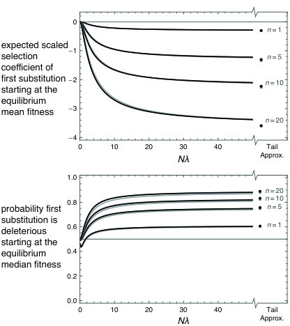
Figure 4 shows us that the evolutionary dynamics under FGM fall in one of two regimes, depending on the value of . When is very close to zero, the expected scaled selection coefficient of the first substitution is also close to zero (or indeed, sometimes very slightly positive). Similarly, in this regime, the fraction of substitutions that are deleterious is approximately one-half. Thus, if mutations have extremely small effects, the naive intuitions discussed in the Introduction are basically accurate.
However, when is greater than approximately 2, the situation is quite different: all of the qualitative results we derived for the HOC model also hold in this regime. In particular, the expected selection coefficient starting from the equilibrium mean fitness is negative; and the majority of substitutions starting from the equilibrium median fitness are deleterious (Figure 4). Furthermore, in this regime increasing the dimensionality of phenotype space decreases the expected scaled selection coefficient of the first substitution and increases the proportion deleterious first substitutions (Figure 4). This constitutes a “cost of complexity” (Orr, 2000) in that increasing the dimensionality of the phenotypic space makes the dynamics less favorable for an adapting population.
To better understand this large regime, it is helpful to note that both of our statistics of interest become less sensitive to as becomes large. In this regime, most mutations are deleterious and strongly selected against, which suggests that mutations destined for fixation will tend to come from the right tail of the mutational fitness distribution. Indeed, as becomes large, one can show that the mutational distribution converges to a tail approximation previously introduced by Martin and Lenormand (2008) (see Supporting Information S4.2). This tail approximation also suggests a method for deriving analytical results in the large regime. In particular, Martin and Lenormand (2008) derive a number of results using this tail approximation in conjunction with an approximation for the probability of fixation that allows only for advantageous fixations. By modifying their method to allow for the possibility of deleterious fixations, we obtain the following simple expression for the proportion of substitutions that will be advantageous, starting from the equilibrium median fitness (Supporting Information S4.3):
| (5) |
This expression clearly indicates that, in the large regime, the proportion of deleterious substitutions from the equilibrium median fitness exceeds and is an increasing function of the phenotypic dimensionality, . Applying similar methods to the expected scaled selection coefficient of the first substitution from the equilibrium mean fitness indicates that for large this quantity is 1) always negative and 2) solely a function of (Supporting Information S4.3).
Discussion
We have demonstrated that evolution can be dominated by deleterious substitutions in the short term even when adaptation will eventually occur over the long term. Critically, this initial decrease in fitness is not due to alleles that potentiate or otherwise promote the subsequent increase in fitness (Cowperthwaite et al., 2006), as would occur if these populations were crossing fitness valleys (Wright, 1932; Kimura, 1985; van Nimwegen and Crutchfield, 2000; Weinreich and Chao, 2005; Weissman et al., 2009). Rather, this decrease in fitness is due to unconditionally deleterious substitutions that have absolutely no effect other than to decrease the fitness of the population. Our results imply that studies of adaptation that ignore deleterious substitutions must give qualitatively incorrect predictions, at least in some regimes.
More precisely, we have considered a population evolving under a Moran process in the limit of weak mutation, where the fitnesses of new mutations are drawn independently from some fixed distribution (Kingman, 1977; Kingman, 1978, i.e., the house of cards model). Our results hold for arbitrarily large populations, and hence arbitrarily strong selection, under only the condition that a long-term equilibrium distribution exists with finite mean. This condition is always satisfied under the biologically plausible assumption that the probability that the next substitution be advantageous approaches zero as the fitness of a population increases to infinity.
Our two main results guarantee a region of initial fitnesses, below the equilibrium mean fitness, where the expected selection coefficient of the first substitution is negative; and a region of initial fitnesses, below the equilibrium median fitness, where the first substitution will be deleterious a majority of the time. In addition, we have shown qualitatively similar behavior under Fisher’s Geometric Model, where a “cost of complexity” (Orr, 2000; Martin and Lenormand, 2006) also arises, so that the magnitude of these effects becomes larger as the dimensionality of the phenotypic space increases (Fisher, 1930, c.f.).
Our results are surprising, and so it is important to develop some intuitions for why they hold. At the most basic level, our results are possible because the process of adaptation itself tends to increase fitness until the vast majority of possible mutations are deleterious (Hartl and Taubes, 1998; Silander et al., 2007). Indeed, this majority is eventually so vast that, at some sufficiently high fitness, deleterious mutations become responsible for the bulk of substitutions.
At a slightly more detailed level, the question is one of time scales: natural selection is so efficient that in the long term a population will spend most of its time at extremely rare, high-fitness alleles. However, the waiting time for such alleles to enter the population by mutation is extremely long, so that many populations will experience a deleterious substitution before even having the opportunity to fix an allele with high fitness. Thus, fitness may tend to decrease in the short term even though it will on average increase in the long term.
Finally, at a more mathematical level, our results follow from a deeper theorem that states that, no matter what the initial fitness, every quantile of the distribution of fitnesses after one substitution is less than the corresponding quantile of the equilibrium fitness distribution. We have used this deeper result to derive our two main results, but it has other consequences that we have not yet investigated in detail. For instance, consider a population that has experienced a recent change in environment or in population size, such that its current fitness is much higher than the equilibrium distribution. In this case, our result implies that the distribution of fitnesses after one substitution occurs will be to the left of the equilibrium distribution. Thus, fitness does not decrease to the new equilibrium by many small steps, but rather takes one large downhill jump.
The relationship between the equilibrium fitness distribution and the distribution of fitnesses after one substitution has an intuitive basis. In essence, high-fitness genotypes are occupied at high frequency in equilibrium for two distinct reasons:
- 1.
A population is more likely to become fixed for a high-fitness allele because the probability of fixation is greater for high-fitness mutations.
- 2.
Once fixed at a high-fitness allele, the time until the next fixation tends to be long, because of selection against deleterious substitutions.
While both of these factors push the equilibrium distribution towards very high fitnesses, only the first factor influences the distribution of fitnesses after one substitution. As a result, the distribution of fitnesses at equilibrium is always stochastically greater than the distribution of fitnesses after one substitution.
This distinction between the two factors above, and their different effects on evolution, is often neglected in the literature. In particular, the weak-mutation literature is primarily composed of two types of Markov models. In the first type of model, time is measured in units that are independent of when substitution events occur – so that time continues to elapse during the periods between subsequent substitution events in the population (Iwasa, 1988; Sella and Hirsh, 2005; Berg et al., 2004; Kryazhimskiy et al., 2009; McCandlish, 2013, see e.g.). In the second type of model, time is always discrete, and each unit of time corresponds to a single substitution event, no matter how long a population actually spends waiting in between substitution events (Gillespie, 1983; Gillespie, 1984; Hartl and Taubes, 1998; Orr, 2002; Weinreich et al., 2006; Draghi and Plotkin, 2013, e.g. ). Mathematically, a model of the first type is called the “full chain”; the corresponding model of the second type is called the “embedded chain”. Both of these Markov processes are important theoretical objects. However, while both of the above-mentioned factors influence the behavior of the full chain, only the first factor influences the behavior of the corresponding embedded chain. This means that the full chain and the embedded chain can have very different properties.
For instance, at equilibrium, evolution under the house of cards model is characterized by periods of rapid substitutions among relatively low-fitness alleles interspersed with long periods of stasis at high-fitness alleles (Iwasa, 1993). As a result, the equilibrium distribution of the full chain is concentrated at higher fitnesses than the equilibrium distribution of the embedded chain, since the embedded chain neglects the extra amount of time a population typically spends fixed at high-fitness alleles (more precisely, the probability density function of the equilibrium distribution for the embedded chain is proportional to , where the substitution rate is a decreasing function of ). Which type of these two equilibrium distributions is relevant for a particular purpose depends on whether one observes a population at a random time (as is most often the case for empirical data), in which case the full chain is appropriate; or whether one observes a population at a random substitution, in which case the embedded chain is appropriate.
Our results also have several important implications for the common practice of ignoring deleterious substitutions when studying adaptation. First, by demonstrating that adaptation can occur even when unconditionally deleterious substitutions dominate short-term evolution, we have shown that any satisfactory, general theory of adaptation must allow for the possibility of deleterious substitutions.
Second, our results characterize the conditions under which deleterious substitutions initially dominate the the adaptive process, i.e. when a majority of substitutions are deleterious or when fitness decreases in expectation. The range of parameters where deleterious substitutions play a non-negligible role is likely to be much larger.
Third, we emphasize that the frequency of deleterious substitutions changes as a population evolves. This frequency is therefore a property of the evolutionary dynamics rather than a parameter that can be assigned at the outset.
Finally, the problem of neglecting deleterious substitutions is particularly acute for studies that depend on “extreme value theory”, or “tail approximations,” because the mathematical methods underlying such studies assume the current fitness is already in the extreme right tail of the mutational fitness distribution. This is precisely the regime where we expect deleterious substitutions to be most important and therefore precisely the regime where they should not be neglected. One way forward for these studies is to incorporate approximations that allow deleterious substitutions to occur, as we did here in our analysis of Fisher’s Geometric Model.
An important limitation of our current analysis is that it has been conducted in the limit of weak mutation. It thus remains an open question how broadly these phenomena occur in other population-genetic regimes. However, a recent study of cancer progression by McFarland et al. (2013) suggests that similar dynamics, featuring a predominance of deleterious substitutions despite long-term adaptation, may occur even in populations with substantial polymorphism.
Acknowledgements
We thank Ricky Der and Mitchell Johnson for fruitful discussions and Warren Ewens for comments on the manuscript. J.B.P. acknowledges funding from the Burroughs Wellcome Fund, the David and Lucile Packard Foundation, the James S. McDonnell Foundation, the Alfred P. Sloan Foundation, the U.S. Department of the Interior (D12AP00025), and the Foundational Questions in Evolutionary Biology Fund (RFP-12-16). J.B.P., C.L.E. and D.M.M. acknowledge funding from the U.S. Army Research Office (W911NF-12-1-0552).
Literature Cited
- Berg et al. (2004) Berg, J., S. Willmann, and M. Lassig, 2004. Adaptive evolution of transcription factor binding sites. BMC Evol. Biol. 4:42. URL http://www.ncbi.nlm.nih.gov/pubmed/15511291.
- Chen and Rubin (1986) Chen, J. and H. Rubin, 1986. Bounds for the difference between median and mean of gamma and poisson distributions. Statistics & Probability Letters 4:281–283.
- Cowperthwaite et al. (2006) Cowperthwaite, M. C., J. Bull, and L. A. Meyers, 2006. From bad to good: Fitness reversals and the ascent of deleterious mutations. PLoS Comput. Biol. 2:e141.
- Crow and Kimura (1970) Crow, J. F. and M. Kimura, 1970. An Introduction To Population Genetics Theory. Blackburn Press, Caldwell, New Jersey.
- Draghi and Plotkin (2013) Draghi, J. A. and J. B. Plotkin, 2013. Selection biases the prevalence and type of epistasis along adaptive trajectories. Evolution URL http://dx.doi.org/10.1111/evo.12192.
- Fisher (1930) Fisher, R. A., 1930. The Genetical Theory of Natural Selection. Clarendon Press.
- Flyvbjerg and Lautrup (1992) Flyvbjerg, H. and B. Lautrup, 1992. Evolution in a rugged fitness landscape. Physical Review A 46:6714.
- Gillespie (1983) Gillespie, J. H., 1983. A simple stochastic gene substitution model. Theor. Popul. Biol. 23:202 – 215. URL http://www.sciencedirect.com/science/article/pii/004058098390%014X.
- Gillespie (1984) ———, 1984. Molecular evolution over the mutational landscapes. Evolution 38:1116 – 1129. URL http://www.jstor.org/stable/2408444.
- Gillespie (1994) ———, 1994. Substitution processes in molecular evolution. III. Deleterious alleles. Genetics 138:943 – 952. URL http://www.genetics.org/content/138/3/943.abstract.
- Haldane (1927) Haldane, J. B. S., 1927. A mathematical theory of natural and artificial selection, part V: Selection and mutation. Mathematical Proceedings of the Cambridge Philosophical Society 23:838 – 844. URL http://dx.doi.org/10.1017/S0305004100015644.
- Halligan and Keightley (2009) Halligan, D. L. and P. D. Keightley, 2009. Spontaneous mutation accumulation studies in evolutionary genetics. Annual Review of Ecology, Evolution, and Systematics 40:151–172.
- Hartl and Taubes (1998) Hartl, D. and C. Taubes, 1998. Towards a theory of evolutionary adaptation. Genetica 102-103:525 – 533. URL http://dx.doi.org/10.1023/A:1017071901530. 10.1023/A:1017071901530.
- Hartl and Taubes (1996) Hartl, D. L. and C. H. Taubes, 1996. Compensatory nearly neutral mutations: selection without adaptation. J. Theor. Biol. 182:303–309. URL http://dx.doi.org/10.1006/jtbi.1996.0168.
- Houle et al. (2011) Houle, D., C. Plabon, G. P. Wagner, and T. F. Hansen, 2011. Measurement and meaning in biology. Q. Rev. Biol. 86:3–34.
- Iwasa (1988) Iwasa, Y., 1988. Free fitness that always increases in evolution. J. Theor. Biol. 135:265 – 281. URL http://www.sciencedirect.com/science/article/pii/S00225193888%02431.
- Iwasa (1993) ———, 1993. Overdispersed molecular evolution in constant environments. J. Theor. Biol. 164:373 – 393. URL http://www.sciencedirect.com/science/article/pii/S00225193837%11616.
- Jain and Krug (2007) Jain, K. and J. Krug, 2007. Deterministic and stochastic regimes of asexual evolution on rugged fitness landscapes. Genetics 175:1275 – 1288.
- Jain and Seetharaman (2011) Jain, K. and S. Seetharaman, 2011. Multiple adaptive substitutions during evolution in novel environments. Genetics 189:1029 – 1043. URL http://www.genetics.org/content/189/3/1029.abstract.
- Joyce et al. (2008) Joyce, P., D. R. Rokyta, C. J. Beisel, and H. A. Orr, 2008. A general extreme value theory model for the adaptation of dna sequences under strong selection and weak mutation. Genetics 180:1627–1643. URL http://dx.doi.org/10.1534/genetics.108.088716.
- Kauffman and Levin (1987) Kauffman, S. and S. Levin, 1987. Towards a general theory of adaptive walks on rugged landscapes. J. Theor. Biol. 128:11 – 45.
- Kimura (1984) Kimura, M., 1984. The neutral theory of molecular evolution. Cambridge University Press.
- Kimura (1985) ———, 1985. The role of compensatory neutral mutations in molecular evolution. J. Genet. 64:7 – 19.
- Kingman (1977) Kingman, J., 1977. On the properties of bilinear models for the balance between genetic mutation and selection. in Mathematical Proceedings of the Cambridge Philosophical Society, vol. 81, Pp. 443–453. Cambridge Univ Press.
- Kingman (1978) ———, 1978. A simple model for the balance between selection and mutation. Journal of Applied Probability Pp. 1–12.
- Kryazhimskiy et al. (2009) Kryazhimskiy, S., G. Tkaçik, and J. B. Plotkin, 2009. The dynamics of adaptation on correlated fitness landscapes. Proc. Natl. Acad. Sci. U. S. A. 106:18638 – 18643. URL http://www.pnas.org/content/106/44/18638.abstract.
- Lourenço et al. (2011) Lourenço, J., N. Galtier, and S. Glémin, 2011. Complexity, pleiotropy, and the fitness effect of mutations. Evolution 65:1559–1571. URL http://dx.doi.org/10.1111/j.1558-5646.2011.01237.x.
- Lynch (2007) Lynch, M., 2007. The origins of genome architecture. Sinauer Associates Inc.
- Martin et al. (2007) Martin, G., S. F. Elena, and T. Lenormand, 2007. Distributions of epistasis in microbes fit predictions from a fitness landscape model. Nat. Genet. 39:555–560. URL http://dx.doi.org/10.1038/ng1998.
- Martin and Lenormand (2006) Martin, G. and T. Lenormand, 2006. A general multivariate extension of fisher’s geometrical model and the distribution of mutation fitness effects across species. Evolution 60:893–907.
- Martin and Lenormand (2008) ———, 2008. The distribution of beneficial and fixed mutation fitness effects close to an optimum. Genetics 179:907–916. URL http://dx.doi.org/10.1534/genetics.108.087122.
- McCandlish (2011) McCandlish, D. M., 2011. Visualizing fitness landscapes. Evolution 65:1544 – 1558. URL http://dx.doi.org/10.1111/j.1558-5646.2011.01236.x.
- McCandlish (2013) ———, 2013. On the findability of genotypes. Evolution URL http://dx.doi.org/10.1111/evo.12128.
- McCandlish et al. (In prep.) McCandlish, D. M., C. L. Epstein, and J. B. Plotkin, In prep. Formal properties of the probability of fixation: Identities, inequalities and approximations .
- McFarland et al. (2013) McFarland, C. D., K. S. Korolev, G. V. Kryukov, S. R. Sunyaev, and L. A. Mirny, 2013. Impact of deleterious passenger mutations on cancer progression. Proceedings of the National Academy of Sciences 110:2910–2915.
- Moran (1959) Moran, P. A. P., 1959. The survival of a mutant gene under selection. Journal of the Australian Mathematical Society 1:121 – 126.
- Ohta and Tachida (1990) Ohta, T. and H. Tachida, 1990. Theoretical study of near neutrality. I. Heterozygosity and rate of mutant substitution. Genetics 126:219 – 229. URL http://www.genetics.org/content/126/1/219.abstract.
- Orr (1998) Orr, H. A., 1998. The population genetics of adaptation: The distribution of factors fixed during adaptive evolution. Evolution 52:935 – 949. URL http://www.jstor.org/stable/2411226.
- Orr (2000) ———, 2000. Adaptation and the cost of complexity. Evolution 54:13–20.
- Orr (2002) ———, 2002. The population genetics of adaptation: The adaptation of DNA sequences. Evolution 56:1317 – 1330.
- Orr (2005) ———, 2005. The genetic theory of adaptation: A brief history. Nat. Rev. Genet. 6:119 – 127.
- Park and Krug (2008) Park, S.-C. and J. Krug, 2008. Evolution in random fitness landscapes: the infinite sites model. Journal of Statistical Mechanics: Theory and Experiment 2008:P04014.
- Poon and Otto (2000) Poon, A. and S. P. Otto, 2000. Compensating for our load of mutations: Freezing the meltdown of small populations. Evolution 54:1467 – 1479. URL http://dx.doi.org/10.1111/j.0014-3820.2000.tb00693.x.
- Sella and Hirsh (2005) Sella, G. and A. E. Hirsh, 2005. The application of statistical physics to evolutionary biology. Proc. Natl. Acad. Sci. U. S. A. 102:9541 – 9546. URL http://www.pnas.org/content/102/27/9541.abstract.
- Silander et al. (2007) Silander, O. K., O. Tenaillon, and L. Chao, 2007. Understanding the evolutionary fate of finite populations: the dynamics of mutational effects. PLoS Biol. 5:e94.
- Tachida (1991) Tachida, H., 1991. A study on a nearly neutral mutation model in finite populations. Genetics 128:183–192.
- Tachida (1996) ———, 1996. Effects of the shape of distribution of mutant effect in nearly neutral mutation models. J. Genet. 75:33–48.
- Tenaillon et al. (2007) Tenaillon, O., O. K. Silander, J.-P. Uzan, and L. Chao, 2007. Quantifying organismal complexity using a population genetic approach. PLoS One 2:e217. URL http://dx.doi.org/10.1371/journal.pone.0000217.
- van Nimwegen and Crutchfield (2000) van Nimwegen, E. and J. P. Crutchfield, 2000. Metastable evolutionary dynamics: Crossing fitness barriers or escaping via neutral paths? Bull. Math. Biol. 62:799 – 848.
- Wagner (2010) Wagner, G. P., 2010. The measurement theory of fitness. Evolution 64:1358–1376. URL http://dx.doi.org/10.1111/j.1558-5646.2009.00909.x.
- Waxman and Peck (1998) Waxman, D. and J. R. Peck, 1998. Pleiotropy and the preservation of perfection. Science 279:1210–1213.
- Weinreich and Chao (2005) Weinreich, D. M. and L. Chao, 2005. Rapid evolutionary escape by large populations from local fitness peaks is likely in nature. Evolution 59:1175 – 1182.
- Weinreich et al. (2006) Weinreich, D. M., N. F. Delaney, M. A. DePristo, and D. L. Hartl, 2006. Darwinian evolution can follow only very few mutational paths to fitter proteins. Science 312:111 – 114.
- Weissman et al. (2009) Weissman, D. B., M. M. Desai, D. S. Fisher, and M. W. Feldman, 2009. The rate at which asexual populations cross fitness valleys. Theor. Popul. Biol. 75:286 – 300.
- Welch and Waxman (2003) Welch, J. J. and D. Waxman, 2003. Modularity and the cost of complexity. Evolution 57:1723–1734.
- Wright (1932) Wright, S., 1932. The roles of mutation, inbreeding, crossbreeding and selection in evolution. in Proceedings of the Sixth International Congress of Genetics, Pp. 356 – 366.
Appendix A Proof of the main result
In this appendix, we provide a characterization of the distribution of fitnesses after one substitution. In particular, we provide bounds on the mean and cumulative distribution function of this distribution in terms of the means and cumulative distribution functions of the mutational fitness distribution, , and the corresponding equilibrium distribution, . Additional results describing how changing the initial fitness of the population changes the distribution of fitnesses after one substitution can be found in Supporting Information S1.
More formally, the distribution of fitnesses after one substitution has a probability density function given by , where is the substitution rate from to the interval and is the substitution rate at . In order to understand the structure of this distribution, we first state a very general result concerning the expected value of any non-decreasing function, , of fitness with respect to the distribution of fitnesses after one substitution as compared with the expected value of for fitnesses drawn from and . Deferring the proof of the main result until the end of this Appendix, we then state several corollaries corresponding to statements made in the main text, where these corollaries are derived by making specific choices for the non-decreasing function .
Here is the general result:
Theorem 1.
Under the house of cards model with a continuous mutational distribution and with , for any arbitrary initial fitness and non-decreasing, real-valued function defined on the real line, we have
| (A1) |
whenever the corresponding integrals are finite. The above inequalities are strict if there exist two open intervals of non-zero length within the support of such that the value of is strictly greater for members of the first interval than it is for members of the second.
Our biological results then follow by picking particular non-decreasing functions .
Corollary 2 (Expected fitness after one substitution).
For any , continuous probability distribution , and any choice of initial fitness:
- 1.
The expected Malthusian fitness after one substitution is strictly less than the expected Malthusian fitness at equilibrium and strictly greater than the expected Malthusian fitness of new mutations, should these expectations be finite.
- 2.
The expected Wrightean fitness after one substitution is strictly less than the expected Wrightean fitness at equilibrium and strictly greater than the expected Wrightean fitness of new mutations, should these expectations be finite.
Proof.
The first statement follows directly from Theorem 1 by choosing . This function is strictly increasing and so the condition for the strictness of the inequalities is satisfied. The second statement follows directly from Theorem 1 by choosing (Malthusian fitness is simply Wrightean fitness); this function is also strictly increasing and so the inequalities are strict. ∎
An immediate consequence of this corollary is that for a population that starts at the equilibrium mean fitness, the first substitution is expected to decrease fitness and so the expected selection coefficient of the first substitution is negative. The fact that the expected selection coefficient of the first substitution is a continuous function of the initial fitness (see Supporting Information S1 for a proof) implies the existence of some critical initial fitness, strictly less than the equilibrium mean fitness, such that the expected selection coefficient of the first substitution is always negative for initial fitnesses greater than this initial fitness, as stated in the main text. See also Supporting Information S1 for a proof that the expected selection coefficient of the first substitution is finite whenever either of 1) the mean fitness of new mutations or 2) the mean fitness at equilibrium is finite.
Corollary 3 (Cumulative distribution function of fitness after one substitution).
For , any continuous probability distribution , any choice of initial fitness , and for all fitnesses such that the probability that a new mutant has fitness less than or equal to is strictly between and , the cumulative distribution function of the distribution of fitnesses after one mutation is strictly less than the cumulative distribution function of the mutational distribution and, if an equilibrium distribution exists, strictly greater than the cumulative distribution function of the distribution of fitnesses at equilibrium.
Proof.
Let be the function that takes the value on the interval and 0 otherwise. Then Theorem 1 gives us:
| (A2) |
where the inequalities are strict since implies that there exists an open interval where with and another open interval where with . However, since probability distributions must integrate to , we also have
| (A3) |
as required. ∎
This corollary then allows us to prove the following result:
Corollary 4 (Quantiles of fitness after one substitution).
, any continuous probability distribution , any choice of initial fitness , and any choice of , the -th quantile of the distribution of fitnesses after one substitution is strictly greater than the -th quantile of the distribution of fitnesses introduced by mutation and, if an equilibrium distribution exists, strictly less than the -th quantile of the equilibrium fitness distribution.
Proof.
This follows immediately from Corollary 3 by choosing to be the -th quantile of the distribution of fitnesses after one substitution. ∎
Results about when a majority of substitutions are deleterious then follow from choosing and asking when this quantile is less than the initial fitness. If the initial fitness is the equilibrium median fitness, then the median fitness after one substitution is less than the initial fitness, meaning that the probability that the first substitution is deleterious is greater than . The fact that the probability that the first substitution is deleterious is continuous in the initial fitness (see Supporting Information S1 for a proof) then implies the existence of the critical initial fitness referred to in the main text.
Corollary 4 can also provide insight into the dynamics of a population at equilibrium. In particular, note that if the probability that the next substitution is deleterious was for each quantile of the equilibrium distribution, then the probability that the next substitution would be deleterious for a population whose fitness was drawn at random from the equilibrium distribution would be . However, Corollary 4 implies that the probability that the next substitution is deleterious at a particular fitness is always strictly greater than the quantile of that fitness in the equilibrium distribution. Thus, the probability that the next substitution is deleterious for a population whose fitness is drawn from the equilibrium distribution must be strictly greater than .
It is worth noting that the above results can all be extended to the case where the house of cards distribution is discrete or contains point masses (i.e. where is an arbitrary probability measure instead of a probability density function and expectation is interpreted in terms of Lebesgue integration). However, the statement of the results in this more general setting becomes more complex due to the non-zero probability of substitutions that are precisely neutral. See also Supporting Information S1 for additional proofs relating the distribution of fitnesses after one substitution for a population currently fixed at fitness to the corresponding distribution for a population currently fixed at some other fitness and a characterization of the behavior of the distribution of fitnesses after one substitution in the limit where the initial fitness tends to either or .
We now provide the proof for Theorem 1.
Proof.
Consider a non-decreasing function , and let
| (A4) | ||||
| (A5) |
be finite. The first thing we want to know is the sign of
| (A6) |
where we have used the fact that is a probability density and therefore integrates to one. Since it thus suffices to determine the sign of
| (A7) |
Now, define to be any fitness such that for and for . Such a fitness surely exists since is non-decreasing and . We can then write
| (A8) |
where the first integral on the right hand side is non-positive and the second integral is non-negative. Now, McCandlish et al. (In prep.) have proved that for and we have
| (A9) |
and the inequality is reversed for . Thus, for any three fitnesses, , and we have
| (A10) |
Using this inequality together with Equation A8 yields:
| (A11) |
where we have also used the definition of , the fact that is probability distribution and hence integrates to , and the definition of . This demonstrates the second inequality in the statement of the theorem, .
To see that this inequality is strict if there exist two open intervals of non-zero length within the support of such that is strictly greater on one of these intervals than it is on the other, notice that in the derivation of the first line of Equation A11 the inequality for the probability of fixation given by Equation A10 is strict. Thus, the first line of Equation A11 can only be an equality if both and . However if there exist two open intervals within the support of such that is strictly greater on one of these intervals than it is on the other, then there exists at least one of 1) some open interval within the support of with such that for or 2) some open interval within the support of with such that for . Now, for , so that the existence of implies that . Similarly, for so that the existence of implies that . Thus in either case the inequality is strict.
To prove the other inequality in the statement of the theorem, we proceed in a similar manner. Let
| (A12) |
be finite.
Now, we want to know the sign of , which takes the same sign as
| (A13) |
Choose to be a fitness such that for and for . Then
| (A14) |
where we have used the fact that for and for . This proves the first inequality in the statement of the theorem.
The argument for the strictness of this inequality if there exist two open intervals within the support of such that is strictly greater on one of these intervals than it is on the other is similar to the argument used for the other inequality and hinges on the strictness of the inequalities for and for used to derive the second line in Equation A14 rather than on the strictness of the inequalities in Equation A10. ∎
Supporting Information
Appendix Supporting Information S1 Additional results on the distribution of fitnesses after one substitution
This section of the Supporting Information contains additional results to complement those derived in Appendix A. First, we derive several results related to how the distribution of fitnesses after one substitution changes as the initial fitness is varied. Next, we derive conditions for when the expected value of a non-decreasing function is finite with respect to the distribution of fitnesses after one substitution. Finally, we prove that the substitution rate (), expected selection coefficient of the first substitution (), and proportion of the time the first substitution is advantageous () all change continuously as a function of initial fitness ().
The following result shows that the distribution of fitnesses after one substitution for a population fixed for fitness is to the left of the distribution of fitnesses after one substitution for a population fixed at fitness . The method of proof is similar to the proof of Theorem 1 in Appendix A but uses a different inequality for the probability of fixation.
Proposition S1.
Under the house of cards model with a continuous mutational distribution and , for any arbitrary initial fitnesses and with and any non-decreasing, real-valued function defined on the real line, we have
| (S1) |
whenever the corresponding integrals exist. The above inequality is strict if there exist two open intervals of length greater than zero within the support of such that the value of is strictly greater for members of the first interval than it is for members of the second.
Proof.
Let
| (S2) | ||||
| (S3) |
Also, let be any fitness such that for and for . Such a fitness surely exists since is increasing and .
We are interested in the sign of
| (S4) |
First, we expand
| (S5) |
where the first term on the right-hand side is non-positive and the second term in non-negative. Now McCandlish et al. (In prep.) have shown that for , and
| (S6) |
and that the inequality is reversed for . Thus, for any four fitnesses , , and with :
| (S7) |
Combining this inequality with Equation S5 yields:
| (S8) |
This demonstrates the inequality in the statement of the proposition. The justification for the condition on the strictness of the inequality is similar to that given in the proof of Theorem 1 except that it relies on the strictness of the inequalities in Equation S7. ∎
This proposition can then be used to show that the expected fitness after one substitution is increasing as a function of the initial fitness, and that, indeed, every quantile of the distribution of fitnesses after one substitution (except for the 0-th and 1-st) is increasing as a function of initial fitness. The proofs of these statements are exactly analogous to the proofs for Corollaries 2, 3 and 4 given in Appendix A.
We also wish to characterize the limit of the distribution of fitnesses after one substitution as the initial fitness becomes extremely large or extremely small. For technical reasons, we will conduct this proof in somewhat more generality than the previous proofs in that will be an arbitrary probability measure and all associated integrals will be Lebesgue integrals. Note that in this more general context it is still the case that an equilibrium measure
| (S9) |
exists for the stochastic process defined by Equation 2 provided that the normalizing constant is finite. We can now state the result:
Proposition S2.
For , we have
- 1.
For all fitnesses
(S10) - 2.
If exists, for all fitnesses
(S11)
Proof.
For the first statement in the theorem, we begin by characterizing
| (S12) |
Now, and , so that applying the Lebesgue dominated convergence theorem to move the limit inside the integral gives us
| (S13) |
where for the second equality have used the fact that . Thus
| (S14) |
This completes the proof of the first portion of the proposition
To address the second statement in the proposition, where , first observe that
| (S15) |
where we have used the identity . Then
| (S16) |
provided that the integral in the last line is finite, which it is since and by assumption. The two last facts also allow us to apply the Lebesgue dominated convergence theorem to move the limit inside the integral, which together with the fact that yields
| (S17) |
Using this last result and equation S15, we then have
| (S18) |
as required. ∎
Because many of our results describe inequalities for the expected value of a non-decreasing function with respect to , , and the distribution of fitnesses after one substitution, it is helpful to characterize when these expectations exist. The following result shows that if this expectation is finite with respect to either or , then it is also finite with respect to the distribution of fitnesses after one substitution:
Proposition S3.
Under the house of cards model with a continuous mutational distribution , , and any non- decreasing, real-valued function defined on the real line, we have
- 1.
If is finite for any , then it is finite for all .
- 2.
If is finite, then is finite for all .
- 3.
If is finite, then is finite for all .
Proof.
If is constant on the interior of the support of , then we are done, since then all the above integrals take this constant values. If is not constant on the interior of the support of , without loss of generality we can assume that takes both positive and negative values on the interior of the support of since otherwise we can simply consider a function for some such that is in the interior of the support of , which alters the values of the above integrals by but does not affect whether the integrals are finite.
Let be a constant such that for and for . To demonstrate the first claim, note that because for all , it suffices to show that is finite given that is finite for some . Because we will demonstrate the finiteness of these integrals using the limit comparison test, we must make a separate argument for each limit of these improper integrals. We thus consider and separately.
Now, and so that
| (S19) |
and
| (S20) |
Thus, we have
| (S21) |
which shows that is finite. Similarly, we have
| (S22) |
which shows that is finite.
To show the second claim, note that because for all , it suffices to show that both and are finite. This result follows because and we are given that and are finite.
To show the third claim, it suffices to show that and are finite, since then is finite for all by the first claim. To show that these integrals are finite, we note that for (McCandlish et al., In prep.) so that
| (S23) |
and
| (S24) |
as required. ∎
Finally, for Appendix A, we also need proofs that and are continuous functions of . First we need to prove some simpler results. We begin by proving that the substitution rate is continuous with respect to initial fitness.
Proposition S4.
is continuous in .
Proof.
First note that exists for all because so that . We want to show that for any , there exists a such that if then . In fact, in this case we can choose . First, we note that is continuous and (McCandlish et al., In prep.), so that , and thus . We then have
| (S25) |
as required. ∎
Note that since , the above proof has in fact demonstrated that for all . Thus is not merely continuous, but is rather Lipschitz continuous with Lipschitz constant .
Next, we prove a technical lemma.
Lemma S5.
If or has a finite mean, then is a continuous function of .
Proof.
If has finite mean, then . For , choose . Noting again that , for we have
| (S26) |
as required.
Now, suppose has finite mean so that . We first note that:
| (S27) |
where we have used the facts that and . Thus, for all ,
| (S28) |
Now, for any given choice of and choice of , pick such that , which is possible since can be made arbitrarily small. Using the identities and , for we have
| (S29) |
as required. ∎
Together, these results allow us to address the continuity of .
Proposition S6.
If or has finite mean then is a continuous function of .
Proof.
Finally, we address the continuity of .
Proposition S7.
is continuous in .
Proof.
Because
| (S31) |
and is both continuous (Proposition S4) and strictly positive, it suffices to show that is continuous in .
Now, for , choose such that and . It is always possible to choose an appropriate to satisfy the second inequality because we have assumed that is a continuous probability distribution, i.e. it has no point masses. Thus the total probability in an open ball of radius around can be made arbitrarily small by choosing a sufficiently small .
Appendix Supporting Information S2 The Gaussian HOC
In the main text, we claim that for the Gaussian HOC,
| (S35) |
for all and , where . To demonstrate this equality, it is sufficient to show that when viewed as a function of (i.e. with and held constant), since two probability density functions that are proportional to each other must be equal. Noting that for the Gaussian HOC , and that more generally , and , we have
| (S36) |
as required.
Appendix Supporting Information S3 Analytical approximations for the House of Cards model
It is often useful to develop analytical approximations for quantities of evolutionary interest. Here we present a system for developing analytical approximations under the House of Cards model. This system has the surprising feature that the terms in the analytical approximations are very closely related to the mutational and equilibrium distributions of the underlying House of Cards model.
Our main strategy is to extend the standard approximation for the probability of fixation, , to accommodate deleterious fixations:
| (S37) |
(McCandlish et al., In prep.). This approximation has the interesting property that when used in place of the true probability of fixation to define the transition rates in Equation 1, the resulting Markov process has an equilibrium distribution identical to the equilibrium distribution obtained using the true probability of fixation (Equation 4).
Using this approximation, we can then analyze the dynamics as follows. For a population fixed for an allele with fitness , the rate of beneficial substitutions, , is
| (S38) |
while the rate of deleterious fixations is
| (S39) |
Similarly, the expected instantaneous rate of change in fitness due to beneficial fixations is
| (S40) |
while the expected instantaneous rate of change in fitness due to deleterious fixations is
| (S41) |
To put this another way, approximating the substitution rate and the expected change in fitness for a population fixed for fitness comes down to calculating the first few moments of truncated versions of and . For many common distributions, these moments are easy to compute or can be looked up in a table (Jawitz, 2004, e.g., Table 1 of).
With these few quantities in hand, we can calculate a variety of other quantities of interest. Of course, the total substitution rate is
| (S42) |
and the probability that the next substitution is advantageous is
| (S43) |
Similarly, the expected instantaneous rate of change in fitness is
| (S44) |
and the expected selection coefficient of the first substitution is
| (S45) |
One can also compute the expected selection coefficient of the first substitution conditional on it being advantageous, , or deleterious, .
In the case when is normal with mean and variance , is normal with mean and the same variance. Let us write the cumulative distribution function of and as and , respectively. Looking up the necessary moments (Jawitz, 2004) and simplifying leads to the following expressions:
| (S46) | ||||
| (S47) | ||||
| (S48) | ||||
| (S49) |
It is interesting to ask why the above expressions are so symmetric. This is in large part a consequence of the fact that for our approximation of , it is still the case that and thus the symmetry argument given in Supporting Information S2 for the distribution of fitnesses after one substitution still holds under the approximation. As a consequence, the approximation is exactly correct for and , where .
The above equations were used to plot the curves in Figure 3. Note that the approximation, while reasonably good, is always more extreme than the numerical results, in the sense that, e.g., the analytical result for is too high when is positive and too low when is negative. This is to be expected, since our approximation underestimates the contribution of nearly neutral fixations and therefore overestimates the average magnitude of the mutations that fix.
Appendix Supporting Information S4 Results for Fisher’s Geometric Model
Supporting Information S4.1 Scaling of the model
In the main text, we note that evolution under Fisher’s geometric model is particularly easy to understand when fitnesses are measured in scaled fitness because then, to a very good approximation, the dynamics depend only on the dimensionality and the compound parameter . To see why this is the case, recall that the fitness of a mutant introduced by mutation when the current fitness is is times a non-central chi-squared distributed random variable with degrees of freedom and non-centrality parameter . Thus, if is the current scaled fitness, the scaled fitness of a new mutant is times a non-central chi-squared random variable with degrees of freedom and non-centrality parameter . Thus, the mutational process, when viewed in terms of scaled fitness, depends only on and the product .
Furthermore, it is well-known that the evolutionary dynamics under weak mutation depends primarily on scaled fitness, and not on fitness and population size separately, so long as selection coefficients remain small. In particular, if we approximate the probability of fixation as
| (S50) |
then the instantaneous transition rate from scaled fitness to scaled fitness is given by:
| (S51) |
where is the probability density function describing the scaled fitnesses of new mutations for a population whose current scaled fitness is (Kryazhimskiy et al., 2009). Since this probability density function depends only on , the compound parameter and the current fitness , it is clear that the dynamics of evolution under FGM when viewed in terms of scaled fitnesses depend only on and provided that the absolute size of the selection coefficients is sufficiently small.
Finally, using the above approximation for the transition rate from scaled fitness to scaled fitness yields a simple form for the equilibrium distribution. In particular the equilibrium distribution in terms of scaled fitnesses is times a gamma distribution with shape and scale 1. Note that this equilibrium distribution is independent of and that its mean is simply .
Supporting Information S4.2 The large limit
Having shown that the dynamics of evolution under FGM, to a good approximation, depend only on and when measured in terms of scaled fitnesses, it is natural to ask what happens in various limiting cases of these two parameters. Here we will discuss the dynamics as becomes large. In particular, we will take an approach based on approximating the distribution of scaled fitnesses introduced by mutation, , under the assumption that terms of order are negligible.
In order to investigate the large limit, it is helpful to write out the PDF of explicitly. Recalling that , we have:
| (S52) |
where is a modified Bessel function of the first kind:
| (S53) |
Following Martin and Lenormand (2008) in using the method of Jaschke et al. (2004), we then note that
| (S54) | |||
| (S55) |
so that
| (S56) |
We can thus make the approximation
| (S57) |
for large . Note that this is identical to the tail approximation for close to 0 used by Martin and Lenormand (2008) when translated into scaled fitness and adapted to the case of an isotropic FGM as analyzed here. This equivalence makes sense if we consider what happens if we make large by increasing while keeping and fixed, since then approaches 0 just as in the approximation developed by Martin and Lenormand (2008).
Supporting Information S4.3 Analytical approximations in the large limit
Given the approximation to the evolutionary dynamics for large developed in the previous section (Supporting Information S4.2), one can develop analytical results for the probability that the next substitution is advantageous and the expected scaled selection coefficient of the next substitution by using a further approximation for the probability of fixation. In particular, we will approximate the term:
| (S58) |
in Equation S51 as
| (S59) |
This approximation is very similar to the approximation used in Supporting Information S3 in that its use results in the same equilibrium distribution as the Markov process given by Equation S51. Importantly, this approximation can similarly be viewed as a modification of the standard approximation used in the literature on the genetics of adaptation (where the rate of advantageous substitutions is proportional to the selection coefficient) to accommodate the possibility of deleterious substitutions.
To begin, let us recall that for and
| (S60) |
and
| (S61) |
¥ where is an upper incomplete gamma function.
Using the first of the above integrals (Equation S60), we then have that the rate of advantageous substitution is
| (S62) |
Using the second of the above integrals (Equation S61), we also have that the rate of deleterious substitution is
| (S63) |
where we have used the recurrence relation to derive the last line. Thus, we have
| (S64) |
Notice that the probability in the last line is not a function of . Thus, while the absolute substitution rate at any fixed decreases for large as increases (see the factor in Equations S62 and S63), the fraction of beneficial substitutions approaches a definite limit as .
Now, if we approximate the median fitness at equilibrium by the mean fitness at equilibrium, Equation S64 shows that the probability that the next substitution is advantageous at the equilibrium median fitness is simply
| (S65) |
as stated in the main text (as a formal matter, the simplification arises because the term becomes if ). Critically, this expression is always less than for .
The expected selection coefficient of the first substitution, conditional on it being advantageous, can also be found using Equation S60:
| (S66) |
¥ which is equivalent to the expression given by Martin and Lenormand (2008) when the expression given by Martin and Lenormand (2008) is translated into scaled fitness. At the equilibrium mean fitness, this gives us
| (S67) |
Similarly, the expected selection coefficient of the first substitution, conditional on it being deleterious, can be found using Equation S61 and the recursive formula for the incomplete gamma function:
| (S68) |
¥ At the equilibrium mean fitness, this expression simplifies further to
| (S69) |
We can now use these results to characterize the expected selection coefficient of the first substitution for a population whose initial fitness is equal to the equilibrium mean fitness. The expected selection coefficient is given by:
| (S70) |
¥ which is solely a function of . Recalling the well-known inequality for (see, e.g., Olver et al., 2010, Section 8.10), we have
| (S71) |
¥ for , so that our approximation of is always negative.
Literature Cited in Supporting Information
- (1) DLMF, 2013. NIST Digital Library of Mathematical Functions. http://dlmf.nist.gov/, Release 1.0.6 of 2013-05-06. URL http://dlmf.nist.gov/. Online companion to Olver et al. (2010).
- Jaschke et al. (2004) Jaschke, S., C. Klüppelberg, and A. Lindner, 2004. Asymptotic behavior of tails and quantiles of quadratic forms of gaussian vectors. Journal of Multivariate Analysis 88:252–273.
- Jawitz (2004) Jawitz, J. W., 2004. Moments of truncated continuous univariate distributions. Advances in Water Resources 27:269–281.
- Kryazhimskiy et al. (2009) Kryazhimskiy, S., G. Tkaçik, and J. B. Plotkin, 2009. The dynamics of adaptation on correlated fitness landscapes. Proc. Natl. Acad. Sci. U. S. A. 106:18638 – 18643. URL http://www.pnas.org/content/106/44/18638.abstract.
- Martin and Lenormand (2008) Martin, G. and T. Lenormand, 2008. The distribution of beneficial and fixed mutation fitness effects close to an optimum. Genetics 179:907–916. URL http://dx.doi.org/10.1534/genetics.108.087122.
- McCandlish et al. (In prep.) McCandlish, D. M., C. L. Epstein, and J. B. Plotkin, In prep. Formal properties of the probability of fixation: Identities, inequalities and approximations .
- Olver et al. (2010) Olver, F. W. J., D. W. Lozier, R. F. Boisvert, and C. W. Clark (eds.) 2010. NIST Handbook of Mathematical Functions. Cambridge University Press, New York, NY. Print companion to DLMF ().