跳到论文正文
W Papers独立论文阅读器 arXiv:1309.0898 论文正文 计算阅读时间 · 0%
引用这篇论文根据当前论文元数据生成,正式投稿前建议核对。


License: arXiv.org perpetual non-exclusive license
arXiv:1309.0898v1 [cs.IT] 04 Sep 2013

Two-Hop Interference Channels:
Impact of Linear SchemesThanks: I. Issa, S. L. Fong, and A. S. Avestimehr are with the School of Electrical and Computer Engineering, Cornell University, Ithaca, NY (email: ii47@cornell.edu, lf338@cornell.edu, and avestimehr@ece.cornell.edu).Thanks: Preliminary parts of this work were presented at the 2013 International Symposium on Information Theory (ISIT)[1].

Ibrahim Issa, Silas L. Fong, and A. Salman Avestimehr Affiliation: 
Abstract

We consider the two-hop interference channel (IC), which consists of two source-destination pairs communicating with each other via two relays. We analyze the degrees of freedom (DoF) of this network when the relays are restricted to perform linear schemes, and the channel gains are constant (i.e., slow fading). We show that, somewhat surprisingly, by using vector-linear strategies at the relays, it is possible to achieve 4/3 sum-DoF when the channel gains are real. The key achievability idea is to alternate relaying coefficients across time, to create different end-to-end interference structures (or topologies) at different times. Although each of these topologies has only 1 sum-DoF, we manage to achieve 4/3 by coding across them. Furthermore, we develop a novel outer bound that matches our achievability, hence characterizing the sum-DoF of two-hop interference channels with linear schemes. As for the case of complex channel gains, we characterize the sum-DoF with linear schemes to be 5/3. We also generalize the results to the multi-antenna setting, characterizing the sum-DoF with linear schemes to be 2​M−1/32M-1/3 (for complex channel gains), where MM is the number of antennas at each node.

I Introduction

Multi-hopping is typically viewed as an effective approach to extend the coverage range of wireless networks, by bridging the gap between the sources and destinations via relays. However, it has also the potential to significantly impact network capacity by enabling new interference management techniques. For example, from the degrees of freedom (DoF) perspective, authors in [2] considered a two-hop complex interference channel (IC) consisting of two sources, two relays, and two destinations, and they showed by introducing a new scheme called aligned-interference-neutralization that the sum-DoF of this network is 2 (i.e., twice the sum-DoF of a single-hop IC). More recently, authors in [3] have considered two-hop interference networks with KK sources, KK relays, and KK destinations (i.e., K×K×KK\times K\times K network), and they showed by developing a new scheme named aligned-network-diagonalization that relays have the potential to asymptotically cancel the interference between all source-destination pairs, hence the cut-set bound is achievable (i.e., sum-DoF=KK).

While the aforementioned results essentially demonstrate that significant DoF gains can be achieved by carefully designing the interference management strategies in multi-hop interference networks, they often require complicated relaying strategies. For instance, for the case of time-varying channels, relays need to code over many independent channel realizations (i.e. requiring large channel diversity), and for the case of constant channels, they need to employ non-linear schemes and utilize large rational dimensions in order to align and neutralize interference. In this paper, we take a complementary approach and ask how much of these DoF gains can be realized if we limit the operation of relays to simple linear strategies?

We first consider the two-hop interference channel with constant and real channel gains (i.e., slow fading and baseband), and assume that the relays are allowed to perform only linear operations. It is easy to see that if we consider scalar-linear schemes with fixed amplify-forward (AF) coefficients at the relays, then the end-to-end channel is equivalent to a single-hop IC that has only 1 sum-DoF. We show that, surprisingly, by only allowing the relay AF coefficients to be time-varying (allowing for vector-linear schemes), we can exceed 1 sum-DoF and achieve 4/3. The key idea is as follows. With appropriate choice of amplify-forward coefficients at the relays, it is possible to create three specific end-to-end interference structures (or topologies), namely Z, S, or X. In short, the Z topology corresponds to the case that the end-to-end interference from source 1 to destination 2 is nulled, the S topology corresponds to the case that end-to-end interference from source 2 to destination 1 is nulled, and the X topology corresponds to the case that no end-to-end interference nulling has occurred. Although each of these topologies has only 1 sum-DoF, we show that it is possible to achieve 4/3 sum-DoF by creating different end-to-end topologies at different times, and employing an innovative coding strategy across them.

We also develop a novel outer bound on the DoF of two-hop IC with arbitrary vector-linear strategies that matches our achievability, thus characterizing the sum-DoF of two-hop IC using linear schemes to be 4/3. The main idea for the converse is the following. Consider a vector-linear scheme, where relays operate over blocks of ℓ\ell transmit symbols. In each block, the effective end-to-end channel (i.e., between the sources and the destinations) can be viewed as a multi-antenna IC with ℓ\ell antennas at each node, where we have some control over the channel realization through the choice of matrices at the relays. We prove that, regardless of the choice of relaying matrices, there exists a time-invariant linear relationship between each effective direct link and the effective interference links, which means that the end-to-end multi-antenna IC is ill-conditioned. This gives rise to a tension between decreasing the ranks of interference links and increasing the ranks of direct links. By carefully examining this tension, we prove that the sum-DoF is upper bounded by 4/3.

Next, we consider the setting with multiple antennas, say MM antennas, at each node (i.e. MIMO two-hop IC). This setup has been considered in [4], in which the authors show that, using lattice schemes, a sum-DoF of 2​M−12M-1 is achievable. Also, it is known that for this channel 2​M2M sum-DoF is achievable (i.e., the cut-set bound), by simply neglecting the possible cooperation between the antennas and applying the result of [3] for K×K×KK\times K\times K interference networks. Again, we ask what can we achieve if relays are restricted to linear strategies?

In the setting with MM antennas at each node, we characterize the sum-DoF of linear schemes to be 2​M−2/32M-2/3. The main idea for the achievability scheme is as follows. As before, the choice of relaying matrices dictates the end-to-end topology. However, in this setup, many topologies can be created, which makes the task of designing the scheme more difficult. We propose a 3-phase scheme which codes across 3 topologies, which we call the MIMO-S, MIMO-Z, and MIMO-X topologies. In the MIMO-S topology, all the end-to-end interference from source 2 is neutralized at destination 1, and only one antenna from source 1 causes interference at destination 2. Similarly, for the MIMO-Z topology, only one antenna from source 2 causes interference at destination 1. In the MIMO-X topology, however, one antenna from each source is causing interference at the other destination. The relaying matrices that create the above topologies correspond to the solutions of specific Sylvester equations11 1 The Sylvester equation is a matrix equation of the form A​X+X​B=CAX+XB=C, where AA, BB, CC, and XX are square matrices, and the problem is to find XX (for a given AA, BB, and CC)., with the constraint that the solutions are invertible. The conditions for the existence of such solutions have been studied extensively in the literature (e.g., [5, 6]). Using these results, we show that the aforementioned three topologies can be created for almost all values of the channel gains. Finally, we show that by coding across these topologies we can achieve 2​M−2/32M-2/3 sum-DoF.

As for the converse, the key ingredient is proving a relationship between the end-to-end direct links and end-to-end interference links. In particular, we show that if any of the direct links has full rank, then at least one of the interference links must be non-zero. This relationship, coupled with two genie-aided bounds, yields our result.

We also generalize the results to the case of complex channel gains. In the single-antenna case, it was shown in [2] that 3/2 sum-DoF is achievable by using a linear scheme based on asymmetric complex signaling. Also, more recently in [7], a new scheme named PCoF-CIA (Precoded Compute and Forward with Channel Integer Alignment) has been proposed to achieve 3/2 sum-DoF. We can evidently apply our scheme (designed for the case of real channel gains) and follow the same nulling and coding procedure to achieve 4/34/3 sum-DoF. However, we propose a better approach. We allow coding over the in-phase and quadrature-phase components of the channel, and show that, from the DoF perspective, the network can be viewed as a two-hop IC with real channel gains and 22-antennas at each node (corresponding to in-phase and quadrature-phase components). Then, by applying our scheme for the 2-antenna setting, we can achieve 4−2/34-2/3 real DoF in the equivalent network, which equates to 4−2/32=5/3\frac{4-2/3}{2}=5/3 sum-DoF in the original two-hop IC with complex channel gains. This improves over all previously known results with linear schemes. We also prove the optimality of our scheme, hence characterize the linear sum-DoF of two-hop IC with complex channel gains to be indeed 5/35/3. The results are also extended to the MM-antenna setting with complex channel gains, characterizing the linear sum-DoF to be 2​M−1/32M-1/3.

Finally, we present a numerical analysis of our proposed schemes. Although the main focus of this paper is the characterization of degrees of freedom (i.e., capacity analysis at high signal-to-noise ratio (SNR) regime), the simplicity of our schemes also allows for the analytical computation of the achieved rates at any finite SNR. Therefore, we compare our linear scheme for the two-hop IC with several state-of-the-art schemes, and demonstrate the capacity gains at finite SNR.

Other Related Works. Other than the aforementioned works that focus on the degrees of freedom of two-hop interference channels, there have also been several works on the capacity analysis of such networks. For example, authors in [8] approximate the capacity of networks of the form ZZ and ZS, using the deterministic approach [9]. In [10] and [11], authors adopt an approach that applies rate-splitting at the sources based on the Han-Kobayashi scheme [12], and decode-and-forward at the relays to cooperatively deliver the messages. However, this approach essentially treats the two-hop IC as a cascade of two interference channels, and thus cannot achieve more than 1 sum-DoF.

The rest of this paper is organized as follows. In Section II, we define the model and state our three main results. In Section III, we prove our first result for the single-antenna two-hop IC with real channel gains. In Section IV, we consider the MIMO two-hop IC with real channel gains, and we extend the result to the case of complex channel gains in Section V. Finally, in Section VI, we discuss our numerical results.

II Network Model & Statement of Main Results

The two-hop IC, illustrated in Figure 1, consists of two sources, two relays and two destinations. The two sources are indexed by s1s_{1} and s2s_{2}, the two relays are indexed by uu and vv and the two destinations are indexed by d1d_{1} and d2d_{2}. Each node is equipped with a single antenna22 2 The case for multi-antenna nodes will be discussed in Section IV.. The channel gains of the first hop are denoted by

𝐇𝟏=[hs1​uhs2​uhs1​vhs2​v]∈ℝ2×2,\mathbf{H_{1}}=\left[\begin{array}[]{cc}h_{s_{1}u}&h_{s_{2}u}\\ h_{s_{1}v}&h_{s_{2}v}\end{array}\right]\in\mathbb{R}^{2\times 2},

and the channel gains of the second hop are denoted by

𝐇𝟐=[hu​d1hv​d1hu​d2hv​d2]∈ℝ2×2.\mathbf{H_{2}}=\left[\begin{array}[]{cc}h_{ud_{1}}&h_{vd_{1}}\\ h_{ud_{2}}&h_{vd_{2}}\end{array}\right]\in\mathbb{R}^{2\times 2}.

We assume that the channel gains are real-valued and drawn from some continuous distribution, and fixed during the course of communication. All the nodes have the knowledge of 𝐇𝟏\mathbf{H_{1}} and 𝐇𝟐\mathbf{H_{2}}. For each i∈{1,2}i\in\{1,2\}, sis_{i} chooses a message Wi∈{1,2,…,2n​Ri}W_{i}\in\{1,2,\ldots,2^{nR_{i}}\} which is intended for did_{i} only. Each message WiW_{i} is uniformly distributed over {1,2,…,2n​Ri}\{1,2,\ldots,2^{nR_{i}}\}, and W1W_{1} and W2W_{2} are independent. The two sources transmit their messages to the destinations in nn time slots. For each i∈{1,2}i\in\{1,2\}, let Xi,k∈ℝX_{i,k}\in\mathbb{R} denote the symbol transmitted by source sis_{i} in the kthk^{\text{th}} time slot. Then, the symbols received in the same time slot by uu and vv, denoted by Yu,k∈ℝY_{u,k}\in\mathbb{R} and Yv,k∈ℝY_{v,k}\in\mathbb{R} respectively, satisfy

[Yu,kYv,k]=𝐇𝟏​[X1,kX2,k]+[Zu,kZv,k],\left[\begin{array}[]{c}Y_{u,k}\\ Y_{v,k}\end{array}\right]=\mathbf{H_{1}}\left[\begin{array}[]{c}X_{1,k}\\ X_{2,k}\end{array}\right]+\left[\begin{array}[]{c}Z_{u,k}\\ Z_{v,k}\end{array}\right], (1)

where Zu,k∼𝒩⁡(0,1)Z_{u,k}\sim\mathcal{N}(0,1) and Zv,k∼𝒩⁡(0,1)Z_{v,k}\sim\mathcal{N}(0,1). In addition, for each r∈{u,v}r\in\{u,v\}, let Xr,k∈ℝX_{r,k}\in\mathbb{R} denote the symbol transmitted by relay rr in the kthk^{\text{th}} time slot. Then, the symbols received in the same time slot by d1d_{1} and d2d_{2}, denoted by Y1,k∈ℝY_{1,k}\in\mathbb{R} and Y2,k∈ℝY_{2,k}\in\mathbb{R} respectively, satisfy

[Y1,kY2,k]=𝐇𝟐​[Xu,kXv,k]+[Z1,kZ2,k],\left[\begin{array}[]{c}Y_{1,k}\\ Y_{2,k}\end{array}\right]=\mathbf{H_{2}}\left[\begin{array}[]{c}X_{u,k}\\ X_{v,k}\end{array}\right]+\left[\begin{array}[]{c}Z_{1,k}\\ Z_{2,k}\end{array}\right], (2)

where Z1,k∼𝒩⁡(0,1)Z_{1,k}\sim\mathcal{N}(0,1) and Z2,k∼𝒩⁡(0,1)Z_{2,k}\sim\mathcal{N}(0,1). We assume that (X1n,X2n)(X_{1}^{n},X_{2}^{n}), ZunZ_{u}^{n}, ZvnZ_{v}^{n}, Z1nZ_{1}^{n}, and Z2nZ_{2}^{n} are independent, and we assume that {(Zu,k,Zv,k,Z1,k,Z2,k)}k=1n\{(Z_{u,k},Z_{v,k},Z_{1,k},Z_{2,k})\}_{k=1}^{n} are independent. After nn time slots, node did_{i} declares W^i\hat{W}_{i} to be the transmitted WiW_{i} based on YinY_{i}^{n} for each i∈{1,2}i\in\{1,2\}. For each i∈{1,2,u,v}i\in\{1,2,u,v\}, any codeword [xi,1​xi,2​…​xi,n]T[x_{i,1}\,x_{i,2}\,\ldots\,x_{i,n}]^{T} that is transmitted over the network should satisfy ‖xin‖2≤n​P||x_{i}^{n}||^{2}\leq nP, where PP represents the power constraint for all the nodes.

Refer to caption
Fig. 1: Two-hop IC.
Definition 1

An (n,R1,R2)(n,R_{1},R_{2})-code on the two-hop IC consists of the following:

  1. 1.

    A message set 𝒲i={1,2,…,2n​Ri}\mathcal{W}_{i}=\{1,2,\ldots,2^{nR_{i}}\} at sis_{i} for each i∈{1,2}i\in\{1,2\}.

  2. 2.

    An encoding function fi:𝒲i→ℝnf_{i}:\mathcal{W}_{i}\rightarrow\mathbb{R}^{n} at sis_{i} for each i∈{1,2}i\in\{1,2\} such that Xin=fi​(Wi)X_{i}^{n}=f_{i}(W_{i}). In addition, every codeword xinx_{i}^{n} must satisfy the power constraint ‖xin‖2≤n​P||x_{i}^{n}||^{2}\leq nP.

  3. 3.

    An encoding function fr,k:ℝk−1→ℝf_{r,k}:\mathbb{R}^{k-1}\rightarrow\mathbb{R} at each relay r∈{u,v}r\in\{u,v\} and each k∈{1,2,…,n}k\in\{1,2,\ldots,n\} such that Xr,k=fr,k​(Yrk−1)X_{r,k}=f_{r,k}(Y_{r}^{k-1}). In addition, every codeword xrnx_{r}^{n} must satisfy the power constraint ‖xrn‖2≤n​P||x_{r}^{n}||^{2}\leq nP.

  4. 4.

    A decoding function gi:ℝn→𝒲ig_{i}:\mathbb{R}^{n}\rightarrow\mathcal{W}_{i} at did_{i} for each i∈{1,2}i\in\{1,2\} such that W^i=gi​(Yin)\hat{W}_{i}=g_{i}(Y_{i}^{n}).

Without loss of generality, we assume

X1,k−=X2,k−=Zu,k−=Zv,k−=Yu,k−=Yv,k−=0X_{1,k^{-}}=X_{2,k^{-}}=Z_{u,k^{-}}=Z_{v,k^{-}}=Y_{u,k^{-}}=Y_{v,k^{-}}=0 (3)

for each k−≤0k^{-}\leq 0 in the rest of the paper.

Definition 2

For an (n,R1,R2)(n,R_{1},R_{2})-code, the average probability of decoding error of WiW_{i} is defined as Pe,in=ℙ𝕣{W^i≠Wi}P_{e,i}^{n}={\rm\mathbb{Pr}}\{\hat{W}_{i}\neq W_{i}\} for each i∈{1,2}i\in\{1,2\}.

Definition 3

Let ℓ\ell be a natural number and 𝒰\mathcal{U} be a finite set of real numbers. An (ℓ​n,R1,R2)(\ell n,R_{1},R_{2})-code on the two-hop IC is said to be ℓ\ell-linear on 𝒰\mathcal{U} if there exist {𝐀k∈𝒰ℓ×ℓ}k=1n\{\mathbf{A}_{k}\in\mathcal{U}^{\ell\times\ell}\}_{k=1}^{n} and {𝐁k∈𝒰ℓ×ℓ}k=1n\{\mathbf{B}_{k}\in\mathcal{U}^{\ell\times\ell}\}_{k=1}^{n} such that for each k∈{1,2,…,n}k\in\{1,2,\ldots,n\},

[Xu,ℓ⁡(k−1)+1Xu,ℓ⁡(k−1)+2…Xu,ℓ​k]T=𝐀k​[Yu,ℓ⁡(k−2)+1Yu,ℓ⁡(k−2)+2…Yu,ℓ⁡(k−1)]T\left[\begin{array}[]{cccc}X_{u,\ell(k-1)+1}&X_{u,\ell(k-1)+2}&\ldots&X_{u,\ell k}\end{array}\right]^{T}=\mathbf{A}_{k}\left[\begin{array}[]{cccc}Y_{u,\ell(k-2)+1}&Y_{u,\ell(k-2)+2}&\ldots&Y_{u,\ell(k-1)}\end{array}\right]^{T}

and

[Xv,ℓ⁡(k−1)+1Xv,ℓ⁡(k−1)+2…Xv,ℓ​k]T=𝐁k​[Yv,ℓ⁡(k−2)+1Yv,ℓ⁡(k−2)+2…Yv,ℓ⁡(k−1)]T.\left[\begin{array}[]{cccc}X_{v,\ell(k-1)+1}&X_{v,\ell(k-1)+2}&\ldots&X_{v,\ell k}\end{array}\right]^{T}=\mathbf{B}_{k}\left[\begin{array}[]{cccc}Y_{v,\ell(k-2)+1}&Y_{v,\ell(k-2)+2}&\ldots&Y_{v,\ell(k-1)}\end{array}\right]^{T}.

In other words, the relays are operating over blocks of length ℓ\ell, and the symbols in each transmitted block are linear combinations of the ℓ\ell symbols received in the previous block. We call ({𝐀k∈𝒰ℓ×ℓ}k=1n,{𝐁k∈𝒰ℓ×ℓ}k=1n)(\{\mathbf{A}_{k}\in\mathcal{U}^{\ell\times\ell}\}_{k=1}^{n},\{\mathbf{B}_{k}\in\mathcal{U}^{\ell\times\ell}\}_{k=1}^{n}) a relaying kernel of the code.

Definition 4

A rate pair (R1,R2)(R_{1},R_{2}) is ℓ\ell-linear achievable on 𝒰\mathcal{U} if there exists a sequence of (ℓ​n,R1,R2)(\ell n,R_{1},R_{2})-codes that are ℓ\ell-linear on 𝒰\mathcal{U} such that limn→∞Pe,iℓ​n=0\lim\limits_{n\rightarrow\infty}P_{e,i}^{\ell n}=0 for each i∈{1,2}i\in\{1,2\}.

Definition 5

The linear sum-DoF of the two-hop IC, denoted by 𝒟\mathcal{D}, is defined by

𝒟=supℓ,𝒰limP→∞sup{R1+R212​log2​P|(R1,R2) is ℓ-linear achievable on 𝒰}.\mathcal{D}=\sup_{\ell,\mathcal{U}}\lim_{P\rightarrow\infty}\!\sup\left\{\left.\frac{R_{1}+R_{2}}{\frac{1}{2}\log_{2}P}\>\right|(R_{1},R_{2})\text{ is $\ell$-linear achievable on }\mathcal{U}\right\}.

The first main result of this paper is the characterization of 𝒟\mathcal{D} as follows:

Theorem 1

The linear sum-DoF of the two-hop IC is 4/3 for almost all values of real channel gains. In particular, 𝒟=4/3\mathcal{D}=4/3 if the channel gains satisfy the following conditions:

  1. (c-1) All the channel gains are non-zero.

  2. (c-2) det​(𝐇i)≠0{\rm\text{det}}\left(\mathbf{H}_{i}\right)\neq 0 for each i∈{1,2}i\in\{1,2\}.

  3. (c-3) det​([hs2​u​hu​d1hs1​u​hu​d2hs2​v​hv​d1hs1​v​hv​d2])≠0{\rm\text{det}}\left(\left[\begin{array}[]{cc}h_{s_{2}u}h_{ud_{1}}&h_{s_{1}u}h_{ud_{2}}\\ h_{s_{2}v}h_{vd_{1}}&h_{s_{1}v}h_{vd_{2}}\end{array}\right]\right)\neq 0.

Remark 1

If we do not restrict the operations of the relays to be linear (i.e. we consider codes that satisfy Definition 1, but not necessarily Definition 3), then it is shown in [2] that 2 sum-DoF (i.e. the cut-set bound) is achievable using aligned interference neutralization. Theorem 1 shows that if we restrict the relays to simpler linear operations, then we can achieve 4/3 sum-DoF. Furthermore, unlike the channel conditions needed for [2] to achieve 2 sum-DoF , the above three conditions are insensitive to the rationality or irrationality of channel parameters.

In Section IV, we extend the result for the two-hop MIMO interference channel with real channel gains, where each node is equipped with MM antennas. We similarly define a linear code for this network in Section IV (cf. Definition 6), and then prove the second main result of our paper as follows.

Theorem 2

The linear sum-DoF of the two-hop MIMO IC with MM antennas at each node is 2​M−2/32M-2/3 for almost all values of real channel gains.

We finally extend Theorem 2 to complex channel gains and obtain the following corollary.

Corollary 1

The linear sum-DoF of the two-hop MIMO IC with MM antennas at each node is 2​M−1/32M-1/3 for almost all values of complex channel gains.

Remark 2

Note that the same achievability scheme used for the MIMO IC with real channel gains can be used for the one with complex channel gains, thus achieving 2​M−2/32M-2/3 sum-DoF for the complex case. However, we can get an additional gain by separating and coding over the in-phase and quadrature-phase components of the channel.

Remark 3

For the single-antenna two-hop IC with complex gains, authors in [2] and [7] propose schemes that achieve 3/2 sum-DoF without using rational dimensions, where the former relies on linear coding and the latter utilizes lattice coding and nulls the end-to-end interference by linear precoding/decoding over the finite field. Corollary 1 shows that we can actually exceed 3/2. In particular, it states that 5/3 sum-DoF is achievable using linear schemes.

Remark 4

In a recent result, authors in [4] show that for the two-hop MIMO IC with MM antennas at each node, 2​M−12M-1 sum-DoF is achievable using Precoded Compute and Forward (PCoF) with Channel Integer Alignment (CIA). Corollary 1 shows that linear schemes can also outperform PCoF with CIA in terms of sum-DoF.

Remark 5

Although the theorems above focus only on degrees of freedom, we can analytically compute the rates achieved by our proposed schemes at any SNR. We demonstrate the capacity gains at finite SNR as compared to state-of-the-art schemes in Section VI.

We will now proceed to prove Theorem 1, Theorem 2, and Corollary 1 in Sections III, IV, and V respectively.

III Two-Hop IC with Single-Antenna Nodes

In this section, we will prove Theorem 1. First, we describe a linear code that achieves 4/3 sum-DoF. Then, we will prove that 4/3 is an upper bound on the sum-DoF for any linear code.

III-A Achievability Proof of Theorem 1

We will show that ℓ\ell-linear schemes can achieve 4/3 sum-DoF if conditions (c-1)–(c-3) are satisfied. In particular, somewhat surprisingly, this can be done for ℓ=1\ell=1 only. In this case, the matrices chosen at the relays are just real scalars, however they can be time-varying.

The achievability scheme consists of three phases, during which each source sends two distinct symbols, and at the end of the three phases each receiver is able to reconstruct an interference-free (but noisy) version of its desired symbols.

For simplicity of notation, for ℓ=1\ell=1, set 𝐀k=αk\mathbf{A}_{k}=\alpha_{k} and 𝐁k=βk\mathbf{B}_{k}=\beta_{k}. Then the received signals at the destinations at each time kk can be written as

[Y1,kY2,k]=𝐇𝟐​[αk00βk]​𝐇𝟏​[X1,k−1X2,k−1]+[Z~1,kZ~2,k]=𝐆k​[X1,k−1X2,k−1]+[Z~1,kZ~2,k],\begin{split}\begin{bmatrix}Y_{1,k}\\ Y_{2,k}\end{bmatrix}&=\mathbf{H_{2}}\begin{bmatrix}\alpha_{k}&0\\ 0&\beta_{k}\end{bmatrix}\mathbf{H_{1}}\begin{bmatrix}X_{1,k-1}\\ X_{2,k-1}\end{bmatrix}+\begin{bmatrix}\tilde{Z}_{1,k}\\ \tilde{Z}_{2,k}\end{bmatrix}\\ &=\mathbf{G}_{k}\begin{bmatrix}X_{1,k-1}\\ X_{2,k-1}\end{bmatrix}+\begin{bmatrix}\tilde{Z}_{1,k}\\ \tilde{Z}_{2,k}\end{bmatrix},\end{split}

where

Z~i,k=hu​di​αk​Zu,k−1+hv​di​βk​Zv,k−1+Zi,k\tilde{Z}_{i,k}=h_{ud_{i}}\alpha_{k}Z_{u,k-1}+h_{vd_{i}}\beta_{k}Z_{v,k-1}+Z_{i,k}

is the effective noise at destination did_{i}, i∈{1,2}i\in\{1,2\}, and 𝐆k=𝐇𝟐​[αk00βk]​𝐇𝟏\mathbf{G}_{k}=\mathbf{H_{2}}\begin{bmatrix}\alpha_{k}&0\\ 0&\beta_{k}\end{bmatrix}\mathbf{H_{1}} is the equivalent end-to-end channel matrix given by

𝐆k=[hu​d1​hs1​u​αk+hv​d1​hs1​v​βkhu​d1​hs2​u​αk+hv​d1​hs2​v​βkhu​d2​hs1​u​αk+hv​d2​hs1​v​βkhu​d2​hs2​u​αk+hv​d2​hs2​v​βk].\mathbf{G}_{k}=\begin{bmatrix}h_{ud_{1}}h_{s_{1}u}\alpha_{k}+h_{vd_{1}}h_{s_{1}v}\beta_{k}&h_{ud_{1}}h_{s_{2}u}\alpha_{k}+h_{vd_{1}}h_{s_{2}v}\beta_{k}\\ h_{ud_{2}}h_{s_{1}u}\alpha_{k}+h_{vd_{2}}h_{s_{1}v}\beta_{k}&h_{ud_{2}}h_{s_{2}u}\alpha_{k}+h_{vd_{2}}h_{s_{2}v}\beta_{k}\end{bmatrix}.

For notational convenience, let 𝐆k=[g11,kg12,kg21,kg22,k]\mathbf{G}_{k}=\begin{bmatrix}g_{11,k}&g_{12,k}\\ g_{21,k}&g_{22,k}\end{bmatrix}. Then, the received signal at destination did_{i}, i∈{1,2}i\in\{1,2\}, at time kk is

Yi,k=gi​1,k​X1,k−1+gi​2,k​X2,k−1+Z~i,k, k∈{1,2,…,n}.Y_{i,k}=g_{i1,k}X_{1,k-1}+g_{i2,k}X_{2,k-1}+\tilde{Z}_{i,k},\text{\quad$k\in\{1,2,\dots,n\}$}. (4)

Note that the variance of Z~i,k\tilde{Z}_{i,k} depends only on channel gains and relay coefficients (chosen from 𝒰\mathcal{U}), therefore it does not scale with PP.

We will now describe the three phases of our linear achievability scheme in detail. Set

𝒰=c{0,1,−hu​d1hs2​u/hv​d1hs2​v,−hu​d2hs1​u/hv​d2hs1​v},\mathcal{U}=c\{0,1,-h_{ud_{1}}h_{s_{2}u}/h_{vd_{1}}h_{s_{2}v},-h_{ud_{2}}h_{s_{1}u}/h_{vd_{2}}h_{s_{1}v}\},

where the constant c∈ℝ+c\in\mathbb{R}^{+} is chosen to satisfy the power constraint PP at the relays. More specifically,

c=min⁡{1/(hs1​u2+hs2​u2+1),l​1/(hs1​v2+hs2​v2+1)},c=\min\left\{\sqrt{1/(h_{s_{1}u}^{2}\hskip-2.84526pt+h_{s_{2}u}^{2}\hskip-2.84526pt+1)},l\sqrt{1/(h_{s_{1}v}^{2}+h_{s_{2}v}^{2}+1)}\right\},

where l=min⁡{|hv​d1​hs2​v/hu​d1​hs2​u|,|hv​d2​hs1​v/hu​d2​hs1​u|}.l=\min\{{|h_{vd_{1}}h_{s_{2}v}/h_{ud_{1}}h_{s_{2}u}|,|h_{vd_{2}}h_{s_{1}v}/h_{ud_{2}}h_{s_{1}u}|}\}. Note that the denominators are non-zero by condition (c-1).

Phase 1. In this phase, s1s_{1} and s2s_{2} send two symbols a1a_{1} and b1b_{1} respectively (a12,b12≤P)(a_{1}^{2},b_{1}^{2}\leq P). We choose the relay coefficients such that the interference from s2s_{2} is canceled at d1d_{1}. More specifically, we set α1=c\alpha_{1}=c and β1=−chu​d1hs2​u/hv​d1hs2​v\beta_{1}=-ch_{ud_{1}}h_{s_{2}u}/h_{vd_{1}}h_{s_{2}v}. By inserting this choice of β1\beta_{1} and α1\alpha_{1} in (4), d1d_{1} and d2d_{2} will respectively receive

y1,1=g11,1​a1+z1,1, and ​y2,1=g21,1​a1+g22,1​b1⏟L1​(a1,b1)+z2,1,y_{1,1}=g_{11,1}a_{1}+z_{1,1},\text{ and }y_{2,1}=\underbrace{g_{21,1}a_{1}+g_{22,1}b_{1}}_{L_{1}(a_{1},b_{1})}+z_{2,1}, (5)

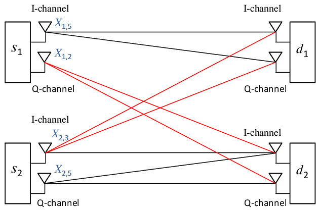
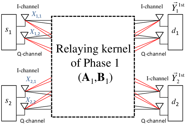
where g11,1≠0g_{11,1}\neq 0 and g22,1≠0g_{22,1}\neq 0 (due to conditions (c-1), (c-2), and (c-3)), and L1​(a1,b1)L_{1}(a_{1},b_{1}) indicates a linear equation in a1a_{1} and b1b_{1}. Thus, as shown in Figure 2(a), d1d_{1} and d2d_{2} now respectively have noisy versions of a1a_{1} and L1​(a1,b1)L_{1}(a_{1},b_{1}).

Refer to caption
(a) Phase 1
Refer to caption
(b) Phase 2
Refer to caption
(c) Phase 3
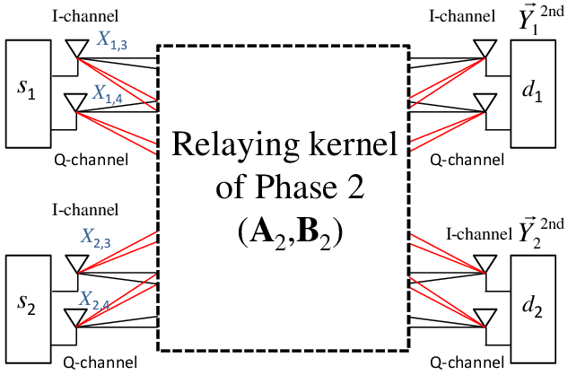
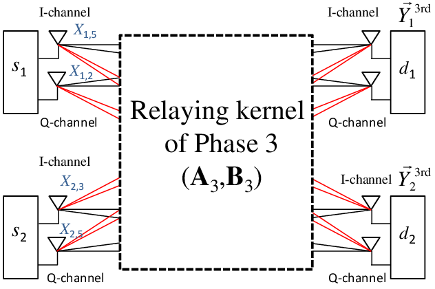
Fig. 2: Illustration of achievability scheme. At each phase, the transmit symbols by sources are shown on the left. The received signals at destinations are given on the right, where the noise is dropped and L⁡(x,y)L(x,y) denotes a linear combination of xx and yy.

Phase 2. In this phase, s1s_{1} and s2s_{2} send two new symbols a2a_{2} and b2b_{2} (a22,b22≤P)(a_{2}^{2},b_{2}^{2}\leq P). However, this time, we cancel the effect of s1s_{1} at d2d_{2}, by letting α2=c\alpha_{2}=c and β2=−chu​d2hs1​u/hv​d2hs1​v\beta_{2}=-ch_{ud_{2}}h_{s_{1}u}/h_{vd_{2}}h_{s_{1}v}. Then d1d_{1} and d2d_{2} will respectively receive

y1,2=g11,2​a2+g12,2​b2⏟L2​(a2,b2)+z1,2, and ​y2,1=g22,2​b2+z2,2,y_{1,2}=\underbrace{g_{11,2}a_{2}+g_{12,2}b_{2}}_{L_{2}(a_{2},b_{2})}+z_{1,2},\text{ and }y_{2,1}=g_{22,2}b_{2}+z_{2,2}, (6)

where g11,2≠0g_{11,2}\neq 0 and g22,2≠0g_{22,2}\neq 0 (due to conditions (c-1), (c-2), and (c-3)), and L2​(a2,b2)L_{2}(a_{2},b_{2}) indicates a linear equation in a2a_{2} and b2b_{2}. Thus, as shown in Figure 2(b), d1d_{1} and d2d_{2} now respectively have noisy versions of L2​(a2,b2)L_{2}(a_{2},b_{2}) and b2b_{2}.

Phase 3. Now notice that if, at phase 3, destination d1d_{1} receives a linear combination of a1a_{1} and b2b_{2} (L3​(a1,b2)L_{3}(a_{1},b_{2})), then it can solve for (a noisy version of) a2a_{2} given equations (5) and (6). Similarly, if d2d_{2} receives L4​(a1,b2)L_{4}(a_{1},b_{2}) then it can also solve for (a noisy version of) b1b_{1} given equations (5) and (6). Thus, as shown in Figure 2(c), in phase 3, s1s_{1} sends a1a_{1}, s2s_{2} sends b2b_{2}, and we choose α3=c\alpha_{3}=c and β3=0\beta_{3}=0, so that d1d_{1} and d2d_{2} receive

y1,3=g11,3​a1+g12,3​b2⏟L3​(a1,b2)+z1,3, and ​y2,3=g21,3​a1+g22,3​b2⏟L4​(a1,b2)+z2,3,y_{1,3}=\underbrace{g_{11,3}a_{1}+g_{12,3}b_{2}}_{L_{3}(a_{1},b_{2})}+z_{1,3},\text{ and }y_{2,3}=\underbrace{g_{21,3}a_{1}+g_{22,3}b_{2}}_{L_{4}(a_{1},b_{2})}+z_{2,3}, (7)

where g12,3≠0g_{12,3}\neq 0, and g21,3≠0g_{21,3}\neq 0 (due to condition (c-1)). Therefore, after the three phases, d1d_{1} can construct

y1a1=a1+z1,1/g11,1,y_{1}^{a_{1}}=a_{1}+z_{1,1}/g_{11,1}, (8)

and

y1a2=a2+1g11,2​z1,2−g12,2g11,2​g12,3​z1,3+g11,3​g12,2g11,1​g11,2​g12,3​z1,1.y_{1}^{a_{2}}=a_{2}+\frac{1}{g_{11,2}}z_{1,2}-\frac{g_{12,2}}{g_{11,2}g_{12,3}}z_{1,3}+\frac{g_{11,3}g_{12,2}}{g_{11,1}g_{11,2}g_{12,3}}z_{1,1}. (9)

from (y1,1,y1,2,y1,3)(y_{1,1},y_{1,2},y_{1,3}). Let σ12\sigma_{1}^{2} and σ22\sigma_{2}^{2} be the variances of the noise terms in equations (8) and (9). Note that they depend only on channel gains and relay coefficients. Hence, they are constants that do not scale with PP. Then, by using a proper outercode, we can achieve a rate of

R1\displaystyle R_{1} =16​(log⁡(1+Pσ12)+log⁡(1+Pσ22))\displaystyle=\frac{1}{6}\left(\log\left(1+\frac{P}{\sigma_{1}^{2}}\right)+\log\left(1+\frac{P}{\sigma_{2}^{2}}\right)\right) (10)
≥13​log⁡Pσ1​σ2.\displaystyle\geq\frac{1}{3}\log\frac{P}{\sigma_{1}\sigma_{2}}.

So d1d_{1} can achieve 2/32/3 DoF. Similarly, d2d_{2} can also achieve 2/32/3 DoF, hence achieving a total of 4/34/3 sum-DoF.

Remark 6

Note that the described scheme can also be viewed as a one-phase linear code with ℓ=3\ell=3, where s1s_{1} sends [a1a2a1]T\begin{bmatrix}a_{1}&a_{2}&a_{1}\end{bmatrix}^{T}, s2s_{2} sends [b1b2b2]T\begin{bmatrix}b_{1}&b_{2}&b_{2}\end{bmatrix}^{T}, and relays uu and vv set their amplifying matrices to be

𝐀1=[c000c000c]​ and ​𝐁1=[−chu​d1hs2​u/hv​d1hs2​v000−chu​d2hs1​u/hv​d2hs1​v0000]​ respectively.\mathbf{A}_{1}=\begin{bmatrix}c&0&0\\ 0&c&0\\ 0&0&c\end{bmatrix}\text{ and }\mathbf{B}_{1}=\begin{bmatrix}-ch_{ud_{1}}h_{s_{2}u}/h_{vd_{1}}h_{s_{2}v}&0&0\\ 0&-ch_{ud_{2}}h_{s_{1}u}/h_{vd_{2}}h_{s_{1}v}&0\\ 0&0&0\end{bmatrix}\text{ respectively.}

However, our initial description better illustrates the “spirit” of the scheme, in terms of understanding the choice of the amplifying factors at the relays and highlighting the opportunity of coding over different topologies. In fact, each individual topology shown in Figure 2 has a sum-DoF of 1, whilst we managed to achieve 4/3 sum-DoF by coding across them.

Remark 7

The coding strategy that is used in our scheme was first used for a binary fading IC, in which the channel links are either “on” or “off” [13, Appendix A]. A similar coding idea was also shown to be useful and provided DoF gains in the context of two-user IC with alternating connectivity [14].

III-B Converse Proof of Theorem 1

Assume (R1,R2)(R_{1},R_{2}) is ℓ\ell-achievable on 𝒰\mathcal{U} for some ℓ∈ℕ\ell\in\mathbb{N} and 𝒰⊂ℝ\mathcal{U}\subset\mathbb{R}. It then follows from Definition 4 that there exists a sequence of (ℓ​n,R1,R2)(\ell n,R_{1},R_{2})-codes that are ℓ\ell-linear on 𝒰\mathcal{U} such that

limn→∞Pe,iℓ​n=0\lim_{n\rightarrow\infty}P_{e,i}^{\ell n}=0 (11)

for each i∈{1,2}i\in\{1,2\}. We now fix this sequence of (ℓ​n,R1,R2)(\ell n,R_{1},R_{2})-codes and their corresponding relaying kernels ({𝐀k∈𝒰ℓ×ℓ}k=1n,{𝐁k∈𝒰ℓ×ℓ}k=1n)(\{\mathbf{A}_{k}\in\mathcal{U}^{\ell\times\ell}\}_{k=1}^{n},\{\mathbf{B}_{k}\in\mathcal{U}^{\ell\times\ell}\}_{k=1}^{n}). Let

ℓk={ℓ⁡(k−1)+1,ℓ⁡(k−1)+2,…,ℓ​k},\ell_{k}=\{\ell(k-1)+1,\ell(k-1)+2,\ldots,\ell k\},

where ℓk\ell_{k} represents the time slots of block kk. Then, at each block k∈{1,2,…,n}k\in\{1,2,\ldots,n\}, we have the following relationship between the received signals at the destinations and the transmit signals at the sources:

[Y1,ℓkY2,ℓk]\displaystyle\left[\begin{array}[]{c}Y_{1,\ell_{k}}\\ Y_{2,\ell_{k}}\end{array}\right] =(2)[hu​d1​Xu,ℓkhu​d2​Xu,ℓk]+[hv​d1​Xv,ℓkhv​d2​Xv,ℓk]+[Z1,ℓkZ2,ℓk]\displaystyle\stackrel{{\scriptstyle\eqref{secondChannelAddition}}}{{=}}\left[\begin{array}[]{c}h_{ud_{1}}X_{u,\ell_{k}}\\ h_{ud_{2}}X_{u,\ell_{k}}\end{array}\right]+\left[\begin{array}[]{c}h_{vd_{1}}X_{v,\ell_{k}}\\ h_{vd_{2}}X_{v,\ell_{k}}\end{array}\right]+\left[\begin{array}[]{c}Z_{1,\ell_{k}}\\ Z_{2,\ell_{k}}\end{array}\right]
=(a)[hu​d1​𝐀k​Yu,ℓk−1hu​d2​𝐀k​Yu,ℓk−1]+[hv​d1​𝐁k​Yv,ℓk−1hv​d2​𝐁k​Yv,ℓk−1]+[Z1,ℓkZ2,ℓk]\displaystyle\stackrel{{\scriptstyle\text{(a)}}}{{=}}\left[\begin{array}[]{c}h_{ud_{1}}\mathbf{A}_{k}Y_{u,\ell_{k-1}}\\ h_{ud_{2}}\mathbf{A}_{k}Y_{u,\ell_{k-1}}\end{array}\right]+\left[\begin{array}[]{c}h_{vd_{1}}\mathbf{B}_{k}Y_{v,\ell_{k-1}}\\ h_{vd_{2}}\mathbf{B}_{k}Y_{v,\ell_{k-1}}\end{array}\right]+\left[\begin{array}[]{c}Z_{1,\ell_{k}}\\ Z_{2,\ell_{k}}\end{array}\right]
=(b)[𝐆𝟏𝟏,k𝐆𝟏𝟐,k𝐆𝟐𝟏,k𝐆𝟐𝟐,k]​[X1,ℓk−1X2,ℓk−1]+[hu​d1​𝐀khv​d1​𝐁khu​d2​𝐀khv​d2​𝐁k]​[Zu,ℓk−1Zv,ℓk−1]+[Z1,ℓkZ2,ℓk],\displaystyle\stackrel{{\scriptstyle\text{(b)}}}{{=}}\left[\begin{array}[]{cc}\mathbf{G}_{\mathbf{11},k}&\mathbf{G}_{\mathbf{12},k}\\ \mathbf{G}_{\mathbf{21},k}&\mathbf{G}_{\mathbf{22},k}\end{array}\right]\left[\begin{array}[]{c}X_{1,\ell_{k-1}}\\ X_{2,\ell_{k-1}}\end{array}\right]+\left[\begin{array}[]{cc}h_{ud_{1}}\mathbf{A}_{k}&h_{vd_{1}}\mathbf{B}_{k}\\ h_{ud_{2}}\mathbf{A}_{k}&h_{vd_{2}}\mathbf{B}_{k}\end{array}\right]\left[\begin{array}[]{c}Z_{u,\ell_{k-1}}\\ Z_{v,\ell_{k-1}}\end{array}\right]+\left[\begin{array}[]{c}Z_{1,\ell_{k}}\\ Z_{2,\ell_{k}}\end{array}\right],

where

  1. (a)

    follows from Definition 3.

  2. (b)

    follows from substituting Yu,ℓk−1Y_{u,\ell_{k-1}} and Yv,ℓk−1Y_{v,\ell_{k-1}} by (1) and defining the end-to-end matrix from sjs_{j} to did_{i}, denoted by 𝐆𝐢𝐣,k\mathbf{G}_{\mathbf{ij},k}, for each k∈{1,2,…,n}k\in\{1,2,\ldots,n\} as follows:

    𝐆𝐢𝐣,k=hsj​u​hu​di​𝐀k+hsj​v​hv​di​𝐁k.\mathbf{G}_{\mathbf{ij},k}=h_{s_{j}u}h_{ud_{i}}\mathbf{A}_{k}+h_{s_{j}v}h_{vd_{i}}\mathbf{B}_{k}. (36)

In addition, for each i∈{1,2}i\in\{1,2\}, let

Pk=𝔼⁡[‖X1,ℓk‖2+‖X2,ℓk‖2]P_{k}={\rm\mathbb{E}}[||X_{1,\ell_{k}}||^{2}+||X_{2,\ell_{k}}||^{2}] (37)

be the average sum-power of block kk transmitted by the sources, which is averaged over the codebooks of the sources. We state the following key lemma which implies 𝒟≤4/3\mathcal{D}\leq 4/3.

Lemma 2

For any sequence of (ℓ​n,R1,R2)(\ell n,R_{1},R_{2})-codes and their corresponding 𝐆𝐢𝐣,k\mathbf{G}_{\mathbf{ij},k} as defined above, we have for sufficiently large nn

R1+R2≤τ1+12​ℓ​n​∑k=1n(rank⁡(𝐆𝟐𝟏,k)+rank⁡(𝐆𝟐𝟏,k))​log2⁡(1+Pk−1/ℓ),R_{1}+R_{2}\leq\tau_{1}+\frac{1}{2\ell n}\sum_{k=1}^{n}({\rm{rank}}(\mathbf{G}_{\mathbf{21},k})+{\rm{rank}}(\mathbf{G}_{\mathbf{21},k}))\log_{2}(1+P_{k-1}/\ell), Bound (i)
R1+R2≤τ2+12​ℓ​n∑k=1n(2ℓ−rank(𝐆𝟏𝟐,k))log2(1+Pk−1/ℓ])R_{1}+R_{2}\leq\tau_{2}+\frac{1}{2\ell n}\sum_{k=1}^{n}(2\ell-{\rm{rank}}(\mathbf{G}_{\mathbf{12},k}))\log_{2}(1+P_{k-1}/\ell]) Bound (ii)

and

R1+R2≤τ3+12​ℓ​n​∑k=1n(2​ℓ−rank⁡(𝐆𝟐𝟏,k))​log2⁡(1+Pk−1/ℓ),R_{1}+R_{2}\leq\tau_{3}+\frac{1}{2\ell n}\sum_{k=1}^{n}(2\ell-{\rm{rank}}(\mathbf{G}_{\mathbf{21},k}))\log_{2}(1+P_{k-1}/\ell), Bound (iii)

where Pk−1P_{k-1} is defined in (37), and τ1\tau_{1}, τ2\tau_{2} and τ3\tau_{3} are some constants that do not depend on nn and PP.

Before proving Lemma 2, we demonstrate how it implies 𝒟≤4/3\mathcal{D}\leq 4/3 and hence Theorem 1. Summing Bound (i), Bound (ii) and Bound (iii) in Lemma 2 and dividing 33 on both sides of the resultant inequality, we have for sufficiently large nn

R1+R2\displaystyle R_{1}+R_{2} ≤τ1+τ2+τ33+23​n​∑k=1nlog2⁡(1+Pk−1/ℓ)\displaystyle\leq\frac{\tau_{1}+\tau_{2}+\tau_{3}}{3}+\frac{2}{3n}\sum_{k=1}^{n}\log_{2}(1+P_{k-1}/\ell)
≤(3)τ1+τ2+τ33+23​n​∑k=1nlog2⁡(1+Pk/ℓ)\displaystyle\stackrel{{\scriptstyle\eqref{zeroConvention}}}{{\leq}}\frac{\tau_{1}+\tau_{2}+\tau_{3}}{3}+\frac{2}{3n}\sum_{k=1}^{n}\log_{2}(1+P_{k}/\ell)
≤(a)τ1+τ2+τ33+23​log2⁡(1+∑k=1nPkℓ​n)\displaystyle\stackrel{{\scriptstyle\text{(a)}}}{{\leq}}\frac{\tau_{1}+\tau_{2}+\tau_{3}}{3}+\frac{2}{3}\log_{2}\left(1+\frac{\sum_{k=1}^{n}P_{k}}{\ell n}\right)
≤(b)τ1+τ2+τ33+23​log2⁡(1+2​P),\displaystyle\stackrel{{\scriptstyle\text{(b)}}}{{\leq}}\frac{\tau_{1}+\tau_{2}+\tau_{3}}{3}+\frac{2}{3}\log_{2}(1+2P), (38)

where

  1. (a)

    follows from applying Jensen’s inequality to the concave function log2⁡(1+x)\log_{2}(1+x).

  2. (b)

    follows from Definition 1 that ‖Xiℓ​n‖2≤ℓ​n​P||X_{i}^{\ell n}||^{2}\leq\ell nP for each i∈{1,2}i\in\{1,2\}.

It then follows from (38) and Definition 5 that 𝒟≤4/3\mathcal{D}\leq 4/3. We now proceed to prove Lemma 2.

III-B1 Proof for Bound (i) in Lemma 2

Fix a sequence of (ℓ​n,R1,R2)(\ell n,R_{1},R_{2})-codes and their corresponding 𝐆𝐢𝐣,k\mathbf{G}_{\mathbf{ij},k}. Let

Y~1,ℓk=𝐆𝟏𝟏,k​X1,ℓk−1+𝐆𝟏𝟐,k​X2,ℓk−1+Z1,ℓk\tilde{Y}_{1,\ell_{k}}=\mathbf{G}_{\mathbf{11},k}X_{1,\ell_{k-1}}+\mathbf{G}_{\mathbf{12},k}X_{2,\ell_{k-1}}+Z_{1,\ell_{k}} (39)

and

Y~2,ℓk=𝐆𝟐𝟏,k​X1,ℓk−1+𝐆𝟐𝟐,k​X2,ℓk−1+Z2,ℓk\tilde{Y}_{2,\ell_{k}}=\mathbf{G}_{\mathbf{21},k}X_{1,\ell_{k-1}}+\mathbf{G}_{\mathbf{22},k}X_{2,\ell_{k-1}}+Z_{2,\ell_{k}} (40)

be less noisy versions of Y1,ℓkY_{1,\ell_{k}} and Y2,ℓkY_{2,\ell_{k}} respectively for each k∈{1,2,…,n}k\in\{1,2,\ldots,n\} (i.e., removing the impact of Zu,ℓk−1Z_{u,\ell_{k-1}} and Zv,ℓk−1Z_{v,\ell_{k-1}} in (III-B)). Since WiW_{i} is uniformly distributed over {1,2,…,2ℓ​n​Ri}\{1,2,\ldots,2^{\ell nR_{i}}\} for each i∈{1,2}i\in\{1,2\}, it follows that

ℓ​n​(R1+R2)\displaystyle\ell n(R_{1}+R_{2})
=H⁡(W1)+H⁡(W2)\displaystyle=H(W_{1})+H(W_{2})
=I⁡(W1,Y~1ℓ​n)+I⁡(W2,Y~2ℓ​n)+H⁡(W1|Y~1ℓ​n)+H⁡(W2|Y~2ℓ​n)\displaystyle=I(W_{1};\tilde{Y}_{1}^{\ell n})+I(W_{2};\tilde{Y}_{2}^{\ell n})+H(W_{1}|\tilde{Y}_{1}^{\ell n})+H(W_{2}|\tilde{Y}_{2}^{\ell n})
≤(a)I⁡(X1ℓ​n,Y~1ℓ​n)+I⁡(X2ℓ​n,Y~2ℓ​n)+H⁡(W1|Y~1ℓ​n)+H⁡(W2|Y~2ℓ​n)\displaystyle\stackrel{{\scriptstyle\text{(a)}}}{{\leq}}I(X_{1}^{\ell n};\tilde{Y}_{1}^{\ell n})+I(X_{2}^{\ell n};\tilde{Y}_{2}^{\ell n})+H(W_{1}|\tilde{Y}_{1}^{\ell n})+H(W_{2}|\tilde{Y}_{2}^{\ell n})
=(b)I⁡(X1ℓ​n,Y~1ℓ​n)+I⁡(X2ℓ​n,Y~2ℓ​n)+H⁡(W1|Y~1ℓ​n,Zuℓ​n,Zvℓ​n)+H⁡(W2|Y~2ℓ​n,Zuℓ​n,Zvℓ​n)\displaystyle\stackrel{{\scriptstyle\text{(b)}}}{{=}}I(X_{1}^{\ell n};\tilde{Y}_{1}^{\ell n})+I(X_{2}^{\ell n};\tilde{Y}_{2}^{\ell n})+H(W_{1}|\tilde{Y}_{1}^{\ell n},Z_{u}^{\ell n},Z_{v}^{\ell n})+H(W_{2}|\tilde{Y}_{2}^{\ell n},Z_{u}^{\ell n},Z_{v}^{\ell n})
≤(c)I⁡(X1ℓ​n,Y~1ℓ​n)+I⁡(X2ℓ​n,Y~2ℓ​n)+H⁡(W1|Y1ℓ​n)+H⁡(W2|Y2ℓ​n)\displaystyle\stackrel{{\scriptstyle\text{(c)}}}{{\leq}}I(X_{1}^{\ell n};\tilde{Y}_{1}^{\ell n})+I(X_{2}^{\ell n};\tilde{Y}_{2}^{\ell n})+H(W_{1}|Y_{1}^{\ell n})+H(W_{2}|Y_{2}^{\ell n})
≤(d)I⁡(X1ℓ​n,Y~1ℓ​n)+I⁡(X2ℓ​n,Y~2ℓ​n)+2+Pe,1ℓ​n​ℓ​n​R1+Pe,2ℓ​n​ℓ​n​R2\displaystyle\stackrel{{\scriptstyle\text{(d)}}}{{\leq}}I(X_{1}^{\ell n};\tilde{Y}_{1}^{\ell n})+I(X_{2}^{\ell n};\tilde{Y}_{2}^{\ell n})+2+P_{e,1}^{\ell n}\ell nR_{1}+P_{e,2}^{\ell n}\ell nR_{2} (41)

where

  1. (a)

    follows from Definition 1, (39) and (40) that Wi→Xiℓ​n→Y~iℓ​nW_{i}\rightarrow X_{i}^{\ell n}\rightarrow\tilde{Y}_{i}^{\ell n} forms a Markov Chain for each i∈{1,2}i\in\{1,2\}.

  2. (b)

    follows from the fact that (W1,W2,Y~1ℓ​n,Y~2ℓ​n)(W_{1},W_{2},\tilde{Y}_{1}^{\ell n},\tilde{Y}_{2}^{\ell n}) and (Zuℓ​n,Zvℓ​n)(Z_{u}^{\ell n},Z_{v}^{\ell n}) are independent.

  3. (c)

    follows from the fact that for each i∈{1,2}i\in\{1,2\}, Yiℓ​nY_{i}^{\ell n} is a function of (Y~iℓ​n,Zuℓ​n,Zvℓ​n)(\tilde{Y}_{i}^{\ell n},Z_{u}^{\ell n},Z_{v}^{\ell n}) (cf. (III-B), (39) and (40)).

  4. (d)

    follows from Fano’s inequality.

We now state the following lemma, proved in Appendix A, to upper bound I⁡(X1ℓ​n,Y~1ℓ​n)+I⁡(X2ℓ​n,Y~2ℓ​n)I(X_{1}^{\ell n};\tilde{Y}_{1}^{\ell n})+I(X_{2}^{\ell n};\tilde{Y}_{2}^{\ell n}) in (41).

Lemma 3

For any sequence of (ℓ​n,R1,R2)(\ell n,R_{1},R_{2})-codes with their corresponding 𝐆𝐢𝐣,k\mathbf{G}_{\mathbf{ij},k}, there exist four real numbers denoted by λ1\lambda_{1}, λ2\lambda_{2}, μ1\mu_{1} and μ2\mu_{2}. which are only functions of (𝐇𝟏,𝐇𝟐)(\mathbf{H_{1}},\mathbf{H_{2}}), such that

𝐆𝟏𝟏,k=λ1​𝐆𝟏𝟐,k+λ2​𝐆𝟐𝟏,k\mathbf{G}_{\mathbf{11},k}=\lambda_{1}\mathbf{G}_{\mathbf{12},k}+\lambda_{2}\mathbf{G}_{\mathbf{21},k} (42)

and

𝐆𝟐𝟐,k=μ1​𝐆𝟏𝟐,k+μ2​𝐆𝟐𝟏,k\mathbf{G}_{\mathbf{22},k}=\mu_{1}\mathbf{G}_{\mathbf{12},k}+\mu_{2}\mathbf{G}_{\mathbf{21},k} (43)

for all k∈{1,2,…,n}k\in\{1,2,\ldots,n\}.

The importance of Lemma 3 is that it captures the relationship between the direct links and the interference links. More specifically, it expresses the direct links as explicit functions of the interference links. This means that the corresponding MIMO channel, described by equation (III-B), is ill-conditioned. Using (42) and (43) in Lemma 3, we obtain from (39) and (40) that

Y~1,ℓk=(λ1​𝐆𝟏𝟐,k+λ2​𝐆𝟐𝟏,k)​X1,ℓk−1+𝐆𝟏𝟐,k​X2,ℓk−1+Z1,ℓk\tilde{Y}_{1,\ell_{k}}=(\lambda_{1}\mathbf{G}_{\mathbf{12},k}+\lambda_{2}\mathbf{G}_{\mathbf{21},k})X_{1,\ell_{k-1}}+\mathbf{G}_{\mathbf{12},k}X_{2,\ell_{k-1}}+Z_{1,\ell_{k}} (44)

and

Y~2,ℓk=𝐆𝟐𝟏,k​X1,ℓk−1+(μ1​𝐆𝟏𝟐,k+μ2​𝐆𝟐𝟏,k)​X2,ℓk−1+Z2,ℓk\tilde{Y}_{2,\ell_{k}}=\mathbf{G}_{\mathbf{21},k}X_{1,\ell_{k-1}}+(\mu_{1}\mathbf{G}_{\mathbf{12},k}+\mu_{2}\mathbf{G}_{\mathbf{21},k})X_{2,\ell_{k-1}}+Z_{2,\ell_{k}} (45)

for each k∈{1,2,…,n}k\in\{1,2,\ldots,n\}. Following (41), we consider

I⁡(X1ℓ​n,Y~1ℓ​n)+I⁡(X2ℓ​n,Y~2ℓ​n)\displaystyle I(X_{1}^{\ell n};\tilde{Y}_{1}^{\ell n})+I(X_{2}^{\ell n};\tilde{Y}_{2}^{\ell n})
=h⁡(Y~1ℓ​n)−h⁡(Y~2ℓ​n|X2ℓ​n)+h⁡(Y~2ℓ​n)−h⁡(Y~1ℓ​n|X1ℓ​n)\displaystyle=h(\tilde{Y}_{1}^{\ell n})-h(\tilde{Y}_{2}^{\ell n}|X_{2}^{\ell n})+h(\tilde{Y}_{2}^{\ell n})-h(\tilde{Y}_{1}^{\ell n}|X_{1}^{\ell n})
=(a)h⁡({(λ1​𝐆𝟏𝟐,k+λ2​𝐆𝟐𝟏,k)​X1,ℓk−1+𝐆𝟏𝟐,k​X2,ℓk−1+Z1,ℓk}k=1n)−h⁡({𝐆𝟐𝟏,k​X1,ℓk−1+Z2,ℓk}k=1n)⏟≜I1\displaystyle\stackrel{{\scriptstyle\text{(a)}}}{{=}}\underbrace{h(\{(\lambda_{1}\mathbf{G}_{\mathbf{12},k}+\lambda_{2}\mathbf{G}_{\mathbf{21},k})X_{1,\ell_{k-1}}+\mathbf{G}_{\mathbf{12},k}X_{2,\ell_{k-1}}+Z_{1,\ell_{k}}\}_{k=1}^{n})-h(\{\mathbf{G}_{\mathbf{21},k}X_{1,\ell_{k-1}}+Z_{2,\ell_{k}}\}_{k=1}^{n})}_{\triangleq I_{1}}
+h⁡({𝐆𝟐𝟏,k​X1,ℓk−1+(μ1​𝐆𝟏𝟐,k+μ2​𝐆𝟐𝟏,k)​X2,ℓk−1+Z2,ℓk}k=1n)−h⁡({𝐆𝟏𝟐,k​X2,ℓk−1+Z1,ℓk}k=1n)⏟≜I2\displaystyle\qquad+\underbrace{h(\{\mathbf{G}_{\mathbf{21},k}X_{1,\ell_{k-1}}+(\mu_{1}\mathbf{G}_{\mathbf{12},k}+\mu_{2}\mathbf{G}_{\mathbf{21},k})X_{2,\ell_{k-1}}+Z_{2,\ell_{k}}\}_{k=1}^{n})-h(\{\mathbf{G}_{\mathbf{12},k}X_{2,\ell_{k-1}}+Z_{1,\ell_{k}}\}_{k=1}^{n})}_{\triangleq I_{2}} (46)

where (a) follows from (44), (45) and the fact that X1ℓ​nX_{1}^{\ell n}, X2ℓ​nX_{2}^{\ell n} and (Z1ℓ​n,Z2ℓ​n)(Z_{1}^{\ell n},Z_{2}^{\ell n}) are independent. We then state the following lemma, proved in Appendix B, to bound I1I_{1} and I2I_{2} as defined in (46).

Lemma 4

Let Z1nZ_{1}^{n} and Z2nZ_{2}^{n} be two continuous random vectors and let XnX^{n} and YnY^{n} be two general random vectors such that Z1nZ_{1}^{n}, Z2nZ_{2}^{n} and (Xn,Yn)(X^{n},Y^{n}) are independent. Then, for any n×nn\times n matrix 𝐋\mathbf{L},

h⁡(Xn+Z1n)−h⁡(Yn+Z2n)≤h⁡(Xn−𝐋​Yn+Z1n−𝐋​Z2n|Yn+Z2n)−h⁡(Z2n).h(X^{n}+Z_{1}^{n})-h(Y^{n}+Z_{2}^{n})\leq h(X^{n}-\mathbf{L}Y^{n}+Z_{1}^{n}-\mathbf{L}Z_{2}^{n}|Y^{n}+Z_{2}^{n})-h(Z_{2}^{n}).

In order to bound I1I_{1}, we apply Lemma 4 by setting

{Xn={(λ1​𝐆𝟏𝟐,k+λ2​𝐆𝟐𝟏,k)​X1,ℓk−1+𝐆𝟏𝟐,k​X2,ℓk−1}k=1n,Yn={𝐆𝟐𝟏,k​X1,ℓk−1}k=1n,Z1n={Z1,ℓk}k=1n,Z2n={Z2,ℓk}k=1n,𝐋=λ2​𝐈ℓ​n,\begin{cases}X^{n}=\{(\lambda_{1}\mathbf{G}_{\mathbf{12},k}+\lambda_{2}\mathbf{G}_{\mathbf{21},k})X_{1,\ell_{k-1}}+\mathbf{G}_{\mathbf{12},k}X_{2,\ell_{k-1}}\}_{k=1}^{n},\\ Y^{n}=\{\mathbf{G}_{\mathbf{21},k}X_{1,\ell_{k-1}}\}_{k=1}^{n},\\ Z_{1}^{n}=\{Z_{1,\ell_{k}}\}_{k=1}^{n},\\ Z_{2}^{n}=\{Z_{2,\ell_{k}}\}_{k=1}^{n},\\ \mathbf{L}=\lambda_{2}\mathbf{I}_{\ell n},\end{cases}

and obtain

I1≤h⁡({𝐆𝟏𝟐,k​(λ1​X1,ℓk−1+X2,ℓk−1)+Z1,ℓk−λ2​Z2,ℓk}k=1n)−h⁡(Z2ℓ​n).I_{1}\leq h(\{\mathbf{G}_{\mathbf{12},k}(\lambda_{1}X_{1,\ell_{k-1}}+X_{2,\ell_{k-1}})+Z_{1,\ell_{k}}-\lambda_{2}Z_{2,\ell_{k}}\}_{k=1}^{n})-h(Z_{2}^{\ell n}). (47)

Following similar procedures for proving (47), we obtain

I2≤h⁡({𝐆𝟐𝟏,k​(X1,ℓk−1+μ2​X2,ℓk−1)+Z2,ℓk−μ1​Z1,ℓk}k=1n)−h⁡(Z1ℓ​n).I_{2}\leq h(\{\mathbf{G}_{\mathbf{21},k}(X_{1,\ell_{k-1}}+\mu_{2}X_{2,\ell_{k-1}})+Z_{2,\ell_{k}}-\mu_{1}Z_{1,\ell_{k}}\}_{k=1}^{n})-h(Z_{1}^{\ell n}). (48)

Since {Z1,m}m=1ℓ​n\{Z_{1,m}\}_{m=1}^{\ell n} are independent, {Z2,m}m=1ℓ​n\{Z_{2,m}\}_{m=1}^{\ell n} are independent and the differential entropy of 𝒩⁡(0,1)\mathcal{N}(0,1) is positive, it then follows from (46), (47) and (48) that

I⁡(X1ℓ​n,Y~1ℓ​n)+I⁡(X2ℓ​n,Y~2ℓ​n)\displaystyle I(X_{1}^{\ell n};\tilde{Y}_{1}^{\ell n})+I(X_{2}^{\ell n};\tilde{Y}_{2}^{\ell n})
≤∑k=1n(h⁡(𝐆𝟏𝟐,k​(λ1​X1,ℓk−1+X2,ℓk−1)+Z1,ℓk−λ2​Z2,ℓk)+h⁡(𝐆𝟐𝟏,k​(X1,ℓk−1+μ2​X2,ℓk−1)+Z2,ℓk−μ1​Z1,ℓk)).\displaystyle\quad\leq\sum_{k=1}^{n}(h(\mathbf{G}_{\mathbf{12},k}(\lambda_{1}X_{1,\ell_{k-1}}+X_{2,\ell_{k-1}})+Z_{1,\ell_{k}}-\lambda_{2}Z_{2,\ell_{k}})+h(\mathbf{G}_{\mathbf{21},k}(X_{1,\ell_{k-1}}+\mu_{2}X_{2,\ell_{k-1}})+Z_{2,\ell_{k}}-\mu_{1}Z_{1,\ell_{k}})). (49)

We finally need the following lemma, proved in Appendix C, to bound the terms in (49).

Lemma 5

There exist two real numbers, denoted by κ\kappa and κ′\kappa^{\prime}, that do not depend on nn and PP such that for each k∈{1,2,…,n}k\in\{1,2,\ldots,n\},

h⁡(𝐆𝟏𝟐,k​(λ1​X1,ℓk−1+X2,ℓk−1)+Z1,ℓk−λ2​Z2,ℓk)≤rank⁡(𝐆𝟏𝟐,k)​log2​1+Pk−1/ℓ+κh(\mathbf{G}_{\mathbf{12},k}(\lambda_{1}X_{1,\ell_{k-1}}+X_{2,\ell_{k-1}})+Z_{1,\ell_{k}}-\lambda_{2}Z_{2,\ell_{k}})\leq{\rm{rank}}(\mathbf{G}_{\mathbf{12},k})\log_{2}\sqrt{1+P_{k-1}/\ell}+\kappa

and

h⁡(𝐆𝟐𝟏,k​(X1,ℓk−1+μ2​X2,ℓk−1)+Z2,ℓk−μ1​Z1,ℓk)≤rank⁡(𝐆𝟐𝟏,k)​log2​1+Pk−1/ℓ+κ′,h(\mathbf{G}_{\mathbf{21},k}(X_{1,\ell_{k-1}}+\mu_{2}X_{2,\ell_{k-1}})+Z_{2,\ell_{k}}-\mu_{1}Z_{1,\ell_{k}})\leq{\rm{rank}}(\mathbf{G}_{\mathbf{21},k})\log_{2}\sqrt{1+P_{k-1}/\ell}+\kappa^{\prime},

where Pk−1P_{k-1} is defined in (37).

Using (41), (49) and Lemma 5, we obtain

∑i=12(1−Pe,iℓ​n)​Ri≤τ1+12​ℓ​n​∑k=1n(rank⁡(𝐆𝟐𝟏,k)+rank⁡(𝐆𝟐𝟏,k))​log2⁡(1+Pk−1/ℓ)\sum_{i=1}^{2}(1-P_{e,i}^{\ell n})R_{i}\leq\tau_{1}+\frac{1}{2\ell n}\sum_{k=1}^{n}({\rm{rank}}(\mathbf{G}_{\mathbf{21},k})+{\rm{rank}}(\mathbf{G}_{\mathbf{21},k}))\log_{2}(1+P_{k-1}/\ell) (50)

for some τ1\tau_{1} that does not depend on nn and PP. It then follows from (50) and (11) that Bound (i) holds for sufficiently large nn.

III-B2 Proof for Bound (ii) in Lemma 2

Following (41), we consider

I⁡(X1ℓ​n,Y~1ℓ​n)+I⁡(X2ℓ​n,Y~2ℓ​n)\displaystyle I(X_{1}^{\ell n};\tilde{Y}_{1}^{\ell n})+I(X_{2}^{\ell n};\tilde{Y}_{2}^{\ell n})
≤(a)I⁡(X1ℓ​n,Y~1ℓ​n)+I⁡(X2ℓ​n;Y~2ℓ​n|X1ℓ​n)\displaystyle\stackrel{{\scriptstyle\text{(a)}}}{{\leq}}I(X_{1}^{\ell n};\tilde{Y}_{1}^{\ell n})+I(X_{2}^{\ell n};\tilde{Y}_{2}^{\ell n}|X_{1}^{\ell n}) (51)
=h⁡(Y~1ℓ​n)−h⁡(Y~2ℓ​n|X1ℓ​n,X2ℓ​n)+h⁡(Y~2ℓ​n|X1ℓ​n)−h⁡(Y~1ℓ​n|X1ℓ​n)\displaystyle=h(\tilde{Y}_{1}^{\ell n})-h(\tilde{Y}_{2}^{\ell n}|X_{1}^{\ell n},X_{2}^{\ell n})+h(\tilde{Y}_{2}^{\ell n}|X_{1}^{\ell n})-h(\tilde{Y}_{1}^{\ell n}|X_{1}^{\ell n})
=(b)h⁡(Y~1ℓ​n)−h⁡(Z2ℓ​n)+h⁡({𝐆𝟐𝟐,k​X2,ℓk−1+Z2,ℓk}k=1n)−h⁡({𝐆𝟏𝟐,k​X2,ℓk−1+Z1,ℓk}k=1n)\displaystyle\stackrel{{\scriptstyle\text{(b)}}}{{=}}h(\tilde{Y}_{1}^{\ell n})-h(Z_{2}^{\ell n})+h(\{\mathbf{G}_{\mathbf{22},k}X_{2,\ell_{k-1}}+Z_{2,\ell_{k}}\}_{k=1}^{n})-h(\{\mathbf{G}_{\mathbf{12},k}X_{2,\ell_{k-1}}+Z_{1,\ell_{k}}\}_{k=1}^{n})
≤(c)h⁡(Y~1ℓ​n)−h⁡(Z2ℓ​n)+\displaystyle\stackrel{{\scriptstyle\text{(c)}}}{{\leq}}h(\tilde{Y}_{1}^{\ell n})-h(Z_{2}^{\ell n})+
+h⁡({𝐆𝟐𝟐,k​X2,ℓk−1+Z2,ℓk}k=1n|{𝐆𝟏𝟐,k​X2,ℓk−1+Z1,ℓk}k=1n)−h⁡(Z1ℓ​n)\displaystyle\quad+h(\{\mathbf{G}_{\mathbf{22},k}X_{2,\ell_{k-1}}+Z_{2,\ell_{k}}\}_{k=1}^{n}|\{\mathbf{G}_{\mathbf{12},k}X_{2,\ell_{k-1}}+Z_{1,\ell_{k}}\}_{k=1}^{n})-h(Z_{1}^{\ell n})
≤(d)∑k=1n(h⁡(Y~1,ℓk)+h⁡(𝐆𝟐𝟐,k​X2,ℓk−1+Z2,ℓk|𝐆𝟏𝟐,k​X2,ℓk−1+Z1,ℓk)),\displaystyle\stackrel{{\scriptstyle\text{(d)}}}{{\leq}}\sum_{k=1}^{n}(h(\tilde{Y}_{1,\ell_{k}})+h(\mathbf{G}_{\mathbf{22},k}X_{2,\ell_{k-1}}+Z_{2,\ell_{k}}|\mathbf{G}_{\mathbf{12},k}X_{2,\ell_{k-1}}+Z_{1,\ell_{k}})), (52)

where

  1. (a)

    follows from the fact that X1ℓ​nX_{1}^{\ell n} and X2ℓ​nX_{2}^{\ell n} are independent.

  2. (b)

    follows from (39), (40) and the fact that X1ℓ​nX_{1}^{\ell n}, X2ℓ​nX_{2}^{\ell n} and (Z1ℓ​n,Z2ℓ​n)(Z_{1}^{\ell n},Z_{2}^{\ell n}) are independent.

  3. (c)

    follows from Lemma 4.

  4. (d)

    follows from the facts that {Z1,m}m=1ℓ​n\{Z_{1,m}\}_{m=1}^{\ell n} are independent, {Z2,m}m=1ℓ​n\{Z_{2,m}\}_{m=1}^{\ell n} are independent and the differential entropy of 𝒩⁡(0,1)\mathcal{N}(0,1) is positive.

We need the following lemma, proved in Appendix D by following the genie-aided bound approach, to bound the terms in (52).

Lemma 6

There exist two real numbers, denoted by κ\kappa and κ′\kappa^{\prime}, that do not depend on nn and PP such that for each k∈{1,2,…,n}k\in\{1,2,\ldots,n\},

h⁡(Y~1,ℓk)≤ℓ​log2​1+Pk−1/ℓ+κh(\tilde{Y}_{1,\ell_{k}})\leq\ell\log_{2}\sqrt{1+P_{k-1}/\ell}+\kappa

and

h⁡(𝐆𝟐𝟐,k​X2,ℓk−1+Z2,ℓk|𝐆𝟏𝟐,k​X2,ℓk−1+Z1,ℓk)≤(ℓ−rank⁡(𝐆𝟏𝟐,k))​log2​1+Pk−1/ℓ+κ′,h(\mathbf{G}_{\mathbf{22},k}X_{2,\ell_{k-1}}+Z_{2,\ell_{k}}|\mathbf{G}_{\mathbf{12},k}X_{2,\ell_{k-1}}+Z_{1,\ell_{k}})\leq(\ell-{\rm{rank}}(\mathbf{G}_{\mathbf{12},k}))\log_{2}\sqrt{1+P_{k-1}/\ell}+\kappa^{\prime},

where Pk−1P_{k-1} is defined in (37).

Using (41), (52) and Lemma 6, we obtain

∑i=12(1−Pe,iℓ​n)​Ri≤τ2+12​ℓ​n​∑k=1n(2​ℓ−rank⁡(𝐆𝟏𝟐,k))​log2⁡(1+Pk−1/ℓ)\sum_{i=1}^{2}(1-P_{e,i}^{\ell n})R_{i}\leq\tau_{2}+\frac{1}{2\ell n}\sum_{k=1}^{n}(2\ell-{\rm{rank}}(\mathbf{G}_{\mathbf{12},k}))\log_{2}(1+P_{k-1}/\ell) (53)

for some τ2\tau_{2} that does not depend on nn and PP. It then follows from (53) and (11) that Bound (ii) holds for sufficiently large nn.

III-B3 Proof for Bound (iii) in Lemma 2

Following similar procedures for proving (51) and then (52), we obtain

I⁡(X1ℓ​n,Y~1ℓ​n)+I⁡(X2ℓ​n,Y~2ℓ​n)\displaystyle I(X_{1}^{\ell n};\tilde{Y}_{1}^{\ell n})+I(X_{2}^{\ell n};\tilde{Y}_{2}^{\ell n})
≤I⁡(X1ℓ​n;Y~1ℓ​n|X2ℓ​n)+I⁡(X2ℓ​n,Y~2ℓ​n)\displaystyle\,\leq I(X_{1}^{\ell n};\tilde{Y}_{1}^{\ell n}|X_{2}^{\ell n})+I(X_{2}^{\ell n};\tilde{Y}_{2}^{\ell n})
≤∑k=1n(h⁡(Y~2,ℓk)+h⁡(𝐆𝟏𝟏,k​X1,ℓk−1+Z1,ℓk|𝐆𝟐𝟏,k​X1,ℓk−1+Z2,ℓk)).\displaystyle\,\leq\sum_{k=1}^{n}(h(\tilde{Y}_{2,\ell_{k}})+h(\mathbf{G}_{\mathbf{11},k}X_{1,\ell_{k-1}}+Z_{1,\ell_{k}}|\mathbf{G}_{\mathbf{21},k}X_{1,\ell_{k-1}}+Z_{2,\ell_{k}})). (54)

In addition, following similar procedures for proving (53) from (52) and (41), we obtain from (54) and (41) that

∑i=12(1−Pe,iℓ​n)​Ri≤τ3+12​ℓ​n​∑k=1n(2​ℓ−rank⁡(𝐆𝟐𝟏,k))​log2⁡(1+Pk−1/ℓ)\sum_{i=1}^{2}(1-P_{e,i}^{\ell n})R_{i}\leq\tau_{3}+\frac{1}{2\ell n}\sum_{k=1}^{n}(2\ell-{\rm{rank}}(\mathbf{G}_{\mathbf{21},k}))\log_{2}(1+P_{k-1}/\ell) (55)

for some τ3\tau_{3} that does not depend on nn and PP. It then follows from (55) and (11) that Bound (iii) holds for sufficiently large nn.

IV Two-Hop IC with Multiple-Antenna Nodes

In this section, we consider a more general setting, in which each node has MM antennas. In particular, we prove Theorem 2.

IV-A Network Model

This section considers the two-hop MIMO IC, in which each node is equipped with MM antennas. The two-hop MIMO IC is illustrated in Figure 3, where each Hi​j∈ℝM×MH_{ij}\in\mathbb{R}^{M\times M} characterizes the channels between node ii and node jj. The channel gains of the first hop are denoted by

𝐇𝟏=[Hs1​uHs2​uHs1​vHs2​v]∈ℝ2​M×2​M,\mathbf{H_{1}}=\left[\begin{array}[]{cc}H_{s_{1}u}&H_{s_{2}u}\\ H_{s_{1}v}&H_{s_{2}v}\end{array}\right]\in\mathbb{R}^{2M\times 2M},

and the channel gains of the second hop are denoted by

𝐇𝟐=[Hu​d1Hv​d1Hu​d2Hv​d2]∈ℝ2​M×2​M.\mathbf{H_{2}}=\left[\begin{array}[]{cc}H_{ud_{1}}&H_{vd_{1}}\\ H_{ud_{2}}&H_{vd_{2}}\end{array}\right]\in\mathbb{R}^{2M\times 2M}.

All the nodes have the knowledge of 𝐇𝟏\mathbf{H_{1}} and 𝐇𝟐\mathbf{H_{2}}. To facilitate discussion, let Mk={M⁡(k−1)+1,M⁡(k−1)+2,…,M​k}M_{k}=\{M(k-1)+1,M(k-1)+2,\ldots,Mk\} for each k∈{1,2,…,n}k\in\{1,2,\ldots,n\}. For each i∈{1,2}i\in\{1,2\}, let Xi,Mk∈ℝMX_{i,M_{k}}\in\mathbb{R}^{M} be the symbols transmitted by source sis_{i} in the kthk^{\text{th}} time slot, where Xi,M⁡(k−1)+m∈ℝX_{i,M(k-1)+m}\in\mathbb{R} denotes the symbol transmitted by sis_{i} through its mthm^{\text{th}} antenna. In addition, for each r∈{u,v}r\in\{u,v\}, let Yr,M⁡(k−1)+m∈ℝY_{r,M(k-1)+m}\in\mathbb{R} denote the symbol received by relay rr through its mthm^{\text{th}} antenna in the kthk^{\text{th}} time slot. Then, the symbols received by uu and vv in the kthk^{\text{th}} time slot time slot satisfy

[Yu,MkYv,Mk]=𝐇𝟏​[X1,MkX2,Mk]+[Zu,MkZv,Mk],\left[\begin{array}[]{c}Y_{u,M_{k}}\\ Y_{v,M_{k}}\end{array}\right]=\mathbf{H_{1}}\left[\begin{array}[]{c}X_{1,M_{k}}\\ X_{2,M_{k}}\end{array}\right]+\left[\begin{array}[]{c}Z_{u,M_{k}}\\ Z_{v,M_{k}}\end{array}\right], (56)

where Zr,M⁡(k−1)+m∼𝒩⁡(0,1)Z_{r,M(k-1)+m}\sim\mathcal{N}(0,1) denote the noise variable received by relay rr through its mthm^{\text{th}} antenna for each r∈{u,v}r\in\{u,v\}. Similarly, let Xr,Mk∈ℝMX_{r,M_{k}}\in\mathbb{R}^{M} be the symbols transmitted by relay rr in the kthk^{\text{th}} time slot for each r∈{u,v}r\in\{u,v\}. Then, the symbols received in the same time slot by d1d_{1} and d2d_{2}, denoted by Y1,Mk∈ℝMY_{1,M_{k}}\in\mathbb{R}^{M} and Y2,Mk∈ℝMY_{2,M_{k}}\in\mathbb{R}^{M} respectively, satisfy

[Y1,MkY2,Mk]=𝐇𝟐​[Xu,MkXv,Mk]+[Z1,MkZ2,Mk],\left[\begin{array}[]{c}Y_{1,M_{k}}\\ Y_{2,M_{k}}\end{array}\right]=\mathbf{H_{2}}\left[\begin{array}[]{c}X_{u,M_{k}}\\ X_{v,M_{k}}\end{array}\right]+\left[\begin{array}[]{c}Z_{1,M_{k}}\\ Z_{2,M_{k}}\end{array}\right], (57)

where Zi,M⁡(k−1)+m∼𝒩⁡(0,1)Z_{i,M(k-1)+m}\sim\mathcal{N}(0,1) denote the noise variable received by did_{i} through its mthm^{\text{th}} antenna for each i∈{1,2}i\in\{1,2\}. We assume that X1M​nX_{1}^{Mn}, X2M​nX_{2}^{Mn}, ZuM​nZ_{u}^{Mn}, ZvM​nZ_{v}^{Mn}, Z1M​nZ_{1}^{Mn} and Z2M​nZ_{2}^{Mn} are independent, and we assume that {(Zu,k,Zv,k,Z1,k,Z2,k)}k=1M​n\{(Z_{u,k},Z_{v,k},Z_{1,k},Z_{2,k})\}_{k=1}^{Mn} are independent. For each i∈{1,2,u,v}i\in\{1,2,u,v\}, any codeword [xi,1​xi,2​…​xi,M​n]T[x_{i,1}\,x_{i,2}\,\ldots\,x_{i,Mn}]^{T} that is transmitted over the network should satisfy ‖xiM​n‖2≤n​P||x_{i}^{Mn}||^{2}\leq nP, where PP represents the power constraint for all the nodes.

Refer to caption
Fig. 3: Two-Hop MIMO IC.

The definitions of an (n,R1,R2)(n,R_{1},R_{2}) code and error probability of a code are very similar to those for single-antenna case (cf. Definitions 1 and 2), and are thus omitted. We now define linear schemes and linear sum-DoF for the MIMO case.

Definition 6

Let 𝒰\mathcal{U} be a finite set of real numbers. An (n,R1,R2)(n,R_{1},R_{2})-code on the two-hop MIMO IC is said to be linear on 𝒰\mathcal{U} if there exist {𝐀k∈𝒰M×M}k=1n\{\mathbf{A}_{k}\in\mathcal{U}^{M\times M}\}_{k=1}^{n} and {𝐁k∈𝒰M×M}k=1n\{\mathbf{B}_{k}\in\mathcal{U}^{M\times M}\}_{k=1}^{n} such that for each k∈{1,2,…,n}k\in\{1,2,\ldots,n\},

Xu,Mk=𝐀k​Yu,Mk−1X_{u,M_{k}}=\mathbf{A}_{k}Y_{u,M_{k-1}}

and

Xv,Mk=𝐁k​Yv,Mk−1.X_{v,M_{k}}=\mathbf{B}_{k}Y_{v,M_{k-1}}.

In other words, the relays are operating over blocks of length MM, where the symbols in each block to be transmitted in the kthk^{\text{th}} time slot are linear combinations of the MM symbols received in the (k−1)th(k-1)^{\text{th}} time slot. We call ({𝐀k∈𝒰M×M}k=1n,{𝐁k∈𝒰M×M}k=1n)(\{\mathbf{A}_{k}\in\mathcal{U}^{M\times M}\}_{k=1}^{n},\{\mathbf{B}_{k}\in\mathcal{U}^{M\times M}\}_{k=1}^{n}) a relaying kernel of the code.

Definition 7

A rate pair (R1,R2)(R_{1},R_{2}) is linear achievable on 𝒰\mathcal{U} if there exists a sequence of (n,R1,R2)(n,R_{1},R_{2})-codes that are linear on 𝒰\mathcal{U} such that limn→∞Pe,in=0\lim\limits_{n\rightarrow\infty}P_{e,i}^{n}=0 for each i∈{1,2}i\in\{1,2\}.

Definition 8

The linear sum-DoF of the two-hop MIMO IC with real channel gains, denoted by 𝒟MIMO\mathcal{D}_{\text{MIMO}}, is defined by

𝒟MIMO=sup𝒰limP→∞sup{R1+R212​log2​P|(R1,R2) is linear achievable on 𝒰}.\mathcal{D}_{\text{MIMO}}=\sup_{\mathcal{U}}\lim_{P\rightarrow\infty}\!\sup\left\{\left.\frac{R_{1}+R_{2}}{\frac{1}{2}\log_{2}P}\>\right|(R_{1},R_{2})\text{ is linear achievable on }\mathcal{U}\right\}.

In the following two subsections, we will prove Theorem 2, by first proving that we can achieve 2​M−2/32M-2/3 sum-DoF, and then proving the converse statement.

IV-B Achievability Proof of Theorem 2

Before describing the achievability, we will first set up some notation and prove a main lemma. For any two M×MM\times M matrices, denoted by 𝐀\mathbf{A} and 𝐁\mathbf{B}, define

𝐆𝐢𝐣(𝐀,𝐁)\displaystyle\mathbf{G}_{\mathbf{ij}}^{\mathbf{(A,B)}} =Hu​di​𝐀​Hsj​u+Hv​di​𝐁​Hsj​v.\displaystyle=H_{ud_{i}}\mathbf{A}H_{s_{j}u}+H_{vd_{i}}\mathbf{B}H_{s_{j}v}. (58)

For i,j∈{1,2}i,j\in\{1,2\}, 𝐆𝐢𝐣(𝐀,𝐁)\mathbf{G}_{\mathbf{ij}}^{\mathbf{(A,B)}} denotes the effective end-to-end link between source sjs_{j} and destination did_{i} when relays uu and vv set their amplifying matrices to be 𝐀\mathbf{A} and 𝐁\mathbf{B} respectively. In other words, for any time kk, if we define the matrices used by relays uu and vv by 𝐀k\mathbf{A}_{k} and 𝐁k\mathbf{B}_{k} respectively, then the M×1M\times 1 vectors received at destinations d1d_{1} and d2d_{2} can be written as

[Y1,MkY2,Mk]\displaystyle\left[\begin{array}[]{c}Y_{1,M_{k}}\\ Y_{2,M_{k}}\end{array}\right] =(57)[Hu​d1​Xu,MkHu​d2​Xu,Mk]+[Hv​d1​Xv,MkHv​d2​Xv,Mk]+[Z1,MkZ2,Mk]\displaystyle\stackrel{{\scriptstyle\eqref{secondChannelAdditionMIMO}}}{{=}}\left[\begin{array}[]{c}H_{ud_{1}}X_{u,M_{k}}\\ H_{ud_{2}}X_{u,M_{k}}\end{array}\right]+\left[\begin{array}[]{c}H_{vd_{1}}X_{v,M_{k}}\\ H_{vd_{2}}X_{v,M_{k}}\end{array}\right]+\left[\begin{array}[]{c}Z_{1,M_{k}}\\ Z_{2,M_{k}}\end{array}\right]
=(a)[Hu​d1​𝐀k​Yu,Mk−1Hu​d2​𝐀k​Yu,Mk−1]+[Hv​d1​𝐁k​Yv,Mk−1Hv​d2​𝐁k​Yv,Mk−1]+[Z1,MkZ2,Mk]\displaystyle\stackrel{{\scriptstyle\text{(a)}}}{{=}}\left[\begin{array}[]{c}H_{ud_{1}}\mathbf{A}_{k}Y_{u,M_{k-1}}\\ H_{ud_{2}}\mathbf{A}_{k}Y_{u,M_{k-1}}\end{array}\right]+\left[\begin{array}[]{c}H_{vd_{1}}\mathbf{B}_{k}Y_{v,M_{k-1}}\\ H_{vd_{2}}\mathbf{B}_{k}Y_{v,M_{k-1}}\end{array}\right]+\left[\begin{array}[]{c}Z_{1,M_{k}}\\ Z_{2,M_{k}}\end{array}\right]
=(b)[𝐆𝟏𝟏(𝐀k,𝐁k)𝐆𝟏𝟐(𝐀k,𝐁k)𝐆𝟐𝟏(𝐀k,𝐁k)𝐆𝟐𝟐(𝐀k,𝐁k)]​[X1,Mk−1X2,Mk−1]+[Hu​d1​𝐀kHv​d1​𝐁kHu​d2​𝐀kHv​d2​𝐁k]​[Zu,Mk−1Zv,Mk−1]+[Z1,MkZ2,Mk],\displaystyle\stackrel{{\scriptstyle\text{(b)}}}{{=}}\left[\begin{array}[]{cc}\mathbf{G}_{\mathbf{11}}^{(\mathbf{A}_{k},\mathbf{B}_{k})}&\mathbf{G}_{\mathbf{12}}^{(\mathbf{A}_{k},\mathbf{B}_{k})}\\ \mathbf{G}_{\mathbf{21}}^{(\mathbf{A}_{k},\mathbf{B}_{k})}&\mathbf{G}_{\mathbf{22}}^{(\mathbf{A}_{k},\mathbf{B}_{k})}\end{array}\right]\left[\begin{array}[]{c}X_{1,M_{k-1}}\\ X_{2,M_{k-1}}\end{array}\right]+\left[\begin{array}[]{cc}H_{ud_{1}}\mathbf{A}_{k}&H_{vd_{1}}\mathbf{B}_{k}\\ H_{ud_{2}}\mathbf{A}_{k}&H_{vd_{2}}\mathbf{B}_{k}\end{array}\right]\left[\begin{array}[]{c}Z_{u,M_{k-1}}\\ Z_{v,M_{k-1}}\end{array}\right]+\left[\begin{array}[]{c}Z_{1,M_{k}}\\ Z_{2,M_{k}}\end{array}\right],

for each k∈{1,2,…,n}k\in\{1,2,\ldots,n\}, where

  1. (a)

    follows from Definition 6.

  2. (b)

    follows from follows from (56) and (58).

Now, let c=[101×M−1]Tc=\begin{bmatrix}1&0^{1\times M-1}\end{bmatrix}^{T}, and c′=[01×M−11]Tc^{\prime}=\begin{bmatrix}0^{1\times M-1}&1\end{bmatrix}^{T}. We state the following two lemmas, which are proved in Appendix E.

Lemma 7

For almost all values of channel gains, ∃\exists a pair of matrices 𝐀𝐒\mathbf{A^{S}} and 𝐁𝐒\mathbf{B^{S}}, such that 𝐆𝟏𝟐(𝐀𝐒,𝐁𝐒)=𝟎M×M\mathbf{G}_{\mathbf{12}}^{\mathbf{(A^{S},B^{S})}}=\mathbf{0}^{M\times M}, rank​(𝐆𝟏𝟏(𝐀𝐒,𝐁𝐒))=rank​(𝐆𝟐𝟐(𝐀𝐒,𝐁𝐒))=M\text{rank}(\mathbf{G}_{\mathbf{11}}^{\mathbf{(A^{S},B^{S})}})=\text{rank}(\mathbf{G}_{\mathbf{22}}^{\mathbf{(A^{S},B^{S})}})=M, and 𝐆𝟐𝟏(𝐀𝐒,𝐁𝐒)=[𝟎M×M−1c]\mathbf{G}_{\mathbf{21}}^{\mathbf{(A^{S},B^{S})}}=\begin{bmatrix}\mathbf{0}^{M\times M-1}&c\end{bmatrix}.

Lemma 8

For almost all values of channel gains, ∃\exists a pair of matrices 𝐀𝐙\mathbf{A^{Z}} and 𝐁𝐙\mathbf{B^{Z}}, such that 𝐆𝟐𝟏(𝐀𝐙,𝐁𝐙)=𝟎M×M\mathbf{G}_{\mathbf{21}}^{\mathbf{(A^{Z},B^{Z})}}=\mathbf{0}^{M\times M}, rank​(𝐆𝟏𝟏(𝐀𝐙,𝐁𝐙))=rank​(𝐆𝟐𝟐(𝐀𝐙,𝐁𝐙))=M\text{rank}(\mathbf{G}_{\mathbf{11}}^{\mathbf{(A^{Z},B^{Z})}})=\text{rank}(\mathbf{G}_{\mathbf{22}}^{\mathbf{(A^{Z},B^{Z})}})=M, and 𝐆𝟏𝟐(𝐀𝐙,𝐁𝐙)=[c′𝟎M×M−1]\mathbf{G}_{\mathbf{12}}^{\mathbf{(A^{Z},B^{Z})}}=\begin{bmatrix}c^{\prime}&\mathbf{0}^{M\times M-1}\end{bmatrix}.

Remark 8

In words, Lemma 7 states that there exists a choice of matrices at the relays such that in the equivalent end-to-end channel, only one antenna (namely the MthM^{\text{th}}) from source s1s_{1} causes interference at one antenna (namely the first) at destination d2d_{2}, while source s2s_{2} causes no interference and the direct links are invertible. The equivalent end-to-end topology, which we will call the MIMO-S topology, is shown in Figure 4(a). Similarly, Lemma 8 states that the symmetric topology, which we will call the MIMO-Z topology (shown in Figure 4(b)), can also be created, where only one antenna (the first) from source s2s_{2} causes interference at one antenna (the MthM^{\text{th}}) at destination d1d_{1}, while source s1s_{1} causes no interference and the direct links are invertible.

Remark 9

Note that the important aspect of Lemmas 7 and 8 is the fact that we can create an end-to-end channel where only one antenna causes interference, and the direct links are invertible. This means that we reduced the interference to the minimum possible, whilst not affecting the rank of the direct links. Also note that it is irrelevant which specific antenna causes interference, and whether its signal is received at one or more antennas at the other destination. We merely chose the specific topologies above for ease of proof (and luckily, they make nicer figures).

Before stating the third lemma, we need to set up some notation. Let

X~1,Mk=[X1,M⁡(k−1)+1,X1,M⁡(k−1)+2,…,X1,M⁡(k−1)+M−1,X2,M⁡(k−1)+1]T\displaystyle\tilde{X}_{1,M_{k}}=[X_{1,M(k-1)+1},X_{1,M(k-1)+2},\dots,X_{1,M(k-1)+M-1},X_{2,M(k-1)+1}]^{T} (83)
and
X~2,Mk=[X1,M​k,X2,M⁡(k−1)+2,X2,M⁡(k−1)+3,…,X2,M​k]T.\displaystyle\tilde{X}_{2,M_{k}}=[X_{1,Mk},X_{2,M(k-1)+2},X_{2,M(k-1)+3},\dots,X_{2,Mk}]^{T}. (84)

In words, X~1,Mk\tilde{X}_{1,M_{k}} denotes the symbols transmitted, at time kk, by the first M−1M-1 antennas of source s1s_{1} and the first antenna of source s2s_{2}. We will call this modified “source” s~1\tilde{s}_{1}. We will denote the channel submatrices between the modified source and relays uu and vv by Hs~1​uH_{\tilde{s}_{1}u} and Hs~1​vH_{\tilde{s}_{1}v} respectively. Similarly, X~2,Mk\tilde{X}_{2,M_{k}} denotes the symbols transmitted, at time kk, by the MthM^{\text{th}} antenna of source s1s_{1} and the last M−1M-1 antennas of source s2s_{2}. We will call this modified source s~2\tilde{s}_{2}. We will denote the channel submatrices between the modified source and relays uu and vv by Hs~2​uH_{\tilde{s}_{2}u} and Hs~2​vH_{\tilde{s}_{2}v} respectively. We also define

𝐆~𝐢𝐣(𝐀,𝐁)=Hu​di​𝐀​Hs~j​u+Hv​di​𝐁​Hs~j​v.\mathbf{\tilde{G}}_{\mathbf{ij}}^{\mathbf{(A,B)}}=H_{ud_{i}}\mathbf{A}H_{\tilde{s}_{j}u}+H_{vd_{i}}\mathbf{B}H_{\tilde{s}_{j}v}.
Remark 10

For i,j∈{1,2}i,j\in\{1,2\}, 𝐆~𝐢𝐣(𝐀,𝐁)\mathbf{\tilde{G}}_{\mathbf{ij}}^{\mathbf{(A,B)}} denotes the effective end-to-end link between source s~j\tilde{s}_{j} and destination did_{i} when relays uu and vv set their amplifying matrices to be 𝐀\mathbf{A} and 𝐁\mathbf{B} respectively. In other words, if we define the matrices used by relays uu and vv by 𝐀k\mathbf{A}_{k} and 𝐁k\mathbf{B}_{k} respectively and follow similar procedures for deriving (IV-B), then we can write the M×1M\times 1 vectors received at destinations d1d_{1} and d2d_{2} as

[Y1,MkY2,Mk]=[𝐆~𝟏𝟏(𝐀k,𝐁k)𝐆~𝟏𝟐(𝐀k,𝐁k)𝐆~𝟐𝟏(𝐀k,𝐁k)𝐆~𝟐𝟐(𝐀k,𝐁k)]​[X~1,Mk−1X~2,Mk−1]+[Hu​d1​𝐀kHv​d1​𝐁kHu​d2​𝐀kHv​d2​𝐁k]​[Zu,Mk−1Zv,Mk−1]+[Z1,MkZ2,Mk],\begin{bmatrix}Y_{1,M_{k}}\\ Y_{2,M_{k}}\end{bmatrix}=\left[\begin{array}[]{cc}\mathbf{\tilde{G}}_{\mathbf{11}}^{(\mathbf{A}_{k},\mathbf{B}_{k})}&\mathbf{\tilde{G}}_{\mathbf{12}}^{(\mathbf{A}_{k},\mathbf{B}_{k})}\\ \mathbf{\tilde{G}}_{\mathbf{21}}^{(\mathbf{A}_{k},\mathbf{B}_{k})}&\mathbf{\tilde{G}}_{\mathbf{22}}^{(\mathbf{A}_{k},\mathbf{B}_{k})}\end{array}\right]\left[\begin{array}[]{c}\tilde{X}_{1,M_{k-1}}\\ \tilde{X}_{2,M_{k-1}}\end{array}\right]+\left[\begin{array}[]{cc}H_{ud_{1}}\mathbf{A}_{k}&H_{vd_{1}}\mathbf{B}_{k}\\ H_{ud_{2}}\mathbf{A}_{k}&H_{vd_{2}}\mathbf{B}_{k}\end{array}\right]\left[\begin{array}[]{c}Z_{u,M_{k-1}}\\ Z_{v,M_{k-1}}\end{array}\right]+\left[\begin{array}[]{c}Z_{1,M_{k}}\\ Z_{2,M_{k}}\end{array}\right], (85)

where X~1,Mk\tilde{X}_{1,M_{k}} and X~2,Mk\tilde{X}_{2,M_{k}} are defined in (83) and (84) respectively.

Lemma 9

For almost all values of channel gains, ∃\exists a unique pair of matrices 𝐀𝐗\mathbf{A^{X}} and 𝐁𝐗\mathbf{B^{X}}, such that 𝐆~𝟏𝟐(𝐀𝐗,𝐁𝐗)=𝟎M×M\mathbf{\tilde{G}}_{\mathbf{12}}^{\mathbf{(A^{X},B^{X})}}=\mathbf{0}^{M\times M}, rank​(𝐆~𝟏𝟏(𝐀𝐗,𝐁𝐗))=rank​(𝐆~𝟐𝟐(𝐀𝐗,𝐁𝐗))=M\text{rank}(\mathbf{\tilde{G}}_{\mathbf{11}}^{\mathbf{(A^{X},B^{X})}})=\text{rank}(\mathbf{\tilde{G}}_{\mathbf{22}}^{\mathbf{(A^{X},B^{X})}})=M, and 𝐆~𝟐𝟏(𝐀𝐗,𝐁𝐗)=[𝟎M×M−1c]\mathbf{\tilde{G}}_{\mathbf{21}}^{\mathbf{(A^{X},B^{X})}}=\begin{bmatrix}\mathbf{0}^{M\times M-1}&c\end{bmatrix}.

Proof:

Note that in the proof of Lemma 7, we did not need any precoding. Therefore, the proof is the same up to replacing Hs1​uH_{s_{1}u}, Hs1​vH_{s_{1}v}, Hs2​uH_{s_{2}u}, and Hs2​vH_{s_{2}v} by Hs~1​uH_{\tilde{s}_{1}u}, Hs~1​vH_{\tilde{s}_{1}v}, Hs~2​uH_{\tilde{s}_{2}u}, and Hs~2​vH_{\tilde{s}_{2}v} respectively. ∎

The topology created by Lemma 9 is shown in Figure 4(c). Finally, for any time kk, we will denote by 𝐀k\mathbf{A}_{k} and 𝐁k\mathbf{B}_{k} the matrices used by relays uu and vv respectively. For shorter notation, we will let

Z~i,Mk=Hu​di​𝐀k​Zu,Mk−1+Hv​di​𝐁k​Zv,Mk−1+Zi,Mk\tilde{Z}_{i,M_{k}}=H_{ud_{i}}\mathbf{A}_{k}Z_{u,M_{k-1}}+H_{vd_{i}}\mathbf{B}_{k}Z_{v,M_{k-1}}+Z_{i,M_{k}}

be the effective noise at destination did_{i} at any time kk. We can now describe the achievability scheme, which consists of 3 phases. Set 𝒰\mathcal{U} such that d⁡{𝐀𝐒,𝐀𝐙,𝐀𝐗,𝐁𝐒,𝐁𝐙,𝐁𝐗}⊂𝒰M×Md\{\mathbf{A^{S}},\mathbf{A^{Z}},\mathbf{A^{X}},\mathbf{B^{S}},\mathbf{B^{Z}},\mathbf{B^{X}}\}\subset\mathcal{U}^{M\times M}, where the constant d∈ℝd\in\mathbb{R} is chosen to satisfy the power constraint PP at the relays (cf. Definition 6). More specifically,

d\displaystyle d =min⁡{(1/l)​OPEN1/(‖Hs1​u‖2+‖Hs2​u‖2)+M),(1/l)​OPEN1/(‖Hs1​v‖2+‖Hs2​v‖2)+M)},\displaystyle=\min\left\{(1/l)\sqrt{1/\left(\|H_{s_{1}u}\|^{2}+\|H_{s_{2}u}\|^{2})+M\right)},(1/l)\sqrt{1/\left(\|H_{s_{1}v}\|^{2}+\|H_{s_{2}v}\|^{2})+M\right)}\right\},
where
l\displaystyle l =max{∥𝐀𝐒∥,∥𝐀𝐙∥,∥𝐀𝐗∥,|𝐁𝐒∥,∥𝐁𝐙∥,∥𝐁𝐗∥},\displaystyle=\max\{\|\mathbf{A^{S}}\|,\|\mathbf{A^{Z}}\|,\|\mathbf{A^{X}}\|,|\mathbf{B^{S}}\|,\|\mathbf{B^{Z}}\|,\|\mathbf{B^{X}}\|\},

where for any matrix 𝐋\mathbf{L}, ‖𝐋‖\|\mathbf{L}\| denotes the L2L_{2}-induced norm of the matrix.

Phase 1. In this phase, s1s_{1} sends MM symbols a1a_{1} through aMa_{M}. Similarly, s2s_{2} sends MM symbols b1b_{1} through bMb_{M}. We choose the amplifying matrices at the relays such that the interference from s2s_{2} is canceled at d1d_{1}, and the interference from the first M−1M-1 antennas of s1s_{1} is canceled at d2d_{2}. More specifically, we set 𝐀1=d​𝐀𝐒\mathbf{A}_{1}=d\mathbf{A^{S}} and 𝐁1=d​𝐁𝐒\mathbf{B}_{1}=d\mathbf{B^{S}}. Then by Lemma 7 and (IV-B), d1d_{1} and d2d_{2} will respectively receive

y1,M1\displaystyle y_{1,M_{1}} =𝐆𝟏𝟏(𝐀𝐒,𝐁𝐒)​[a1a2…aM]T+z~1,M1,\displaystyle=\mathbf{G}_{\mathbf{11}}^{(\mathbf{A^{S}},\mathbf{B^{S}})}\begin{bmatrix}a_{1}&a_{2}&\dots&a_{M}\end{bmatrix}^{T}+\tilde{z}_{1,M_{1}},
y2,M1\displaystyle y_{2,M_{1}} =d​[aM𝟎1×M−1]T+𝐆𝟐𝟐(𝐀𝐒,𝐁𝐒)​[b1b2…bM]T+z~2,M1,\displaystyle=d\begin{bmatrix}a_{M}&\mathbf{0}^{1\times M-1}\end{bmatrix}^{T}+\mathbf{G}_{\mathbf{22}}^{(\mathbf{A^{S}},\mathbf{B^{S}})}\begin{bmatrix}b_{1}&b_{2}&\dots&b_{M}\end{bmatrix}^{T}+\tilde{z}_{2,M_{1}}, (86)

where rank​(𝐆𝟏𝟏(𝐀𝐒,𝐁𝐒))=rank​(𝐆𝟐𝟐(𝐀𝐒,𝐁𝐒))=M\text{rank}(\mathbf{G}_{\mathbf{11}}^{(\mathbf{A^{S}},\mathbf{B^{S}})})=\text{rank}(\mathbf{G}_{\mathbf{22}}^{(\mathbf{A^{S}},\mathbf{B^{S}})})=M. Therefore, as can be seen in Figure 4(a), d1d_{1} can now compute a noisy version of the symbols a1a_{1} through aMa_{M}, and d2d_{2} can compute a version of the symbols b1b_{1} through bMb_{M} that is corrupted by one interference symbol aMa_{M} and noise.

Refer to caption
(a) Phase 1
Refer to caption
(b) Phase 2
Refer to caption
(c) Phase 3
Fig. 4: Illustration of achievability scheme for two-hop MIMO channel. At each phase, the transmit symbols by sources are shown on the left. The received signals at destinations are given on the right, where the noise is dropped.

Phase 2. In this phase, s1s_{1} sends MM new symbols aM+1a_{M+1} through a2​Ma_{2M}. Similarly, s2s_{2} sends MM new symbols bM+1b_{M+1} through b2​Mb_{2M}. We choose the amplifying matrices at the relays such that the interference from s1s_{1} is canceled at d2d_{2}, and the interference from the last M−1M-1 antennas of s2s_{2} is canceled at d1d_{1}. More specifically, we set 𝐀2=d​𝐀𝐙\mathbf{A}_{2}=d\mathbf{A^{Z}} and 𝐁2=d​𝐁𝐙\mathbf{B}_{2}=d\mathbf{B^{Z}}. Then by Lemma 8 and (IV-B), d1d_{1} and d2d_{2} will respectively receive

y1,M2\displaystyle y_{1,M_{2}} =𝐆𝟏𝟏(𝐀𝐙,𝐁𝐙)​[aM+1aM+2…a2​M]T+d​[𝟎1×M−1bM+1]T+z~1,M2,\displaystyle=\mathbf{G}_{\mathbf{11}}^{(\mathbf{A^{Z}},\mathbf{B^{Z}})}\begin{bmatrix}a_{M+1}&a_{M+2}&\dots&a_{2M}\end{bmatrix}^{T}+d\begin{bmatrix}\mathbf{0}^{1\times M-1}&b_{M+1}\end{bmatrix}^{T}+\tilde{z}_{1,M_{2}},
y2,M2\displaystyle y_{2,M_{2}} =𝐆𝟐𝟐(𝐀𝐙,𝐁𝐙)​[bM+1bM+2…b2​M]T+z~2,M2,\displaystyle=\mathbf{G}_{\mathbf{22}}^{(\mathbf{A^{Z}},\mathbf{B^{Z}})}\begin{bmatrix}b_{M+1}&b_{M+2}&\dots&b_{2M}\end{bmatrix}^{T}+\tilde{z}_{2,M_{2}}, (87)

where rank​(𝐆𝟏𝟏(𝐀𝐙,𝐁𝐙))=rank​(𝐆𝟐𝟐(𝐀𝐙,𝐁𝐙))=M\text{rank}(\mathbf{G}_{\mathbf{11}}^{(\mathbf{A^{Z}},\mathbf{B^{Z}})})=\text{rank}(\mathbf{G}_{\mathbf{22}}^{(\mathbf{A^{Z}},\mathbf{B^{Z}})})=M. Therefore, as can be seen in Figure 4(b), d2d_{2} can now compute a noisy version of the symbols bM+1b_{M+1} through b2​Mb_{2M}, and d1d_{1} can compute a version of the symbols aM+1a_{M+1} through a2​Ma_{2M} that is corrupted by one interference symbol bM+1b_{M+1} and noise.

Phase 3. Now notice that if, at phase 3, d1d_{1} can solve for bM+1b_{M+1}, then it can solve for the symbols aM+1a_{M+1} through a2​Ma_{2M} from equation (87). Similarly, d2d_{2} can solve for the symbols b1b_{1} through bMb_{M} from equation (86), if it can solve for aMa_{M}. Therefore, s1s_{1} repeats symbol aMa_{M} through its last antenna, and sends M−1M-1 new symbols a2​M+1a_{2M+1} to a3​M−1a_{3M-1} through its first M−1M-1 antennas. s2s_{2} repeats symbol bM+1b_{M+1} through its first antenna, and sends M−1M-1 new symbols b2​M+1b_{2M+1} to b3​M−1b_{3M-1} through its last M−1M-1 antennas. In other words, at phase 3,
x~1,M3=[a2​M+1a2​M+2…a3​M−1bM+1]T\tilde{x}_{1,M_{3}}=\begin{bmatrix}a_{2M+1}&a_{2M+2}&\dots&a_{3M-1}&b_{M+1}\end{bmatrix}^{T}, and x~2,M3=[aMb2​M+1b2​M+2…b3​M−1]T\tilde{x}_{2,M_{3}}=\begin{bmatrix}a_{M}&b_{2M+1}&b_{2M+2}&\dots&b_{3M-1}\end{bmatrix}^{T}.
Now, by letting 𝐀3=d​𝐀𝐗\mathbf{A}_{3}=d\mathbf{A^{X}} and 𝐁3=d​𝐁𝐗\mathbf{B}_{3}=d\mathbf{B^{X}}, Lemma 9 and (85) guarantee that d1d_{1} and d2d_{2} will receive

y1,M3\displaystyle y_{1,M_{3}} =𝐆~𝟏𝟏(𝐀𝐗,𝐁𝐗)​[a2​M+1a2​M+2…a3​M−1bM+1]T+z~1,M3,\displaystyle=\mathbf{\tilde{G}}_{\mathbf{11}}^{(\mathbf{A^{X}},\mathbf{B^{X}})}\begin{bmatrix}a_{2M+1}&a_{2M+2}&\dots&a_{3M-1}&b_{M+1}\end{bmatrix}^{T}+\tilde{z}_{1,M_{3}},
y2,M3\displaystyle y_{2,M_{3}} =𝐆~𝟐𝟐(𝐀𝐙,𝐁𝐙)​[aMb2​M+1b2​M+2…b3​M−1]T+d​[bM+1𝟎1×M−1]T+z~2,M3,\displaystyle=\mathbf{\tilde{G}}_{\mathbf{22}}^{(\mathbf{A^{Z}},\mathbf{B^{Z}})}\begin{bmatrix}a_{M}&b_{2M+1}&b_{2M+2}&\dots&b_{3M-1}\end{bmatrix}^{T}+d\begin{bmatrix}b_{M+1}&\mathbf{0}^{1\times M-1}\end{bmatrix}^{T}+\tilde{z}_{2,M_{3}}, (88)

where rank​(𝐆~𝟏𝟏(𝐀𝐗,𝐁𝐗))=rank​(𝐆~𝟐𝟐(𝐀𝐗,𝐁𝐗))=M\text{rank}(\mathbf{\tilde{G}}_{\mathbf{11}}^{(\mathbf{A^{X}},\mathbf{B^{X}})})=\text{rank}(\mathbf{\tilde{G}}_{\mathbf{22}}^{(\mathbf{A^{X}},\mathbf{B^{X}})})=M. Therefore, d1d_{1} can now compute a noisy version of the symbol bM+1b_{M+1} in addition to the symbols a2​M+1a_{2M+1} through a3​M−1a_{3M-1}. Then, d1d_{1} can subtract the effect of bM+1b_{M+1} in (87) to solve for aM+1a_{M+1} through a2​Ma_{2M}. Finally, we see that in 3 phases, d1d_{1} can decode 3​M−13M-1 symbols, thus achieving a DoF of M−1/3M-1/3. As for destination d2d_{2}, it can cancel bM+1b_{M+1} from (88), since it already has it from phase 2. So now it can compute a noisy version of the symbol aMa_{M} in addition to the symbols b2​M+1b_{2M+1} through b3​M−1b_{3M-1}. Then, d2d_{2} can subtract the effect of aMa_{M} in (86) to solve for b1b_{1} through bMb_{M}. Therefore, d2d_{2} also achieves M−1/3M-1/3 DoF, which yields a sum-DoF of 2​M−2/32M-2/3.

Remark 11

It is worth noting the following about the achievability scheme: the “neighboring” antennas, the ones causing interference, actually follow the same scheme described in Section III-A, while the remaining antennas are oblivious to the interference and always send fresh symbols.

IV-C Converse Proof of Theorem 2

Assume (R1,R2)(R_{1},R_{2}) is linear achievable on 𝒰\mathcal{U} for some 𝒰⊂ℝ\mathcal{U}\subset\mathbb{R}. It then follows from Definition 7 that there exists a sequence of (n,R1,R2)(n,R_{1},R_{2})-codes that are linear on 𝒰\mathcal{U} such that

limn→∞Pe,in=0\lim_{n\rightarrow\infty}P_{e,i}^{n}=0 (89)

for each i∈{1,2}i\in\{1,2\}. We now fix this sequence of (n,R1,R2)(n,R_{1},R_{2})-codes and their corresponding relaying kernels ({𝐀k∈𝒰M×M}k=1n,{𝐁k∈𝒰M×M}k=1n)(\{\mathbf{A}_{k}\in\mathcal{U}^{M\times M}\}_{k=1}^{n},\{\mathbf{B}_{k}\in\mathcal{U}^{M\times M}\}_{k=1}^{n}). Equation (IV-B) specifies the relationship between the MM received signals at the destinations and the MM transmit signals at the sources in the kthk^{\text{th}} time slot. Since the relaying kernels (i.e., 𝐀k\mathbf{A}_{k}’s and 𝐁k\mathbf{B}_{k}’s) are fixed, for notational simplicity we define

𝐆𝐢𝐣,k=𝐆𝐢𝐣(𝐀k,𝐁k).\mathbf{G}_{\mathbf{ij},k}=\mathbf{G}_{\mathbf{ij}}^{(\mathbf{A}_{k},\mathbf{B}_{k})}.

Hence, the symbols received at destinations at destinations d1d_{1} and d2d_{2} become

[Y1,MkY2,Mk]=[𝐆𝟏𝟏,k𝐆𝟏𝟐,k𝐆𝟐𝟏,k𝐆𝟐𝟐,k]​[X1,Mk−1X2,Mk−1]+[Hu​d1​𝐀kHv​d1​𝐁kHu​d2​𝐀kHv​d2​𝐁k]​[Zu,Mk−1Zv,Mk−1]+[Z1,MkZ2,Mk]\left[\begin{array}[]{c}Y_{1,M_{k}}\\ Y_{2,M_{k}}\end{array}\right]=\left[\begin{array}[]{cc}\mathbf{G}_{\mathbf{11},k}&\mathbf{G}_{\mathbf{12},k}\\ \mathbf{G}_{\mathbf{21},k}&\mathbf{G}_{\mathbf{22},k}\end{array}\right]\left[\begin{array}[]{c}X_{1,M_{k-1}}\\ X_{2,M_{k-1}}\end{array}\right]+\left[\begin{array}[]{cc}H_{ud_{1}}\mathbf{A}_{k}&H_{vd_{1}}\mathbf{B}_{k}\\ H_{ud_{2}}\mathbf{A}_{k}&H_{vd_{2}}\mathbf{B}_{k}\end{array}\right]\left[\begin{array}[]{c}Z_{u,M_{k-1}}\\ Z_{v,M_{k-1}}\end{array}\right]+\left[\begin{array}[]{c}Z_{1,M_{k}}\\ Z_{2,M_{k}}\end{array}\right] (90)

by (IV-B). In addition, for each i∈{1,2}i\in\{1,2\}, let

Pk=𝔼⁡[‖X1,Mk‖2+‖X2,Mk‖2]P_{k}={\rm\mathbb{E}}[||X_{1,M_{k}}||^{2}+||X_{2,M_{k}}||^{2}] (91)

be the average sum-power transmitted by the sources in the kthk^{\text{th}} time slot, averaged over the codebooks of the sources. We now state the following lemma which implies 𝒟MIMO≤2​M−2/3\mathcal{D}_{\text{MIMO}}\leq 2M-2/3.

Lemma 10

For any (R1,R2)(R_{1},R_{2}) that is linear achievable on 𝒰\mathcal{U}, we have for sufficiently large nn

R1+R2≤τ1+12​n​∑k=1n(2​M−2+rank⁡(𝐆𝟐𝟏,k)+rank⁡(𝐆𝟐𝟏,k))​log2⁡(1+Pk−1),R_{1}+R_{2}\leq\tau_{1}+\frac{1}{2n}\sum_{k=1}^{n}(2M-2+{\rm{rank}}(\mathbf{G}_{\mathbf{21},k})+{\rm{rank}}(\mathbf{G}_{\mathbf{21},k}))\log_{2}(1+P_{k-1}), Bound (I)
R1+R2≤τ2+12​n​∑k=1n(2​M−rank⁡(𝐆𝟏𝟐,k))​log2⁡(1+Pk−1)R_{1}+R_{2}\leq\tau_{2}+\frac{1}{2n}\sum_{k=1}^{n}(2M-{\rm{rank}}(\mathbf{G}_{\mathbf{12},k}))\log_{2}(1+P_{k-1}) Bound (II)

and

R1+R2≤τ3+12​n​∑k=1n(2​M−rank⁡(𝐆𝟐𝟏,k))​log2⁡(1+Pk−1),R_{1}+R_{2}\leq\tau_{3}+\frac{1}{2n}\sum_{k=1}^{n}(2M-{\rm{rank}}(\mathbf{G}_{\mathbf{21},k}))\log_{2}(1+P_{k-1}), Bound (III)

where Pk−1P_{k-1} is defined in (91) and τ1\tau_{1}, τ2\tau_{2} and τ3\tau_{3} are some constants that do not depend on nn and PP.

Before proving Lemma 10, we demonstrate how it implies 𝒟≤2​M−2/3\mathcal{D}\leq 2M-2/3 and hence Theorem 2. Summing Bound (I), Bound (II) and Bound (III) in Lemma 10 and dividing 33 on both sides of the resultant inequality, we have for sufficiently large nn

R1+R2\displaystyle R_{1}+R_{2} ≤τ1+τ2+τ33+M−1/3n​∑k=1nlog2⁡(1+Pk−1)\displaystyle\leq\frac{\tau_{1}+\tau_{2}+\tau_{3}}{3}+\frac{M-1/3}{n}\sum_{k=1}^{n}\log_{2}(1+P_{k-1})
≤(3)τ1+τ2+τ33+M−1/3n​∑k=1nlog2⁡(1+Pk)\displaystyle\stackrel{{\scriptstyle\eqref{zeroConvention}}}{{\leq}}\frac{\tau_{1}+\tau_{2}+\tau_{3}}{3}+\frac{M-1/3}{n}\sum_{k=1}^{n}\log_{2}(1+P_{k})
≤(a)τ1+τ2+τ33+(M−1/3)​log2⁡(1+∑k=1nPk/n)\displaystyle\stackrel{{\scriptstyle\text{(a)}}}{{\leq}}\frac{\tau_{1}+\tau_{2}+\tau_{3}}{3}+(M-1/3)\log_{2}\left(1+\sum_{k=1}^{n}P_{k}/n\right)
≤(b)τ1+τ2+τ33+(M−1/3)​log2⁡(1+2​P),\displaystyle\stackrel{{\scriptstyle\text{(b)}}}{{\leq}}\frac{\tau_{1}+\tau_{2}+\tau_{3}}{3}+(M-1/3)\log_{2}(1+2P), (92)

where

  1. (a)

    follows from applying Jensen’s inequality to the concave function log2⁡(1+x)\log_{2}(1+x).

  2. (b)

    follows from the fact that ‖XiM​n‖2≤n​P||X_{i}^{Mn}||^{2}\leq nP for each i∈{1,2}i\in\{1,2\}.

It then follows from (92) and Definition 8 that 𝒟≤2​M−2/3\mathcal{D}\leq 2M-2/3. We now proceed to prove Lemma 10.

IV-C1 Proof for Bound (I) in Lemma 10

Fix a sequence of (n,R1,R2)(n,R_{1},R_{2})-codes and their corresponding 𝐆𝐢𝐣,k\mathbf{G}_{\mathbf{ij},k}. Let

Y~1,Mk=𝐆𝟏𝟏,k​X1,Mk−1+𝐆𝟏𝟐,k​X2,Mk−1+Z1,Mk\tilde{Y}_{1,M_{k}}=\mathbf{G}_{\mathbf{11},k}X_{1,M_{k-1}}+\mathbf{G}_{\mathbf{12},k}X_{2,M_{k-1}}+Z_{1,M_{k}} (93)

and

Y~2,Mk=𝐆𝟐𝟏,k​X1,Mk−1+𝐆𝟐𝟐,k​X2,Mk−1+Z2,Mk\tilde{Y}_{2,M_{k}}=\mathbf{G}_{\mathbf{21},k}X_{1,M_{k-1}}+\mathbf{G}_{\mathbf{22},k}X_{2,M_{k-1}}+Z_{2,M_{k}} (94)

be less noisy versions of Y1,MkY_{1,M_{k}} and Y2,MkY_{2,M_{k}} respectively for each k∈{1,2,…,n}k\in\{1,2,\ldots,n\} (i.e., removing the impact of Zu,Mk−1Z_{u,M_{k-1}} and Zv,Mk−1Z_{v,M_{k-1}} in (90)). Since WiW_{i} is uniformly distributed over {1,2,…,2n​Ri}\{1,2,\ldots,2^{nR_{i}}\} for each i∈{1,2}i\in\{1,2\}, it follows that

n⁡(R1+R2)\displaystyle n(R_{1}+R_{2})
=H⁡(W1)+H⁡(W2)\displaystyle=H(W_{1})+H(W_{2})
=I⁡(W1,Y~1M​n)+I⁡(W2,Y~2M​n)+H⁡(W1|Y~1M​n)+H⁡(W2|Y~2M​n)\displaystyle=I(W_{1};\tilde{Y}_{1}^{Mn})+I(W_{2};\tilde{Y}_{2}^{Mn})+H(W_{1}|\tilde{Y}_{1}^{Mn})+H(W_{2}|\tilde{Y}_{2}^{Mn})
≤(a)I⁡(X1M​n,Y~1M​n)+I⁡(X2M​n,Y~2M​n)+H⁡(W1|Y~1M​n)+H⁡(W2|Y~2M​n)\displaystyle\stackrel{{\scriptstyle\text{(a)}}}{{\leq}}I(X_{1}^{Mn};\tilde{Y}_{1}^{Mn})+I(X_{2}^{Mn};\tilde{Y}_{2}^{Mn})+H(W_{1}|\tilde{Y}_{1}^{Mn})+H(W_{2}|\tilde{Y}_{2}^{Mn})
=(b)I⁡(X1M​n,Y~1M​n)+I⁡(X2M​n,Y~2M​n)+H⁡(W1|Y~1M​n,ZuM​n,ZvM​n)+H⁡(W2|Y~2M​n,ZuM​n,ZvM​n)\displaystyle\stackrel{{\scriptstyle\text{(b)}}}{{=}}I(X_{1}^{Mn};\tilde{Y}_{1}^{Mn})+I(X_{2}^{Mn};\tilde{Y}_{2}^{Mn})+H(W_{1}|\tilde{Y}_{1}^{Mn},Z_{u}^{Mn},Z_{v}^{Mn})+H(W_{2}|\tilde{Y}_{2}^{Mn},Z_{u}^{Mn},Z_{v}^{Mn})
≤(c)I⁡(X1M​n,Y~1M​n)+I⁡(X2M​n,Y~2M​n)+H⁡(W1|Y1M​n)+H⁡(W2|Y2M​n)\displaystyle\stackrel{{\scriptstyle\text{(c)}}}{{\leq}}I(X_{1}^{Mn};\tilde{Y}_{1}^{Mn})+I(X_{2}^{Mn};\tilde{Y}_{2}^{Mn})+H(W_{1}|Y_{1}^{Mn})+H(W_{2}|Y_{2}^{Mn})
≤(d)I⁡(X1M​n,Y~1M​n)+I⁡(X2M​n,Y~2M​n)+2+Pe,1n​n​R1+Pe,2n​n​R2\displaystyle\stackrel{{\scriptstyle\text{(d)}}}{{\leq}}I(X_{1}^{Mn};\tilde{Y}_{1}^{Mn})+I(X_{2}^{Mn};\tilde{Y}_{2}^{Mn})+2+P_{e,1}^{n}nR_{1}+P_{e,2}^{n}nR_{2} (95)

where

  1. (a)

    follows from (93) and (94) that Wi→XiM​n→Y~iM​nW_{i}\rightarrow X_{i}^{Mn}\rightarrow\tilde{Y}_{i}^{Mn} forms a Markov Chain for each i∈{1,2}i\in\{1,2\}.

  2. (b)

    follows from the fact that (W1,W2,Y~1M​n,Y~2M​n)(W_{1},W_{2},\tilde{Y}_{1}^{Mn},\tilde{Y}_{2}^{Mn}) and (ZuM​n,ZvM​n)(Z_{u}^{Mn},Z_{v}^{Mn}) are independent.

  3. (c)

    follows from (90), (93) and (94) that for each i∈{1,2}i\in\{1,2\}, YiM​nY_{i}^{Mn} is a function of (Y~iM​n,ZuM​n,ZvM​n)(\tilde{Y}_{i}^{Mn},Z_{u}^{Mn},Z_{v}^{Mn}).

  4. (d)

    follows from Fano’s inequality.

We now state the following lemma, proved in Appendix G, to upper bound I⁡(X1M​n,Y~1M​n)+I⁡(X2M​n,Y~2M​n)I(X_{1}^{Mn};\tilde{Y}_{1}^{Mn})+I(X_{2}^{Mn};\tilde{Y}_{2}^{Mn}) in (95).

Lemma 11

There exists a KM,𝒰>0K_{M,\mathcal{U}}>0 that does not depend on nn and PP such that the following holds for any sequence of (n,R1,R2)(n,R_{1},R_{2})-codes with their corresponding 𝐆𝐢𝐣,k\mathbf{G}_{\mathbf{ij},k}: For each k∈{1,2,…,n}k\in\{1,2,\ldots,n\}, there exist six matrices in ℝM×M\mathbb{R}^{M\times M}, denoted by 𝚲𝟏,k\boldsymbol{\Lambda}_{\mathbf{1},k}, 𝚲𝟐,k\boldsymbol{\Lambda}_{\mathbf{2},k}, 𝚲𝟑,k\boldsymbol{\Lambda}_{\mathbf{3},k}, 𝛀𝟏,k\boldsymbol{\Omega}_{\mathbf{1},k}, 𝛀𝟐,k\boldsymbol{\Omega}_{\mathbf{2},k} and 𝛀𝟑,k\boldsymbol{\Omega}_{\mathbf{3},k} respectively, and two matrices in ℝ(M−1)×M\mathbb{R}^{(M-1)\times M}, denoted by 𝚪𝟏,k\boldsymbol{\Gamma}_{\mathbf{1},k} and 𝚪𝟐,k\boldsymbol{\Gamma}_{\mathbf{2},k} respectively, such that the magnitudes of the entries in each of the eight matrices are upper bounded by KM,𝒰K_{M,\mathcal{U}}, and

𝐆𝟏𝟏,k=𝐆𝟏𝟐,k​𝚲𝟏,k+𝚲𝟐,k​𝐆𝟐𝟏,k+𝚲𝟑,k​[𝚪𝟏,k𝟎1×M]\mathbf{G}_{\mathbf{11},k}=\mathbf{G}_{\mathbf{12},k}\boldsymbol{\Lambda}_{\mathbf{1},k}+\boldsymbol{\Lambda}_{\mathbf{2},k}\mathbf{G}_{\mathbf{21},k}+\boldsymbol{\Lambda}_{\mathbf{3},k}\left[\begin{array}[]{c}\boldsymbol{\Gamma}_{\mathbf{1},k}\\ \mathbf{0}^{1\times M}\end{array}\right] (96)

and

𝐆𝟐𝟐,k=𝛀𝟏,k​𝐆𝟏𝟐,k+𝐆𝟐𝟏,k​𝛀𝟐,k+𝛀𝟑,k​[𝚪𝟐,k𝟎1×M].\mathbf{G}_{\mathbf{22},k}=\boldsymbol{\Omega}_{\mathbf{1},k}\mathbf{G}_{\mathbf{12},k}+\mathbf{G}_{\mathbf{21},k}\boldsymbol{\Omega}_{\mathbf{2},k}+\boldsymbol{\Omega}_{\mathbf{3},k}\left[\begin{array}[]{c}\boldsymbol{\Gamma}_{\mathbf{2},k}\\ \mathbf{0}^{1\times M}\end{array}\right]. (97)

In the rest of this section, fix KM,𝒰K_{M,\mathcal{U}} and the corresponding {𝚲𝟏,k,𝚲𝟐,k,𝚲𝟑,k,𝛀𝟏,k,𝛀𝟐,k,𝛀𝟑,k,𝚪𝟏,k,𝚪𝟐,k}k=1n\{\boldsymbol{\Lambda}_{\mathbf{1},k},\boldsymbol{\Lambda}_{\mathbf{2},k},\boldsymbol{\Lambda}_{\mathbf{3},k},\boldsymbol{\Omega}_{\mathbf{1},k},\boldsymbol{\Omega}_{\mathbf{2},k},\boldsymbol{\Omega}_{\mathbf{3},k},\boldsymbol{\Gamma}_{\mathbf{1},k},\boldsymbol{\Gamma}_{\mathbf{2},k}\}_{k=1}^{n} described in Lemma 11 such that for each k∈{1,2,…,n}k\in\{1,2,\ldots,n\}, (96) and (97) are satisfied by 𝚲𝟏,k\boldsymbol{\Lambda}_{\mathbf{1},k}, 𝚲𝟐,k\boldsymbol{\Lambda}_{\mathbf{2},k}, 𝚲𝟑,k\boldsymbol{\Lambda}_{\mathbf{3},k}, 𝛀𝟏,k\boldsymbol{\Omega}_{\mathbf{1},k}, 𝛀𝟐,k\boldsymbol{\Omega}_{\mathbf{2},k}, 𝛀𝟑,k\boldsymbol{\Omega}_{\mathbf{3},k}, 𝚪𝟏,k\boldsymbol{\Gamma}_{\mathbf{1},k} and 𝚪𝟐,k\boldsymbol{\Gamma}_{\mathbf{2},k}, in each of which KM,𝒰K_{M,\mathcal{U}} is an upper bound on the magnitudes of the entries. Using (96) and (97) in Lemma 11, we obtain from (93) and (94) that

Y~1,Mk=(𝐆𝟏𝟐,k​𝚲𝟏,k+𝚲𝟐,k​𝐆𝟐𝟏,k+𝚲𝟑,k​[𝚪𝟏,k𝟎1×M])​X1,Mk−1+𝐆𝟏𝟐,k​X2,Mk−1+Z1,Mk\tilde{Y}_{1,M_{k}}=\left(\mathbf{G}_{\mathbf{12},k}\boldsymbol{\Lambda}_{\mathbf{1},k}+\boldsymbol{\Lambda}_{\mathbf{2},k}\mathbf{G}_{\mathbf{21},k}+\boldsymbol{\Lambda}_{\mathbf{3},k}\left[\begin{array}[]{c}\boldsymbol{\Gamma}_{\mathbf{1},k}\\ \mathbf{0}^{1\times M}\end{array}\right]\right)X_{1,M_{k-1}}+\mathbf{G}_{\mathbf{12},k}X_{2,M_{k-1}}+Z_{1,M_{k}} (98)

and

Y~2,Mk=𝐆𝟐𝟏,k​X1,Mk−1+(𝛀𝟏,k​𝐆𝟏𝟐,k+𝐆𝟐𝟏,k​𝛀𝟐,k+𝛀𝟑,k​[𝚪𝟐,k𝟎1×M])​X2,Mk−1+Z2,Mk\tilde{Y}_{2,M_{k}}=\mathbf{G}_{\mathbf{21},k}X_{1,M_{k-1}}+\left(\boldsymbol{\Omega}_{\mathbf{1},k}\mathbf{G}_{\mathbf{12},k}+\mathbf{G}_{\mathbf{21},k}\boldsymbol{\Omega}_{\mathbf{2},k}+\boldsymbol{\Omega}_{\mathbf{3},k}\left[\begin{array}[]{c}\boldsymbol{\Gamma}_{\mathbf{2},k}\\ \mathbf{0}^{1\times M}\end{array}\right]\right)X_{2,M_{k-1}}+Z_{2,M_{k}} (99)

for each k∈{1,2,…,n}k\in\{1,2,\ldots,n\}. Let Z^iM​n\hat{Z}_{i}^{Mn} be M​nMn copies of 𝒩⁡(0,1)\mathcal{N}(0,1) for each i∈{1,2}i\in\{1,2\} such that Z^iM​n\hat{Z}_{i}^{Mn} and (Y~iM​n,XiM​n)(\tilde{Y}_{i}^{Mn},X_{i}^{Mn}) are independent. Then, letting

Y→1,k∗=[𝚪𝟏,k𝟎1×M]​X1,Mk−1+Z^1,Mk\vec{Y}_{1,k}^{*}=\left[\begin{array}[]{c}\boldsymbol{\Gamma}_{\mathbf{1},k}\\ \mathbf{0}^{1\times M}\end{array}\right]X_{1,M_{k-1}}+\hat{Z}_{1,M_{k}} (100)

and

Y→2,k∗=[𝚪𝟐,k𝟎1×M]​X2,Mk−1+Z^2,Mk,\vec{Y}_{2,k}^{*}=\left[\begin{array}[]{c}\boldsymbol{\Gamma}_{\mathbf{2},k}\\ \mathbf{0}^{1\times M}\end{array}\right]X_{2,M_{k-1}}+\hat{Z}_{2,M_{k}}, (101)

we obtain from (98) and (99) that

Y~1,Mk=(𝐆𝟏𝟐,k​𝚲𝟏,k+𝚲𝟐,k​𝐆𝟐𝟏,k)​X1,Mk−1+𝚲𝟑,k​(Y→1,k∗−Z^1,Mk)+𝐆𝟏𝟐,k​X2,Mk−1+Z1,Mk\tilde{Y}_{1,M_{k}}=\left(\mathbf{G}_{\mathbf{12},k}\boldsymbol{\Lambda}_{\mathbf{1},k}+\boldsymbol{\Lambda}_{\mathbf{2},k}\mathbf{G}_{\mathbf{21},k}\right)X_{1,M_{k-1}}+\boldsymbol{\Lambda}_{\mathbf{3},k}(\vec{Y}_{1,k}^{*}-\hat{Z}_{1,M_{k}})+\mathbf{G}_{\mathbf{12},k}X_{2,M_{k-1}}+Z_{1,M_{k}} (102)

and

Y~2,Mk=𝐆𝟐𝟏,k​X1,Mk−1+(𝛀𝟏,k​𝐆𝟏𝟐,k+𝐆𝟐𝟏,k​𝛀𝟐,k)​X2,Mk−1+𝛀𝟑,k​(Y→2,k∗−Z^2,Mk)+Z2,Mk\tilde{Y}_{2,M_{k}}=\mathbf{G}_{\mathbf{21},k}X_{1,M_{k-1}}+\left(\boldsymbol{\Omega}_{\mathbf{1},k}\mathbf{G}_{\mathbf{12},k}+\mathbf{G}_{\mathbf{21},k}\boldsymbol{\Omega}_{\mathbf{2},k}\right)X_{2,M_{k-1}}+\boldsymbol{\Omega}_{\mathbf{3},k}(\vec{Y}_{2,k}^{*}-\hat{Z}_{2,M_{k}})+Z_{2,M_{k}} (103)

for each k∈{1,2,…,n}k\in\{1,2,\ldots,n\}. Following (95), we consider

I⁡(X1M​n,Y~1M​n)+I⁡(X2M​n,Y~2M​n)\displaystyle I(X_{1}^{Mn};\tilde{Y}_{1}^{Mn})+I(X_{2}^{Mn};\tilde{Y}_{2}^{Mn})
=h⁡(Y~1M​n)−h⁡(Y~2M​n|X2M​n)+h⁡(Y~2M​n)−h⁡(Y~1M​n|X1M​n)\displaystyle=h(\tilde{Y}_{1}^{Mn})-h(\tilde{Y}_{2}^{Mn}|X_{2}^{Mn})+h(\tilde{Y}_{2}^{Mn})-h(\tilde{Y}_{1}^{Mn}|X_{1}^{Mn})
=h⁡(Y~1M​n|{Y→1,k∗}k=1n)+I⁡({Y→1,k∗}k=1n,Y~1M​n)−h⁡(Y~2M​n|X2M​n)+h⁡(Y~2M​n|{Y→2,k∗}k=1n)+I⁡({Y→2,k∗}k=1n,Y~2M​n)−h⁡(Y~1M​n|X1M​n)\displaystyle=h(\tilde{Y}_{1}^{Mn}|\{\vec{Y}_{1,k}^{*}\}_{k=1}^{n})+I(\{\vec{Y}_{1,k}^{*}\}_{k=1}^{n};\tilde{Y}_{1}^{Mn})-h(\tilde{Y}_{2}^{Mn}|X_{2}^{Mn})+h(\tilde{Y}_{2}^{Mn}|\{\vec{Y}_{2,k}^{*}\}_{k=1}^{n})+I(\{\vec{Y}_{2,k}^{*}\}_{k=1}^{n};\tilde{Y}_{2}^{Mn})-h(\tilde{Y}_{1}^{Mn}|X_{1}^{Mn})
≤h⁡(Y~1M​n|{Y→1,k∗}k=1n)+h⁡({Y→1,k∗}k=1n)−h⁡({Y→1,k∗}k=1n|Y~1M​n,X1M​n)−h⁡(Y~2M​n|X2M​n)\displaystyle\leq h(\tilde{Y}_{1}^{Mn}|\{\vec{Y}_{1,k}^{*}\}_{k=1}^{n})+h(\{\vec{Y}_{1,k}^{*}\}_{k=1}^{n})-h(\{\vec{Y}_{1,k}^{*}\}_{k=1}^{n}|\tilde{Y}_{1}^{Mn},X_{1}^{Mn})-h(\tilde{Y}_{2}^{Mn}|X_{2}^{Mn})
+h⁡(Y~2M​n|{Y→2,k∗}k=1n)+h⁡({Y→2,k∗}k=1n)−h⁡({Y→2,k∗}k=1n|Y~2M​n,X2M​n)−h⁡(Y~1M​n|X1M​n)\displaystyle\qquad+h(\tilde{Y}_{2}^{Mn}|\{\vec{Y}_{2,k}^{*}\}_{k=1}^{n})+h(\{\vec{Y}_{2,k}^{*}\}_{k=1}^{n})-h(\{\vec{Y}_{2,k}^{*}\}_{k=1}^{n}|\tilde{Y}_{2}^{Mn},X_{2}^{Mn})-h(\tilde{Y}_{1}^{Mn}|X_{1}^{Mn})
=(a)h⁡(Y~1M​n|{Y→1,k∗}k=1n)+h⁡({Y→1,k∗}k=1n)−h⁡(Z^1M​n)−h⁡(Y~2M​n|X2M​n)\displaystyle\stackrel{{\scriptstyle\text{(a)}}}{{=}}h(\tilde{Y}_{1}^{Mn}|\{\vec{Y}_{1,k}^{*}\}_{k=1}^{n})+h(\{\vec{Y}_{1,k}^{*}\}_{k=1}^{n})-h(\hat{Z}_{1}^{Mn})-h(\tilde{Y}_{2}^{Mn}|X_{2}^{Mn})
+h⁡(Y~2M​n|{Y→2,k∗}k=1n)+h⁡({Y→2,k∗}k=1n)−h⁡(Z^2M​n)−h⁡(Y~1M​n|X1M​n)\displaystyle\qquad+h(\tilde{Y}_{2}^{Mn}|\{\vec{Y}_{2,k}^{*}\}_{k=1}^{n})+h(\{\vec{Y}_{2,k}^{*}\}_{k=1}^{n})-h(\hat{Z}_{2}^{Mn})-h(\tilde{Y}_{1}^{Mn}|X_{1}^{Mn})
≤(b)h⁡(Y~1M​n|{Y→1,k∗}k=1n)+h⁡({Y→1,k∗}k=1n)−h⁡(Y~2M​n|X2M​n)+h⁡(Y~2M​n|{Y→2,k∗}k=1n)+h⁡({Y→2,k∗}k=1n)−h⁡(Y~1M​n|X1M​n),\displaystyle\stackrel{{\scriptstyle\text{(b)}}}{{\leq}}h(\tilde{Y}_{1}^{Mn}|\{\vec{Y}_{1,k}^{*}\}_{k=1}^{n})+h(\{\vec{Y}_{1,k}^{*}\}_{k=1}^{n})-h(\tilde{Y}_{2}^{Mn}|X_{2}^{Mn})+h(\tilde{Y}_{2}^{Mn}|\{\vec{Y}_{2,k}^{*}\}_{k=1}^{n})+h(\{\vec{Y}_{2,k}^{*}\}_{k=1}^{n})-h(\tilde{Y}_{1}^{Mn}|X_{1}^{Mn}), (104)

where

  1. (a)

    follows from (100), (101) and the fact that Z^iM​n\hat{Z}_{i}^{Mn} and (Y~iM​n,XiM​n)(\tilde{Y}_{i}^{Mn},X_{i}^{Mn}) are independent for each i∈{1,2}i\in\{1,2\}.

  2. (b)

    follows from the facts that {Z^1,m}m=1M​n\{\hat{Z}_{1,m}\}_{m=1}^{Mn} are independent, {Z^2,m}m=1M​n\{\hat{Z}_{2,m}\}_{m=1}^{Mn} are independent and the differential entropy of 𝒩⁡(0,1)\mathcal{N}(0,1) is positive.

Substituting Y~i,Mk\tilde{Y}_{i,M_{k}} and Y→i,k∗\vec{Y}_{i,k}^{*} in (104) by (100), (101), (102), (103) and using the fact that X1M​nX_{1}^{Mn}, X2M​nX_{2}^{Mn} and (Z1M​n,Z2M​n)(Z_{1}^{Mn},Z_{2}^{Mn}) are independent, we obtain

I⁡(X1M​n,Y~1M​n)+I⁡(X2M​n,Y~2M​n)\displaystyle I(X_{1}^{Mn};\tilde{Y}_{1}^{Mn})+I(X_{2}^{Mn};\tilde{Y}_{2}^{Mn})
≤h⁡({(𝐆𝟏𝟐,k​𝚲𝟏,k+𝚲𝟐,k​𝐆𝟐𝟏,k)​X1,Mk−1+𝐆𝟏𝟐,k​X2,Mk−1+Z1,Mk−𝚲𝟑,k​Z^1,Mk}k=1n)−h⁡({𝐆𝟐𝟏,k​X1,Mk−1+Z2,Mk}k=1n)⏟≜I1\displaystyle\leq\underbrace{h(\{(\mathbf{G}_{\mathbf{12},k}\boldsymbol{\Lambda}_{\mathbf{1},k}\!+\!\boldsymbol{\Lambda}_{\mathbf{2},k}\mathbf{G}_{\mathbf{21},k})X_{1,M_{k-1}}\!+\!\mathbf{G}_{\mathbf{12},k}X_{2,M_{k-1}}\!+\!Z_{1,M_{k}}\!-\!\boldsymbol{\Lambda}_{\mathbf{3},k}\hat{Z}_{1,M_{k}}\}_{k=1}^{n})\!-\!h(\{\mathbf{G}_{\mathbf{21},k}X_{1,M_{k-1}}\!+\!Z_{2,M_{k}}\}_{k=1}^{n})}_{\triangleq I_{1}}
+h⁡({𝐆𝟐𝟏,k​X1,Mk−1+(𝛀𝟏,k​𝐆𝟏𝟐,k+𝐆𝟐𝟏,k​𝛀𝟐,k)​X2,Mk−1+Z2,Mk−𝛀𝟑,k​Z^2,Mk}k=1n)−h⁡({𝐆𝟏𝟐,k​X2,Mk−1+Z1,Mk}k=1n)⏟≜I2\displaystyle\quad+\underbrace{h(\{\mathbf{G}_{\mathbf{21},k}X_{1,M_{k-1}}\!+\!(\boldsymbol{\Omega}_{\mathbf{1},k}\mathbf{G}_{\mathbf{12},k}\!+\!\mathbf{G}_{\mathbf{21},k}\boldsymbol{\Omega}_{\mathbf{2},k})X_{2,M_{k-1}}\!+\!Z_{2,M_{k}}\!-\!\boldsymbol{\Omega}_{\mathbf{3},k}\hat{Z}_{2,M_{k}}\}_{k=1}^{n})\!-\!h(\{\mathbf{G}_{\mathbf{12},k}X_{2,M_{k-1}}\!+\!Z_{1,M_{k}}\}_{k=1}^{n})}_{\triangleq I_{2}}
+h⁡({Y→1,k∗}k=1n)+h⁡({Y→2,k∗}k=1n)\displaystyle\quad+h(\{\vec{Y}_{1,k}^{*}\}_{k=1}^{n})+h(\{\vec{Y}_{2,k}^{*}\}_{k=1}^{n}) (105)

In order to bound I1I_{1} defined in (105), we apply Lemma 4 by setting

{Xn={(𝐆𝟏𝟐,k​𝚲𝟏,k+𝚲𝟐,k​𝐆𝟐𝟏,k)​X1,Mk−1+𝐆𝟏𝟐,k​X2,Mk−1}k=1n,Yn={𝐆𝟐𝟏,k​X1,Mk−1}k=1n,Z1n={Z1,Mk−𝚲𝟑,k​Z^1,Mk}k=1n,Z2n={Z2,Mk}k=1n,𝐋=[𝚲𝟐,1𝚲𝟐,2⋱𝚲𝟐,n],𝐋 is block-diagonal,\begin{cases}X^{n}=\{(\mathbf{G}_{\mathbf{12},k}\boldsymbol{\Lambda}_{\mathbf{1},k}+\boldsymbol{\Lambda}_{\mathbf{2},k}\mathbf{G}_{\mathbf{21},k})X_{1,M_{k-1}}+\mathbf{G}_{\mathbf{12},k}X_{2,M_{k-1}}\}_{k=1}^{n},\\ Y^{n}=\{\mathbf{G}_{\mathbf{21},k}X_{1,M_{k-1}}\}_{k=1}^{n},\\ Z_{1}^{n}=\{Z_{1,M_{k}}-\boldsymbol{\Lambda}_{\mathbf{3},k}\hat{Z}_{1,M_{k}}\}_{k=1}^{n},\\ Z_{2}^{n}=\{Z_{2,M_{k}}\}_{k=1}^{n},\\ \mathbf{L}=\left[\begin{array}[]{cccc}\boldsymbol{\Lambda}_{\mathbf{2},1}&&&\\ &\boldsymbol{\Lambda}_{\mathbf{2},2}&&\\ &&\ddots&\\ &&&\boldsymbol{\Lambda}_{\mathbf{2},n}\end{array}\right],\,\text{$\mathbf{L}$ is block-diagonal,}\end{cases}

and obtain

I1≤h⁡({𝐆𝟏𝟐,k​(𝚲𝟏,k​X1,Mk−1+X2,Mk−1)+Z1,Mk−𝚲𝟑,k​Z^1,Mk−𝚲𝟐,k​Z2,Mk}k=1n)−h⁡(Z2M​n).I_{1}\leq h(\{\mathbf{G}_{\mathbf{12},k}(\boldsymbol{\Lambda}_{\mathbf{1},k}X_{1,M_{k-1}}+X_{2,M_{k-1}})+Z_{1,M_{k}}-\boldsymbol{\Lambda}_{\mathbf{3},k}\hat{Z}_{1,M_{k}}-\boldsymbol{\Lambda}_{\mathbf{2},k}Z_{2,M_{k}}\}_{k=1}^{n})-h(Z_{2}^{Mn}). (106)

Following similar procedures for proving (106), we obtain

I2≤h⁡({𝐆𝟐𝟏,k​(X1,Mk−1+𝛀𝟐,k​X2,Mk−1)+Z2,Mk−𝛀𝟑,k​Z^2,Mk−𝛀𝟏,k​Z1,Mk}k=1n)−h⁡(Z1M​n).I_{2}\leq h(\{\mathbf{G}_{\mathbf{21},k}(X_{1,M_{k-1}}+\boldsymbol{\Omega}_{\mathbf{2},k}X_{2,M_{k-1}})+Z_{2,M_{k}}-\boldsymbol{\Omega}_{\mathbf{3},k}\hat{Z}_{2,M_{k}}-\boldsymbol{\Omega}_{\mathbf{1},k}Z_{1,M_{k}}\}_{k=1}^{n})-h(Z_{1}^{Mn}). (107)

Since {Z1,m}m=1M​n\{Z_{1,m}\}_{m=1}^{Mn} are independent, {Z2,m}m=1M​n\{Z_{2,m}\}_{m=1}^{Mn} are independent and the differential entropy of 𝒩⁡(0,1)\mathcal{N}(0,1) is positive, it then follows from (105), (106) and (107) that

I⁡(X1M​n,Y~1M​n)+I⁡(X2M​n,Y~2M​n)\displaystyle I(X_{1}^{Mn};\tilde{Y}_{1}^{Mn})+I(X_{2}^{Mn};\tilde{Y}_{2}^{Mn})
≤∑k=1n(h⁡(𝐆𝟏𝟐,k​(𝚲𝟏,k​X1,Mk−1+X2,Mk−1)+Z1,Mk−𝚲𝟑,k​Z^1,Mk−𝚲𝟐,k​Z2,Mk)+h⁡(Y→1,k∗)CLOSE\displaystyle\leq\sum_{k=1}^{n}(h(\mathbf{G}_{\mathbf{12},k}(\boldsymbol{\Lambda}_{\mathbf{1},k}X_{1,M_{k-1}}+X_{2,M_{k-1}})+Z_{1,M_{k}}-\boldsymbol{\Lambda}_{\mathbf{3},k}\hat{Z}_{1,M_{k}}-\boldsymbol{\Lambda}_{\mathbf{2},k}Z_{2,M_{k}})+h(\vec{Y}_{1,k}^{*})
OPEN+h⁡(𝐆𝟐𝟏,k​(X1,Mk−1+𝛀𝟐,k​X2,Mk−1)+Z2,Mk−𝛀𝟑,k​Z^2,Mk−𝛀𝟏,k​Z1,Mk)+h⁡(Y→2,k∗)).\displaystyle\qquad+h(\mathbf{G}_{\mathbf{21},k}(X_{1,M_{k-1}}+\boldsymbol{\Omega}_{\mathbf{2},k}X_{2,M_{k-1}})+Z_{2,M_{k}}-\boldsymbol{\Omega}_{\mathbf{3},k}\hat{Z}_{2,M_{k}}-\boldsymbol{\Omega}_{\mathbf{1},k}Z_{1,M_{k}})+h(\vec{Y}_{2,k}^{*})). (108)

We now need the following lemma, proved in Appendix H, to bound the terms in (108).

Lemma 12

There exist four real numbers, denoted by κ1\kappa_{1}, κ2\kappa_{2}, κ3\kappa_{3} and κ4\kappa_{4} respectively, that do not depend on nn and PP such that for each k∈{1,2,…,n}k\in\{1,2,\ldots,n\},

h⁡(𝐆𝟏𝟐,k​(𝚲𝟏,k​X1,Mk−1+X2,Mk−1)+Z1,Mk−𝚲𝟑,k​Z^1,Mk−𝚲𝟐,k​Z2,Mk)\displaystyle h(\mathbf{G}_{\mathbf{12},k}(\boldsymbol{\Lambda}_{\mathbf{1},k}X_{1,M_{k-1}}+X_{2,M_{k-1}})+Z_{1,M_{k}}-\boldsymbol{\Lambda}_{\mathbf{3},k}\hat{Z}_{1,M_{k}}-\boldsymbol{\Lambda}_{\mathbf{2},k}Z_{2,M_{k}})
≤rank⁡(𝐆𝟏𝟐,k)​log2​1+Pk−1+κ1,\displaystyle\quad\leq{\rm{rank}}(\mathbf{G}_{\mathbf{12},k})\log_{2}\sqrt{1+P_{k-1}}+\kappa_{1},
h⁡(𝐆𝟐𝟏,k​(X1,Mk−1+𝛀𝟐,k​X2,Mk−1)+Z2,Mk−𝛀𝟑,k​Z^2,Mk−𝛀𝟏,k​Z1,Mk)\displaystyle h(\mathbf{G}_{\mathbf{21},k}(X_{1,M_{k-1}}+\boldsymbol{\Omega}_{\mathbf{2},k}X_{2,M_{k-1}})+Z_{2,M_{k}}-\boldsymbol{\Omega}_{\mathbf{3},k}\hat{Z}_{2,M_{k}}-\boldsymbol{\Omega}_{\mathbf{1},k}Z_{1,M_{k}})
≤rank⁡(𝐆𝟐𝟏,k)​log2​1+Pk−1+κ2,\displaystyle\quad\leq{\rm{rank}}(\mathbf{G}_{\mathbf{21},k})\log_{2}\sqrt{1+P_{k-1}}+\kappa_{2},
h⁡(Y→1,k∗)≤(M−1)​log2​1+Pk−1+κ3h(\vec{Y}_{1,k}^{*})\leq(M-1)\log_{2}\sqrt{1+P_{k-1}}+\kappa_{3}

and

h⁡(Y→2,k∗)≤(M−1)​log2​1+Pk−1+κ4,h(\vec{Y}_{2,k}^{*})\leq(M-1)\log_{2}\sqrt{1+P_{k-1}}+\kappa_{4},

where Pk−1P_{k-1} is defined in (91).

Using (95), (108) and Lemma 12, we obtain

∑i=12(1−Pe,in)​Ri≤τ1+12​n​∑k=1n(2​M−2+rank⁡(𝐆𝟐𝟏,k)+rank⁡(𝐆𝟐𝟏,k))​log2⁡(1+Pk−1)\sum_{i=1}^{2}(1-P_{e,i}^{n})R_{i}\leq\tau_{1}+\frac{1}{2n}\sum_{k=1}^{n}(2M-2+{\rm{rank}}(\mathbf{G}_{\mathbf{21},k})+{\rm{rank}}(\mathbf{G}_{\mathbf{21},k}))\log_{2}(1+P_{k-1}) (109)

for some τ1\tau_{1} that does not depend on nn and PP. It then follows from (109) and (89) that Bound (I) holds for sufficiently large nn.

IV-C2 Proof for Bounds (II) and (III) in Lemma 10

Since the proofs for Bounds (II) and (III) in Lemma 10 are almost identical to the proofs for Bounds (ii) and (iii) in Lemma 2 and the proofs for Bound (ii) and Bound (iii) are similar (cf. Section III-B), we only provide sketches of the proof for Bound (II). Following similar procedures for deriving (52), we obtain

I⁡(X1M​n,Y~1M​n)+I⁡(X2M​n,Y~2M​n)\displaystyle I(X_{1}^{Mn};\tilde{Y}_{1}^{Mn})+I(X_{2}^{Mn};\tilde{Y}_{2}^{Mn})
≤∑k=1n(h⁡(Y~1,Mk)+h⁡(𝐆𝟐𝟐,k​X2,Mk−1+Z2,Mk|𝐆𝟏𝟐,k​X2,Mk−1+Z1,Mk)).\displaystyle\leq\sum_{k=1}^{n}(h(\tilde{Y}_{1,M_{k}})+h(\mathbf{G}_{\mathbf{22},k}X_{2,M_{k-1}}+Z_{2,M_{k}}|\mathbf{G}_{\mathbf{12},k}X_{2,M_{k-1}}+Z_{1,M_{k}})). (110)

We bound the terms in (110) using the following lemma, whose proof is omitted because it is almost identical to the proof of Lemma 6 in the Appendix D.

Lemma 13

There exist two real numbers, denoted by κ\kappa and κ′\kappa^{\prime}, that do not depend on nn and PP such that for each k∈{1,2,…,n}k\in\{1,2,\ldots,n\},

h⁡(Y~1,Mk)≤M​log2​1+Pk−1+κh(\tilde{Y}_{1,M_{k}})\leq M\log_{2}\sqrt{1+P_{k-1}}+\kappa

and

h⁡(𝐆𝟐𝟐,k​X2,Mk−1+Z2,Mk|𝐆𝟏𝟐,k​X2,Mk−1+Z1,Mk)≤(M−rank⁡(𝐆𝟏𝟐,k))​log2​1+Pk−1+κ′,h(\mathbf{G}_{\mathbf{22},k}X_{2,M_{k-1}}+Z_{2,M_{k}}|\mathbf{G}_{\mathbf{12},k}X_{2,M_{k-1}}+Z_{1,M_{k}})\leq(M-{\rm{rank}}(\mathbf{G}_{\mathbf{12},k}))\log_{2}\sqrt{1+P_{k-1}}+\kappa^{\prime},

where Pk−1P_{k-1} is defined in (91).

Using (95), (110) and Lemma 13, we obtain

∑i=12(1−Pe,iM​n)​Ri≤τ2+12​n​∑k=1n(2​M−rank⁡(𝐆𝟏𝟐,k))​log2⁡(1+Pk−1)\sum_{i=1}^{2}(1-P_{e,i}^{Mn})R_{i}\leq\tau_{2}+\frac{1}{2n}\sum_{k=1}^{n}(2M-{\rm{rank}}(\mathbf{G}_{\mathbf{12},k}))\log_{2}(1+P_{k-1}) (111)

for some τ2\tau_{2} that do not depend on nn and PP. It then follows from (111) and (89) that Bound (II) holds for sufficiently large nn.

V Two-Hop MIMO IC with Complex Channel Gains

This section extends the result in Section IV for complex channel gains. We first define the two-hop MIMO IC with complex channel gains as well as linear schemes for the channel. Then, we prove the linear sum-DoF result stated in Corollary 1.

V-A Network Model

Let

𝐇𝟏=[Hs1​uHs2​uHs1​vHs2​v]∈ℂ2​M×2​M\mathbf{H_{1}}=\left[\begin{array}[]{cc}H_{s_{1}u}&H_{s_{2}u}\\ H_{s_{1}v}&H_{s_{2}v}\end{array}\right]\in\mathbb{C}^{2M\times 2M} (112)

and

𝐇𝟐=[Hu​d1Hv​d1Hu​d2Hv​d2]∈ℂ2​M×2​M\mathbf{H_{2}}=\left[\begin{array}[]{cc}H_{ud_{1}}&H_{vd_{1}}\\ H_{ud_{2}}&H_{vd_{2}}\end{array}\right]\in\mathbb{C}^{2M\times 2M} (113)

characterize the channels of the first and second hop respectively, where the channels between each node ii and each node jj are characterized by an M×MM\times M complex matrix. The model is the same as described in Section IV-A, except that the quantities in (56) and (57) are now complex. Also, we will redefine a linear code for the complex two-hop IC as follows.

Definition 9

Let 𝒰\mathcal{U} be a finite set of real numbers. An (n,R1,R2)(n,R_{1},R_{2})-code on the two-hop MIMO IC is said to be linear on 𝒰\mathcal{U} if there exist {𝐀k∈𝒰2​M×2​M}k=1n\{\mathbf{A}_{k}\in\mathcal{U}^{2M\times 2M}\}_{k=1}^{n} and {𝐁k∈𝒰2​M×2​M}k=1n\{\mathbf{B}_{k}\in\mathcal{U}^{2M\times 2M}\}_{k=1}^{n} such that for each k∈{1,2,…,n}k\in\{1,2,\ldots,n\},

[ℜ⁡{Xu,Mk}ℑ⁡{Xu,Mk}]=𝐀k​[ℜ⁡{Yu,Mk−1}ℑ⁡{Yu,Mk−1}]\left[\begin{array}[]{c}\Re\{X_{u,M_{k}}\}\\ \Im\{X_{u,M_{k}}\}\end{array}\right]=\mathbf{A}_{k}\left[\begin{array}[]{c}\Re\{Y_{u,M_{k-1}}\}\\ \Im\{Y_{u,M_{k-1}}\}\end{array}\right]

and

[ℜ⁡{Xv,Mk}ℑ⁡{Xv,Mk}]=𝐁k​[ℜ⁡{Yv,Mk−1}ℑ⁡{Yv,Mk−1}].\left[\begin{array}[]{c}\Re\{X_{v,M_{k}}\}\\ \Im\{X_{v,M_{k}}\}\end{array}\right]=\mathbf{B}_{k}\left[\begin{array}[]{c}\Re\{Y_{v,M_{k-1}}\}\\ \Im\{Y_{v,M_{k-1}}\}\end{array}\right].

In other words, the relays are operating over blocks of length 2​M2M real symbols, where the real symbols in each block to be transmitted in the kthk^{\text{th}} time slot are linear combinations of the 2​M2M real symbols received in the (k−1)th(k-1)^{\text{th}} time slot. We call ({𝐀k∈𝒰2​M×2​M}k=1n,{𝐁k∈𝒰2​M×2​M}k=1n)(\{\mathbf{A}_{k}\in\mathcal{U}^{2M\times 2M}\}_{k=1}^{n},\{\mathbf{B}_{k}\in\mathcal{U}^{2M\times 2M}\}_{k=1}^{n}) a relaying kernel of the code.

Definition 10

The linear sum-DoF of the two-hop MIMO IC with complex channel gains, denoted by 𝒟¯MIMO\bar{\mathcal{D}}_{\text{MIMO}}, is defined by

𝒟¯MIMO=sup𝒰limP→∞sup{R1+R2log2⁡P|(R1,R2) is linear achievable on 𝒰}.\bar{\mathcal{D}}_{\text{MIMO}}=\sup_{\mathcal{U}}\lim_{P\rightarrow\infty}\!\sup\left\{\left.\frac{R_{1}+R_{2}}{\log_{2}P}\>\right|(R_{1},R_{2})\text{ is linear achievable on }\mathcal{U}\right\}.

V-B Achievability Proof of Corollary 1

First, we will show how we can view the two-hop MIMO IC with complex channel gains and MM antennas at each hop as a two-hop MIMO IC with appropriate real channel gains and 2​M2M antennas at each node. Consider the following equation characterizing the input-output relationship for the first hop:

[Yu,MkYv,Mk]=[Hs1​uHs2​uHs1​vHs2​v]​[X1,MkX2,Mk]+[Zu,MkZv,Mk].\begin{bmatrix}Y_{u,M_{k}}\\ Y_{v,M_{k}}\end{bmatrix}=\begin{bmatrix}H_{s_{1}u}&H_{s_{2}u}\\ H_{s_{1}v}&H_{s_{2}v}\end{bmatrix}\begin{bmatrix}X_{1,M_{k}}\\ X_{2,M_{k}}\end{bmatrix}+\begin{bmatrix}Z_{u,M_{k}}\\ Z_{v,M_{k}}\end{bmatrix}. (114)

So, the real and imaginary components of Yu,MkY_{u,M_{k}} can be written as:

[ℜ⁡{Yu,Mk}ℑ⁡{Yu,Mk}]=[ℜ⁡{Hs1​u}−ℑ⁡{Hs1​u}ℑ⁡{Hs1​u}ℜ⁡{Hs1​u}]​[ℜ⁡{X1,Mk}ℑ⁡{X1,Mk}]+[ℜ⁡{Hs2​u}−ℑ⁡{Hs2​u}ℑ⁡{Hs2​u}ℜ⁡{Hs2​u}]​[ℜ⁡{X2,Mk}ℑ⁡{X2,Mk}]+[ℜ⁡{Zu,Mk}ℑ⁡{Zu,Mk}].\begin{bmatrix}\Re\{Y_{u,M_{k}}\}\\ \Im\{Y_{u,M_{k}}\}\end{bmatrix}=\begin{bmatrix}\Re\{H_{s_{1}u}\}&-\Im\{H_{s_{1}u}\}\\ \Im\{H_{s_{1}u}\}&\Re\{H_{s_{1}u}\}\end{bmatrix}\begin{bmatrix}\Re\{X_{1,M_{k}}\}\\ \Im\{X_{1,M_{k}}\}\end{bmatrix}+\begin{bmatrix}\Re\{H_{s_{2}u}\}&-\Im\{H_{s_{2}u}\}\\ \Im\{H_{s_{2}u}\}&\Re\{H_{s_{2}u}\}\end{bmatrix}\begin{bmatrix}\Re\{X_{2,M_{k}}\}\\ \Im\{X_{2,M_{k}}\}\end{bmatrix}+\begin{bmatrix}\Re\{Z_{u,M_{k}}\}\\ \Im\{Z_{u,M_{k}}\}\end{bmatrix}. (115)

Now, for each node ii and node jj, define

H¯i​j=[ℜ⁡{Hi​j}−ℑ⁡{Hi​j}ℑ⁡{Hi​j}ℜ⁡{Hi​j}].\bar{H}_{ij}=\left[\begin{array}[]{cc}\Re\{H_{ij}\}&-\Im\{H_{ij}\}\\ \Im\{H_{ij}\}&\Re\{H_{ij}\}\end{array}\right]. (116)

So by writing a similar expression as (115) for Yv,MkY_{v,M_{k}}, we can rewrite (114) as

[ℜ⁡{Yu,Mk}ℑ⁡{Yu,Mk}ℜ⁡{Yv,Mk}ℑ⁡{Yv,Mk}]=[H¯s1​uH¯s2​uH¯s1​vH¯s2​v]​[ℜ⁡{X1,Mk}ℑ⁡{X1,Mk}ℜ⁡{X2,Mk}ℑ⁡{X2,Mk}]+[ℜ⁡{Zu,Mk}ℑ⁡{Zu,Mk}ℜ⁡{Zv,Mk}ℑ⁡{Zv,Mk}].\begin{bmatrix}\Re\{Y_{u,M_{k}}\}\\ \Im\{Y_{u,M_{k}}\}\\ \Re\{Y_{v,M_{k}}\}\\ \Im\{Y_{v,M_{k}}\}\end{bmatrix}=\begin{bmatrix}\bar{H}_{s_{1}u}&\bar{H}_{s_{2}u}\\ \bar{H}_{s_{1}v}&\bar{H}_{s_{2}v}\end{bmatrix}\begin{bmatrix}\Re\{X_{1,M_{k}}\}\\ \Im\{X_{1,M_{k}}\}\\ \Re\{X_{2,M_{k}}\}\\ \Im\{X_{2,M_{k}}\}\end{bmatrix}+\begin{bmatrix}\Re\{Z_{u,M_{k}}\}\\ \Im\{Z_{u,M_{k}}\}\\ \Re\{Z_{v,M_{k}}\}\\ \Im\{Z_{v,M_{k}}\}\end{bmatrix}. (117)

Similarly, we can write the equations characterizing the input-output relationship for the second hop as:

[ℜ⁡{Y1,Mk}ℑ⁡{Y1,Mk}ℜ⁡{Y2,Mk}ℑ⁡{Y2,Mk}]=[H¯u​d1H¯v​d1H¯u​d2H¯v​d2]​[ℜ⁡{Xu,Mk}ℑ⁡{Xu,Mk}ℜ⁡{Xv,Mk}ℑ⁡{Xv,Mk}]+[ℜ⁡{Z1,Mk}ℑ⁡{Z1,Mk}ℜ⁡{Z2,Mk}ℑ⁡{Z2,Mk}].\begin{bmatrix}\Re\{Y_{1,M_{k}}\}\\ \Im\{Y_{1,M_{k}}\}\\ \Re\{Y_{2,M_{k}}\}\\ \Im\{Y_{2,M_{k}}\}\end{bmatrix}=\begin{bmatrix}\bar{H}_{ud_{1}}&\bar{H}_{vd_{1}}\\ \bar{H}_{ud_{2}}&\bar{H}_{vd_{2}}\end{bmatrix}\begin{bmatrix}\Re\{X_{u,M_{k}}\}\\ \Im\{X_{u,M_{k}}\}\\ \Re\{X_{v,M_{k}}\}\\ \Im\{X_{v,M_{k}}\}\end{bmatrix}+\begin{bmatrix}\Re\{Z_{1,M_{k}}\}\\ \Im\{Z_{1,M_{k}}\}\\ \Re\{Z_{2,M_{k}}\}\\ \Im\{Z_{2,M_{k}}\}\end{bmatrix}. (118)

Equations (117) and (118) show that the complex MIMO two-hop IC with MM antennas at each node is equivalent to a two-hop IC with appropriate real channel gains and 2​M2M antennas at each node. This will allow us to use results derived for the case of real channel gains in Section IV. We will call this equivalent view of the channel, i.e. the two-hop IC with 2​M2M antennas at each node and channel matrices given by (116), the augmented channel.

Now, define 𝐆𝟏𝟏(𝐀,𝐁)\mathbf{G_{11}^{(A,B)}} as in (58), but by replacing Hi​jH_{ij}’s by H¯i​j\bar{H}_{ij}’s, and by letting 𝐀\mathbf{A} and 𝐁\mathbf{B} be 2​M×2​M2M\times 2M real matrices. Similarly, define 𝐆𝟏𝟐(𝐀,𝐁)\mathbf{G_{12}^{(A,B)}}, 𝐆𝟐𝟏(𝐀,𝐁)\mathbf{G_{21}^{(A,B)}}, and 𝐆𝟐𝟐(𝐀,𝐁)\mathbf{G_{22}^{(A,B)}}. Matrix 𝐆𝐢𝐣(𝐀,𝐁)\mathbf{G_{ij}^{(A,B)}} now denotes the end-to-end link between source sjs_{j} and destination did_{i} in the augmented channel when relays uu and vv set their amplifying matrices to be 𝐀\mathbf{A} and 𝐁\mathbf{B} respectively. Now, notice that if Lemmas 7, 8, and 9 hold for almost values of the augment channel gains (or equivalently for almost all values of the complex channel gains), then we could apply the same scheme described in IV-B to achieve 2​(2​M)−2/32(2M)-2/3 sum-DoF. Since each real degree of freedom corresponds to half a complex degree of freedom (hence the normalization difference in Definitions 10 and 8), we get that 𝒟¯MIMO≥2​M−1/3\mathcal{\bar{D}}_{\text{MIMO}}\geq 2M-1/3 for almost all values of complex channel gains. It remains to show that the mentioned lemmas do hold, which is done in Appendix I.

V-C Converse Proof of Corollary 1

Consider an (n,R1,R2)(n,R_{1},R_{2})-code that is linear on 𝒰\mathcal{U}, where ({𝐀k∈𝒰2​M×2​M}k=1n,{𝐁k∈𝒰2​M×2​M}k=1n)(\{\mathbf{A}_{k}\in\mathcal{U}^{2M\times 2M}\}_{k=1}^{n},\{\mathbf{B}_{k}\in\mathcal{U}^{2M\times 2M}\}_{k=1}^{n}) is the relaying kernel of the code. Theorem 2 implies that the linear sum-DoF of the augmented two-hop MIMO IC with real channel gains consisting of 2​M2M-antenna nodes is upper bounded by 4​M−2/34M-2/3 for almost all channel gains. However, we need first to make sure that the augmented channel satisfies some sufficient conditions for the converse of Theorem 2 to hold. This is done in Appendix I. Consequently, it follows from Definitions 10 and 8 that 𝒟¯MIMO≤2​M−1/3\bar{\mathcal{D}}_{\text{MIMO}}\leq 2M-1/3 for the two-hop MIMO IC with complex channel gains consisting of MM-antenna nodes.

VI Numerical Analysis

Although the main results of this paper, contained in Theorem 1, Theorem 2 and Corollary 1, characterize only the DoF of the two-hop IC, the achievable rates of our linear schemes can also be numerically computed at any finite SNR. In this section, we focus on the two-hop IC with single-antenna nodes and complex channel gains, and numerically evaluate the achievable sum-rate of our linear scheme. We consider two settings corresponding to moderate and high interference regimes, and we show that our vector-linear scheme performs well under both settings. In particular, our vector-linear scheme can outperform state-of-the-art schemes (described later) at 15dB for the moderate interference regime, and 25 dB for the high interference regime. The details of the simulations are described as follows.

Fig. 5: A two-hop IC where each hop consists of direct channels with magnitude one and interference channels with magnitude r\sqrt{r}.

We consider a two-hop IC with single-antenna nodes illustrated in Figure 5, where ha​b=ej​θa​b∈ℂh_{ab}=e^{j\theta_{ab}}\in\mathbb{C} for each (a,b)∈{(s1,u),(s2,v),(u,d1),(v,d2)}(a,b)\in\{(s_{1},u),(s_{2},v),(u,d_{1}),(v,d_{2})\} and hc​d=r​ej​θc​d∈ℂh_{cd}=\sqrt{r}e^{j\theta_{cd}}\in\mathbb{C} for each {(s1,v),(s2,u),(u,d2),(v,d1)}\{(s_{1},v),(s_{2},u),(u,d_{2}),(v,d_{1})\} for some 0<r≤10<r\leq 1. The parameter rr represents the interference power of both the first-hop and second-hop ICs. As discussed in Section V, we can view this two-hop IC with complex channel gains as a two-hop MIMO IC consisting of 2-antenna nodes with real channel gains and can therefore apply the 3-phase linear scheme described in Section IV-B as follows: Source s1s_{1} transmits five independent real symbols denoted by X1,kX_{1,k}’s and s2s_{2} transmits five independent symbols denoted by X2,kX_{2,k}’s in the three phases as illustrated in Figure 6, where the actual complex symbols transmitted by s1s_{1} in the first, second and third phases are X1,1+j​X1,2X_{1,1}+jX_{1,2}, X1,3+j​X1,4X_{1,3}+jX_{1,4} and X1,5+j​X1,2X_{1,5}+jX_{1,2} respectively and the actual complex symbols transmitted by s2s_{2} in the first, second and third phases are X2,1+j​X2,2X_{2,1}+jX_{2,2}, X2,3+j​X2,4X_{2,3}+jX_{2,4} and X2,1+j​X2,5X_{2,1}+jX_{2,5} respectively. Then, the relays apply the relaying kernels (𝐀𝐒,𝐁𝐒)(\mathbf{A^{S}},\mathbf{B^{S}}), (𝐀𝐙,𝐁𝐙)(\mathbf{A^{Z}},\mathbf{B^{Z}}) and (𝐀𝐗,𝐁𝐗)(\mathbf{A^{X}},\mathbf{B^{X}}) in the first, second and third phases to create the MIMO-S, MIMO-Z and MIMO-X topologies respectively. This is illustrated in Figure 6, where (𝐀𝐒,𝐁𝐒)(\mathbf{A^{S}},\mathbf{B^{S}}), (𝐀𝐙,𝐁𝐙)(\mathbf{A^{Z}},\mathbf{B^{Z}}) and (𝐀𝐗,𝐁𝐗)(\mathbf{A^{X}},\mathbf{B^{X}}) are defined in Lemmas 7, 8 and 9 respectively. Following similar procedures for deriving two interference-free real-valued data streams specified by (8) and (9) from (5), (6) and (7) for s1s_{1} in three time slots, s1s_{1} can derive an interference-free version of each of the X1,kX_{1,k}’s from (86), (87) and (88). Similarly, s2s_{2} can derive an interference-free version of each of the X2,kX_{2,k}’s in three time slots. Consequently, we can compute the sum-rate achievable by our 3-phase scheme by summing the 12​log⁡(1+SNR)\frac{1}{2}\log(1+\text{SNR}) of the interference-free channels created for each symbol (similar to computing (10) from (8) and (9)).
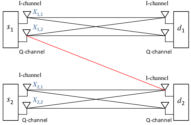
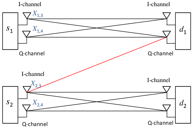
Refer to caption
(a) MIMO-S topology under (𝐀𝐒,𝐁𝐒)(\mathbf{A^{S}},\mathbf{B^{S}}).
Refer to caption
(b) MIMO-Z topology under (𝐀𝐙,𝐁𝐙)(\mathbf{A^{Z}},\mathbf{B^{Z}}).
Refer to caption
(c) MIMO-X topology under (𝐀𝐗,𝐁𝐗)(\mathbf{A^{X}},\mathbf{B^{X}}).
Fig. 6: End-to-end interference structures.

Although the 3-phase scheme described above achieves the optimal sum-DoF, i.e., 5/3, its performance can be improved for finite SNR by not insisting on creating the MIMO-S, MIMO-Z and MIMO-X topologies in the three phases. Instead, if only the coding pattern of transmit symbols in the three phases are preserved as shown in Figure 7, then s1s_{1} and s2s_{2} can achieve I⁡(X1,1,X1,2,X1,3,X1,4,X1,5,Y→11st,Y→12nd,Y→13rd)I(X_{1,1},X_{1,2},X_{1,3},X_{1,4},X_{1,5};\vec{Y}_{1}^{\text{1st}},\vec{Y}_{1}^{\text{2nd}},\vec{Y}_{1}^{\text{3rd}}) and I⁡(X2,1,X2,2,X2,3,X2,4,X2,5,Y→21st,Y→22nd,Y→23rd)I(X_{2,1},X_{2,2},X_{2,3},X_{2,4},X_{2,5};\vec{Y}_{2}^{\text{1st}},\vec{Y}_{2}^{\text{2nd}},\vec{Y}_{2}^{\text{3rd}}) respectively, where Y→i1st\vec{Y}_{i}^{\text{1st}}, Y→i2nd\vec{Y}_{i}^{\text{2nd}} and Y→i3rd\vec{Y}_{i}^{\text{3rd}} are the symbols received by did_{i} in the first, second and third phase respectively. More specifically, if we let X1,kX_{1,k}’s and X2,kX_{2,k}’s be independent random variables ∼𝒩⁡(0,P2)\sim\mathcal{N}(0,\frac{P}{2}) and let

𝒱={(𝐀,𝐁)∈ℝ2×2×ℝ2×2|||𝐀||≤P(‖H¯s1,u‖2+‖H¯s2,u‖2)​P+1,||𝐁||≤P(‖H¯s1,v‖2+‖H¯s2,v‖2)​P+1}\mathcal{V}\!=\!\left\{\!(\mathbf{A},\mathbf{B})\in\mathbb{R}^{2\times 2}\!\!\times\!\mathbb{R}^{2\times 2}\!\left|||\mathbf{A}||\leq\sqrt{\frac{P}{(||\bar{H}_{s_{1},u}||^{2}+||\bar{H}_{s_{2},u}||^{2})P+1}}\,,||\mathbf{B}||\leq\sqrt{\frac{P}{(||\bar{H}_{s_{1},v}||^{2}+||\bar{H}_{s_{2},v}||^{2})P+1}}\right.\right\}

be the set of relaying kernels that respect the power constraint for the relays where H¯a,b\bar{H}_{a,b} is defined in (116), then the sum-rate achievable by the 3-phase scheme not insisting on creating the three topologies is

R3-phase≜sup(𝐀1,𝐁1),(𝐀2,𝐁2),(𝐀3,𝐁3)∈𝒱{(R1,R2)|R1≤I⁡(X1,1,X1,2,X1,3,X1,4,X1,5,Y→11st,Y→12nd,Y→13rd),R2≤I⁡(X2,1,X2,2,X2,3,X2,4,X2,5,Y→21st,Y→22nd,Y→23rd)},R_{\text{3-phase}}\triangleq\sup_{(\mathbf{A}_{1},\mathbf{B}_{1}),(\mathbf{A}_{2},\mathbf{B}_{2}),(\mathbf{A}_{3},\mathbf{B}_{3})\in\mathcal{V}}\left\{(R_{1},R_{2})\left|\>\parbox[c]{224.03743pt}{$R_{1}\leq I(X_{1,1},X_{1,2},X_{1,3},X_{1,4},X_{1,5};\vec{Y}_{1}^{\text{1st}},\vec{Y}_{1}^{\text{2nd}},\vec{Y}_{1}^{\text{3rd}}),\\ R_{2}\leq I(X_{2,1},X_{2,2},X_{2,3},X_{2,4},X_{2,5};\vec{Y}_{2}^{\text{1st}},\vec{Y}_{2}^{\text{2nd}},\vec{Y}_{2}^{\text{3rd}})$}\right.\right\}, (119)

where (𝐀k,𝐁k)(\mathbf{A}_{k},\mathbf{B}_{k}) is the relaying kernel used in Phase kk. Although finding the optimal ((𝐀1,𝐁1),(𝐀2,𝐁2),(𝐀3,𝐁3))((\mathbf{A}_{1},\mathbf{B}_{1}),(\mathbf{A}_{2},\mathbf{B}_{2}),(\mathbf{A}_{3},\mathbf{B}_{3})) that maximizes R3-phaseR_{\text{3-phase}} is a non-convex optimization problem as shown in (119), we can still obtain in our simulation a heuristic sum-rate by first evaluating the closed form of the mutual information terms in (119) followed by conducting MATLAB constrained non-linear optimization initiated at the relaying kernels ((𝐀𝐒,𝐁𝐒),(𝐀𝐙,𝐁𝐙),(𝐀𝐗,𝐁𝐗))((\mathbf{A^{S}},\mathbf{B^{S}}),(\mathbf{A^{Z}},\mathbf{B^{Z}}),(\mathbf{A^{X}},\mathbf{B^{X}})) (cf. Figure 6).

Refer to caption
(a) Symbols transmitted in first phase.
Refer to caption
(b) Symbols transmitted in second phase.
Refer to caption
(c) Symbols transmitted in third phase.
Fig. 7: Patterns of transmit symbols in the three phases.

We now compare the achievable rate of our 3-phase scheme with other schemes in the literature. As for the benchmark, we consider two schemes: time-sharing (TDMA) and amplify-forward (AF) schemes. Under the TDMA scheme, the two sources transmit their messages in different time slots and the two relays forward the messages in different time slots in such a way that uu forwards only the message of s1s_{1} and vv forwards only the message of s2s_{2}. Under the AF scheme, the sources transmit the codewords consisting of complex symbols simultaneously and each relay multiplies its received codeword with a time-invariant complex scalar followed by transmitting the resultant codeword to the destinations. Upon receiving the complex codewords from the relays, each destination under the AF scheme decodes the message by treating interference as noise. For a finite PP, let

RTDMA=log2⁡(1+P)R_{\text{TDMA}}=\log_{2}(1+P)

be the sum-rate achievable by TDMA schemes, and let

RAF\displaystyle R_{\text{AF}} =maxα,β∈ℂ:|α|,|β|≤PP+1{log2(1+|g11|2​P|g12|2​P+|α|2+|β|2+1)\displaystyle=\max_{\alpha,\beta\in\mathbb{C}:|\alpha|,|\beta|\leq\sqrt{\frac{P}{P+1}}}\bigg\{\log_{2}\left(1+\frac{|g_{11}|^{2}P}{|g_{12}|^{2}P+|\alpha|^{2}+|\beta|^{2}+1}\right)
+log2(1+|g22|2​P|g21|2​P+|α|2+|β|2+1)}\displaystyle\qquad\hskip 115.63243pt+\log_{2}\left(1+\frac{|g_{22}|^{2}P}{|g_{21}|^{2}P+|\alpha|^{2}+|\beta|^{2}+1}\right)\bigg\}

be the sum-rate achievable by AF schemes, where α\alpha and β\beta are the amplifying scalars chosen by uu and vv respectively and gi​j≜hsj​u​hu​di​α+hsj​v​hv​di​βg_{ij}\triangleq h_{s_{j}u}h_{ud_{i}}\alpha+h_{s_{j}v}h_{vd_{i}}\beta is the end-to-end channel gain between sjs_{j} and did_{i}.

In addition, we also consider two recent schemes called compute-and-forward with aligned network diagonalization (CoF-AND) and precoded compute-and-forward with channel integer alignment (PCoF-CIA) [7] respectively. The main idea behind these schemes is to innovatively use lattice codes and transform the two-hop IC into a network defined on a finite field. Then, the relays cooperate to eliminate the end-to-end interference in the finite field domain by using aligned network diagonalization techniques [3] under CoF-AND and by using asymmetric complex signaling techniques [15] under PCoF-CIA. To facilitate discussion, let RCoF-ANDR_{\text{CoF-AND}} and RPCoF-CIAR_{\text{PCoF-CIA}} be the sum-rates achievable by CoF-AND and PCoF-CIA respectively.

Refer to caption
(a) r=0.5r=0.5.
Refer to caption
(b) r=1r=1.
Fig. 8: Comparison among TDMA, AF, CoF-AND, PCoF-CIA and our 3-phase linear schemes.

We now consider the numerical analysis of the aforementioned schemes for the network of Figure 5 and focus on two values of rr: r=1r=1 and r=0.5r=0.5 corresponding respectively to moderate and high interference regimes. In Figure 8, we plot for both regimes the average values of RTDMAR_{\text{TDMA}}, RAFR_{\text{AF}}, R3-phaseR_{\text{3-phase}} and max⁡{RCoF-AND,RPCoF-CIA}\max\{R_{\text{CoF-AND}},R_{\text{PCoF-CIA}}\} against power PP, where the average is obtained by Monte Carlo simulation which assumes that θa​b\theta_{ab}’s are i.i.d. phases uniformly distributed over [0,2​π][0,2\pi] (cf. Figure 5). In both cases, we note that our 3-phase linear scheme starts to outperform the other schemes at moderate SNR, particularly at about 15dB for r=0.5r=0.5 and 25dB for r=1r=1 as shown in Figures 8(a) and (b) respectively. Also, in both cases, the gap between the 3-phase scheme and the other schemes widens as PP increases, due to the fact that our scheme has a strictly higher sum-DoF. For the high interference regime (i.e., r=1r=1), we note that the performance of 3-phase scheme and the best of CoF-AND and PCoF-CIA schemes are very similar at moderate SNR (before 60dB). However, from the complexity perspective, since the 3-phase scheme only relies on simple linear operations over blocks of size 3, it can be more appealing.

VII Conclusion

In this paper, we analyzed the sum-DoF of the two-hop IC with real constant channel gains when relays are restricted to perform vector-linear schemes. We characterized the sum-DoF achievable by such schemes to be 4/3 for almost all values of real channel gains. We then extended the result to the case where each node has MM antennas. We showed that the linear sum-DoF in this setup is 2​M−2/32M-2/3 for almost all values of channel gains. Furthermore, we adapted this result to the case of complex channel gains and MM-antenna nodes, for which we characterized the sum-DoF to be 2​M−1/32M-1/3 for almost all values of complex channel gains. Finally, we analytically computed the rates achieved by our proposed scheme for the single-antenna two-hop IC with complex channel gains for different SNR values, and compared them with achievable rates of state-of-the-art schemes. Simulation results show that the proposed scheme is robust against changes in the interference strength, and outperforms state-of-the-art schemes even at moderate SNR.

This study can be extended in several directions. One direction could be to investigate the performance of linear schemes in more general two-unicast networks, such as those studied in [16, 17]. Another interesting direction is the study of linear schemes for general K×K×KK\times K\times K networks. A summary of current results is shown in Figure 9, where the xx-axis represents the number of users KK, and the yy-axis represents the achievable sum-DoF for the corresponding K×K×KK\times K\times K network (with complex channel gains). We already know, due to the result of [2], that the point (2,2) is achievable. More generally, we know that all points of the form (K,K)(K,K) are achievable due to the result of [3]. If we are restricted to amplify-forward schemes, then we know by the result of [18] that for a K×N×KK\times N\times K network, where N=K⁡(K−1)+1N=K(K-1)+1, all interference links can be canceled by appropriately choosing the relay coefficients, and thus KK sum-DoF is achievable. This implies that for the K×K×KK\times K\times K network we can achieve a sum-DoF of the order of K\sqrt{K}, by canceling as many interference links as possible. In this work, we showed that 5/3 sum-DoF is achievable for the 2×2×22\times 2\times 2 network. And so we ask: what can linear schemes achieve for general K×K×KK\times K\times K networks?

Refer to caption
Fig. 9: Summary of known results of interest for the achievable sum-DoF for general K×K×KK\times K\times K networks.

Appendix A Proof of Lemma 3

We first show that there exist four unique real numbers λ1′\lambda_{1}^{\prime}, λ2′\lambda_{2}^{\prime}, μ1′\mu_{1}^{\prime} and μ2′\mu_{2}^{\prime} which are functions of (𝐇1,𝐇2)(\mathbf{H}_{1},\mathbf{H}_{2}) such that

hs1​u​hu​d1​x+hs1​v​hv​d1​y=λ1′​(hs2​u​hu​d1​x+hs2​v​hv​d1​y)+λ2′​(hs1​u​hu​d2​x+hs1​v​hv​d2​y)h_{s_{1}u}h_{ud_{1}}x+h_{s_{1}v}h_{vd_{1}}y=\lambda_{1}^{\prime}(h_{s_{2}u}h_{ud_{1}}x+h_{s_{2}v}h_{vd_{1}}y)+\lambda_{2}^{\prime}(h_{s_{1}u}h_{ud_{2}}x+h_{s_{1}v}h_{vd_{2}}y) (120)

and

hs2​u​hu​d2​x+hs2​v​hv​d2​y=μ1′​(hs2​u​hu​d1​x+hs2​v​hv​d1​y)+μ2′​(hs1​u​hu​d2​x+hs1​v​hv​d2​y)h_{s_{2}u}h_{ud_{2}}x+h_{s_{2}v}h_{vd_{2}}y=\mu_{1}^{\prime}(h_{s_{2}u}h_{ud_{1}}x+h_{s_{2}v}h_{vd_{1}}y)+\mu_{2}^{\prime}(h_{s_{1}u}h_{ud_{2}}x+h_{s_{1}v}h_{vd_{2}}y) (121)

for all x∈ℝx\in\mathbb{R} and all y∈ℝy\in\mathbb{R}. The lemma will then follow from (36), (120) and (121) by letting λ1=λ1′\lambda_{1}=\lambda_{1}^{\prime}, λ2=λ2′\lambda_{2}=\lambda_{2}^{\prime}, μ1=μ1′\mu_{1}=\mu_{1}^{\prime} and μ2=μ2′\mu_{2}=\mu_{2}^{\prime}. Comparing coefficients of xx and yy on both sides of (120), we obtain the following matrix equation:

[hs2​u​hu​d1hs1​u​hu​d2hs2​v​hv​d1hs1​v​hv​d2]​[λ1′λ2′]=[hs1​u​hu​d1hs1​v​hv​d1].\left[\begin{array}[]{cc}h_{s_{2}u}h_{ud_{1}}&h_{s_{1}u}h_{ud_{2}}\\ h_{s_{2}v}h_{vd_{1}}&h_{s_{1}v}h_{vd_{2}}\end{array}\right]\left[\begin{array}[]{c}\lambda_{1}^{\prime}\\ \lambda_{2}^{\prime}\end{array}\right]=\left[\begin{array}[]{c}h_{s_{1}u}h_{ud_{1}}\\ h_{s_{1}v}h_{vd_{1}}\end{array}\right]. (122)

To facilitate discussion, let D=det​([hs2​u​hu​d1hs1​u​hu​d2hs2​v​hv​d1hs1​v​hv​d2])D={\rm\text{det}}\left(\left[\begin{array}[]{cc}h_{s_{2}u}h_{ud_{1}}&h_{s_{1}u}h_{ud_{2}}\\ h_{s_{2}v}h_{vd_{1}}&h_{s_{1}v}h_{vd_{2}}\end{array}\right]\right). Since D≠0D\neq 0 by condition (c-3), it follows from Cramer’s rule that the unique solution for (122) is

{λ1′=hs1​u​hs1​v​det​(𝐇2)D,λ2′=−hu​d1​hv​d1​det​(𝐇1)D.\begin{cases}\lambda_{1}^{\prime}=\frac{h_{s_{1}u}h_{s_{1}v}{\rm\text{det}}(\mathbf{H}_{2})}{D},\\ \lambda_{2}^{\prime}=\frac{-h_{ud_{1}}h_{vd_{1}}{\rm\text{det}}(\mathbf{H}_{1})}{D}.\end{cases} (123)

Substituting (123) into (120) followed by comparing coefficients of xx and yy on both sides of (120), we find that (120) is satisfied by λ1′\lambda_{1}^{\prime} and λ2′\lambda_{2}^{\prime}. Following similar procedures for obtaining λ1′\lambda_{1}^{\prime} and λ2′\lambda_{2}^{\prime} that satisfy (120), we obtain μ1′\mu_{1}^{\prime} and μ2′\mu_{2}^{\prime} that satisfy (121).

Appendix B Proof of Lemma 4

Let 𝐋\mathbf{L} be an n×nn\times n matrix. Expanding h⁡(Xn+Z1n,Yn+Z2n)h(X^{n}+Z_{1}^{n},Y^{n}+Z_{2}^{n}) in two different ways, we obtain

h⁡(Xn+Z1n)+h⁡(Yn+Z2n|Xn+Z1n)\displaystyle h(X^{n}+Z_{1}^{n})+h(Y^{n}+Z_{2}^{n}|X^{n}+Z_{1}^{n})
=h⁡(Yn+Z2n)+h⁡(Xn+Z1n|Yn+Z2n),\displaystyle\quad=h(Y^{n}+Z_{2}^{n})+h(X^{n}+Z_{1}^{n}|Y^{n}+Z_{2}^{n}),

which then implies that

h⁡(Xn+Z1n)−h⁡(Yn+Z2n)\displaystyle h(X^{n}+Z_{1}^{n})-h(Y^{n}+Z_{2}^{n})
=h⁡(Xn+Z1n|Yn+Z2n)−h⁡(Yn+Z2n|Xn+Z1n)\displaystyle=h(X^{n}+Z_{1}^{n}|Y^{n}+Z_{2}^{n})-h(Y^{n}+Z_{2}^{n}|X^{n}+Z_{1}^{n})
≤h⁡(Xn−𝐋​Yn+Z1n−𝐋​Z2n|Yn+Z2n)−h⁡(Yn+Z2n|Yn,Xn+Z1n)\displaystyle\leq h(X^{n}-\mathbf{L}Y^{n}+Z_{1}^{n}-\mathbf{L}Z_{2}^{n}|Y^{n}+Z_{2}^{n})-h(Y^{n}+Z_{2}^{n}|Y^{n},X^{n}+Z_{1}^{n})
≤h⁡(Xn−𝐋​Yn+Z1n−𝐋​Z2n|Yn+Z2n)−h⁡(Z2n|Yn,Xn+Z1n)\displaystyle\leq h(X^{n}-\mathbf{L}Y^{n}+Z_{1}^{n}-\mathbf{L}Z_{2}^{n}|Y^{n}+Z_{2}^{n})-h(Z_{2}^{n}|Y^{n},X^{n}+Z_{1}^{n})
=h⁡(Xn−𝐋​Yn+Z1n−𝐋​Z2n|Yn+Z2n)−h⁡(Z2n),\displaystyle=h(X^{n}-\mathbf{L}Y^{n}+Z_{1}^{n}-\mathbf{L}Z_{2}^{n}|Y^{n}+Z_{2}^{n})-h(Z_{2}^{n}),

where the last equality follows from the fact that Z1nZ_{1}^{n}, Z2nZ_{2}^{n} and (Xn,Yn)(X^{n},Y^{n}) are independent.

Appendix C Proof of Lemma 5

We need the following three propositions for proving Lemma 5.

Proposition 14

Let 𝒱\mathcal{V} be a finite set of ℓ×ℓ\ell\times\ell real matrices and let 𝕄\mathbb{M} be the set of real matrices. Then, there exist two mappings ϕ𝒱:𝒱→𝕄\phi_{\mathcal{V}}:\mathcal{V}\rightarrow\mathbb{M} and ψ𝒱:𝒱→𝕄\psi_{\mathcal{V}}:\mathcal{V}\rightarrow\mathbb{M} such that for any 𝐆∈𝒱\mathbf{G}\in\mathcal{V}, ϕ𝒱​(𝐆)\phi_{\mathcal{V}}(\mathbf{G}) is an invertible ℓ×ℓ\ell\times\ell matrix and ψ𝒱​(𝐆)\psi_{\mathcal{V}}(\mathbf{G}) is a rank⁡(𝐆)×ℓ{\rm{rank}}(\mathbf{G})\times\ell matrix that satisfy

{|det​(ϕ𝒱​(𝐆))|=1,andϕ𝒱​(𝐆)​𝐆=[ψ𝒱​(𝐆)𝟎(ℓ−rank⁡(𝐆))×ℓ].\begin{cases}|{\rm\text{det}}(\phi_{\mathcal{V}}(\mathbf{G}))|=1,~~\text{and}\\ \phi_{\mathcal{V}}(\mathbf{G})\mathbf{G}=\left[\begin{array}[]{c}\psi_{\mathcal{V}}(\mathbf{G})\\ \mathbf{0}^{(\ell-{\rm{rank}}(\mathbf{G}))\times\ell}\end{array}\right].\end{cases}

In addition, there exists a real number KK which is only a function of ℓ\ell and 𝒱\mathcal{V} such that KK is an upper bound on the magnitudes of the entries in each ϕ𝒱​(𝐆)\phi_{\mathcal{V}}(\mathbf{G}) and each ψ𝒱​(𝐆)\psi_{\mathcal{V}}(\mathbf{G}).

Proof:

Suppose 𝐆\mathbf{G} is a matrix in 𝒱\mathcal{V}. By linear algebra, there exists an invertible ℓ×ℓ\ell\times\ell matrix denoted by 𝐋𝐆\mathbf{L}_{\mathbf{G}} and a full-rank rank⁡(𝐆)×ℓ{\rm{rank}}(\mathbf{G})\times\ell matrix denoted by 𝐆∗\mathbf{G}^{*} such that |det​(𝐋𝐆)|=1|{\rm\text{det}}(\mathbf{L}_{\mathbf{G}})|=1 and 𝐋𝐆​𝐆=[𝐆∗𝟎(ℓ−rank⁡(𝐆))×ℓ]\mathbf{L}_{\mathbf{G}}\mathbf{G}=\left[\begin{array}[]{c}\mathbf{G}^{*}\\ \mathbf{0}^{(\ell-{\rm{rank}}(\mathbf{G}))\times\ell}\end{array}\right]. The lemma then follows by letting ϕ𝒱​(𝐆)=𝐋𝐆\phi_{\mathcal{V}}(\mathbf{G})=\mathbf{L}_{\mathbf{G}} and ψ𝒱​(𝐆)=𝐆∗\psi_{\mathcal{V}}(\mathbf{G})=\mathbf{G}^{*} for each 𝐆∈𝒱\mathbf{G}\in\mathcal{V} and letting KK be the maximum of max⁡{|g|:g​ is an entry in some ​ϕ𝒱​(𝐆)}\max\{|g|:g\text{ is an entry in some }\phi_{\mathcal{V}}(\mathbf{G})\} and max⁡{|g|:g​ is an entry in some ​ψ𝒱​(𝐆)}\max\{|g|:g\text{ is an entry in some }\psi_{\mathcal{V}}(\mathbf{G})\}. ∎

Proposition 15

For any xℓ∈ℝℓ×1x^{\ell}\in\mathbb{R}^{\ell\times 1} and any vector ϕ→∈ℝ1×ℓ\vec{\phi}\in\mathbb{R}^{1\times\ell} such that the magnitude of each entry of ϕ→\vec{\phi} is less than some K≥0K\geq 0, (ϕ→​xℓ)2≤ℓ2​K2​‖xℓ‖2(\vec{\phi}x^{\ell})^{2}\leq\ell^{2}K^{2}||x^{\ell}||^{2}.

Proof:

Let xℓ∈ℝℓ×1x^{\ell}\in\mathbb{R}^{\ell\times 1} and ϕ→∈ℝ1×ℓ\vec{\phi}\in\mathbb{R}^{1\times\ell} such that the magnitude of each entry of ϕ→\vec{\phi} is less than some K≥0K\geq 0. Since the magnitude of each entry of ϕ→\vec{\phi} is less than KK, |ϕ→​xℓ|≤K⁡(|x1|+|x2|+…+|xℓ|)|\vec{\phi}x^{\ell}|\leq K(|x_{1}|+|x_{2}|+\ldots+|x_{\ell}|) by triangle inequality, which then implies that

(ϕ→​xℓ)2\displaystyle(\vec{\phi}x^{\ell})^{2} ≤K2​(|x1|+|x2|+…+|xℓ|)2\displaystyle\leq K^{2}(|x_{1}|+|x_{2}|+\ldots+|x_{\ell}|)^{2}
≤K2​(ℓ​maxi∈{1,…,ℓ}​|xi|)2\displaystyle\leq K^{2}(\ell\max_{i\in\{1,\dots,\ell\}}|x_{i}|)^{2}
≤ℓ2​K2​(|x1|2+|x2|2+…+|xℓ|2)\displaystyle\leq\ell^{2}K^{2}(|x_{1}|^{2}+|x_{2}|^{2}+\ldots+|x_{\ell}|^{2})
≤ℓ2​K2​‖xℓ‖2.\displaystyle\leq\ell^{2}K^{2}||x^{\ell}||^{2}.

∎

Proposition 16

Let ℓ\ell be a natural number, u→\vec{u} be a standard basis vector in ℝ1×ℓ\mathbb{R}^{1\times\ell} and Λ1\Lambda_{1}, Λ2\Lambda_{2}, Ω1\Omega_{1}, Ω2\Omega_{2} and Ω3\Omega_{3} be five matrices in ℝℓ×ℓ\mathbb{R}^{\ell\times\ell}. In addition, let X1ℓX_{1}^{\ell}, X2ℓX_{2}^{\ell}, Z1ℓZ_{1}^{\ell}, Z2ℓZ_{2}^{\ell} and Z3ℓZ_{3}^{\ell} be five independent random vectors in ℝℓ×1\mathbb{R}^{\ell\times 1} such that ZiℓZ_{i}^{\ell} is ℓ\ell independent copies of 𝒩⁡(0,1)\mathcal{N}(0,1) for each i∈{1,2,3}i\in\{1,2,3\}. If there exists a real number KK such that KK is an upper bound on the magnitudes of the entries in Λ1\Lambda_{1}, Λ2\Lambda_{2}, Ω1\Omega_{1}, Ω2\Omega_{2} and Ω3\Omega_{3}, then there exists a real number κ\kappa which is only a function of KK and ℓ\ell such that

h⁡(u→​(Λ1​X1ℓ+Λ2​X2ℓ+Ω1​Z1ℓ+Ω2​Z2ℓ+Ω3​Z3ℓ))\displaystyle h(\vec{u}(\Lambda_{1}X_{1}^{\ell}+\Lambda_{2}X_{2}^{\ell}+\Omega_{1}Z_{1}^{\ell}+\Omega_{2}Z_{2}^{\ell}+\Omega_{3}Z_{3}^{\ell}))
≤log2⁡1+𝔼⁡[∑m=1ℓ(X1,m2+X2,m2)]/ℓ+κ\displaystyle\quad\leq\log_{2}\sqrt{1+{\rm\mathbb{E}}\left[\sum_{m=1}^{\ell}(X_{1,m}^{2}+X_{2,m}^{2})\right]/\ell}+\kappa (124)

and

h⁡(u→​(Ω1​Z1ℓ+Ω2​Z2ℓ+Ω3​Z3ℓ))≤κ.h(\vec{u}(\Omega_{1}Z_{1}^{\ell}+\Omega_{2}Z_{2}^{\ell}+\Omega_{3}Z_{3}^{\ell}))\leq\kappa. (125)
Proof:

Let K∈ℝK\in\mathbb{R} be an upper bound on the magnitudes of the entries in Λ1\Lambda_{1}, Λ2\Lambda_{2}, Ω1\Omega_{1}, Ω2\Omega_{2} and Ω3\Omega_{3}. Consider

𝔼⁡[(u→​(Λ1​X1ℓ+Λ2​X2ℓ+Ω1​Z1ℓ+Ω2​Z2ℓ+Ω3​Z3ℓ))2]\displaystyle{\rm\mathbb{E}}[(\vec{u}(\Lambda_{1}X_{1}^{\ell}+\Lambda_{2}X_{2}^{\ell}+\Omega_{1}Z_{1}^{\ell}+\Omega_{2}Z_{2}^{\ell}+\Omega_{3}Z_{3}^{\ell}))^{2}]
≤(a)2​𝔼​[(u→​(Λ1​X1ℓ+Λ2​X2ℓ))2+(u→​(Ω1​Z1ℓ+Ω2​Z2ℓ+Ω3​Z3ℓ))2]\displaystyle\quad\stackrel{{\scriptstyle\text{(a)}}}{{\leq}}2{\rm\mathbb{E}}[(\vec{u}(\Lambda_{1}X_{1}^{\ell}+\Lambda_{2}X_{2}^{\ell}))^{2}+(\vec{u}(\Omega_{1}Z_{1}^{\ell}+\Omega_{2}Z_{2}^{\ell}+\Omega_{3}Z_{3}^{\ell}))^{2}]
≤(b)2​ℓ2​K2​(𝔼⁡[‖X1ℓ+X2ℓ‖2]+𝔼⁡[‖Z1ℓ+Z2ℓ+Z3ℓ‖2])\displaystyle\quad\stackrel{{\scriptstyle\text{(b)}}}{{\leq}}2\ell^{2}K^{2}({\rm\mathbb{E}}[||X_{1}^{\ell}+X_{2}^{\ell}||^{2}]+{\rm\mathbb{E}}[||Z_{1}^{\ell}+Z_{2}^{\ell}+Z_{3}^{\ell}||^{2}])
≤(c)18​ℓ2​K2​(𝔼⁡[∑m=1ℓ(X1,m2+X2,m2)]+𝔼⁡[∑m=1ℓ(Z1,m2+Z2,m2+Z3,m2)])\displaystyle\quad\stackrel{{\scriptstyle\text{(c)}}}{{\leq}}18\ell^{2}K^{2}\left({\rm\mathbb{E}}\left[\sum_{m=1}^{\ell}(X_{1,m}^{2}+X_{2,m}^{2})\right]+{\rm\mathbb{E}}\left[\sum_{m=1}^{\ell}(Z_{1,m}^{2}+Z_{2,m}^{2}+Z_{3,m}^{2})\right]\right)
≤18​ℓ2​K2​(𝔼⁡[∑m=1ℓ(X1,m2+X2,m2)]+3​ℓ)\displaystyle\quad\leq 18\ell^{2}K^{2}\left({\rm\mathbb{E}}\left[\sum_{m=1}^{\ell}(X_{1,m}^{2}+X_{2,m}^{2})\right]+3\ell\right)
≤54​ℓ3​K2​(1+𝔼⁡[∑m=1ℓ(X1,m2+X2,m2)]/ℓ),\displaystyle\quad\leq 54\ell^{3}K^{2}\left(1+{\rm\mathbb{E}}\left[\sum_{m=1}^{\ell}(X_{1,m}^{2}+X_{2,m}^{2})\right]/\ell\right), (126)

where

  1. (a)

    follows from the fact that (a+b)2≤2​a2+2​b2(a+b)^{2}\leq 2a^{2}+2b^{2} for all real numbers aa and bb.

  2. (b)

    follows from Proposition 15.

  3. (c)

    follows from the fact that (a+b+c)2≤(3​max⁡{|a|,|b|,|c|})2≤9​(a2+b2+c2)(a+b+c)^{2}\leq(3\max\{|a|,|b|,|c|\})^{2}\leq 9(a^{2}+b^{2}+c^{2}) for all real numbers aa, bb and cc.

Since the differential entropy of a random variable XX is upper bounded by log2⁡2​π​e​𝔼​[X2]\log_{2}\sqrt{2\pi e{\rm\mathbb{E}}[X^{2}]}, it follows from (126) that (124) holds by choosing κ=log2⁡108​ℓ3​K2​π​e\kappa=\log_{2}\sqrt{108\ell^{3}K^{2}\pi e}. Following similar procedures for proving (124), we obtain (125) for the same κ\kappa chosen above. ∎

Proof:

Let

𝒢i​jℓ×ℓ={hsj​uhu​di𝐀+hsj​vhv​di𝐁|𝐀 and 𝐁 are in 𝒰ℓ×ℓ}\mathcal{G}_{ij}^{\ell\times\ell}=\left\{h_{s_{j}u}h_{ud_{i}}\mathbf{A}+h_{s_{j}v}h_{vd_{i}}\mathbf{B}\right|\left.\mathbf{A}\text{ and }\mathbf{B}\text{ are in }\mathcal{U}^{\ell\times\ell}\right\} (127)

be a finite set for each i,j∈{1,2}i,j\in\{1,2\}. Since 𝒰\mathcal{U} is finite, it follows from (127) that 𝒢12ℓ×ℓ\mathcal{G}_{12}^{\ell\times\ell} is finite, which then implies from Proposition 14 that there exist two mappings denoted by ϕ𝒢12\phi_{\mathcal{G}_{12}} and ψ𝒢12\psi_{\mathcal{G}_{12}} such that for any 𝐆𝟏𝟐∈𝒢12ℓ×ℓ\mathbf{G}_{\mathbf{12}}\in\mathcal{G}_{12}^{\ell\times\ell},

|det​(ϕ𝒢12​(𝐆𝟏𝟐))|=1,|{\rm\text{det}}(\phi_{\mathcal{G}_{12}}(\mathbf{G}_{\mathbf{12}}))|=1, (128)

and

ϕ𝒢12​(𝐆𝟏𝟐)​𝐆𝟏𝟐=[ψ𝒢12​(𝐆𝟏𝟐)𝟎(ℓ−rank⁡(𝐆𝟏𝟐))×ℓ].\phi_{\mathcal{G}_{12}}(\mathbf{G}_{\mathbf{12}})\mathbf{G}_{\mathbf{12}}=\left[\begin{array}[]{c}\psi_{\mathcal{G}_{12}}(\mathbf{G}_{\mathbf{12}})\\ \mathbf{0}^{(\ell-{\rm{rank}}(\mathbf{G}_{\mathbf{12}}))\times\ell}\end{array}\right]. (129)

In addition, there exists by Proposition 14 a real number K¯\bar{K} which is only a function of ℓ\ell and 𝒰\mathcal{U} such that K¯\bar{K} is an upper bound on the magnitudes of the entries in each ϕ𝒢12​(𝐆𝟏𝟐)\phi_{\mathcal{G}_{12}}(\mathbf{G}_{\mathbf{12}}) and each ψ𝒢12​(𝐆𝟏𝟐)\psi_{\mathcal{G}_{12}}(\mathbf{G}_{\mathbf{12}}). For each k∈{1,2,…,n}k\in\{1,2,\ldots,n\}, consider

h⁡(𝐆𝟏𝟐,k​(λ1​X1,ℓk−1+X2,ℓk−1)+Z1,ℓk−λ2​Z2,ℓk)\displaystyle h(\mathbf{G}_{\mathbf{12},k}(\lambda_{1}X_{1,\ell_{k-1}}+X_{2,\ell_{k-1}})+Z_{1,\ell_{k}}-\lambda_{2}Z_{2,\ell_{k}})
=(a)h⁡(ϕ𝒢12​(𝐆𝟏𝟐,k)​(𝐆𝟏𝟐,k​(λ1​X1,ℓk−1+X2,ℓk−1)+Z1,ℓk−λ2​Z2,ℓk))\displaystyle\stackrel{{\scriptstyle\text{(a)}}}{{=}}h(\phi_{\mathcal{G}_{12}}(\mathbf{G}_{\mathbf{12},k})(\mathbf{G}_{\mathbf{12},k}(\lambda_{1}X_{1,\ell_{k-1}}+X_{2,\ell_{k-1}})+Z_{1,\ell_{k}}-\lambda_{2}Z_{2,\ell_{k}}))
=(129)h⁡([ψ𝒢12​(𝐆𝟏𝟐,k)𝟎(ℓ−rank⁡(𝐆𝟏𝟐,k))×ℓ]​(λ1​X1,ℓk−1+X2,ℓk−1)+ϕ𝒢12​(𝐆𝟏𝟐,k)​(Z1,ℓk−λ2​Z2,ℓk)),\displaystyle\stackrel{{\scriptstyle\text{\eqref{functionsPhiPsi12}}}}{{=}}h\left(\left[\begin{array}[]{c}\psi_{\mathcal{G}_{12}}(\mathbf{G}_{\mathbf{12},k})\\ \mathbf{0}^{(\ell-{\rm{rank}}(\mathbf{G}_{\mathbf{12},k}))\times\ell}\end{array}\right](\lambda_{1}X_{1,\ell_{k-1}}+X_{2,\ell_{k-1}})+\phi_{\mathcal{G}_{12}}(\mathbf{G}_{\mathbf{12},k})(Z_{1,\ell_{k}}-\lambda_{2}Z_{2,\ell_{k}})\right),

where (a) follows from (128) and the fact that h⁡(𝐋​Xℓ)=h⁡(Xℓ)+log2⁡|det​(𝐋)|h(\mathbf{L}X^{\ell})=h(X^{\ell})+\log_{2}|{\rm\text{det}}(\mathbf{L})| for any invertible matrix 𝐋\mathbf{L}. To facilitate discussion, let

𝐈kleft=[𝐈rank⁡(𝐆𝟏𝟐,k)𝟎rank⁡(𝐆𝟏𝟐,k)×(ℓ−rank⁡(𝐆𝟏𝟐,k))]\mathbf{I}_{k}^{\text{left}}=\left[\begin{array}[]{cc}\mathbf{I}_{{\rm{rank}}(\mathbf{G}_{\mathbf{12},k})}&\mathbf{0}^{{\rm{rank}}(\mathbf{G}_{\mathbf{12},k})\times(\ell-{\rm{rank}}(\mathbf{G}_{\mathbf{12},k}))}\end{array}\right] (132)

and

𝐈kright=[𝟎(ℓ−rank⁡(𝐆𝟏𝟐,k))×rank⁡(𝐆𝟏𝟐,k)𝐈(ℓ−rank⁡(𝐆𝟏𝟐,k))]\mathbf{I}_{k}^{\text{right}}=\left[\begin{array}[]{cc}\mathbf{0}^{(\ell-{\rm{rank}}(\mathbf{G}_{\mathbf{12},k}))\times{\rm{rank}}(\mathbf{G}_{\mathbf{12},k})}&\mathbf{I}^{(\ell-{\rm{rank}}(\mathbf{G}_{\mathbf{12},k}))}\end{array}\right]

such that [𝐈kleft𝐈kright]=𝐈ℓ\left[\begin{array}[]{c}\mathbf{I}_{k}^{\text{left}}\\ \mathbf{I}_{k}^{\text{right}}\end{array}\right]=\mathbf{I}_{\ell}. Then, it follows from (C) that for each k∈{1,2,…,n}k\in\{1,2,\ldots,n\},

h⁡([ψ𝒢12​(𝐆𝟏𝟐,k)𝟎(ℓ−rank⁡(𝐆𝟏𝟐,k))×ℓ]​(λ1​X1,ℓk−1+X2,ℓk−1)+ϕ𝒢12​(𝐆𝟏𝟐,k)​(Z1,ℓk−λ2​Z2,ℓk))\displaystyle h\left(\left[\begin{array}[]{c}\psi_{\mathcal{G}_{12}}(\mathbf{G}_{\mathbf{12},k})\\ \mathbf{0}^{(\ell-{\rm{rank}}(\mathbf{G}_{\mathbf{12},k}))\times\ell}\end{array}\right](\lambda_{1}X_{1,\ell_{k-1}}+X_{2,\ell_{k-1}})+\phi_{\mathcal{G}_{12}}(\mathbf{G}_{\mathbf{12},k})(Z_{1,\ell_{k}}-\lambda_{2}Z_{2,\ell_{k}})\right)
≤h⁡(𝐈kleft​([ψ𝒢12​(𝐆𝟏𝟐,k)𝟎ℓ×(ℓ−rank⁡(𝐆𝟏𝟐,k))×ℓ]​(λ1​X1,ℓk−1+X2,ℓk−1)+ϕ𝒢12​(𝐆𝟏𝟐,k)​(Z1,ℓk−λ2​Z2,ℓk)))\displaystyle\quad\leq h\left(\mathbf{I}_{k}^{\text{left}}\left(\left[\begin{array}[]{c}\psi_{\mathcal{G}_{12}}(\mathbf{G}_{\mathbf{12},k})\\ \mathbf{0}^{\ell\times(\ell-{\rm{rank}}(\mathbf{G}_{\mathbf{12},k}))\times\ell}\end{array}\right](\lambda_{1}X_{1,\ell_{k-1}}+X_{2,\ell_{k-1}})+\phi_{\mathcal{G}_{12}}(\mathbf{G}_{\mathbf{12},k})(Z_{1,\ell_{k}}-\lambda_{2}Z_{2,\ell_{k}})\right)\right)
+h⁡(𝐈kright​ϕ𝒢12​(𝐆𝟏𝟐,k)​(Z1,ℓk−λ2​Z2,ℓk))\displaystyle\qquad+h\left(\mathbf{I}_{k}^{\text{right}}\phi_{\mathcal{G}_{12}}(\mathbf{G}_{\mathbf{12},k})(Z_{1,\ell_{k}}-\lambda_{2}Z_{2,\ell_{k}})\right)
≤rank⁡(𝐆𝟏𝟐,k)​log2​1+Pk−1/ℓ+κ\displaystyle\quad\leq{\rm{rank}}(\mathbf{G}_{\mathbf{12},k})\log_{2}\sqrt{1+P_{k-1}/\ell}+\kappa (137)

for some κ\kappa that does not depend on nn and PP, where the last inequality follows from Proposition 16 by setting Λ1=λ1​[ψ𝒢12​(𝐆𝟏𝟐,k)𝟎ℓ×(ℓ−rank⁡(𝐆𝟏𝟐,k))×ℓ]\Lambda_{1}=\lambda_{1}\left[\begin{array}[]{c}\psi_{\mathcal{G}_{12}}(\mathbf{G}_{\mathbf{12},k})\\ \mathbf{0}^{\ell\times(\ell-{\rm{rank}}(\mathbf{G}_{\mathbf{12},k}))\times\ell}\end{array}\right], Λ2=[ψ𝒢12​(𝐆𝟏𝟐,k)𝟎ℓ×(ℓ−rank⁡(𝐆𝟏𝟐,k))×ℓ]\Lambda_{2}=\left[\begin{array}[]{c}\psi_{\mathcal{G}_{12}}(\mathbf{G}_{\mathbf{12},k})\\ \mathbf{0}^{\ell\times(\ell-{\rm{rank}}(\mathbf{G}_{\mathbf{12},k}))\times\ell}\end{array}\right], Ω1=ϕ𝒢12​(𝐆𝟏𝟐,k)\Omega_{1}=\phi_{\mathcal{G}_{12}}(\mathbf{G}_{\mathbf{12},k}), Ω2=−λ2​ϕ𝒢12​(𝐆𝟏𝟐,k)\Omega_{2}=-\lambda_{2}\phi_{\mathcal{G}_{12}}(\mathbf{G}_{\mathbf{12},k}), Ω3=𝟎ℓ×ℓ\Omega_{3}=\mathbf{0}^{\ell\times\ell} and K=max⁡{K¯,|λ1|​K¯,|λ2|​K¯}K=\max\{\bar{K},|\lambda_{1}|\bar{K},|\lambda_{2}|\bar{K}\}. Following similar procedures for deriving (137), we obtain that there exists some κ′\kappa^{\prime} that do not depend on nn and PP such that

h⁡(𝐆𝟐𝟏,k​(X1,ℓk−1+μ2​X2,ℓk−1)+Z2,ℓk−μ1​Z1,ℓk)\displaystyle h(\mathbf{G}_{\mathbf{21},k}(X_{1,\ell_{k-1}}+\mu_{2}X_{2,\ell_{k-1}})+Z_{2,\ell_{k}}-\mu_{1}Z_{1,\ell_{k}})
≤rank⁡(𝐆𝟐𝟏,k)​log2​1+Pk−1/ℓ+κ′\displaystyle\quad\leq{\rm{rank}}(\mathbf{G}_{\mathbf{21},k})\log_{2}\sqrt{1+P_{k-1}/\ell}+\kappa^{\prime}

for each k∈{1,2,…,n}k\in\{1,2,\ldots,n\}. ∎

Appendix D Proof of Lemma 6

We need the following proposition to prove Lemma 6.

Proposition 17

Let 𝒱\mathcal{V} be a finite set of ℓ×ℓ\ell\times\ell real matrices and let 𝕄\mathbb{M} denote the set of real matrices. Then, there exist three mappings ρ𝒱:𝒱→𝕄\rho_{\mathcal{V}}:\mathcal{V}\rightarrow\mathbb{M}, σ𝒱:𝒱→𝕄\sigma_{\mathcal{V}}:\mathcal{V}\rightarrow\mathbb{M} and τ𝒱:𝒱→𝕄\tau_{\mathcal{V}}:\mathcal{V}\rightarrow\mathbb{M} such that for any 𝐆∈𝒱\mathbf{G}\in\mathcal{V}, ρ𝒱​(𝐆)\rho_{\mathcal{V}}(\mathbf{G}) is an (ℓ−rank⁡(𝐆))×ℓ(\ell-{\rm{rank}}(\mathbf{G}))\times\ell matrix, σ𝒱​(𝐆)\sigma_{\mathcal{V}}(\mathbf{G}) is an ℓ×ℓ\ell\times\ell matrix and τ𝒱​(𝐆)\tau_{\mathcal{V}}(\mathbf{G}) is an ℓ×ℓ\ell\times\ell matrix that satisfy

𝐈ℓ=σ𝒱​(𝐆)​𝐆+τ𝒱​(𝐆)​[ρ𝒱​(𝐆)𝟎rank⁡(𝐆)×ℓ].\mathbf{I}_{\ell}=\sigma_{\mathcal{V}}(\mathbf{G})\mathbf{G}+\tau_{\mathcal{V}}(\mathbf{G})\left[\begin{array}[]{c}\rho_{\mathcal{V}}(\mathbf{G})\\ \mathbf{0}^{{\rm{rank}}(\mathbf{G})\times\ell}\end{array}\right].

In addition, there exists a real number KK which is only a function of ℓ\ell and 𝒱\mathcal{V} such that KK is an upper bound on the magnitudes of the entries in each ρ𝒱​(𝐆)\rho_{\mathcal{V}}(\mathbf{G}), each σ𝒱​(𝐆)\sigma_{\mathcal{V}}(\mathbf{G}) and each τ𝒱​(𝐆)\tau_{\mathcal{V}}(\mathbf{G}).

Proof:

Suppose 𝐆\mathbf{G} is a matrix in 𝒱\mathcal{V}. By linear algebra, there exists an (ℓ−rank⁡(𝐆))×ℓ(\ell-{\rm{rank}}(\mathbf{G}))\times\ell matrix 𝐆⊥\mathbf{G}^{\bot} such that the rows of 𝐆\mathbf{G} and 𝐆⊥\mathbf{G}^{\bot} together span ℝℓ\mathbb{R}^{\ell}. In other words, there exist an ℓ×ℓ\ell\times\ell matrix 𝛀𝟏\mathbf{\Omega_{1}} and an ℓ×ℓ\ell\times\ell matrix 𝛀𝟐\mathbf{\Omega_{2}} such that 𝐈ℓ=𝛀𝟏​𝐆+𝛀𝟐​[𝐆⊥𝟎rank⁡(𝐆)×ℓ]\mathbf{I}_{\ell}=\mathbf{\Omega_{1}}\mathbf{G}+\mathbf{\Omega_{2}}\left[\begin{array}[]{c}\mathbf{G}^{\bot}\\ \mathbf{0}^{{\rm{rank}}(\mathbf{G})\times\ell}\end{array}\right]. The lemma then follows by letting ρ𝒱​(𝐆)=𝐆⊥\rho_{\mathcal{V}}(\mathbf{G})=\mathbf{G}^{\bot}, σ𝒱​(𝐆)=𝛀𝟏\sigma_{\mathcal{V}}(\mathbf{G})=\mathbf{\Omega_{1}} and τ𝒱​(𝐆)=𝛀𝟐\tau_{\mathcal{V}}(\mathbf{G})=\mathbf{\Omega_{2}} for each 𝐆∈𝒱\mathbf{\mathbf{G}}\in\mathcal{V} and letting KK be the maximum of max⁡{|g|:g​ is an entry in some ​ρ𝒱​(𝐆)}\max\{|g|:g\text{ is an entry in some }\rho_{\mathcal{V}}(\mathbf{G})\}, max⁡{|g|:g​ is an entry in some ​σ𝒱​(𝐆)}\max\{|g|:g\text{ is an entry in some }\sigma_{\mathcal{V}}(\mathbf{G})\} and max⁡{|g|:g​ is an entry in some ​τ𝒱​(𝐆)}\max\{|g|:g\text{ is an entry in some }\tau_{\mathcal{V}}(\mathbf{G})\}. ∎

Proof:

Let 𝒢i​jℓ×ℓ\mathcal{G}_{ij}^{\ell\times\ell} be the set defined in (127) for each i,j∈{1,2}i,j\in\{1,2\}. Since 𝒰\mathcal{U} is finite, it follows that 𝒢i​jℓ×ℓ\mathcal{G}_{ij}^{\ell\times\ell} is finite for all i,j∈{1,2}i,j\in\{1,2\}, which implies that there exists a real number K∗K^{*} which is only a function of 𝒰\mathcal{U} such that K∗K^{*} is an upper bound on the magnitudes of the entries in each 𝐆𝐢𝐣∈𝒢i​jℓ×ℓ\mathbf{G}_{\mathbf{ij}}\in\mathcal{G}_{ij}^{\ell\times\ell} for all i,j∈{1,2}i,j\in\{1,2\}. Then,

h⁡(Y~1,ℓk)\displaystyle h(\tilde{Y}_{1,\ell_{k}}) =(39)h⁡(𝐆𝟏𝟏,k​X1,ℓk+𝐆𝟏𝟐,k​X2,ℓk+Z1,ℓk)\displaystyle\stackrel{{\scriptstyle\eqref{tildeY1}}}{{=}}h(\mathbf{G}_{\mathbf{11},k}X_{1,\ell_{k}}+\mathbf{G}_{\mathbf{12},k}X_{2,\ell_{k}}+Z_{1,\ell_{k}})
≤ℓ​log2​1+Pk−1/ℓ+κ\displaystyle\leq\ell\log_{2}\sqrt{1+P_{k-1}/\ell}+\kappa

for some κ\kappa that does not depend on nn and PP, where the inequality follows from Proposition 16 by setting Λ1=𝐆𝟏𝟏,k\Lambda_{1}=\mathbf{G}_{\mathbf{11},k}, Λ2=𝐆𝟏𝟐,k\Lambda_{2}=\mathbf{G}_{\mathbf{12},k}, Ω1=𝐈ℓ\Omega_{1}=\mathbf{I}_{\ell}, Ω2=Ω3=𝟎ℓ×ℓ\Omega_{2}=\Omega_{3}=\mathbf{0}^{\ell\times\ell} and K=max⁡{K∗,1}K=\max\{K^{*},1\}.

In addition, it follows from (127) that 𝒢12ℓ×ℓ\mathcal{G}_{12}^{\ell\times\ell} is finite, which then implies from Proposition 17 that there exist three mappings denoted by ρ𝒢12\rho_{\mathcal{G}_{12}}, σ𝒢12\sigma_{\mathcal{G}_{12}} and τ𝒢12\tau_{\mathcal{G}_{12}} respectively such that for any 𝐆𝟏𝟐∈𝒢12ℓ×ℓ\mathbf{G}_{\mathbf{12}}\in\mathcal{G}_{12}^{\ell\times\ell},

𝐈ℓ=σ𝒢12​(𝐆𝟏𝟐)​𝐆𝟏𝟐+τ𝒢12​(𝐆𝟏𝟐)​[ρ𝒢12​(𝐆𝟏𝟐)𝟎rank⁡(𝐆𝟏𝟐)×ℓ].\mathbf{I}_{\ell}=\sigma_{\mathcal{G}_{12}}(\mathbf{G}_{\mathbf{12}})\mathbf{G}_{\mathbf{12}}+\tau_{\mathcal{G}_{12}}(\mathbf{G}_{\mathbf{12}})\left[\begin{array}[]{c}\rho_{\mathcal{G}_{12}}(\mathbf{G}_{\mathbf{12}})\\ \mathbf{0}^{{\rm{rank}}(\mathbf{G}_{\mathbf{12}})\times\ell}\end{array}\right]. (138)

Let K¯\bar{K} be the real number in Proposition 17 which is only a function of ℓ\ell and 𝒰\mathcal{U} such that K¯\bar{K} is an upper bound on the magnitudes of the entries in each ρ𝒢12​(𝐆𝟏𝟐)\rho_{\mathcal{G}_{12}}(\mathbf{G}_{\mathbf{12}}), each σ𝒢12​(𝐆𝟏𝟐)\sigma_{\mathcal{G}_{12}}(\mathbf{G}_{\mathbf{12}}) and each τ𝒢12​(𝐆𝟏𝟐)\tau_{\mathcal{G}_{12}}(\mathbf{G}_{\mathbf{12}}). Let Z¯2ℓ​n\bar{Z}_{2}^{\ell n} be ℓ​n\ell n copies of 𝒩⁡(0,1)\mathcal{N}(0,1) such that Z¯2ℓ​n\bar{Z}_{2}^{\ell n}, X1ℓ​nX_{1}^{\ell n}, X2ℓ​nX_{2}^{\ell n}, Z1ℓ​nZ_{1}^{\ell n} and Z2ℓ​nZ_{2}^{\ell n} are independent, and let

Y→2,k′=[ρ𝒢12​(𝐆𝟏𝟐,k)𝟎rank⁡(𝐆𝟏𝟐,k)×ℓ]​X2,ℓk−1+Z¯2,ℓk.\vec{Y}_{2,k}^{\prime}=\left[\begin{array}[]{c}\rho_{\mathcal{G}_{12}}(\mathbf{G}_{\mathbf{12},k})\\ \mathbf{0}^{{\rm{rank}}(\mathbf{G}_{\mathbf{12},k})\times\ell}\end{array}\right]X_{2,\ell_{k-1}}+\bar{Z}_{2,\ell_{k}}. (139)

Using (138) and (139), we obtain

σ𝒢12​(𝐆𝟏𝟐,k)​(𝐆𝟏𝟐,k​X2,ℓk−1+Z1,ℓk)+τ𝒢12​(𝐆𝟏𝟐,k)​Y→2,k′\displaystyle\sigma_{\mathcal{G}_{12}}(\mathbf{G}_{\mathbf{12},k})(\mathbf{G}_{\mathbf{12},k}X_{2,\ell_{k-1}}+Z_{1,\ell_{k}})+\tau_{\mathcal{G}_{12}}(\mathbf{G}_{\mathbf{12},k})\vec{Y}_{2,k}^{\prime}\,
=X2,ℓk−1+σ𝒢12​(𝐆𝟏𝟐,k)​Z1,ℓk+τ𝒢12​(𝐆𝟏𝟐,k)​Z¯2,ℓk.\displaystyle\quad=X_{2,\ell_{k-1}}+\sigma_{\mathcal{G}_{12}}(\mathbf{G}_{\mathbf{12},k})Z_{1,\ell_{k}}+\tau_{\mathcal{G}_{12}}(\mathbf{G}_{\mathbf{12},k})\bar{Z}_{2,\ell_{k}}. (140)

Then, for each k∈{1,2,…,n}k\in\{1,2,\ldots,n\},

h⁡(𝐆𝟐𝟐,k​X2,ℓk−1+Z2,ℓk|𝐆𝟏𝟐,k​X2,ℓk−1+Z1,ℓk)\displaystyle h(\mathbf{G}_{\mathbf{22},k}X_{2,\ell_{k-1}}+Z_{2,\ell_{k}}|\mathbf{G}_{\mathbf{12},k}X_{2,\ell_{k-1}}+Z_{1,\ell_{k}})
=h⁡(𝐆𝟐𝟐,k​X2,ℓk−1+Z2,ℓk|𝐆𝟏𝟐,k​X2,ℓk−1+Z1,ℓk,Y→2,k′)+I⁡(𝐆𝟐𝟐,k​X2,ℓk−1+Z2,ℓk;Y→2,k′|𝐆𝟏𝟐,k​X2,ℓk−1+Z1,ℓk)\displaystyle\quad=h(\mathbf{G}_{\mathbf{22},k}X_{2,\ell_{k-1}}+Z_{2,\ell_{k}}|\mathbf{G}_{\mathbf{12},k}X_{2,\ell_{k-1}}+Z_{1,\ell_{k}},\vec{Y}_{2,k}^{\prime})+I(\mathbf{G}_{\mathbf{22},k}X_{2,\ell_{k-1}}+Z_{2,\ell_{k}};\vec{Y}_{2,k}^{\prime}|\mathbf{G}_{\mathbf{12},k}X_{2,\ell_{k-1}}+Z_{1,\ell_{k}})
≤h⁡(𝐆𝟐𝟐,k​X2,ℓk−1+Z2,ℓk|𝐆𝟏𝟐,k​X2,ℓk−1+Z1,ℓk,Y→2,k′)+h⁡(Y→2,k′)−h⁡(Y→2,k′|X2,ℓk−1,Z1,ℓk,Z2,ℓk)\displaystyle\quad\leq h(\mathbf{G}_{\mathbf{22},k}X_{2,\ell_{k-1}}+Z_{2,\ell_{k}}|\mathbf{G}_{\mathbf{12},k}X_{2,\ell_{k-1}}+Z_{1,\ell_{k}},\vec{Y}_{2,k}^{\prime})+h(\vec{Y}_{2,k}^{\prime})-h(\vec{Y}_{2,k}^{\prime}|X_{2,\ell_{k-1}},Z_{1,\ell_{k}},Z_{2,\ell_{k}})
=(a)h⁡(𝐆𝟐𝟐,k​X2,ℓk−1+Z2,ℓk|𝐆𝟏𝟐,k​X2,ℓk−1+Z1,ℓk,Y→2,k′)+h⁡(Y→2,k′)−h⁡(Z¯2,ℓk)\displaystyle\quad\stackrel{{\scriptstyle\text{(a)}}}{{=}}h(\mathbf{G}_{\mathbf{22},k}X_{2,\ell_{k-1}}+Z_{2,\ell_{k}}|\mathbf{G}_{\mathbf{12},k}X_{2,\ell_{k-1}}+Z_{1,\ell_{k}},\vec{Y}_{2,k}^{\prime})+h(\vec{Y}_{2,k}^{\prime})-h(\bar{Z}_{2,\ell_{k}})
≤(b)h⁡(Y→2,k′)+h⁡(𝐆𝟐𝟐,k​X2,ℓk−1+Z2,ℓk|𝐆𝟏𝟐,k​X2,ℓk−1+Z1,ℓk,Y→2,k′)\displaystyle\quad\stackrel{{\scriptstyle\text{(b)}}}{{\leq}}h(\vec{Y}_{2,k}^{\prime})+h(\mathbf{G}_{\mathbf{22},k}X_{2,\ell_{k-1}}+Z_{2,\ell_{k}}|\mathbf{G}_{\mathbf{12},k}X_{2,\ell_{k-1}}+Z_{1,\ell_{k}},\vec{Y}_{2,k}^{\prime})
≤h⁡(Y→2,k′)+h⁡(𝐆𝟐𝟐,k​X2,ℓk−1+Z2,ℓk−𝐆𝟐𝟐,k​(σ𝒢12​(𝐆𝟏𝟐,k)​(𝐆𝟏𝟐,k​X2,ℓk−1+Z1,ℓk)+τ𝒢12​(𝐆𝟏𝟐,k)​Y→2,k′))\displaystyle\quad\leq h(\vec{Y}_{2,k}^{\prime})+h(\mathbf{G}_{\mathbf{22},k}X_{2,\ell_{k-1}}+Z_{2,\ell_{k}}-\mathbf{G}_{\mathbf{22},k}(\sigma_{\mathcal{G}_{12}}(\mathbf{G}_{\mathbf{12},k})(\mathbf{G}_{\mathbf{12},k}X_{2,\ell_{k-1}}+Z_{1,\ell_{k}})+\tau_{\mathcal{G}_{12}}(\mathbf{G}_{\mathbf{12},k})\vec{Y}_{2,k}^{\prime}))
≤(140)h⁡(Y→2,k′)+h⁡(Z2,ℓk−𝐆𝟐𝟐,k​σ𝒢12​(𝐆𝟏𝟐,k)​Z1,ℓk−𝐆𝟐𝟐,k​τ𝒢12​(𝐆𝟏𝟐,k)​Z¯2,ℓk),\displaystyle\quad\stackrel{{\scriptstyle\eqref{lemmaDifferentialEntropyBound2ProofTemp}}}{{\leq}}h(\vec{Y}_{2,k}^{\prime})+h(Z_{2,\ell_{k}}-\mathbf{G}_{\mathbf{22},k}\,\sigma_{\mathcal{G}_{12}}(\mathbf{G}_{\mathbf{12},k})Z_{1,\ell_{k}}-\mathbf{G}_{\mathbf{22},k}\,\tau_{\mathcal{G}_{12}}(\mathbf{G}_{\mathbf{12},k})\bar{Z}_{2,\ell_{k}}),

where

  1. (a)

    follows from (139) and the fact that Z¯2ℓ​n\bar{Z}_{2}^{\ell n}, X2ℓ​nX_{2}^{\ell n}, Z1ℓ​nZ_{1}^{\ell n} and Z2ℓ​nZ_{2}^{\ell n} are independent.

  2. (b)

    follows from the fact that {Z¯2,m}m=1ℓ​n\{\bar{Z}_{2,m}\}_{m=1}^{\ell n} are independent and the differential entropy of 𝒩⁡(0,1)\mathcal{N}(0,1) is positive.

For each k∈{1,2,…,n}k\in\{1,2,\ldots,n\},

h⁡(Y→2,k′)\displaystyle h(\vec{Y}_{2,k}^{\prime}) =(139)h⁡([ρ𝒢12​(𝐆𝟏𝟐,k)𝟎rank⁡(𝐆𝟏𝟐,k)×ℓ]​X2,ℓk−1+Z¯2,ℓk)\displaystyle\stackrel{{\scriptstyle\eqref{Y2Prime}}}{{=}}h\left(\left[\begin{array}[]{c}\rho_{\mathcal{G}_{12}}(\mathbf{G}_{\mathbf{12},k})\\ \mathbf{0}^{{\rm{rank}}(\mathbf{G}_{\mathbf{12},k})\times\ell}\end{array}\right]X_{2,\ell_{k-1}}+\bar{Z}_{2,\ell_{k}}\right)
≤(a)h⁡(𝐈kleft​([ρ𝒢12​(𝐆𝟏𝟐,k)𝟎rank⁡(𝐆𝟏𝟐,k)×ℓ]​X2,ℓk−1+Z¯2,ℓk))+∑m=ℓ−rank⁡(𝐆𝟏𝟐)+1ℓh⁡(Z¯2,ℓ⁡(k−1)+m)\displaystyle\stackrel{{\scriptstyle\text{(a)}}}{{\leq}}h\left(\mathbf{I}_{k}^{\text{left}}\left(\left[\begin{array}[]{c}\rho_{\mathcal{G}_{12}}(\mathbf{G}_{\mathbf{12},k})\\ \mathbf{0}^{{\rm{rank}}(\mathbf{G}_{\mathbf{12},k})\times\ell}\end{array}\right]X_{2,\ell_{k-1}}+\bar{Z}_{2,\ell_{k}}\right)\right)+\sum_{m=\ell-{\rm{rank}}(\mathbf{G}_{\mathbf{12}})+1}^{\ell}h(\bar{Z}_{2,\ell(k-1)+m})
≤(b)(ℓ−rank⁡(𝐆𝟏𝟐,k))​log2​1+Pk−1/ℓ+κ\displaystyle\stackrel{{\scriptstyle\text{(b)}}}{{\leq}}(\ell-{\rm{rank}}(\mathbf{G}_{\mathbf{12},k}))\log_{2}\sqrt{1+P_{k-1}/\ell}+\kappa

and

h⁡(Z2,ℓk−𝐆𝟐𝟐,k​σ𝒢12​(𝐆𝟏𝟐,k)​Z1,ℓk−𝐆𝟐𝟐,k​τ𝒢12​(𝐆𝟏𝟐,k)​Z¯2,ℓk)\displaystyle h(Z_{2,\ell_{k}}-\mathbf{G}_{\mathbf{22},k}\,\sigma_{\mathcal{G}_{12}}(\mathbf{G}_{\mathbf{12},k})Z_{1,\ell_{k}}-\mathbf{G}_{\mathbf{22},k}\,\tau_{\mathcal{G}_{12}}(\mathbf{G}_{\mathbf{12},k})\bar{Z}_{2,\ell_{k}})
≤(c)ℓ​log2​1+Pk−1/ℓ+κ′\displaystyle\stackrel{{\scriptstyle\text{(c)}}}{{\leq}}\ell\log_{2}\sqrt{1+P_{k-1}/\ell}+\kappa^{\prime}

for some κ\kappa and κ′\kappa^{\prime} that do not depend on nn and PP, where

  1. (a)

    follows from defining 𝐈kleft=[𝐈ℓ−rank⁡(𝐆𝟏𝟐,k)𝟎(ℓ−rank⁡(𝐆𝟏𝟐,k))×rank⁡(𝐆𝟏𝟐,k)]\mathbf{I}_{k}^{\text{left}}=\left[\begin{array}[]{cc}\mathbf{I}_{\ell-{\rm{rank}}(\mathbf{G}_{\mathbf{12},k})}&\mathbf{0}^{(\ell-{\rm{rank}}(\mathbf{G}_{\mathbf{12},k}))\times{\rm{rank}}(\mathbf{G}_{\mathbf{12},k})}\end{array}\right].

  2. (b)

    follows from Proposition 16 by setting Λ2=[ρ𝒢12​(𝐆𝟏𝟐,k)𝟎rank⁡(𝐆𝟏𝟐,k)×ℓ]\Lambda_{2}=\left[\begin{array}[]{c}\rho_{\mathcal{G}_{12}}(\mathbf{G}_{\mathbf{12},k})\\ \mathbf{0}^{{\rm{rank}}(\mathbf{G}_{\mathbf{12},k})\times\ell}\end{array}\right], Ω1=𝐈ℓ\Omega_{1}=\mathbf{I}_{\ell}, Λ1=Ω2=Ω3=𝟎ℓ×ℓ\Lambda_{1}=\Omega_{2}=\Omega_{3}=\mathbf{0}^{\ell\times\ell} and K=max⁡{K¯,1}K=\max\{\bar{K},1\}.

  3. (c)

    follows from Proposition 16 by setting Ω1=𝐈ℓ\Omega_{1}=\mathbf{I}_{\ell}, Ω2=−𝐆𝟐𝟐,k​σ𝒢12​(𝐆𝟏𝟐,k)\Omega_{2}=-\mathbf{G}_{\mathbf{22},k}\,\sigma_{\mathcal{G}_{12}}(\mathbf{G}_{\mathbf{12},k}), Ω3=𝐆𝟐𝟐,k​τ𝒢12​(𝐆𝟏𝟐,k)\Omega_{3}=\mathbf{G}_{\mathbf{22},k}\,\tau_{\mathcal{G}_{12}}(\mathbf{G}_{\mathbf{12},k}) and K=max⁡{K∗​K¯,1}K=\max\{K^{*}\bar{K},1\}.

∎

Appendix E Proofs of Lemmas 7 and 8

The proofs of lemmas 7 and 8 are similar. Therefore we present the proof of Lemma 7, and omit that of Lemma 8. We will assume that all channel submatrices are invertible since this is true for almost all values of channel gains. So, let

𝐀𝐒=−Hu​d1−1​Hv​d1​𝐁𝐒​Hs2​v​Hs2​u−1.\mathbf{A^{S}}=-H_{ud_{1}}^{-1}H_{vd_{1}}\mathbf{B^{S}}H_{s_{2}v}H_{s_{2}u}^{-1}.

Then we get

𝐆𝟏𝟐(𝐀,𝐁)\displaystyle\mathbf{G}_{\mathbf{12}}^{\mathbf{(A,B)}} =𝟎M×M,\displaystyle=\mathbf{0}^{M\times M},
𝐆𝟏𝟏(𝐀,𝐁)\displaystyle\mathbf{G}_{\mathbf{11}}^{\mathbf{(A,B)}} =Hv​d1​𝐁𝐒​(Hs1​v−Hs2​v​Hs2​u−1​Hs1​u),\displaystyle=H_{vd_{1}}\mathbf{B^{S}}(H_{s_{1}v}-H_{s_{2}v}H_{s_{2}u}^{-1}H_{s_{1}u}),
𝐆𝟐𝟐(𝐀,𝐁)\displaystyle\mathbf{G}_{\mathbf{22}}^{\mathbf{(A,B)}} =(−Hu​d2​Hu​d1−1​Hv​d1+Hv​d2)​𝐁𝐒​Hs2​v,\displaystyle=(-H_{ud_{2}}H_{ud_{1}}^{-1}H_{vd_{1}}+H_{vd_{2}})\mathbf{B^{S}}H_{s_{2}v},
𝐆𝟐𝟏(𝐀,𝐁)\displaystyle\mathbf{G}_{\mathbf{21}}^{\mathbf{(A,B)}} =(−Hu​d2​Hu​d1−1​Hv​d1​𝐁𝐒​Hs2​v​Hs2​u−1​Hs1​u+Hv​d2​𝐁𝐒​Hs1​v).\displaystyle=(-H_{ud_{2}}H_{ud_{1}}^{-1}H_{vd_{1}}\mathbf{B^{S}}H_{s_{2}v}H_{s_{2}u}^{-1}H_{s_{1}u}+H_{vd_{2}}\mathbf{B^{S}}H_{s_{1}v}).

Since (Hs1​v−Hs2​v​Hs2​u−1​Hs1​u)(H_{s_{1}v}-H_{s_{2}v}H_{s_{2}u}^{-1}H_{s_{1}u}) and (−Hu​d2​Hu​d1−1​Hv​d1+Hv​d2)(-H_{ud_{2}}H_{ud_{1}}^{-1}H_{vd_{1}}+H_{vd_{2}}) are invertible for almost all values of channel gains, then it sufficient (and necessary) to choose an invertible 𝐁𝐒\mathbf{B^{S}} to get rank​(𝐆𝟏𝟏(𝐀,𝐁))=rank​(𝐆𝟐𝟐(𝐀,𝐁))=M\text{rank}(\mathbf{G}_{\mathbf{11}}^{\mathbf{(A,B)}})=\text{rank}(\mathbf{G}_{\mathbf{22}}^{\mathbf{(A,B)}})=M. So the problem is reduced to finding an invertible 𝐁𝐒\mathbf{B^{S}} such that

−Hu​d2​Hu​d1−1​Hv​d1​𝐁𝐒​Hs2​v​Hs2​u−1​Hs1​u+Hv​d2​𝐁𝐒​Hs1​v=[𝟎M×M−1c].-H_{ud_{2}}H_{ud_{1}}^{-1}H_{vd_{1}}\mathbf{B^{S}}H_{s_{2}v}H_{s_{2}u}^{-1}H_{s_{1}u}+H_{vd_{2}}\mathbf{B^{S}}H_{s_{1}v}=\begin{bmatrix}\mathbf{0}^{M\times M-1}&c\end{bmatrix}.

We can rewrite the equation as

𝐁𝐒​Hs1​v​Hs1​u−1​Hs2​u​Hs2​v−1⏟≜A−Hv​d2−1​Hu​d2​Hu​d1−1​Hv​d1⏟≜B​𝐁𝐒=Hv​d2−1​[𝟎M×M−1c]​Hs1​u−1​Hs2​u​Hs2​v−1⏟≜C.\mathbf{B^{S}}\underbrace{H_{s_{1}v}H_{s_{1}u}^{-1}H_{s_{2}u}H_{s_{2}v}^{-1}}_{\triangleq A}-\underbrace{H_{vd_{2}}^{-1}H_{ud_{2}}H_{ud_{1}}^{-1}H_{vd_{1}}}_{\triangleq B}\mathbf{B^{S}}=\underbrace{H_{vd_{2}}^{-1}\begin{bmatrix}\mathbf{0}^{M\times M-1}&c\end{bmatrix}H_{s_{1}u}^{-1}H_{s_{2}u}H_{s_{2}v}^{-1}}_{\triangleq C}. (141)

If we denote A=Hs1​v​Hs1​u−1​Hs2​u​Hs2​v−1A=H_{s_{1}v}H_{s_{1}u}^{-1}H_{s_{2}u}H_{s_{2}v}^{-1}, B=Hv​d2−1​Hu​d2​Hu​d1−1​Hv​d1B=H_{vd_{2}}^{-1}H_{ud_{2}}H_{ud_{1}}^{-1}H_{vd_{1}}, and C=Hv​d2−1​[𝟎M×M−1c]​Hs1​u−1​Hs2​u​Hs2​v−1C=H_{vd_{2}}^{-1}\begin{bmatrix}\mathbf{0}^{M\times M-1}&c\end{bmatrix}H_{s_{1}u}^{-1}H_{s_{2}u}H_{s_{2}v}^{-1}, then 𝐁𝐒\mathbf{B^{S}} will be the solution to XX in the following equation, which is known as the Sylvester equation.

X​A−B​X=C.XA-BX=C.

Since c=[101×M−1]Tc=\begin{bmatrix}1&0^{1\times M-1}\end{bmatrix}^{T}, then C=q​pTC=qp^{T}, where qq denotes the first column vector of Hv​d2−1H_{vd_{2}}^{-1}, and pTp^{T} denotes the last row vector of Hs1​u−1​Hs2​u​Hs2​v−1H_{s_{1}u}^{-1}H_{s_{2}u}H_{s_{2}v}^{-1}. Now consider the following proposition (proof found in [6] and [5]):

Proposition 18

Let AA, BB, and CC be three M×MM\times M matrices. Suppose the eigenvalues of AA are distinct from the eigenvalues of BB. Then, the equation X​A−B​X=CXA-BX=C has a unique solution. In addition, if C=q​pTC=qp^{T} for some column vectors qq and pp, then the unique solution is invertible if and only if

  1. 1.

    the (row vectors) pT,pT​A,…,pT​AM−1p^{T},p^{T}A,\dots,p^{T}A^{M-1} are linearly independent, and

  2. 2.

    the (column vectors) q,B​q,…,BM−1​qq,Bq,\dots,B^{M-1}q are linearly independent.

Note that pT,pT​A,…,pT​AM−1p^{T},p^{T}A,\dots,p^{T}A^{M-1} are linearly independent ⇔rank​([pAT​p…(AT)M−1​p])=M\iff\text{rank}\left(\begin{bmatrix}p&A^{T}p&\dots&(A^{T})^{M-1}p\end{bmatrix}\right)=M. So it remains to show that the following conditions hold for almost all values of channel gains:

  1. (C-1) The eigenvalues of AA are distinct from the eigenvalues of BB.

  2. (C-2) rank​([pAT​p…(AT)M−1​p])=M\text{rank}\left(\begin{bmatrix}p&A^{T}p&\dots&(A^{T})^{M-1}p\end{bmatrix}\right)=M.

  3. (C-3) rank​([qB​q…BM−1​q])=M\text{rank}\left(\begin{bmatrix}q&Bq&\dots&B^{M-1}q\end{bmatrix}\right)=M.

Thus, the proof of the lemma is concluded with the following proposition, the proof of which is given in Appendix F.

Proposition 19

Conditions (C-1), (C-2), and (C-3) hold for almost all values of channel gains.

Appendix F Proof of Proposition 19

First, consider the following proposition.

Proposition 20

Let λ∈ℂ\lambda\in\mathbb{C} be given, and let 𝕄\mathbb{M} be the set of M×MM\times M real matrices.
Let 𝕄λ={𝐋∈𝕄\mathbb{M}_{\lambda}=\{\mathbf{L}\in\mathbb{M} s.t. λ\lambda is an eigenvalue of 𝐋}\mathbf{L}\}. Then 𝕄λ\mathbb{M}_{\lambda} has Lebesgue measure zero.

Proof:

Write 𝐋=[ℓ11⋯ℓ1​M⋱ℓM​1⋯ℓM​M]\mathbf{L}=\begin{bmatrix}\ell_{11}&\cdots&\ell_{1M}\\ \vdots&\ddots&\vdots\\ \ell_{M1}&\cdots&\ell_{MM}\end{bmatrix}. Since 𝐋∈𝕄λ⇔λ\mathbf{L}\in\mathbb{M}_{\lambda}\iff\lambda is an eigenvalue of 𝐋⇔det​(λ​𝐈M−𝐋)=0\mathbf{L}\iff{\rm\text{det}}(\lambda\mathbf{I}_{M}-\mathbf{L})=0, det​(λ​𝐈M−𝐋){\rm\text{det}}(\lambda\mathbf{I}_{M}-\mathbf{L}) is a non-zero multivariate polynomial in the variables (ℓ11,…,ℓM​M)(\ell_{11},\ldots,\ell_{MM}), which then implies that the set of roots has Lebesgue measure zero (see [19] for proof). Therefore 𝕄λ\mathbb{M}_{\lambda} has Lebesgue measure zero. ∎

Now, consider condition (C-1): The eigenvalues of Hs1​v​Hs1​u−1​Hs2​u​Hs2​v−1H_{s_{1}v}H_{s_{1}u}^{-1}H_{s_{2}u}H_{s_{2}v}^{-1} are distinct from the eigenvalues of Hv​d2−1​Hu​d2​Hu​d1−1​Hv​d1H_{vd_{2}}^{-1}H_{ud_{2}}H_{ud_{1}}^{-1}H_{vd_{1}}.
Fix Hu​d1H_{ud_{1}}, Hv​d1H_{vd_{1}}, Hv​d2H_{vd_{2}}, and Hu​d2H_{ud_{2}}. This gives fixed eigenvalues for Hv​d2−1​Hu​d2​Hu​d1−1​Hv​d1H_{vd_{2}}^{-1}H_{ud_{2}}H_{ud_{1}}^{-1}H_{vd_{1}}; call them λ1\lambda_{1}, λ2,…,λM\lambda_{2},\dots,\lambda_{M}. Also fix Hs2​uH_{s_{2}u}, Hs2​vH_{s_{2}v} and Hs1​uH_{s_{1}u}. Assume they are fixed to invertible matrices (we can make this assumption since it’s true for almost all values of channel gains). Now, define the set S(C-1)S_{\text{(C-1)}} as

S(C-1)={A∈𝕄s.t.AHs1​u−1Hs2​uHs2​v−1 and Hv​d2−1Hu​d2Hu​d1−1Hv​d1 have at least one common eigenvalue},S_{\text{(C-1)}}=\{A\in\mathbb{M}~s.t.~AH_{s_{1}u}^{-1}H_{s_{2}u}H_{s_{2}v}^{-1}\text{ and }H_{vd_{2}}^{-1}H_{ud_{2}}H_{ud_{1}}^{-1}H_{vd_{1}}\text{ have at least one common eigenvalue}\},

where 𝕄\mathbb{M} is the set of l×ll\times l real matrices. Then, we get

A∈S(C-1)\displaystyle A\in S_{\text{(C-1)}} ⇔A​Hs1​u−1​Hs2​u​Hs2​v−1∈⋃i=1l𝕄λi\displaystyle\iff AH_{s_{1}u}^{-1}H_{s_{2}u}H_{s_{2}v}^{-1}\in\bigcup_{i=1}^{l}\mathbb{M}_{\lambda_{i}}
⇔A∈⋃i=1l𝕄λi​Hs2​v​Hs2​u−1​Hs1​u,\displaystyle\iff A\in\bigcup_{i=1}^{l}\mathbb{M}_{\lambda_{i}}H_{s_{2}v}H_{s_{2}u}^{-1}H_{s_{1}u},

where, for i∈{1,…,l}i\in\{1,\dots,l\}, 𝕄λi\mathbb{M}_{\lambda_{i}} is as defined in Proposition 20, and 𝕄λi​Hs2​v​Hs2​u−1​Hs1​u\mathbb{M}_{\lambda_{i}}H_{s_{2}v}H_{s_{2}u}^{-1}H_{s_{1}u} is defined as

𝕄λiHs2​vHs2​u−1Hs1​u={BHs2​vHs2​u−1Hs1​u where B∈𝕄λi}.\mathbb{M}_{\lambda_{i}}H_{s_{2}v}H_{s_{2}u}^{-1}H_{s_{1}u}=\{BH_{s_{2}v}H_{s_{2}u}^{-1}H_{s_{1}u}\text{ where }B\in\mathbb{M}_{\lambda_{i}}\}.

We can easily see that 𝕄λi\mathbb{M}_{\lambda_{i}} and 𝕄λi​Hs2​v​Hs2​u−1​Hs1​u\mathbb{M}_{\lambda_{i}}H_{s_{2}v}H_{s_{2}u}^{-1}H_{s_{1}u} have the same cardinality, which yields that 𝕄λi​Hs2​v​Hs2​u−1​Hs1​u\mathbb{M}_{\lambda_{i}}H_{s_{2}v}H_{s_{2}u}^{-1}H_{s_{1}u} has measure zero by Proposition 20. Therefore S(C-1)S_{\text{(C-1)}} has measure zero. Finally, Hs1​v​Hs1​u−1​Hs2​u​Hs2​v−1H_{s_{1}v}H_{s_{1}u}^{-1}H_{s_{2}u}H_{s_{2}v}^{-1} and Hs1​v​Hs1​u−1​Hs2​u​Hs2​v−1H_{s_{1}v}H_{s_{1}u}^{-1}H_{s_{2}u}H_{s_{2}v}^{-1} have common eigenvalues only if Hs1​v∈S(C-1)H_{s_{1}v}\in S_{\text{(C-1)}}. Thus, (C-1) holds for almost all values of channel gains.

It remains to prove that conditions (C-2) and (C-3) hold for almost all values of channel gains. The proofs of (C-2) and (C-3) are similar, so we will focus on (C-2) only. First, note that det​([pAT​p…(AT)M−1​p]){\rm\text{det}}\left(\begin{bmatrix}p&A^{T}p&\dots&(A^{T})^{M-1}p\end{bmatrix}\right) is a ratio of polynomials in the channel gains. Since the roots of any non-identically zero multivariate polynomial have Lebesgue measure zero [19], it suffices to show that the numerator and denominator are not identically zero. For that end, it suffices to find one realization of channel gains such that det​([pAT​p…(AT)M−1​p])≠0{\rm\text{det}}\left(\begin{bmatrix}p&A^{T}p&\dots&(A^{T})^{M-1}p\end{bmatrix}\right)\neq 0 and det​([qB​q…BM−1​q])≠0{\rm\text{det}}\left(\begin{bmatrix}q&Bq&\dots&B^{M-1}q\end{bmatrix}\right)\neq 0 in order to prove our claim. So, let

Hs1​u=Hs2​u=Hs2​v=Hv​d2=Hu​d2=Hu​d1=𝐈M,H_{s_{1}u}=H_{s_{2}u}=H_{s_{2}v}=H_{vd_{2}}=H_{ud_{2}}=H_{ud_{1}}=\mathbf{I}_{M},

and let

Hs1​v=Hv​d1=[010⋯⋯00010⋯0⋱⋱0⋯⋯0100⋯⋯⋯01−10⋯⋯⋯0]H_{s_{1}v}=H_{vd_{1}}=\begin{bmatrix}0&1&0&\cdots&\cdots&0\\ 0&0&1&0&\cdots&0\\ \vdots&&\ddots&\ddots&&\vdots\\ 0&\cdots&\cdots&0&1&0\\ 0&\cdots&\cdots&\cdots&0&1\\ -1&0&\cdots&\cdots&\cdots&0\end{bmatrix}

be a matrix with non-zero entries at only the upper diagonal and the bottom left corner. Let 𝚷\boldsymbol{\Pi} denote the above matrix. Then we get A=B=𝚷A=B=\boldsymbol{\Pi}, p=[ 0​…​ 0 1]Tp=[\ 0\ \ldots\ 0\ 1\ ]^{T}, and q=[ 1 0​…​ 0]Tq=[\ 1\ 0\ \ldots\ 0\ ]^{T}. We get

[pAT​p…(AT)M−1​p]=[0−10⋯⋯000−10⋯0⋱⋱0⋯⋯0−100⋯⋯⋯0−110⋯⋯⋯0],\begin{bmatrix}p&A^{T}p&\dots&(A^{T})^{M-1}p\end{bmatrix}=\begin{bmatrix}0&-1&0&\cdots&\cdots&0\\ 0&0&-1&0&\cdots&0\\ \vdots&&\ddots&\ddots&&\vdots\\ 0&\cdots&\cdots&0&-1&0\\ 0&\cdots&\cdots&\cdots&0&-1\\ 1&0&\cdots&\cdots&\cdots&0\end{bmatrix}, (142)

and

[qB​q…BM−1​q]=[10⋯⋯⋯00⋯⋯⋯0−10⋯⋯0−10⋰⋰00−10⋯00−10⋯⋯0].\begin{bmatrix}q&Bq&\dots&B^{M-1}q\end{bmatrix}=\begin{bmatrix}1&0&\cdots&\cdots&\cdots&0\\ 0&\cdots&\cdots&\cdots&0&-1\\ 0&\cdots&\cdots&0&-1&0\\ \vdots&&\iddots&\iddots&&\vdots\\ 0&0&-1&0&\cdots&0\\ 0&-1&0&\cdots&\cdots&0\end{bmatrix}. (143)

We can easily see that the above two matrices are invertible, and thus (C-2) and (C-3) hold for almost all values of channel gains.

Appendix G Proof of Lemma 11

Recall

𝐆𝐢𝐣(𝐀,𝐁)=Hu​di​𝐀​Hsj​u+Hv​di​𝐁​Hsj​v\mathbf{G_{ij}^{(\mathbf{A},\mathbf{B})}}=H_{ud_{i}}\mathbf{A}H_{s_{j}u}+H_{vd_{i}}\mathbf{B}H_{s_{j}v} (144)

for each (𝐀,𝐁)∈𝒰M×M×𝒰M×M(\mathbf{A},\mathbf{B})\in\mathcal{U}^{M\times M}\times\mathcal{U}^{M\times M}. We need the following proposition to prove Lemma 11.

Proposition 21

If at least one of 𝐀\mathbf{A} and 𝐁\mathbf{B} is not the zero matrix, then at least one of 𝐆𝟏𝟐(𝐀,𝐁)\mathbf{G_{12}^{(\mathbf{A},\mathbf{B})}} and 𝐆𝟐𝟏(𝐀,𝐁)\mathbf{G_{21}^{(\mathbf{A},\mathbf{B})}} is not the zero matrix.

Proof:

Assume the contrary holds, i.e.,

𝐆𝟏𝟐(𝐀,𝐁)=𝐆𝟐𝟏(𝐀,𝐁)=𝟎M×M.\mathbf{G_{12}^{(\mathbf{A},\mathbf{B})}}=\mathbf{G_{21}^{(\mathbf{A},\mathbf{B})}}=\mathbf{0}^{M\times M}. (145)

We will show that (145) implies 𝐀=𝐁=𝟎M×M\mathbf{A}=\mathbf{B}=\mathbf{0}^{M\times M}. Using (145) and (144), we obtain

−𝐀=Hu​d1−1​Hv​d1​𝐁​Hs2​v​Hs2​u−1=Hu​d2−1​Hv​d2​𝐁​Hs1​v​Hs1​u−1,-\mathbf{A}=H_{ud_{1}}^{-1}H_{vd_{1}}\mathbf{B}H_{s_{2}v}H_{s_{2}u}^{-1}=H_{ud_{2}}^{-1}H_{vd_{2}}\mathbf{B}H_{s_{1}v}H_{s_{1}u}^{-1}, (146)

which then implies that

𝐁​Hs1​v​Hs1​u−1​Hs2​u​Hs2​v−1−Hv​d2−1​Hu​d2​Hu​d1−1​Hv​d1​𝐁=0.\mathbf{B}H_{s_{1}v}H_{s_{1}u}^{-1}H_{s_{2}u}H_{s_{2}v}^{-1}-H_{vd_{2}}^{-1}H_{ud_{2}}H_{ud_{1}}^{-1}H_{vd_{1}}\mathbf{B}=0. (147)

Since Hs1​v​Hs1​u−1​Hs2​u​Hs2​v−1H_{s_{1}v}H_{s_{1}u}^{-1}H_{s_{2}u}H_{s_{2}v}^{-1} and Hv​d2−1​Hu​d2​Hu​d1−1​Hv​d1H_{vd_{2}}^{-1}H_{ud_{2}}H_{ud_{1}}^{-1}H_{vd_{1}} do not have a common eigenvalue by Condition (C-1) (cf. Proposition 19 in Appendix E), it follows from (147) and Proposition 18 that 𝐁=𝟎M×M\mathbf{B}=\mathbf{0}^{M\times M}, which then implies from (146) that 𝐀=𝟎M×M\mathbf{A}=\mathbf{0}^{M\times M}. ∎

Proof:

Since 𝒰\mathcal{U} is finite, it suffices to show that for each (𝐀,𝐁)∈𝒰M×M×𝒰M×M(\mathbf{A},\mathbf{B})\in\mathcal{U}^{M\times M}\times\mathcal{U}^{M\times M}, there exist six matrices in ℝM×M\mathbb{R}^{M\times M}, denoted by 𝚲𝟏(𝐀,𝐁)\boldsymbol{\Lambda_{\mathbf{1}}^{(\mathbf{A},\mathbf{B})}}, 𝚲𝟐(𝐀,𝐁)\boldsymbol{\Lambda}_{\mathbf{2}}^{(\mathbf{A},\mathbf{B})}, 𝚲𝟑(𝐀,𝐁)\boldsymbol{\Lambda}_{\mathbf{3}}^{(\mathbf{A},\mathbf{B})}, 𝛀𝟏(𝐀,𝐁)\boldsymbol{\Omega}_{\mathbf{1}}^{(\mathbf{A},\mathbf{B})}, 𝛀𝟐(𝐀,𝐁)\boldsymbol{\Omega}_{\mathbf{2}}^{(\mathbf{A},\mathbf{B})} and 𝛀𝟑(𝐀,𝐁)\boldsymbol{\Omega}_{\mathbf{3}}^{(\mathbf{A},\mathbf{B})} respectively, and two matrices in ℝ(M−1)×M\mathbb{R}^{(M-1)\times M}, denoted by 𝚪𝟏(𝐀,𝐁)\boldsymbol{\Gamma}_{\mathbf{1}}^{(\mathbf{A},\mathbf{B})} and 𝚪𝟐(𝐀,𝐁)\boldsymbol{\Gamma}_{\mathbf{2}}^{(\mathbf{A},\mathbf{B})} respectively, such that

𝐆𝟏𝟏(𝐀,𝐁)=𝐆𝟏𝟐(𝐀,𝐁)​𝚲𝟏(𝐀,𝐁)+𝚲𝟐(𝐀,𝐁)​𝐆𝟐𝟏(𝐀,𝐁)+𝚲𝟑(𝐀,𝐁)​[𝚪𝟏(𝐀,𝐁)𝟎1×M]\mathbf{G}_{\mathbf{11}}^{(\mathbf{A},\mathbf{B})}=\mathbf{G}_{\mathbf{12}}^{(\mathbf{A},\mathbf{B})}\boldsymbol{\Lambda}_{\mathbf{1}}^{(\mathbf{A},\mathbf{B})}+\boldsymbol{\Lambda}_{\mathbf{2}}^{(\mathbf{A},\mathbf{B})}\mathbf{G}_{\mathbf{21}}^{(\mathbf{A},\mathbf{B})}+\boldsymbol{\Lambda}_{\mathbf{3}}^{(\mathbf{A},\mathbf{B})}\left[\begin{array}[]{c}\boldsymbol{\Gamma}_{\mathbf{1}}^{(\mathbf{A},\mathbf{B})}\\ \mathbf{0}^{1\times M}\end{array}\right] (148)

and

𝐆𝟐𝟐(𝐀,𝐁)=𝛀𝟏(𝐀,𝐁)​𝐆𝟏𝟐(𝐀,𝐁)+𝐆𝟐𝟏(𝐀,𝐁)​𝛀𝟐+𝛀𝟑(𝐀,𝐁)​[𝚪𝟐(𝐀,𝐁)𝟎1×M].\mathbf{G}_{\mathbf{22}}^{(\mathbf{A},\mathbf{B})}=\boldsymbol{\Omega}_{\mathbf{1}}^{(\mathbf{A},\mathbf{B})}\mathbf{G}_{\mathbf{12}}^{(\mathbf{A},\mathbf{B})}+\mathbf{G}_{\mathbf{21}}^{(\mathbf{A},\mathbf{B})}\boldsymbol{\Omega}_{\mathbf{2}}+\boldsymbol{\Omega}_{\mathbf{3}}^{(\mathbf{A},\mathbf{B})}\left[\begin{array}[]{c}\boldsymbol{\Gamma}_{\mathbf{2}}^{(\mathbf{A},\mathbf{B})}\\ \mathbf{0}^{1\times M}\end{array}\right]. (149)

The lemma will then follow from (144) by letting

KM,𝒰=max(𝐀,𝐁)∈𝒰M×M×𝒰M×M{|a||a is an entry of 𝚲𝟏(𝐀,𝐁), 𝚲𝟐(𝐀,𝐁), 𝚲𝟑(𝐀,𝐁), 𝛀𝟏(𝐀,𝐁), 𝛀𝟐(𝐀,𝐁), 𝛀𝟑(𝐀,𝐁), 𝚪𝟏(𝐀,𝐁) or 𝚪𝟐(𝐀,𝐁)}.K_{M,\mathcal{U}}=\max_{(\mathbf{A},\mathbf{B})\in\mathcal{U}^{M\times M}\times\mathcal{U}^{M\times M}}\left\{|a|\left|\>\parbox[c]{202.35622pt}{$a$ is an entry of $\boldsymbol{\Lambda_{1}^{(\mathbf{A},\mathbf{B})}}$, $\boldsymbol{\Lambda_{2}^{(\mathbf{A},\mathbf{B})}}$, $\boldsymbol{\Lambda_{3}^{(\mathbf{A},\mathbf{B})}}$, $\boldsymbol{\Omega_{1}^{(\mathbf{A},\mathbf{B})}}$, $\boldsymbol{\Omega_{2}^{(\mathbf{A},\mathbf{B})}}$, $\boldsymbol{\Omega_{3}^{(\mathbf{A},\mathbf{B})}}$, $\boldsymbol{\Gamma_{\mathbf{1}}^{(\mathbf{A},\mathbf{B})}}$ or $\boldsymbol{\Gamma_{\mathbf{2}}^{(\mathbf{A},\mathbf{B})}}$}\right\}\right..

If 𝐀=𝐁=𝟎M×M\mathbf{A}=\mathbf{B}=\mathbf{0}^{M\times M}, then (148) and (149) follow trivially from (144). Therefore, we assume in the rest of the proof that at least one of 𝐀\mathbf{A} and 𝐁\mathbf{B} is not the zero matrix, which implies from Proposition 21 that

rank⁡(𝐆𝟏𝟐(𝐀,𝐁))+rank⁡(𝐆𝟐𝟏(𝐀,𝐁))≥1.{\rm{rank}}(\mathbf{G_{12}^{(\mathbf{A},\mathbf{B})}})+{\rm{rank}}(\mathbf{G_{21}^{(\mathbf{A},\mathbf{B})}})\geq 1. (150)

Consider the following two cases:


Case rank⁡(𝐆𝟏𝟐(𝐀,𝐁))≥1{\rm{rank}}(\mathbf{G_{12}^{(\mathbf{A},\mathbf{B})}})\geq 1:


By linear algebra, there exist two matrices denoted by 𝐋~\mathbf{\tilde{L}} and 𝐋~∗\mathbf{\tilde{L}^{*}} such that rank⁡(𝐋~∗)≤M−1{\rm{rank}}(\mathbf{\tilde{L}^{*}})\leq M-1 and

𝐆𝟏𝟏(𝐀,𝐁)=𝐆𝟏𝟐(𝐀,𝐁)​𝐋~+𝐋~∗.\mathbf{G_{11}^{(\mathbf{A},\mathbf{B})}}=\mathbf{G_{12}^{(\mathbf{A},\mathbf{B})}}\mathbf{\tilde{L}}+\mathbf{\tilde{L}^{*}}.

Case otherwise:


It follows from (150) that rank⁡(𝐆𝟐𝟏(𝐀,𝐁))≥1{\rm{rank}}(\mathbf{G_{21}^{(\mathbf{A},\mathbf{B})}})\geq 1. Then, there exist by linear algebra two matrices denoted by 𝐋¯\mathbf{\bar{L}} and 𝐋¯∗\mathbf{\bar{L}^{*}} respectively such that rank⁡(𝐋¯∗)≤M−1{\rm{rank}}(\mathbf{\bar{L}^{*}})\leq M-1 and

𝐆𝟏𝟏(𝐀,𝐁)=𝐋¯​𝐆𝟐𝟏(𝐀,𝐁)+𝐋¯∗.\mathbf{G_{11}^{(\mathbf{A},\mathbf{B})}}=\mathbf{\bar{L}}\mathbf{G_{21}^{(\mathbf{A},\mathbf{B})}}+\mathbf{\bar{L}^{*}}.

Combining the two cases, there exist three matrices denoted by 𝐋𝟏\mathbf{L_{1}}, 𝐋𝟐\mathbf{L_{2}} and 𝐋𝟑\mathbf{L_{3}} respectively such that rank⁡(𝐋𝟑)≤M−1{\rm{rank}}(\mathbf{L_{3}})\leq M-1 and

𝐆𝟏𝟏(𝐀,𝐁)=𝐆𝟏𝟐(𝐀,𝐁)​𝐋𝟏+𝐋𝟐​𝐆𝟐𝟏(𝐀,𝐁)+𝐋𝟑,\mathbf{G_{11}^{(\mathbf{A},\mathbf{B})}}=\mathbf{G_{12}^{(\mathbf{A},\mathbf{B})}}\mathbf{L_{1}}+\mathbf{L_{2}}\mathbf{G_{21}^{(\mathbf{A},\mathbf{B})}}+\mathbf{L_{3}},

which then implies (148). Similarly, there exist three matrices denoted by 𝐋^𝟏\mathbf{\hat{L}_{1}}, 𝐋^𝟐\mathbf{\hat{L}_{2}} and 𝐋^𝟑\mathbf{\hat{L}_{3}} respectively such that rank⁡(𝐋𝟑)≤M−1{\rm{rank}}(\mathbf{L_{3}})\leq M-1 and

𝐆𝟐𝟐(𝐀,𝐁)=𝐋^𝟏​𝐆𝟏𝟐(𝐀,𝐁)+𝐆𝟐𝟏(𝐀,𝐁)​𝐋^𝟐+𝐋^𝟑,\mathbf{G_{22}^{(\mathbf{A},\mathbf{B})}}=\mathbf{\hat{L}_{1}}\mathbf{G_{12}^{(\mathbf{A},\mathbf{B})}}+\mathbf{G_{21}^{(\mathbf{A},\mathbf{B})}}\mathbf{\hat{L}_{2}}+\mathbf{\hat{L}_{3}},

which then implies (149). ∎

Appendix H Proof of Lemma 12

Let

𝒢i​jM×M={Hu​di𝐀Hsj​u+Hv​di𝐁Hsj​v|𝐀 and 𝐁 are in 𝒰M×M}\mathcal{G}_{ij}^{M\times M}=\left\{H_{ud_{i}}\mathbf{A}H_{s_{j}u}+H_{vd_{i}}\mathbf{B}H_{s_{j}v}\right|\left.\mathbf{A}\text{ and }\mathbf{B}\text{ are in }\mathcal{U}^{M\times M}\right\} (151)

be a finite set for each i,j∈{1,2}i,j\in\{1,2\}. Since 𝒰\mathcal{U} is finite, it follows from (151) that 𝒢12M×M\mathcal{G}_{12}^{M\times M} is finite, which then implies from Proposition 14 that there exist two mappings denoted by ϕ𝒢12\phi_{\mathcal{G}_{12}} and ψ𝒢12\psi_{\mathcal{G}_{12}} respectively such that for any 𝐆𝟏𝟐∈𝒢12M×M\mathbf{G}_{\mathbf{12}}\in\mathcal{G}_{12}^{M\times M},

|det​(ϕ𝒢12​(𝐆𝟏𝟐))|=1|{\rm\text{det}}(\phi_{\mathcal{G}_{12}}(\mathbf{G}_{\mathbf{12}}))|=1 (152)

and

ϕ𝒢12​(𝐆𝟏𝟐)​𝐆𝟏𝟐=[ψ𝒢12​(𝐆𝟏𝟐)𝟎(M−rank⁡(𝐆𝟏𝟐))×M].\phi_{\mathcal{G}_{12}}(\mathbf{G}_{\mathbf{12}})\mathbf{G}_{\mathbf{12}}=\left[\begin{array}[]{c}\psi_{\mathcal{G}_{12}}(\mathbf{G}_{\mathbf{12}})\\ \mathbf{0}^{(M-{\rm{rank}}(\mathbf{G}_{\mathbf{12}}))\times M}\end{array}\right]. (153)

In addition, there exists by Proposition 14 a real number K¯\bar{K} which is only a function of MM and 𝒰\mathcal{U} such that K¯\bar{K} is an upper bound on the magnitudes of the entries in each ϕ𝒢12​(𝐆𝟏𝟐)\phi_{\mathcal{G}_{12}}(\mathbf{G}_{\mathbf{12}}) and each ψ𝒢12​(𝐆𝟏𝟐)\psi_{\mathcal{G}_{12}}(\mathbf{G}_{\mathbf{12}}). For each k∈{1,2,…,n}k\in\{1,2,\ldots,n\}, consider

h⁡(𝐆𝟏𝟐,k​(𝚲𝟏,k​X1,Mk−1+X2,Mk−1)+Z1,Mk−𝚲𝟑,k​Z^1,Mk−𝚲𝟐,k​Z2,Mk)\displaystyle h(\mathbf{G}_{\mathbf{12},k}(\boldsymbol{\Lambda}_{\mathbf{1},k}X_{1,M_{k-1}}+X_{2,M_{k-1}})+Z_{1,M_{k}}-\boldsymbol{\Lambda}_{\mathbf{3},k}\hat{Z}_{1,M_{k}}-\boldsymbol{\Lambda}_{\mathbf{2},k}Z_{2,M_{k}})
=(a)h⁡(ϕ𝒢12​(𝐆𝟏𝟐,k)​(𝐆𝟏𝟐,k​(𝚲𝟏,k​X1,Mk−1+X2,Mk−1)+Z1,Mk−𝚲𝟑,k​Z^1,Mk−𝚲𝟐,k​Z2,Mk))\displaystyle\stackrel{{\scriptstyle\text{(a)}}}{{=}}h(\phi_{\mathcal{G}_{12}}(\mathbf{G}_{\mathbf{12},k})(\mathbf{G}_{\mathbf{12},k}(\boldsymbol{\Lambda}_{\mathbf{1},k}X_{1,M_{k-1}}+X_{2,M_{k-1}})+Z_{1,M_{k}}-\boldsymbol{\Lambda}_{\mathbf{3},k}\hat{Z}_{1,M_{k}}-\boldsymbol{\Lambda}_{\mathbf{2},k}Z_{2,M_{k}}))
=(153)h⁡([ψ𝒢12​(𝐆𝟏𝟐,k)𝟎(M−rank⁡(𝐆𝟏𝟐,k))×M]​(𝚲𝟏,k​X1,Mk−1+X2,Mk−1)+ϕ𝒢12​(𝐆𝟏𝟐,k)​(Z1,Mk−𝚲𝟑,k​Z^1,Mk−𝚲𝟐,k​Z2,Mk))\displaystyle\stackrel{{\scriptstyle\text{\eqref{functionsPhiPsi12MIMO}}}}{{=}}h\left(\left[\begin{array}[]{c}\psi_{\mathcal{G}_{12}}(\mathbf{G}_{\mathbf{12},k})\\ \mathbf{0}^{(M-{\rm{rank}}(\mathbf{G}_{\mathbf{12},k}))\times M}\end{array}\right](\boldsymbol{\Lambda}_{\mathbf{1},k}X_{1,M_{k-1}}+X_{2,M_{k-1}})+\phi_{\mathcal{G}_{12}}(\mathbf{G}_{\mathbf{12},k})(Z_{1,M_{k}}-\boldsymbol{\Lambda}_{\mathbf{3},k}\hat{Z}_{1,M_{k}}-\boldsymbol{\Lambda}_{\mathbf{2},k}Z_{2,M_{k}})\right)

where (a) follows from (152) and the fact that h⁡(𝐋​XM)=h⁡(XM)+log2⁡|det​(𝐋)|h(\mathbf{L}X^{M})=h(X^{M})+\log_{2}|{\rm\text{det}}(\mathbf{L})| for any invertible matrix 𝐋\mathbf{L}. Since KM,𝒰K_{M,\mathcal{U}} is an upper bound on the magnitudes of the entries in 𝚲𝟏,k\boldsymbol{\Lambda}_{\mathbf{1},k}, 𝚲𝟐,k\boldsymbol{\Lambda}_{\mathbf{2},k} and 𝚲𝟑,k\boldsymbol{\Lambda}_{\mathbf{3},k} (cf. (98) and (99)), it follows from (H) that for each k∈{1,2,…,n}k\in\{1,2,\ldots,n\},

h⁡(𝐆𝟏𝟐,k​(𝚲𝟏,k​X1,Mk−1+X2,Mk−1)+Z1,Mk−𝚲𝟑,k​Z^1,Mk−𝚲𝟐,k​Z2,Mk)\displaystyle h(\mathbf{G}_{\mathbf{12},k}(\boldsymbol{\Lambda}_{\mathbf{1},k}X_{1,M_{k-1}}+X_{2,M_{k-1}})+Z_{1,M_{k}}-\boldsymbol{\Lambda}_{\mathbf{3},k}\hat{Z}_{1,M_{k}}-\boldsymbol{\Lambda}_{\mathbf{2},k}Z_{2,M_{k}})
≤rank⁡(𝐆𝟏𝟐,k)​log2​1+Pk−1+κ1.\displaystyle\quad\leq{\rm{rank}}(\mathbf{G}_{\mathbf{12},k})\log_{2}\sqrt{1+P_{k-1}}+\kappa_{1}. (156)

for some κ1\kappa_{1} that does not depend on nn and PP, where the last inequality follows from Proposition 16 by setting Λ1=[ψ𝒢12​(𝐆𝟏𝟐,k)𝟎(M−rank⁡(𝐆𝟏𝟐,k))×M]​𝚲𝟏,k\Lambda_{1}=\left[\begin{array}[]{c}\psi_{\mathcal{G}_{12}}(\mathbf{G}_{\mathbf{12},k})\\ \mathbf{0}^{(M-{\rm{rank}}(\mathbf{G}_{\mathbf{12},k}))\times M}\end{array}\right]\boldsymbol{\Lambda}_{\mathbf{1},k}, Λ2=[ψ𝒢12​(𝐆𝟏𝟐,k)𝟎(M−rank⁡(𝐆𝟏𝟐,k))×M]\Lambda_{2}=\left[\begin{array}[]{c}\psi_{\mathcal{G}_{12}}(\mathbf{G}_{\mathbf{12},k})\\ \mathbf{0}^{(M-{\rm{rank}}(\mathbf{G}_{\mathbf{12},k}))\times M}\end{array}\right], Ω1=ϕ𝒢12​(𝐆𝟏𝟐,k)\Omega_{1}=\phi_{\mathcal{G}_{12}}(\mathbf{G}_{\mathbf{12},k}) Ω2=−ϕ𝒢12​(𝐆𝟏𝟐,k)​𝚲𝟑,k\Omega_{2}=-\phi_{\mathcal{G}_{12}}(\mathbf{G}_{\mathbf{12},k})\boldsymbol{\Lambda}_{\mathbf{3},k},

Ω3=−ϕ𝒢12​(𝐆𝟏𝟐,k)​𝚲𝟐,k\Omega_{3}=-\phi_{\mathcal{G}_{12}}(\mathbf{G}_{\mathbf{12},k})\boldsymbol{\Lambda}_{\mathbf{2},k} and K=max⁡{K¯,K¯​KM,𝒰}K=\max\{\bar{K},\bar{K}K_{M,\mathcal{U}}\}. Following similar procedures for proving (156), we obtain that there exists some κ2\kappa_{2} that do not depend on nn and PP such that for each k∈{1,2,…,n}k\in\{1,2,\ldots,n\},

h⁡(𝐆𝟐𝟏,k​(X1,Mk−1+𝛀𝟐,k​X2,Mk−1)+Z2,Mk−𝛀𝟑,k​Z^2,Mk−𝛀𝟏,k​Z1,Mk)\displaystyle h(\mathbf{G}_{\mathbf{21},k}(X_{1,M_{k-1}}+\boldsymbol{\Omega}_{\mathbf{2},k}X_{2,M_{k-1}})+Z_{2,M_{k}}-\boldsymbol{\Omega}_{\mathbf{3},k}\hat{Z}_{2,M_{k}}-\boldsymbol{\Omega}_{\mathbf{1},k}Z_{1,M_{k}})
≤rank⁡(𝐆𝟐𝟏,k)​log2​1+Pk−1+κ2.\displaystyle\quad\leq{\rm{rank}}(\mathbf{G}_{\mathbf{21},k})\log_{2}\sqrt{1+P_{k-1}}+\kappa_{2}.

It remains to upper bound h⁡(Y→1,k∗)h(\vec{Y}_{1,k}^{*}) and h⁡(Y→2,k∗)h(\vec{Y}_{2,k}^{*}) defined in (100) and (101) respectively. Since KM,𝒰K_{M,\mathcal{U}} is an upper bound on the magnitudes of the entries in 𝚪k\boldsymbol{\Gamma}_{k} (cf. (100) and (101)) for each k∈{1,2,…,n}k\in\{1,2,\ldots,n\} and KM,𝒰K_{M,\mathcal{U}} does not depend on nn and PP, we can obtain from (100) and (101) by following similar procedures for proving (156) that there exist some κi∗\kappa_{i}^{*} that does not depend on nn and PP such that for each k∈{1,2,…,n}k\in\{1,2,\ldots,n\},

h⁡(Y→i,k∗)≤(M−1)​log2​1+Pk−1+κi∗h(\vec{Y}_{i,k}^{*})\leq(M-1)\log_{2}\sqrt{1+P_{k-1}}+\kappa_{i}^{*}

for each i∈{1,2}i\in\{1,2\}.

Appendix I MIMO Complex Channel

For achievability purposes, we only need to show that the conditions for Lemmas 7, 8, and 9 hold for almost values of the augmented channel gains (since it can be easily checked that all the steps in the proof of Lemma 7 for the case of real channel gains in Appendix E hold for the case of the augmented channel gains up to replacing Hi​jH_{ij}’s by H¯i​j\bar{H}_{ij}’s). We will first prove the conditions for Lemma 7. The proof for Lemma 8 is similar and thus omitted. Conditions (C-1), (C-2), (C-3), and the condition of the invertibility of channel submatrices are reformulated as follows.

First, let q¯\bar{q} denote the first column of H¯v​d2−1\bar{H}_{vd_{2}}^{-1}, p¯T\bar{p}^{T} denote the last row of H¯s1​u−1​H¯s2​u​H¯s2​v−1\bar{H}_{s_{1}u}^{-1}\bar{H}_{s_{2}u}\bar{H}_{s_{2}v}^{-1}, A¯\bar{A} denote H¯s1​v​H¯s1​u−1​H¯s2​u​H¯s2​v−1\bar{H}_{s_{1}v}\bar{H}_{s_{1}u}^{-1}\bar{H}_{s_{2}u}\bar{H}_{s_{2}v}^{-1}, and B¯\bar{B} denote H¯v​d2−1​H¯u​d2​H¯u​d1−1​H¯v​d1\bar{H}_{vd_{2}}^{-1}\bar{H}_{ud_{2}}\bar{H}_{ud_{1}}^{-1}\bar{H}_{vd_{1}}. The conditions can be restated as follows:

  1. (C-I) det​(H¯i​j)≠0{\rm\text{det}}(\bar{H}_{ij})\neq 0 for each (i,j)∈{s1,s2}×{u,v}(i,j)\in\{s_{1},s_{2}\}\times\{u,v\}, and det​(H¯k,l)≠0{\rm\text{det}}(\bar{H}_{k,l})\neq 0 for each (k,l)∈{u,v}×{d1,d2}(k,l)\in\{u,v\}\times\{d_{1},d_{2}\}.

  2. (C-II) There does not exist a λ∈ℂ\lambda\in\mathbb{C} that satisfy both det​(A¯−λ​𝐈2​M)=0{\rm\text{det}}(\bar{A}-\lambda\mathbf{I}_{2M})=0 and det​(B¯−λ​𝐈2​M)=0{\rm\text{det}}(\bar{B}-\lambda\mathbf{I}_{2M})=0.

  3. (C-III) det​([p¯A¯T​p¯…(A¯T)2​M−1​p¯])≠0{\rm\text{det}}([\begin{array}[]{cccc}\bar{p}&\bar{A}^{T}\bar{p}&\ldots&(\bar{A}^{T})^{2M-1}\bar{p}\end{array}])\neq 0 and det​([q¯B¯​q¯…(B¯)2​M−1​q¯])≠0{\rm\text{det}}([\begin{array}[]{cccc}\bar{q}&\bar{B}\bar{q}&\ldots&(\bar{B})^{2M-1}\bar{q}\end{array}])\neq 0.

Also note that all the converse steps in Section III-B still hold for the case of augmented channel gains. The only condition needed is (C-1), which is rewritten above as condition (C-II). So proving the above three conditions plus the conditions for Lemma 9 (stated later) is sufficient for both achievability and converse.

It easy to check that condition (C-I) holds for almost all values of channel gains. Condition (C-II) can be shown to be true by the same argument used in Appendix F (since det​(A¯−λ​𝐈2​M){\rm\text{det}}(\bar{A}-\lambda\mathbf{I}_{2M}) and det​(B¯−λ​𝐈2​M){\rm\text{det}}(\bar{B}-\lambda\mathbf{I}_{2M}) are non-zero polynomials). It remains to shown that condition (C-III) holds. Similarly to the proofs of conditions (C-2) and (C-3), it suffices to demonstrate a particular choice of ([H¯s1​uH¯s2​uH¯s1​vH¯s2​v],[H¯u​d1H¯v​d1H¯u​d2H¯v​d2])\left(\left[\begin{array}[]{cc}\bar{H}_{s_{1}u}&\bar{H}_{s_{2}u}\\ \bar{H}_{s_{1}v}&\bar{H}_{s_{2}v}\end{array}\right],\left[\begin{array}[]{cc}\bar{H}_{ud_{1}}&\bar{H}_{vd_{1}}\\ \bar{H}_{ud_{2}}&\bar{H}_{vd_{2}}\end{array}\right]\right) that satisfies Condition (C-III), which will imply that det​([p¯A¯T​p¯…(A¯T)M−1​p¯]){\rm\text{det}}([\begin{array}[]{cccc}\bar{p}&\bar{A}^{T}\bar{p}&\ldots&(\bar{A}^{T})^{M-1}\bar{p}\end{array}]) and det​([q¯B¯​q¯…(B¯)M−1​q¯]){\rm\text{det}}([\begin{array}[]{cccc}\bar{q}&\bar{B}\bar{q}&\ldots&(\bar{B})^{M-1}\bar{q}\end{array}]) are non-zero polynomials in terms of the entries of ℜ⁡{𝐇𝟏}\Re\{\mathbf{H}_{\boldsymbol{1}}\}, ℑ⁡{𝐇𝟏}\Im\{\mathbf{H}_{\boldsymbol{1}}\}, ℜ⁡{𝐇𝟐}\Re\{\mathbf{H}_{\boldsymbol{2}}\} and ℑ⁡{𝐇𝟐}\Im\{\mathbf{H}_{\boldsymbol{2}}\} (cf. (112), (113) and (116)), and then (C-III) follows for almost all channel gains. Consider two M×MM\times M real matrices denoted by 𝚷=[πi​j]1≤i,j≤M\boldsymbol{\Pi}=[\pi_{ij}]_{1\leq i,j\leq M} and 𝛀=[ωi​j]1≤i,j≤M\boldsymbol{\Omega}=[\omega_{ij}]_{1\leq i,j\leq M} respectively such that

πi​j={1if j=i+1,0otherwise,\pi_{ij}=\begin{cases}1&\text{if $j=i+1$,}\\ 0&\text{otherwise,}\end{cases}

and

ωi​j={1if (i,j)=(M,1),0otherwise.\omega_{ij}=\begin{cases}1&\text{if $(i,j)=(M,1)$,}\\ 0&\text{otherwise.}\end{cases}

Letting

H¯s1​u=H¯s2​u=H¯s2​v=H¯v​d2=H¯u​d2=H¯u​d1=𝐈2​M\bar{H}_{s_{1}u}=\bar{H}_{s_{2}u}=\bar{H}_{s_{2}v}=\bar{H}_{vd_{2}}=\bar{H}_{ud_{2}}=\bar{H}_{ud_{1}}=\mathbf{I}_{2M} (157)

and

H¯s1​v=H¯v​d1=[𝚷𝛀−𝛀𝚷]=[010⋯⋯00010⋯0⋱⋱⋱0⋯⋯0100⋯⋯⋯01−10⋯⋯⋯0].\bar{H}_{s_{1}v}=\bar{H}_{vd_{1}}=\left[\begin{array}[]{cc}\boldsymbol{\Pi}&\boldsymbol{\Omega}\\ -\boldsymbol{\Omega}&\boldsymbol{\Pi}\end{array}\right]=\begin{bmatrix}0&1&0&\cdots&\cdots&0\\ 0&0&1&0&\cdots&0\\ \vdots&&\ddots&\ddots&\ddots&\vdots\\ 0&\cdots&\cdots&0&1&0\\ 0&\cdots&\cdots&\cdots&0&1\\ -1&0&\cdots&\cdots&\cdots&0\end{bmatrix}. (158)

Note that the assignment of matrices in (157) and (158) satisfies the structure dictated by (116). So we get p¯=[0​…​ 0 1]T\bar{p}=[0\ \ldots\ 0\ 1]^{T}, q¯=[1 0​…​ 0]T\bar{q}=[1\ 0\ \ldots\ 0]^{T}, A¯T=[𝚷𝛀−𝛀𝚷]T\bar{A}^{T}=\left[\begin{array}[]{cc}\boldsymbol{\Pi}&\boldsymbol{\Omega}\\ -\boldsymbol{\Omega}&\boldsymbol{\Pi}\end{array}\right]^{T} and B¯=[𝚷𝛀−𝛀𝚷]\bar{B}=\left[\begin{array}[]{cc}\boldsymbol{\Pi}&\boldsymbol{\Omega}\\ -\boldsymbol{\Omega}&\boldsymbol{\Pi}\end{array}\right]. It easy to check that p¯\bar{p}, A¯T\bar{A}^{T}, q¯\bar{q}, and B¯\bar{B} satisfy condition

(C-III) (cf. (142) and (143)). Therefore (C-III) holds for almost all values of augmented channel gains.

We still need to check that the conditions for Lemma 9 hold as well. Note that we need to parse out the proof for the conditions for Lemma 9 in the case of complex channel gains because when we define the modified sources (as done in (83) and (84)), the corresponding channel matrices between the modified sources and the relays lose the structure imposed by (116). Therefore, the proof is different from the one given above.

We will define the modified sources differently from (83) and (84). In particular, for the case of real channel gains, the modified sources essentially correspond to “flipping” the last antenna of s1s_{1} with the first antenna of s2s_{2}. In this case, we will flip the first antenna of s1s_{1} with the first antenna of s2s_{2} in the augmented channel. Note that this is not fundamental to the proof (as noted in Remark 9), but it makes it easier. More specifically, let

X~1,Mk\displaystyle\tilde{X}_{1,M_{k}} =[ℜ⁡{X2,M⁡(k−1)+1},ℜ⁡{X1,M⁡(k−1)+2},…,ℜ⁡{X1,M​k},ℑ⁡{X1,M⁡(k−1)+1},ℑ⁡{X1,M⁡(k−1)+2},…,ℑ⁡{X1,M​k}]T\displaystyle=[\Re\{X_{2,M(k-1)+1}\},\Re\{X_{1,M(k-1)+2}\},\dots,\Re\{X_{1,Mk}\},\Im\{X_{1,M(k-1)+1}\},\Im\{X_{1,M(k-1)+2}\},\dots,\Im\{X_{1,Mk}\}]^{T}
and
X~2,Mk\displaystyle\tilde{X}_{2,M_{k}} =[ℜ⁡{X1,M⁡(k−1)+1},ℜ⁡{X2,M⁡(k−1)+2},…,ℜ⁡{X2,M​k},ℑ⁡{X2,M⁡(k−1)+1},ℑ⁡{X2,M⁡(k−1)+2},…,ℑ⁡{X2,M​k}]T.\displaystyle=[\Re\{X_{1,M(k-1)+1}\},\Re\{X_{2,M(k-1)+2}\},\dots,\Re\{X_{2,Mk}\},\Im\{X_{2,M(k-1)+1}\},\Im\{X_{2,M(k-1)+2}\},\dots,\Im\{X_{2,Mk}\}]^{T}.

As before, define H~si,r\tilde{H}_{s_{i},r} to be the channel submatrix between the modified source s~i\tilde{s}_{i} (i∈{1,2}i\in\{1,2\}) and relay rr (r∈{u,v}r\in\{u,v\}). Note that the matrix H~si,r\tilde{H}_{s_{i},r} is obtained by taking the matrix H¯si,r\bar{H}_{s_{i},r} and replacing its first column by the first column of H¯si¯,r\bar{H}_{s_{\bar{i}},r}, where i¯=3−i\bar{i}=3-i. Now, similarly to (141), we need to find an invertible 𝐁𝐗\mathbf{B^{X}} such that

𝐁𝐗​A~−B~​𝐁𝐗=H¯v​d2−1​[c𝟎M×M−1]​H~s1​u−1​H~s2​u​H~s2​v−1,\mathbf{B^{X}}\tilde{A}-\tilde{B}\mathbf{B^{X}}=\bar{H}_{vd_{2}}^{-1}\begin{bmatrix}c&\mathbf{0}^{M\times M-1}\end{bmatrix}\tilde{H}_{s_{1}u}^{-1}\tilde{H}_{s_{2}u}\tilde{H}_{s_{2}v}^{-1}, (159)

where A~=H~s1​v​H~s1​u−1​H~s2​u​H~s2​v−1\tilde{A}=\tilde{H}_{s_{1}v}\tilde{H}_{s_{1}u}^{-1}\tilde{H}_{s_{2}u}\tilde{H}_{s_{2}v}^{-1}, and B~=H¯v​d2−1​H¯u​d2​H¯u​d1−1​H¯v​d1\tilde{B}=\bar{H}_{vd_{2}}^{-1}\bar{H}_{ud_{2}}\bar{H}_{ud_{1}}^{-1}\bar{H}_{vd_{1}}. Note that the change in position of cc in the RHS (as compared to (141)) is due to the fact that we placed the first antenna of s2s_{2} as the first antenna of the modified source s~1\tilde{s}_{1} (while it was the last antenna in the previous formulation). Finally, let q~\tilde{q} be the first column of H¯v​d2−1\bar{H}_{vd_{2}}^{-1}, and p~T\tilde{p}^{T} be the first row of H~s1​u−1​H~s2​u​H~s2​v−1\tilde{H}_{s_{1}u}^{-1}\tilde{H}_{s_{2}u}\tilde{H}_{s_{2}v}^{-1}, we get RHS of (159) equal to q~​p~T\tilde{q}\tilde{p}^{T}. Then the condition needed is the following:

  • (C-A) det​([p~A~T​p~…(A~T)2​M−1​p~])≠0{\rm\text{det}}([\begin{array}[]{cccc}\tilde{p}&\tilde{A}^{T}\tilde{p}&\ldots&(\tilde{A}^{T})^{2M-1}\tilde{p}\end{array}])\neq 0 and det​([q~B~​q~…(B~)2​M−1​q~])≠0{\rm\text{det}}([\begin{array}[]{cccc}\tilde{q}&\tilde{B}\tilde{q}&\ldots&(\tilde{B})^{2M-1}\tilde{q}\end{array}])\neq 0.

The conditions equivalent to (C-I) and (C-II) are dropped since the proofs are similar. Similarly to the proof of (C-III), we only need to find one realization of the channel gains such that (C-A) holds to conclude the proof.

Consider the following assignment of channel gains. Let H¯v​d2=H¯u​d2=H¯u​d1=𝐈2​M\bar{H}_{vd_{2}}=\bar{H}_{ud_{2}}=\bar{H}_{ud_{1}}=\mathbf{I}_{2M}, and let H¯v​d1\bar{H}_{vd_{1}} be as defined in (158). Then q~=[10…0]T\tilde{q}=\begin{bmatrix}1&0&\ldots&0\end{bmatrix}^{T}, and B~=H¯v​d2\tilde{B}=\bar{H}_{vd_{2}}. This is similar to the case above in the proof of (C-III) and thus satisfies (C-A). Furthermore, let

H¯s1​u=H¯s2​u=H¯s2​v=𝐈2​M,\bar{H}_{s_{1}u}=\bar{H}_{s_{2}u}=\bar{H}_{s_{2}v}=\mathbf{I}_{2M},

and let

H¯s1​v=[110⋯⋯00110⋯0⋱⋱⋱⋱0⋯01100⋯0011−10⋯⋯01].\bar{H}_{s_{1}v}=\begin{bmatrix}1&1&0&\cdots&\cdots&0\\ 0&1&1&0&\cdots&0\\ \vdots&\ddots&\ddots&\ddots&\ddots&\vdots\\ 0&\cdots&0&1&1&0\\ 0&\cdots&0&0&1&1\\ -1&0&\cdots&\cdots&0&1\end{bmatrix}.

be a matrix with non-zero entries at only the main diagonal, the upper diagonal and the bottom left corner. Now we get

H~s1​u=H~s2​u=𝐈2​M,\tilde{H}_{s_{1}u}=\tilde{H}_{s_{2}u}=\mathbf{I}_{2M},
H~s2​v=[10⋯⋯0010⋯0⋱⋱⋱0⋯⋯10−10⋯01], and ​H~s1​v=[110⋯⋯00110⋯0⋱⋱⋱⋱0⋯01100⋯00110⋯⋯⋯01].\tilde{H}_{s_{2}v}=\begin{bmatrix}1&0&\cdots&\cdots&0\\ 0&1&0&\cdots&0\\ \vdots&\ddots&\ddots&\ddots&\vdots\\ 0&\cdots&\cdots&1&0\\ -1&0&\cdots&0&1\end{bmatrix},~~\text{ and }~~\tilde{H}_{s_{1}v}=\begin{bmatrix}1&1&0&\cdots&\cdots&0\\ 0&1&1&0&\cdots&0\\ \vdots&\ddots&\ddots&\ddots&\ddots&\vdots\\ 0&\cdots&0&1&1&0\\ 0&\cdots&0&0&1&1\\ 0&\cdots&\cdots&\cdots&0&1\end{bmatrix}.

Now, it is easy to verify that

H~s2​v−1=[10⋯⋯0010⋯0⋱⋱⋱0⋯⋯1010⋯01], and consequently ​A~=H~s1​v​H~s2​v−1=[110⋯⋯00110⋯0⋱⋱⋱⋱0⋯011010⋯01110⋯⋯01].\tilde{H}_{s_{2}v}^{-1}=\begin{bmatrix}1&0&\cdots&\cdots&0\\ 0&1&0&\cdots&0\\ \vdots&\ddots&\ddots&\ddots&\vdots\\ 0&\cdots&\cdots&1&0\\ 1&0&\cdots&0&1\end{bmatrix},~~\text{ and consequently }~~\tilde{A}=\tilde{H}_{s_{1}v}\tilde{H}_{s_{2}v}^{-1}=\begin{bmatrix}1&1&0&\cdots&\cdots&0\\ 0&1&1&0&\cdots&0\\ \vdots&\ddots&\ddots&\ddots&\ddots&\vdots\\ 0&\cdots&0&1&1&0\\ 1&0&\cdots&0&1&1\\ 1&0&\cdots&\cdots&0&1\end{bmatrix}.

Recall p~T\tilde{p}^{T} is the first row of H~s1​u−1​H~s2​u−1​H~s2​v−1\tilde{H}_{s_{1}u}^{-1}\tilde{H}_{s_{2}u}^{-1}\tilde{H}_{s_{2}v}^{-1}, so p~T=[1 0​…​ 0]T\tilde{p}^{T}=[1\ 0\ \ldots\ 0]^{T}. We need to verify that p~\tilde{p} and A~\tilde{A} satisfy condition (C-A). Note that (C-A) says (by definition) that the pair (A~T,p~)(\tilde{A}^{T},\tilde{p}) is controllable (see [20, Definition 4.1.1]). But by [21, Theorem 6.8], we know that (A~T,p~)(\tilde{A}^{T},\tilde{p}) is controllable iff p~\tilde{p} is not orthogonal to any left eigenvector of A~T\tilde{A}^{T}, i.e. any eigenvector of A~\tilde{A}. So, we need to show that, given 𝐯=[v1​v2​…​v2​M]T∈ℝ2​M\mathbf{v}=[v_{1}\ v_{2}\ \ldots\ v_{2M}]^{T}\in\mathbb{R}^{2M}, if ∃λ∈ℂ\exists\lambda\in\mathbb{C} such that

{p~T​𝐯=0,A~​𝐯=λ​𝐯,\begin{cases}\tilde{p}^{T}\mathbf{v}=0,\\ \tilde{A}\mathbf{v}=\lambda\mathbf{v},\end{cases}

then 𝐯=𝟎2​M×1\mathbf{v}=\mathbf{0}^{2M\times 1}. Consider 𝐯\mathbf{v} such that p~T​𝐯=0\tilde{p}^{T}\mathbf{v}=0, then v1=0v_{1}=0. So we get

A~​𝐯=[110⋯⋯00110⋯0⋱⋱⋱⋱0⋯011010⋯01110⋯⋯01]​[v1v2v2​M−2v2​M−1v2​M]=[v1+v2v2+v3v2​M−2+v2​M−1v1+v2​M−1+v2​Mv1+v2​M]=[v2v2+v3v2​M−2+v2​M−1v2​M−1+v2​Mv2​M],\tilde{A}\mathbf{v}=\begin{bmatrix}1&1&0&\cdots&\cdots&0\\ 0&1&1&0&\cdots&0\\ \vdots&\ddots&\ddots&\ddots&\ddots&\vdots\\ 0&\cdots&0&1&1&0\\ 1&0&\cdots&0&1&1\\ 1&0&\cdots&\cdots&0&1\end{bmatrix}\begin{bmatrix}v_{1}\\ v_{2}\\ \vdots\\ v_{2M-2}\\ v_{2M-1}\\ v_{2M}\end{bmatrix}=\begin{bmatrix}v_{1}+v_{2}\\ v_{2}+v_{3}\\ \vdots\\ v_{2M-2}+v_{2M-1}\\ v_{1}+v_{2M-1}+v_{2M}\\ v_{1}+v_{2M}\end{bmatrix}=\begin{bmatrix}v_{2}\\ v_{2}+v_{3}\\ \vdots\\ v_{2M-2}+v_{2M-1}\\ v_{2M-1}+v_{2M}\\ v_{2M}\end{bmatrix},

where the last equality follows from v1=0v_{1}=0. Now equating A~​𝐯=λ​𝐯\tilde{A}\mathbf{v}=\lambda\mathbf{v}, we get

[v2v2+v3v2​M−2+v2​M−1v2​M−1+v2​Mv2​M]=λ​[0v2v2​M−2v2​M−1v2​M].\begin{bmatrix}v_{2}\\ v_{2}+v_{3}\\ \vdots\\ v_{2M-2}+v_{2M-1}\\ v_{2M-1}+v_{2M}\\ v_{2M}\end{bmatrix}=\lambda\begin{bmatrix}0\\ v_{2}\\ \vdots\\ v_{2M-2}\\ v_{2M-1}\\ v_{2M}\end{bmatrix}. (160)

This implies that v2=0v_{2}=0, which in turn implies that v2+v3=v3=0v_{2}+v_{3}=v_{3}=0 (from the second row), and the rest of the entries follow similarly, i.e. 𝐯=𝟎2​M×1\mathbf{v}=\mathbf{0}^{2M\times 1}. Therefore, the pair (A~T,p~)(\tilde{A}^{T},\tilde{p}) is controllable, and thus satisfies (C-A). ■\blacksquare

Acknowledgment

The authors would like to thank Song-Nam Hong and Giuseppe Caire for providing the codes for evaluating the numerical results of their CoF-AND and PCoF-CIA schemes in [7]. This work is supported in part by NSF Grants CAREER-0953117, CCF-1161720 and ECCS-1247915, Samsung Advanced Institute of Technology (SAIT), AFOSR YIP award, and ONR award N000141310094.

References

  • [1] I. Issa, S. L. Fong, and A. S. Avestimehr, “Two-hop interference channels: Impact of linear time-varying schemes,” in Proc. IEEE ISIT’13, Jul. 2013.
  • [2] T. Gou, S. A. Jafar, C. Wang, S.-W. Jeon, and S.-Y. Chung, “Aligned interference neutralization and the degrees of freedom of the 2×2×22\times 2\times 2 interference channel,” IEEE Trans. Inf. Theory, vol. 58, no. 7, pp. 4381–4395, Jul. 2012.
  • [3] I. Shomorony and A. S. Avestimehr, “Degrees of freedom of two-hop wireless networks: “Everyone gets the entire cake”,” submitted to IEEE Transactions on Information Theory, May 2013.
  • [4] S.-N. Hong and G. Caire, “Structured lattice codes for some two-user Gaussian networks with cognition, coordination and two hops,” arXiv preprint arXiv:1304.4693, 2013.
  • [5] D. G. Luenberger, “Invertible solutions to the operator equation T​A−B​T=CTA-BT=C,” In Proc. American Mathematical Society, 1965.
  • [6] D. Rutherford, “On the solution of the matrix equation A​X+X​B=CAX+XB=C,” Koninklijke Nederlandse Akademie van Wetenschappen, Proceedings Series A, vol. 35, pp. 54–59, 1932.
  • [7] S.-N. Hong and G. Caire, “On interference networks over finite fields,” arXiv preprint arXiv:1308.0870, 2013.
  • [8] S. Mohajer, S. Diggavi, C. Fragouli, and D. Tse, “Approximate capacity of a class of Gaussian interference-relay networks,” IEEE Trans. on Info. Theory, vol. 57, no. 5, pp. 2837 –2864, May 2011.
  • [9] A. S. Avestimehr, S. N. Diggavi, and D. N. Tse, “Wireless network information flow: A deterministic approach,” IEEE Trans. Inf. Theory, vol. 57, no. 4, pp. 1872–1905, 2011.
  • [10] O. Simeone, O. Somekh, Y. Bar-Ness, H. V. Poor, and S. Shamai, “Capacity of linear two-hop mesh networks with rate splitting, decode-and-forward relaying and cooperation,” in Proc. Allerton Conference on Communication, Control and Computing, Sep. 2007.
  • [11] P. S. C. Thejaswi, A. Bennatan, J. Zhang, R. Calderbank, D. Cochran, “Rate-achievability strategies for two-hop interference flows,” in Proc. Allerton Conference on Communication, Control and Computing, 2008.
  • [12] T. Han and K. Kobayashi, “A new achievable rate region for the interference channel,” IEEE Trans. Inf. Theory, vol. 27, no. 1, pp. 49–60, Jan. 1981.
  • [13] A. Vahid, M. A. Maddah-Ali, and A. S. Avestimehr, “Capacity results for binary fading interference channels with delayed CSIT,” arXiv preprint arXiv:1301.5309, 2013.
  • [14] H. Sun, C. Geng, and S. A. Jafar, “Topological interference management with alternating connectivity,” in Proc. IEEE ISIT’13, Jul. 2013.
  • [15] V. R. Cadambe, S. A. Jafar, and C. Wang, “Interference alignment with asymmetric complex signaling – Setting the Høst- Madsen-Nosratinia conjecture,” IEEE Trans. Inf. Theory, vol. 56, no. 9, pp. 4552–4565, 2010.
  • [16] I. Shomorony and A. S. Avestimehr, “Two-unicast wireless networks: Characterizing the degrees of freedom,” IEEE Trans. on Info. Theory, vol. 59, no. 1, pp. 353 –383, Jan. 2013.
  • [17] ——, “Sum degrees-of-freedom of two-unicast wireless networks,” in Proc. IEEE ISIT’11, 2011, pp. 214–218.
  • [18] B. Rankov and A. Wittneben, “Spectral efficient protocols for half-duplex fading relay channels,” IEEE J. Sel. Areas Commun., vol. 25, no. 2, pp. 379–389, 2007.
  • [19] H. Federer, Geometric Measure Theory. Berlin, Heidelberg, New York, Springer, 1969.
  • [20] D. P. Bertsekas, Dynamic Programming and Optimal Control. Athena Scientific, Belmont, Massachusetts, 2005.
  • [21] P. Antsaklis and A. Michel, “Controllability and observability: Special forms,” in A Linear Systems Primer. Birkhäuser Boston, 2007, pp. 237–275.