跳到论文正文
W Papers独立论文阅读器 arXiv:1309.0812 论文正文 计算阅读时间 · 0%
引用这篇论文根据当前论文元数据生成,正式投稿前建议核对。


License: arXiv.org perpetual non-exclusive license
arXiv:1309.0812v1 [hep-th] 03 Sep 2013

Hilbert Series for Moduli Spaces of Instantons on ℂ2/ℤn\mathbb{C}^{2}/\mathbb{Z}_{n}

Preprint:  UTTG-12-13 TCC-009-13 Imperial/TP/13/AH/02 MPP-2013-150 KIAS-P13051
Anindya Dey Affiliation:  Theory Group and Texas Cosmology Center, Department of Physics,
University of Texas at Austin,
Austin, TX 78712, USA
Email: anindya@physics.utexas.edu, a.hanany@imperial.ac.uk, noppadol@mpp.mpg.de,d.rodriguez.gomez@uniovi.es, rak-kyeong.seong@imperial.ac.uk
   Amihay Hanany Affiliation:  Theoretical Physics Group, The Blackett Laboratory,
Imperial College London, Prince Consort Road,
London SW7 2AZ, United Kingdom
   Noppadol Mekareeya Affiliation:  Max-Planck-Institut für Physik (Werner-Heisenberg-Institut),
Föhringer Ring 6, 80805 München, Deutschland
Affiliation:  Theory Group, Physics Department, CERN, CH-1211, Geneva 23, Switzerland
   Diego Rodríguez-Gómez Affiliation:  Department of Physics, Universidad de Oviedo,
Avda. Calvo Sotelo 18, 33007, Oviedo, Spain
   and Rak-Kyeong Seong Affiliation:  Theoretical Physics Group, The Blackett Laboratory,
Imperial College London, Prince Consort Road,
London SW7 2AZ, United Kingdom
Affiliation:  School of Physics, Korea Institute for Advanced Study,
85 Hoegi-ro, Seoul 130-722, South Korea
Abstract

We study chiral gauge-invariant operators on moduli spaces of GG instantons for any classical group GG on A-type ALE spaces using Hilbert Series (HS). Moduli spaces of instantons on an ALE space can be realized as Higgs branches of certain quiver gauge theories which appear as world-volume theories on Dpp branes in a Dpp-D(p+4)(p+4) system with the D(p+4)(p+4) branes (with or without O(p+4)(p+4) planes) wrapping the ALE space. We study in detail a list of quiver gauge theories which are related to GG-instantons of arbitrary ranks and instanton numbers on a generic An−1A_{n-1} ALE space and discuss the corresponding brane configurations. For a large class of theories, we explicitly compute the Higgs branch HS which reveals various algebraic/geometric aspects of the moduli space such as the dimension of the space, generators of the moduli space and relations connecting them. In a large number of examples involving lower rank instantons, we demonstrate that HS for equivalent instantons of isomorphic gauge groups but very different quiver descriptions do indeed agree, as expected.

1 Introduction and Main Results

Asymptotically locally Euclidean (ALE) spaces have generated a lot of interest since their discovery in 1978 by Gibbons and Hawking [1, 2] as a family of self-dual and positive-definite solutions to Einstein’s equations with zero cosmological constant. As pointed out later by Hitchin et al. [3, 4] and Kronheimer [5], such spaces can also be realised as resolutions of the complex quotient singularities ℂ2/Γ\mathbb{C}^{2}/\Gamma, where Γ\Gamma is a finite subgroup of S​U​(2)SU(2). We focus on the special case Γ=ℤn\Gamma=\mathbb{Z}_{n} in this paper.

One interesting feature of ALE spaces is the construction of self-dual/anti-self-dual solutions of the Yang-Mills equations, i.e. instanton solutions, on such spaces. It was shown by Kronheimer and Nakajima (KN) [6] in 1990 that given an ALE space, the problem of constructing an instanton solution can be translated into a problem of linear algebra in a way similar to the flat space analogue proposed by Atiyah, Drinfeld, Hitchin and Manin (ADHM) [7]. In particular, the aforementioned linear algebra problem involves solving a set of quadratic equations for certain finite-dimensional matrices; see [8, 9] for ADHM construction and [6, 10] for KN construction. In case of ADHM construction for instantons on ℂ2\mathbb{C}^{2}, such equations can be identified with the vacuum equations of a supersymmetric gauge theory with eight real supercharges living on the world-volume of Dpp branes probing a set of D(p+4)(p+4) branes wrapping the ℂ2\mathbb{C}^{2} in a Type II theory [11, 12]. In fact, the moduli space of instantons on ℂ2\mathbb{C}^{2} can be identified with the Higgs branch of theories described above. For KN construction of instantons on ALE spaces, the corresponding Type II picture generically involves Dpp branes probing a set of D(p+4)(p+4) branes which wrap the ALE space in presence of orientifold planes (also wrapping the ALE). The moduli space of instantons on an ALE space can be identified, as before, with the Higgs branch of the quiver gauge theory with eight real supercharges living on the world-volume of Dpp branes in the Type II picture described above.
The quiver gauge theories related to KN construction and their D-brane descriptions were first discussed in [13] and subsequent papers such as [14, 15]. Some of these quiver gauge theories have been studied in various physical contexts [16, 17, 18, 19, 20, 21]. However, in this paper, we present a complete catalogue of quivers associated to instantons on an A−A-type ALE space for any classical group GG, with a precise dictionary relating a given instanton to the corresponding quiver.

One mathematical tool that proves to be useful for studying moduli spaces of supersymmetric gauge theories and, in particular, instanton moduli spaces is Hilbert series [22, 23, 24, 25]. It is a generating function that counts chiral gauge-invariant operators on the moduli space of vacua with respect to a certain global U⁡(1)U(1) charge. Moreover, it is closely related to the instanton contribution to the partition function of five dimensional pure supersymmetric Yang-Mills theory on ℝ4×S1\mathbb{R}^{4}\times S^{1} [26, 22, 27, 28]. When the radius of S1S^{1} is taken to zero, the four dimensional Nekrasov instanton partition function [26, 29] can be obtained from the Hilbert series [22, 27, 28] and, as a consequence, the non-perturbative parts of the prepotential (at each instanton number) can be derived (see e.g.  [30]).

In this paper, we use the correspondence between instanton moduli spaces and Higgs branches of quiver gauge theories to study instantons with special unitary, special orthogonal and symplectic gauge groups on an A-type ALE space . The quiver diagrams in each case are presented explicitly. We compute the Hilbert series on the Higgs branch for several illustrative examples in each family of quivers and associate these to the appropriate moduli space of instantons. We show that Hilbert series corresponding to equivalent instantons of various isomorphic gauge groups do match, thereby providing a non-trivial consistency check for our approach.

Our study of instantons on An−1A_{n-1} ALE spaces is a natural follow-up of the previous works [23, 24] on the moduli spaces of one and two instantons on the flat space ℝ4\mathbb{R}^{4}. In this paper, we will also focus on cases where the instanton number is small. In addition, we will mainly consider cases with low nn.

The organisation of this paper is as follows:

  • •

    The moduli spaces of S​U​(N)SU(N) instantons on ℂ2/ℤn\mathbb{C}^{2}/\mathbb{Z}_{n} are studied in sections 2.1- 2.6. We further study the particular case of kk pure instantons of rank 0 through holography focusing on the n=2n=2 case in appendix B.

    • –

      In section 2.1, we discuss the KN quiver and summarize the geometrical data corresponding to S​U​(N)SU(N) instantons on ℂ2/ℤn\mathbb{C}^{2}/\mathbb{Z}_{n}.

    • –

      In section 2.2, we discuss the computation of Hilbert series using Molien integral formula for S​U​(N)SU(N) instantons on ℂ2/ℤn\mathbb{C}^{2}/\mathbb{Z}_{n} focussing on the special case of n=2n=2. Using several examples, such as (35), we demonstrate that the Hilbert series can be explicitly written in terms of a GG-invariant character expansion in a closed form similar to those obtained for instantons on ℝ4\mathbb{R}^{4} [23, 24]. The generators of the instanton moduli space are spelt out explicitly in section 2.4 using the Plethystic Logarithm (PL) analysis of the Hilbert Series.

    • –

      In section 2.3, we present a localisation method similar to [30, 31, 32, 33, 34, 35], that can be used to compute the Hilbert series of S​U​(N)SU(N) instantons on ℂ2/ℤn\mathbb{C}^{2}/\mathbb{Z}_{n}. In section 2.5, we address the special case of pure instantons. We discuss certain interesting features of the moduli space of such instantons and present several illustrative examples of the Hilbert Series using localisation method. Several examples of Hilbert series for instantons computed via localisation can be found in section 2.6.

  • •

    The moduli spaces of S​O​(N)SO(N) and S​p​(N)Sp(N) instantons on ℂ2/ℤn\mathbb{C}^{2}/\mathbb{Z}_{n} are studied in sections 3 and 4.

    • –

      In section 3, we present six infinite families of quiver gauge theories associated with S​O​(N)SO(N) and S​p​(N)Sp(N) instantons on ℂ2/ℤn\mathbb{C}^{2}/\mathbb{Z}_{n}. The brane configurations of these six quivers are discussed in Appendix A.6. Among these quivers, two infinite families correspond to odd nn and can be distinguished by boundary conditions at the two ends of the quiver as follows:

      1. 1.

        Unitary gauge group with an antisymmetric hyper at one end and symplectic gauge group at the other end as shown in Figure 5. This quiver corresponds to S​O​(N)SO(N) instantons.

      2. 2.

        Unitary gauge group with a symmetric hyper at one end and orthogonal gauge group at the other end as shown in Figure 11. This quiver corresponds to S​p​(N)Sp(N) instantons.

      The remaining four families correspond to n=2​mn=2m and may also be distinguished by boundary conditions in the following manner:

      1. 1.

        Each end of the quiver has (special) orthogonal global symmetry group. We refer to such a quiver as the O/O quiver. This is depicted in Figure 16. It correspond to S​O​(N)SO(N) instantons on ℂ2/ℤ2​m\mathbb{C}^{2}/\mathbb{Z}_{2m}.

      2. 2.

        Each end of the quiver has symplectic global symmetry group. We refer to such a quiver as the S/S quiver. This is depicted in Figure 20. It correspond to S​p​(N)Sp(N) instantons on ℂ2/ℤ2​m\mathbb{C}^{2}/\mathbb{Z}_{2m}.

      3. 3.

        Each end has unitary gauge group with one antisymmetric hypermultiplet. We refer to such a quiver as the AA quiver. This is depicted in Figure 23. It correspond to S​O​(2​N)SO(2N) instantons on ℂ2/ℤ2​m\mathbb{C}^{2}/\mathbb{Z}_{2m}.

      4. 4.

        Each end has unitary gauge group with one symmetric hypermultiplet. We refer to such a quiver as the SS quiver. This is depicted in Figure 25. It correspond to S​p​(N)Sp(N) instantons on ℂ2/ℤ2​m\mathbb{C}^{2}/\mathbb{Z}_{2m}.

      For each category of quivers with n≥3n\geq 3 , we compute Hilbert series for several examples involving lower rank instantons. We discuss in detail the generators of the instanton moduli spaces and the relations connecting them in each case.

    • –

      In section 4, we discuss the degenerate cases associated with n=2n=2. For each of the four category of quivers one can have for n=2n=2, we compute Hilbert Series for several examples involving lower rank instantons. We discuss some of the general features of generators of the instanton moduli spaces and their relations.

    • –

      We find agreement between Hilbert series of different quivers corresponding to instantons of gauge groups that have isomorphic Lie algebras; these are presented in Tables 2 and 3. As an immediate consequence, many correspondences between different quiver gauge theories can be established.

  • •

    In section 5, we discuss a family of quiver diagrams that can be realised from the brane configurations in a way similar to those presented in section 3. These quivers arise in the Type IIB picture by taking boundary conditions associated with quivers for S​OSO instantons on one end and that for S​pSp instantons on the other. We therefore refer to such theories as ‘hybrid quivers’. It is found that the symmetry present on the Higgs branch of each of these quivers is similar to that present in the string backgrounds studied in [36, 37, 38].

Quiver Notation.

In this paper, we use the following convention for drawing quiver diagrams:

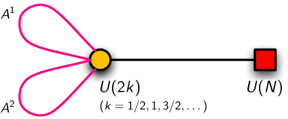
[Uncaptioned image][Uncaptioned image][Uncaptioned image][Uncaptioned image][Uncaptioned image]

2 S​U​(N)SU(N) instantons on ℂ2/ℤn\mathbb{C}^{2}/\mathbb{Z}_{n}

This section introduces the quiver and geometrical data for S​U​(N)SU(N) instantons on ℂ2/ℤn\mathbb{C}^{2}/\mathbb{Z}_{n}, following which we discuss the Molien integral as well as a localisation method for the Hilbert series computation. We mostly focus on one-instanton examples with n≤4n\leq 4. Generalisations for Hilbert series of kk S​U​(N)SU(N) instantons on ℂ2/ℤn\mathbb{C}^{2}/\mathbb{Z}_{n} (for generic kk and nn) are also presented.

2.1 Quiver and Geometrical Data

The quiver data to specify the moduli space for S​U​(N)SU(N) instantons on ℂ2/ℤn\mathbb{C}^{2}/\mathbb{Z}_{n} are presented in this subsection. As reviewed in appendix A, this information is related to the geometrical data of the instanton bundle.

Quiver data.

For S​U​(N)SU(N) instantons on ℂ2\mathbb{C}^{2}, the quiver data are given by the instanton number kk and the rank NN. In the case of S​U​(N)SU(N) instantons on ℂ2/ℤn\mathbb{C}^{2}/\mathbb{Z}_{n}, the quiver data are given as follows:

  1. 1.

    A kk-tuple analogue of the instanton number. We denote this by 𝒌=(k1,…,kn)\bm{k}=(k_{1},\ldots,k_{n}) with ki∈ℤ≥0k_{i}\in\mathbb{Z}_{\geq 0} for all i=1,…,ni=1,\ldots,n.

  2. 2.

    A nn-partition of NN. We denote this by 𝑵=(N1,…,Nn)\bm{N}=(N_{1},\ldots,N_{n}) such that

    N=N1+…+Nn,\displaystyle N=N_{1}+\ldots+N_{n}~, (1)

    with Ni∈ℤ≥0N_{i}\in\mathbb{Z}_{\geq 0} for all i=1,…,ni=1,\ldots,n.

These pieces of information are collected in a four dimensional 𝒩=2{\cal N}=2 quiver diagram, also known as the Kronheimer-Nakajima (KN) quiver [6]. The quiver diagram is depicted in Figure 1. The instanton moduli space corresponds to the Higgs branch of the quiver theory. Therefore, the instanton moduli space is uniquely specified by the vectors 𝒌\bm{k} and 𝑵\bm{N} (see e.g., [6, 10, 30, 14, 15, 39, 40]). It is known [41] that the KN quiver can also be realised from a system of D3 branes on a circle, D5 and NS5 branes. Such a configuration and relevant geometical data are reviewed in Appendix A.

Refer to caption
Figure 1: The Kronheimer-Nakajima quivers for S​U​(N)SU(N) instantons on ℂ2/ℤn\mathbb{C}^{2}/\mathbb{Z}_{n}. Each node denotes the unitary group with the labelled rank. The circular nodes denote gauge groups and the square nodes denote the flavour symmetries.

For each gauge group U⁡(ki)U(k_{i}), the one loop beta function coefficient βi\beta_{i} is given by

βi=Ni+ki−1+ki+1−2​ki,\displaystyle\beta_{i}=N_{i}+k_{i-1}+k_{i+1}-2k_{i}~, (2)

and the index ii runs from 1,…,n1,\ldots,n and is taken modulo nn. Note that βi\beta_{i} is also equal to the relative linking numbers of the (i+1)(i+1)-th and the ii-th NS5-branes, and that

∑i=1nβi=N.\displaystyle\sum_{i=1}^{n}\beta_{i}=N~. (3)
Geometrical Data.

The relation between the quiver data, namely 𝒌\bm{k} and 𝑵\bm{N}, and the geometrical data of the instanton bundle can be summarised as follows [6, 10, 30, 14, 15, 39, 40]:

  • •

    Rank of the instanton bundle is given by ∑i=1nNi=N\sum_{i=1}^{n}N_{i}=N.

  • •

    The monodromy at infinity is specified by the nn-partition of NN : 𝑵=(N1,N2,…,Nn)\bm{N}=(N_{1},N_{2},\ldots,N_{n}).

  • •

    The first Chern class of the instanton bundle is

    c1=∑i=1nβi​c1​(𝒯i),\displaystyle c_{1}=\sum_{i=1}^{n}\beta_{i}c_{1}(\mathcal{T}_{i})~, (4)

    where 𝒯i{\cal T}_{i} are the line bundles defined in (525). According to [10], c1c_{1} has a physical interpretation as a monopole charge coming from an integral of the field strength corresponding to the instanton configuration.

  • •

    The second Chern class of the instanton bundle is

    c2=∑i=1nβi​c2​(𝒯i)+1n​∑i=1nki.\displaystyle c_{2}=\sum_{i=1}^{n}\beta_{i}c_{2}(\mathcal{T}_{i})+\frac{1}{n}\,\sum_{i=1}^{n}k_{i}~. (5)

    It is possible to make a choice so that one of 𝒯1,…,𝒯n{\cal T}_{1},\ldots,{\cal T}_{n} is a trivial line bundle. Henceforth, we choose 𝒯n\mathcal{T}_{n} to be trivial, so that

    c1​(𝒯n)=c2​(𝒯n)=0.\displaystyle c_{1}(\mathcal{T}_{n})=c_{2}(\mathcal{T}_{n})=0~. (6)
  • •

    Given the vector 𝒌=(k1,…,kn)\bm{k}=(k_{1},\ldots,k_{n}), we define an instanton number as

    k=1n​∑i=1nki.k=\frac{1}{n}\sum_{i=1}^{n}k_{i}~. (7)

    We stress that this does not necessarily equal to the second Chern class c2c_{2}.

  • •

    In a special case that β1=⋯=βn−1=0\beta_{1}=\cdots=\beta_{n-1}=0, the monopole charge c1=0c_{1}=0 due to (4) and (6). We thus refer to this special case as the pure instanton configuration. As an immediate consequence, the instanton number is equal to the second Chern class of the instanton bundle.

2.2 The Hilbert series via the Molien integral

Refer to caption
Figure 2: The quiver for S​U​(N)SU(N) instantons on ℂ2/ℤ2\mathbb{C}^{2}/\mathbb{Z}_{2}: 𝒌=(k1,k2)\bm{k}=(k_{1},k_{2}), 𝑵=(N1,N2)\bm{N}=(N_{1},N_{2}) with N=N1+N2N=N_{1}+N_{2}. The square nodes represent the flavor symmetries, whereas the circular nodes represent gauge symmetries. Each line between the groups U⁡(r1)U(r_{1}) and U⁡(r2)U(r_{2}) represent r1​r2r_{1}r_{2} hypermultiplets in the bi-fundamental representation.

In this subsection, we focus on the computation of the Hilbert series with a particular emphasis on the S​U​(N)SU(N) instanton on ℂ2/ℤ2\mathbb{C}^{2}/\mathbb{Z}_{2}. The quiver data is given by 𝒌=(k1,k2)\bm{k}=(k_{1},k_{2}) and 𝑵=(N1,N2)\bm{N}=(N_{1},N_{2}) with N=N1+N2N=N_{1}+N_{2}. The Higgs branch of this theory is identified with the moduli space of the corresponding instanton.

Refer to caption
Figure 3: Quiver diagram in 4d 𝒩=1{\cal N}=1 notation for S​U​(N)SU(N) instantons on ℂ2/ℤ2\mathbb{C}^{2}/\mathbb{Z}_{2}: 𝒌=(k1,k2)\bm{k}=(k_{1},k_{2}), 𝑵=(N1,N2)\bm{N}=(N_{1},N_{2}) with N=N1+N2N=N_{1}+N_{2}. The superpotential is given by (8).
Quiver and Superpotential.

Using a similar method presented in [23, 24], we can compute the Hilbert series associated to the instanton moduli space in question. We translate the 4d 𝒩=2{\cal N}=2 quiver into 𝒩=1{\cal N}=1 language with the corresponding quiver diagram depicted in Figure 3. The 𝒩=1{\cal N}=1 superpotential is

W\displaystyle W =ϵα1​α2​[(X12α1)b1a1​(φ2)b2b1​(X21α2)a1b2−(X21α1)a1b1​(φ1)a2a1​(X12α2)b1a2]+\displaystyle=\epsilon_{\alpha_{1}\alpha_{2}}\left[(X^{\alpha_{1}}_{12})^{a_{1}}_{~b_{1}}(\varphi_{2})^{b_{1}}_{~b_{2}}(X^{\alpha_{2}}_{21})^{b_{2}}_{~a_{1}}-(X^{\alpha_{1}}_{21})^{b_{1}}_{~a_{1}}(\varphi_{1})^{a_{1}}_{~a_{2}}(X^{\alpha_{2}}_{12})^{a_{2}}_{~b_{1}}\right]+
A~a1i1​(φ1)a2a1​Ai1a2+B~b1j1​(φ2)b2b1​Bj1b2,\displaystyle\quad\widetilde{A}_{a_{1}}^{i_{1}}(\varphi_{1})_{~a_{2}}^{a_{1}}A_{i_{1}}^{a_{2}}+\widetilde{B}^{j_{1}}_{b_{1}}(\varphi_{2})_{~b_{2}}^{b_{1}}B^{b_{2}}_{j_{1}}~, (8)

where a,a1,a2,…=1,…,k1a,a_{1},a_{2},\ldots=1,\ldots,k_{1} are the indices for the gauge group U⁡(k1)U(k_{1}), b,b1,b2,…=1,…,k2b,b_{1},b_{2},\ldots=1,\ldots,k_{2} are the indices for the gauge group U⁡(k2)U(k_{2}), i,i1,i2,…=1,…,N1i,i_{1},i_{2},\ldots=1,\ldots,N_{1} are the fundamental indices for the flavor symmetry group U⁡(N1)U(N_{1}) and j,j1,j2,…=1,…,N2j,j_{1},j_{2},\ldots=1,\ldots,N_{2} are the fundamental indices for the flavor symmetry group U⁡(N2)U(N_{2}). Note that there is an S​U​(2)SU(2) global symmetry under which each of X12αX^{\alpha}_{12} and X21αX^{\alpha}_{21} transforms as a doublet, where α,α1,α2,…=1,2\alpha,\alpha_{1},\alpha_{2},\ldots=1,2 are the fundamental indices for this global symmetry which we will refer to as S​U​(2)xSU(2)_{x}.

Given that the theory has 𝒩=2\mathcal{N}=2 supersymmetry, the S​U​(2)SU(2) RR-symmetry transforms each of the following pairs of chiral fields as doublets,

{(X121(X212)†),(X122(X211)†)},(Ai1(A~i1)†)(Bj1(B~j1)†),\left\{\left(\begin{array}[]{c}X_{12}^{1}\\ (X_{21}^{2})^{\dagger}\end{array}\right),\qquad\left(\begin{array}[]{c}X_{12}^{2}\\ (X_{21}^{1})^{\dagger}\end{array}\right)\right\},\qquad\left(\begin{array}[]{c}A_{i_{1}}\\ (\widetilde{A}^{i_{1}})^{\dagger}\end{array}\right)\qquad\left(\begin{array}[]{c}B_{j_{1}}\\ (\widetilde{B}^{j_{1}})^{\dagger}\end{array}\right)~, (9)

where the pair in the curly bracket transforms as a doublet under S​U​(2)xSU(2)_{x} and the others transform as singlets under S​U​(2)xSU(2)_{x}. The scalar in each vector multiplet transforms as a singlet under S​U​(2)SU(2) RR-symmetry.

In 𝒩=1{\cal N}=1 formalism, only one generator of S​U​(2)RSU(2)_{R}, which we will call U​(1)tU(1)_{t}, is manifest.11 1 This U⁡(1)U(1) global symmetry is referred to as U​(1)JU(1)_{J} in, for example, [42]. Note that, when thinking of the theory as a 4d 𝒩=2\mathcal{N}=2 one, the R-symmetry is U​(1)r×S​U​(2)RU(1)_{r}\times SU(2)_{R}. On the Higgs branch, up to a normalization, the action of the U​(1)rU(1)_{r} and the U​(1)J∈S​U​(2)RU(1)_{J}\in SU(2)_{R} is identical, i.e. assigns the same charges to all fields in hypermultiplets. Therefore, each of the chiral fields X12αX^{\alpha}_{12}, X21αX^{\alpha}_{21}, AiA_{i}, A~i\widetilde{A}^{i}, BjB_{j}, B~j\widetilde{B}^{j}, coming from the hypermultiplets, carries charge +1+1 under U​(1)tU(1)_{t}, whereas the chiral fields φ1\varphi_{1} and φ2\varphi_{2}, coming from the vector multiplets, carries charge 00 under U​(1)tU(1)_{t}.

F-terms.

Since we are interested in the Higgs branch of this theory, the relevant FF-terms arising from differentiating the superpotential (8) with respect to the scalars in the vector multiplets, φ1\varphi_{1} and φ2\varphi_{2}, are given by

0\displaystyle 0 =(ℱ1)a2a1:=∂(φ1)a1a2W=−(X21α1)a2b1​(X12α2)b1a1​ϵα1​α2+Ai1a1​A~a2i1,\displaystyle=(\mathcal{F}_{1})^{a_{1}}_{~a_{2}}:=\partial_{(\varphi_{1})^{a_{2}}_{a_{1}}}W=-(X_{21}^{\alpha_{1}})^{b_{1}}_{~a_{2}}(X_{12}^{\alpha_{2}})^{a_{1}}_{~b_{1}}\epsilon_{\alpha_{1}\alpha_{2}}+A_{i_{1}}^{a_{1}}\widetilde{A}_{a_{2}}^{i_{1}}~,
0\displaystyle 0 =(ℱ2)b2b1:=∂(φ2)b1b2W=(X12α1)b2a1​(X21α2)a1b1​ϵα1​α2+Bj1b1​B~b2j1.\displaystyle=(\mathcal{F}_{2})^{b_{1}}_{~b_{2}}:=\partial_{(\varphi_{2})^{b_{2}}_{b_{1}}}W=(X_{12}^{\alpha_{1}})^{a_{1}}_{~b_{2}}(X_{21}^{\alpha_{2}})^{b_{1}}_{~a_{1}}\epsilon_{\alpha_{1}\alpha_{2}}+B_{j_{1}}^{b_{1}}\widetilde{B}_{b_{2}}^{j_{1}}~. (10)
Gauge and Global Symmetries.

The transformation rule of the chiral fields and the FF-terms under the gauge and global symmetries are summarised in Table 1.

U⁡(k1)U⁡(k2)U​(1)tS​U​(2)xU⁡(N1)U⁡(N2)X12α□+1□¯−11□1010X21α□¯−1□+11□1010φ1𝐀𝐝𝐣1011010φ21𝐀𝐝𝐣011010A□+11011□¯−110A~□¯−11011□+110B10□+11110□¯−1B~10□¯−11110□+1ℱ1𝐀𝐝𝐣10211010ℱ210𝐀𝐝𝐣211010\begin{array}[]{|c | c c | c c c c c |c }\hline\cr&U(k_{1})&U(k_{2})&U(1)_{t}&SU(2)_{x}&U(N_{1})&U(N_{2})&\\ \hline\cr\hline\cr X_{12}^{\alpha}&\Box_{+1}&\overline{\Box}_{-1}&1&\Box&\textbf{1}_{0}&\textbf{1}_{0}&\\ X_{21}^{\alpha}&\overline{\Box}_{-1}&\Box_{+1}&1&\Box&\textbf{1}_{0}&\textbf{1}_{0}&\\ \varphi_{1}&\mathbf{Adj}&\textbf{1}&0&\textbf{1}&\textbf{1}_{0}&\textbf{1}_{0}&\\ \varphi_{2}&\textbf{1}&\mathbf{Adj}&0&\textbf{1}&\textbf{1}_{0}&\textbf{1}_{0}&\\ A&\Box_{+1}&\textbf{1}_{0}&1&\textbf{1}&\overline{\Box}_{-1}&\textbf{1}_{0}&\\ {\widetilde{A}}&\overline{\Box}_{-1}&\textbf{1}_{0}&1&\textbf{1}&\Box_{+1}&\textbf{1}_{0}&\\ B&\textbf{1}_{0}&\Box_{+1}&1&\textbf{1}&\textbf{1}_{0}&\overline{\Box}_{-1}&\\ {\widetilde{B}}&\textbf{1}_{0}&\overline{\Box}_{-1}&1&\textbf{1}&\textbf{1}_{0}&\Box_{+1}&\\ \hline\cr\mathcal{F}_{1}&\mathbf{Adj}&\textbf{1}_{0}&2&\textbf{1}&\textbf{1}_{0}&\textbf{1}_{0}&\\ \mathcal{F}_{2}&\textbf{1}_{0}&\mathbf{Adj}&2&\textbf{1}&\textbf{1}_{0}&\textbf{1}_{0}&\\ \hline\cr\end{array}

Table 1: The transformation rule of the chiral fields and the FF-terms under the gauge and global symmetries.
Moduli Space Data.

When N1N_{1} and N2N_{2} are sufficiently large compared to k1k_{1} and k2k_{2}, the gauge symmetry is completely broken on the hypermultiplet moduli space. Upon Higgsing, k1​N1+k2​N2+2​k1​k2−k12−k22k_{1}N_{1}+k_{2}N_{2}+2k_{1}k_{2}-k_{1}^{2}-k_{2}^{2} quaternionic gauge invariant degrees of freedom remain. Hence, the quaternionic dimension of the Higgs branch is given by

dimℍ​ℳ(k1,k2)(N1,N2)=k1​(N1+k2−k1)+k2​(N2+k1−k2){\rm dim}_{\mathbb{H}}\,\mathcal{M}^{(N_{1},N_{2})}_{(k_{1},k_{2})}=k_{1}\,(N_{1}+k_{2}-k_{1})+k_{2}\,(N_{2}+k_{1}-k_{2}) (11)

2.2.1 Hilbert Series for one S​U​(N)SU(N) instanton on ℂ2/ℤ2\mathbb{C}^{2}/\mathbb{Z}_{2}: 𝒌=(1,1)\bm{k}=(1,1) and 𝑵=(0,N)\bm{N}=(0,N).

The Molien integral formula for Hilbert Series is most conveniently expressed in terms of plethystic exponential (PE) of functions. For a multi-variable function f(x1,x2,….,xn)f(x_{1},x_{2},....,x_{n}) which vanishes at the origin, this is defined as,

PE[f(x1,x2,….,xn)]=exp(∑r=1∞f(xr1,xr2,….,xrn)r)\displaystyle\mathop{\rm PE}\left[f(x_{1},x_{2},....,x_{n})\right]=\exp\left(\sum^{\infty}_{r=1}\frac{f(x^{r}_{1},x^{r}_{2},....,x^{r}_{n})}{r}\right) (12)

The inverse function to the plethystic exponential is known as plethystic logarithm (PL). Character expansion of PL of the Hilbert Series in terms of the global symmetry group is a direct way to read off generators of the chiral ring at every level including their relations. For more details, the reader is referred to the earlier body of work in [23]-[25].
In the present example, let z1z_{1} and z2z_{2} be the fugacities for the gauge symmetry U⁡(1)×U⁡(1)U(1)\times U(1). Furthermore, let xx be fugacity of the global symmetry S​U​(2)xSU(2)_{x} and (u,𝒚)(u,\bm{y}) be the fugacities of U⁡(N)=U⁡(1)×S​U​(N)U(N)=U(1)\times SU(N).

The Hilbert series is then given by the Molien integral

g(1, 1)(0,N)​(t,x,u,𝒚)=∮|z1|=1d​z1(2​π​i)​z1​∮|z2|=1d​z2(2​π​i)​z2​χB​(t,u,𝒚,z2)​χX​(t,x,z1,z2)χF​(t)\displaystyle g_{(1,\,1)}^{(0,\,N)}(t,x,u,\bm{y})=\oint_{|z_{1}|=1}\frac{\mathrm{d}z_{1}}{(2\pi i)z_{1}}\,\oint_{|z_{2}|=1}\frac{\mathrm{d}z_{2}}{(2\pi i)z_{2}}\frac{\chi_{B}(t,u,\bm{y},z_{2})\chi_{X}(t,x,z_{1},z_{2})}{\chi_{F}(t)} (13)

where the contributions from BB, XX’s and FF-terms are given respectively by

χB​(t,u,𝒚)\displaystyle\chi_{B}(t,u,\bm{y}) =PE[[0,…,0,1]𝒚​u−1​z2​t+[1,0,…, 0]𝒚​u​z2−1​t],\displaystyle=\mathop{\rm PE}\Big[[0,\ldots,0,1]_{\bm{y}}u^{-1}z_{2}t+[1,0,\ldots,\,0]_{\bm{y}}uz_{2}^{-1}t\Big]~,
χX​(t,x,z1,z2)\displaystyle\chi_{X}(t,x,z_{1},z_{2}) =PE[[1]x​(z1​z2−1+z1−1​z2)​t],\displaystyle=\mathop{\rm PE}\Big[[1]_{x}\left(z_{1}z_{2}^{-1}+z_{1}^{-1}z_{2}\right)t\Big]~,
χF​(t)\displaystyle\chi_{F}(t) =(1−t2)−2.\displaystyle=(1-t^{2})^{-2}~. (14)

The z1z_{1} integral can be easily done. Letting z2′=z2​u−1z^{\prime}_{2}=z_{2}u^{-1}, we have

g(1, 1)(0,N)​(t,x,𝒚)\displaystyle g_{(1,\,1)}^{(0,\,N)}(t,x,\bm{y}) =gℂ2/ℤ2​(t,x)​{(1−t2)​∮|z2′|=1d​z2′z2′​PE[[0,…, 1]𝒚​z2′​t+[1,…,0,0]𝒚​z2′−1​t]}\displaystyle=g_{\mathbb{C}^{2}/\mathbb{Z}_{2}}(t,x)\Big\{(1-t^{2})\,\oint_{|z_{2}^{\prime}|=1}\frac{\mathrm{d}z^{\prime}_{2}}{z^{\prime}_{2}}\,\mathop{\rm PE}\Big[[0,\ldots,\,1]_{\bm{y}}z^{\prime}_{2}t+[1,\ldots,0,0]_{\bm{y}}{z^{\prime}_{2}}^{-1}t\Big]\Big\}
=∑n1=0∞∑n2=0∞[2​n1;n2,0,…,0,n2]x,𝒚​t2​n1+2​n2\displaystyle=\sum_{n_{1}=0}^{\infty}\sum_{n_{2}=0}^{\infty}[2n_{1};n_{2},0,\dots,0,n_{2}]_{x,\bm{y}}\,\,t^{2n_{1}+2n_{2}}
=gℂ2/ℤ2​(t,x)×g~1,S​U​(N),ℂ2​(t,𝒚),\displaystyle=g_{\mathbb{C}^{2}/\mathbb{Z}_{2}}(t,x)\times\widetilde{g}_{1,SU(N),\mathbb{C}^{2}}(t,\bm{y})~, (15)

where

gℂ2/ℤ2​(t,x)\displaystyle g_{\mathbb{C}^{2}/\mathbb{Z}_{2}}(t,x) =(1−t4)​PE[[2]x​t2]=(1+t2)(1−t2​x2)​(1−t2​x−2)=∑n=0∞[2​n]x​t2​n,\displaystyle=(1-t^{4})\mathop{\rm PE}[[2]_{x}t^{2}]=\frac{(1+t^{2})}{(1-t^{2}\,x^{2})\,(1-t^{2}\,x^{-2})}=\sum_{n=0}^{\infty}[2n]_{x}t^{2n}~, (16)
g~1,S​U​(N),ℂ2​(t,𝒚)\displaystyle\widetilde{g}_{1,SU(N),\mathbb{C}^{2}}(t,\bm{y}) =∑n=0∞[n,0,…,0,n]𝒚​t2​n.\displaystyle=\sum_{n=0}^{\infty}[n,0,\ldots,0,n]_{\bm{y}}t^{2n}~. (17)

From [23], g~1,S​U​(N),ℂ2​(t,𝒃)\widetilde{g}_{1,SU(N),\mathbb{C}^{2}}(t,\bm{b}) can be identified as the Hilbert series for the reduced instanton moduli space of one S​U​(N)SU(N) instanton on ℂ2\mathbb{C}^{2}. On the other hand, gℂ2/ℤ2​(t,x)g_{\mathbb{C}^{2}/\mathbb{Z}_{2}}(t,x) is the Hilbert series for ℂ2/ℤ2\mathbb{C}^{2}/\mathbb{Z}_{2}. This infinite family of quivers therefore gives a class of instantons where the moduli space is a product of ℂ2/ℤ2\mathbb{C}^{2}/\mathbb{Z}_{2} and a reduced moduli space of instantons on ℂ2\mathbb{C}^{2}. In the next subsection, we will encounter a class of instantons where the moduli space does not factorise into such simple components as above.

The plethystic logarithm of the Hilbert series (15) is

PL[g(1, 1)(0,N)​(t,x,𝒚)]\displaystyle\mathop{\rm PL}\left[g_{(1,\,1)}^{(0,\,N)}(t,x,\bm{y})\right] =([2]𝒙​t2−t4)+[1,0,…,0,1]𝒚​t2−([0,1,0,…,0,1,0]𝒚+[1,0,…,0,1]𝒚CLOSE\displaystyle=([2]_{\bm{x}}t^{2}-t^{4})+[1,0,\ldots,0,1]_{\bm{y}}t^{2}-([0,1,0,\ldots,0,1,0]_{\bm{y}}+[1,0,\ldots,0,1]_{\bm{y}}
OPEN+[0,…,0]𝒚)​t4+….\displaystyle\qquad+[0,\ldots,0]_{\bm{y}})t^{4}+\ldots~. (18)

In order to check that the order of the pole of the function g(1, 1)(0,N)​(t,x,𝒚)g_{(1,\,1)}^{(0,\,N)}(t,x,\bm{y}) at t=1t=1 gives the correct complex dimension of the instanton moduli space, one can re-sum the series in equation (17) at 𝒚=(1,1,…..,1)\bm{y}=\left(1,1,.....,1\right). Using the dimension formula for the representations of S​U​(N)SU(N) [23], we have

dim[n,0,0,….,0,n]=((N−2+n)!n!​(N−2)!)2(2​n+N−1N−1)\displaystyle\mbox{dim}\left[n,0,0,....,0,n\right]=\left(\frac{(N-2+n)!}{n!(N-2)!}\right)^{2}\left(\frac{2n+N-1}{N-1}\right) (19)

The unrefined index for the HS will therefore be given as

g(1, 1)(0,N)​(t)\displaystyle g_{(1,\,1)}^{(0,\,N)}(t) =1+t2(1−t2)2×[∑n=0∞dim​[n,0,…,0,n]​t2​n]\displaystyle=\frac{1+t^{2}}{(1-t^{2})^{2}}\times\left[\sum_{n=0}^{\infty}\mbox{dim}[n,0,\ldots,0,n]t^{2n}\right]
=1+t2(1−t2)2×[F12​(N−1,N−1,1,t2)+2​t2​(N−1)​F12​(N,N,2,t2)]\displaystyle=\frac{1+t^{2}}{(1-t^{2})^{2}}\times\left[{}_{2}F_{1}\left(N-1,N-1,1;t^{2}\right)+2t^{2}(N-1){}_{2}F_{1}\left(N,N,2;t^{2}\right)\right] (20)

where F12​(a,b,c,x){}_{2}F_{1}\left(a,b,c;x\right) is a hypergeometric function of the indicated type.
We enumerate the unrefined HS for the first few cases of (0,N)(0,N) instantons of instanton number one:

N=1:g(1, 1)(0,N=1)​(t)=\displaystyle N=1\;\;:\;\;g_{(1,\,1)}^{(0,\,N=1)}(t)= 1+t2(1−t2)2\displaystyle\frac{1+t^{2}}{\left(1-t^{2}\right)^{2}}
N=2:g(1, 1)(0,N=2)​(t)=\displaystyle N=2\;\;:\;\;g_{(1,\,1)}^{(0,\,N=2)}(t)= (1+t2)2(1−t2)4\displaystyle\frac{\left(1+t^{2}\right)^{2}}{\left(1-t^{2}\right)^{4}}
N=3:g(1, 1)(0,N=3)​(t)=\displaystyle N=3\;\;:\;\;g_{(1,\,1)}^{(0,\,N=3)}(t)= (1+t2)​(1+4​t2+t4)(1−t2)6\displaystyle\frac{\left(1+t^{2}\right)\left(1+4t^{2}+t^{4}\right)}{\left(1-t^{2}\right)^{6}}
N=4:g(1, 1)(0,N=4)​(t)=\displaystyle N=4\;\;:\;\;g_{(1,\,1)}^{(0,\,N=4)}(t)= (1+t2)2​(1+8​t2+t4)(1−t2)8.\displaystyle\frac{\left(1+t^{2}\right)^{2}\left(1+8t^{2}+t^{4}\right)}{\left(1-t^{2}\right)^{8}}~. (21)

Note that the order of the pole at t=1t=1 in each case matches with the complex dimension of the instanton moduli space.
For a generic NN, the order of the pole can be obtained by considering the asymptotic form of the hypergeometric functions in the formula for g(1, 1)(0,N)​(t)g_{(1,\,1)}^{(0,\,N)}(t) as t→1t\to 1.

g(1, 1)(0,N)​(t→1)∼1(1−t2)2×1(1−t2)2​N−2=1(1−t2)2​N\displaystyle g_{(1,\,1)}^{(0,\,N)}(t\to 1)\sim\frac{1}{(1-t^{2})^{2}}\times\frac{1}{(1-t^{2})^{2N-2}}=\frac{1}{(1-t^{2})^{2N}} (22)

The order of the pole gives the correct complex dimension of the instanton moduli space as expected.
One can obviously unrefine the Molien integral formula directly and evaluate the residue using Leibniz’s derivative rule to obtain the following equivalent formula for the unrefined HS,

g(1, 1)(0,N)​(t)=1+t2(1−t2)2×∑n=0N−1(N−1n)2​t2​n(1−t2)2​(N−1)\displaystyle g_{(1,\,1)}^{(0,\,N)}(t)=\frac{1+t^{2}}{(1-t^{2})^{2}}\times\frac{\sum^{N-1}_{n=0}{N-1\choose n}^{2}t^{2n}}{(1-t^{2})^{2(N-1)}} (23)

The order of the t=1t=1 pole for a generic theory of the class (0,N)(0,N) can be directly read off from the above formula and matches with the moduli space dimension of the corresponding instanton, as expected.

2.2.2 Hilbert Series for one S​U​(N+1)SU(N+1) instanton on ℂ2/ℤ2\mathbb{C}^{2}/\mathbb{Z}_{2}: 𝒌=(1,1)\bm{k}=(1,1) and 𝑵=(1,N)\bm{N}=(1,N).

The Hilbert series is given by the Molien integral

g(1, 1)(1,N)​(t,x,u1,u2,𝒚)\displaystyle g_{(1,\,1)}^{(1,\,N)}(t,x,u_{1},u_{2},\bm{y})
=∮|z1|=1d​z1(2​π​i)​z1​∮|z2|=1d​z2(2​π​i)​z2​χA​(t,u1,z1)​χB​(t,u2,𝒚,z2)​χX​(t,x,z1,z2)χF​(t),\displaystyle=\oint_{|z_{1}|=1}\frac{\mathrm{d}z_{1}}{(2\pi i)z_{1}}\oint_{|z_{2}|=1}\frac{\mathrm{d}z_{2}}{(2\pi i)z_{2}}\frac{\chi_{A}(t,u_{1},z_{1})\chi_{B}(t,u_{2},\bm{y},z_{2})\chi_{X}(t,x,z_{1},z_{2})}{\chi_{F}(t)}~, (24)

where the contributions from AA, BB, XX’s and FF-terms are given respectively by

χA​(t,u1,z1)\displaystyle\chi_{A}(t,u_{1},z_{1}) =PE[u1−1​z1​t+u1​z1−1​t],\displaystyle=\mathop{\rm PE}\Big[u_{1}^{-1}z_{1}t+u_{1}z_{1}^{-1}t\Big]~,
χB​(t,u2,𝒚,z2)\displaystyle\chi_{B}(t,u_{2},\bm{y},z_{2}) =PE[[0,…,0,1]𝒚​u2−1​z2​t+[1,0,…, 0]𝒚​u2​z2−1​t],\displaystyle=\mathop{\rm PE}\Big[[0,\ldots,0,1]_{\bm{y}}u_{2}^{-1}z_{2}t+[1,0,\ldots,\,0]_{\bm{y}}u_{2}z_{2}^{-1}t\Big]~,
χX​(t,x,z1,z2)\displaystyle\chi_{X}(t,x,z_{1},z_{2}) =PE[[1]x​(z1​z2−1+z1−1​z2)​t],\displaystyle=\mathop{\rm PE}\Big[[1]_{x}\left(z_{1}z_{2}^{-1}+z_{1}^{-1}z_{2}\right)t\Big]~,
χF​(t)\displaystyle\chi_{F}(t) =(1−t2)−2.\displaystyle=(1-t^{2})^{-2}~. (25)

Example: N=1N=1

Let us consider the case for N=1N=1. We find the Hilbert series

g(1, 1)(1, 1)​(t,x,q)=P⁡(t,x,q)(1−t2x2)​(1−t2​x2)​(1−t3​qx)​(1−t3x​q)​(1−t3​x​q)​(1−t3​xq),g_{(1,\,1)}^{(1,\,1)}(t,x,q)=\frac{P(t,x,q)}{(1-\frac{t^{2}}{x^{2}})\,(1-t^{2}\,x^{2})\,(1-\frac{t^{3}\,q}{x})\,(1-\frac{t^{3}}{x\,q})\,(1-{t^{3}\,x\,q})\,(1-\frac{t^{3}\,x}{q})}~, (26)

where P⁡(t,x,q)P(t,x,q) is a polynomial

P⁡(t,x,q)\displaystyle P(t,x,q) =1+2​t2+2​t4−(x+x−1)​(q+q−1)​t5−(x2+x−2)​t6\displaystyle=1+2\,t^{2}+2\,t^{4}-(x+x^{-1})\,(q+q^{-1})\,t^{5}-(x^{2}+x^{-2})\,t^{6}
−(x+x−1)​(q+q−1)​t7+2​t8+2​t10+t12,\displaystyle\qquad-(x+x^{-1})\,(q+q^{-1})\,t^{7}+2\,t^{8}+2\,t^{10}+t^{12}~, (27)

with q=u1​u2−1q=u_{1}u_{2}^{-1}. The unrefined Hilbert series is

g(1, 1)(1, 1)​(t,1,1)=1+2​t2+2​t3+2​t4+t6(1−t)4​(1+t)2​(1+t+t2)2g_{(1,\,1)}^{(1,\,1)}(t,1,1)=\frac{1+2\,t^{2}+2\,t^{3}+2\,t^{4}+t^{6}}{(1-t)^{4}\,(1+t)^{2}\,(1+t+t^{2})^{2}} (28)

The order of the pole at t=1t=1 matches with the complex dimension of the moduli space. We will observe to be true in subsequent examples below as well.

Note that (26) is invariant under q→q−1q\rightarrow q^{-1} due to the reflection symmetry of the quiver. Even though the U​(1)qU(1)_{q} fugacities in the refined Hilbert series can be arranged into S​U​(2)SU(2) characters, there does not seem to be such an enhancement in the Lagrangian. There may be such an enhancement at infinite coupling, but the methods which are used in this paper cannot provide the answer. This is left for future investigations.

Example: N=2N=2

The HS can be expanded in terms of the characters of S​U​(2)x×S​U​(2)y×U​(1)qSU(2)_{x}\times SU(2)_{y}\times U(1)_{q} as follows:

g(1, 1)(1, 2)​(t,x,q,y)\displaystyle g_{(1,\,1)}^{(1,\,2)}(t,x,q,y) =1+t2​([2]x+[2]y+1)+t3​[1]x​[1]y​(q+q−1)+t4​([4]x+[4]y+[2]x+[2]bCLOSE\displaystyle=1+t^{2}\left(\left[2\right]_{x}+[2]_{y}+1\right)+t^{3}\left[1\right]_{x}[1]_{y}(q+q^{-1})+t^{4}(\left[4\right]_{x}+[4]_{y}+[2]_{x}+[2]_{b}
OPEN+[2]y​[2]x+1)+….\displaystyle\qquad+[2]_{y}[2]_{x}+1)+\ldots~. (29)

where q=u1​u2−1q=u_{1}u_{2}^{-1} with u1u_{1} and u2u_{2} fugacities of the U⁡(1)U(1)’s coming from each flavour node.

The plethystic logarithm of this Hilbert series is given by

PL[g(1, 1)(1, 2)​(t,x,q,y)]\displaystyle\mathop{\rm PL}[g_{(1,\,1)}^{(1,\,2)}(t,x,q,y)] =t2​([2]x+[2]y+1)+t3​[1]x​[1]y​[1]q−2​t4−….\displaystyle=t^{2}\left(\left[2\right]_{x}+[2]_{y}+1\right)+t^{3}\left[1\right]_{x}[1]_{y}\left[1\right]_{q}-2t^{4}-\ldots~. (30)

The Hilbert series can also be partially unrefined by setting q=1q=1 or u1=u2u_{1}=u_{2} and the resultant formula can be written as an S​U​(2)x×S​U​(2)ySU(2)_{x}\times SU(2)_{y} character expansion in a nice closed form as follows,

g(1, 1)(1, 2)​(t,x,1,y)\displaystyle g_{(1,\,1)}^{(1,\,2)}(t,x,1,y) =1(1−t2)∑n1,n2,n3=0∞{[2n2+n3;2n1+n3]x,yt2​n1+2​n2+3​n3\displaystyle=\frac{1}{(1-t^{2})}\sum_{n_{1},n_{2},n_{3}=0}^{\infty}\Big\{[2n_{2}+n_{3};2n_{1}+n_{3}]_{x,y}t^{2n_{1}+2n_{2}+3n_{3}}
+[2n2+n3+1;2n1+n3+1]x,yt2​n1+2​n2+3​n3+3}\displaystyle+[2n_{2}+n_{3}+1;2n_{1}+n_{3}+1]_{x,y}t^{2n_{1}+2n_{2}+3n_{3}+3}\Big\} (31)

Upon unrefining completely, we find that

g(1, 1)(1, 2)​(t,1,1,1)\displaystyle g_{(1,\,1)}^{(1,\,2)}(t,1,1,1) =1+t+4​t2+9​t3+13​t4+12​t5+13​t6+9​t7+4​t8+t9+t10(1−t)6​(1+t)4​(1+t+t2)3\displaystyle=\frac{1+t+4\,t^{2}+9\,t^{3}+13\,t^{4}+12\,t^{5}+13\,t^{6}+9\,t^{7}+4\,t^{8}+t^{9}+t^{10}}{(1-t)^{6}\,(1+t)^{4}\,(1+t+t^{2})^{3}}
=1+7​t2+8​t3+26​t4+40​t5+88​t6+120​t7+233​t8+312​t9+….\displaystyle=1+7t^{2}+8t^{3}+26t^{4}+40t^{5}+88t^{6}+120t^{7}+233t^{8}+312t^{9}+\ldots~. (32)

Example: N=3N=3

The Hilbert series can be partially unrefined by setting q=1q=1 or u1=u2u_{1}=u_{2} and the resultant formula can be written as an S​U​(2)x×S​U​(3)𝒚SU(2)_{x}\times SU(3)_{\bm{y}} character expansion:

g(1, 1)(1, 3)​(t,x,1,𝒚)\displaystyle g_{(1,\,1)}^{(1,\,3)}(t,x,1,\bm{y}) =1(1−t2)∑n1,n2,n3=0∞{[2n2+n3;n1+n3,n1]x,𝒚t2​n1+2​n2+3​n3\displaystyle=\frac{1}{(1-t^{2})}\sum_{n_{1},n_{2},n_{3}=0}^{\infty}\Big\{[2n_{2}+n_{3};n_{1}+n_{3},n_{1}]_{x,\bm{y}}t^{2n_{1}+2n_{2}+3n_{3}}
+[2n2+n3+1;n1,n1+n3+1]x,𝒚t2​n1+2​n2+3​n3+3}\displaystyle+[2n_{2}+n_{3}+1;n_{1},n_{1}+n_{3}+1]_{x,\bm{y}}t^{2n_{1}+2n_{2}+3n_{3}+3}\Big\} (33)

The corresponding unrefined Hilbert series is

g(1, 1)(1, 3)​(t,1,1,𝟏)\displaystyle g_{(1,\,1)}^{(1,\,3)}(t,1,1,\bm{1}) =1+2​t+9​t2+24​t3+50​t4+76​t5+108​t6+120​t7+108​t8+palindrome+t14(1−t)8​(1+t)6​(1+t+t2)4.\displaystyle=\frac{1+2t+9t^{2}+24t^{3}+50t^{4}+76t^{5}+108t^{6}+120t^{7}+108t^{8}+\text{palindrome}+t^{14}}{(1-t)^{8}\,(1+t)^{6}\,(1+t+t^{2})^{4}}~. (34)

The Case of General NN

One can now summarise the case of general NN. Unrefining partially by setting q=1q=1 or u1=u2u_{1}=u_{2}, the Hilbert series can be written as an S​U​(2)x×S​U​(N)ySU(2)_{x}\times SU(N)_{y} character expansion for any N>1N>1,

g(1, 1)(1,N)​(t,x,1,𝒚)\displaystyle g_{(1,\,1)}^{(1,\,N)}(t,x,1,\bm{y}) =1(1−t2)∑n1,n2,n3=0∞{[2n2+n3;n1+n3,0,…,0,n1]x,𝒚t2​n1+2​n2+3​n3\displaystyle=\frac{1}{(1-t^{2})}\sum_{n_{1},n_{2},n_{3}=0}^{\infty}\Big\{[2n_{2}+n_{3};n_{1}+n_{3},0,\dots,0,n_{1}]_{x,\bm{y}}t^{2n_{1}+2n_{2}+3n_{3}}
+[2n2+n3+1;n1,0,…,0,n1+n3+1]x,𝒚t2​n1+2​n2+3​n3+3}.\displaystyle+[2n_{2}+n_{3}+1;n_{1},0,\dots,0,n_{1}+n_{3}+1]_{x,\bm{y}}t^{2n_{1}+2n_{2}+3n_{3}+3}\Big\}~. (35)

The plethystic logarithm for the corresponding fully refined Hilbert series is

PL[g(1,1)(1,N)​(t,x,q,𝒚)]\displaystyle\mathop{\rm PL}[g^{(1,N)}_{(1,1)}(t,x;q;\bm{y})]
=([2;0,…,0]+[0;1,0,…,0,1]+[0;0,…,0])​t2+\displaystyle=([2;0,\ldots,0]+[0;1,0,\ldots,0,1]+[0;0,\ldots,0])t^{2}+
+(q−1​[1;1,0,…,0]+q⁡[1;0,…,0,1])​t3−…,\displaystyle\qquad+(q^{-1}[1;1,0,\ldots,0]+q[1;0,\ldots,0,1])t^{3}-\ldots~, (36)

where the notation [a;b1,…,bn][a;b_{1},\ldots,b_{n}] denotes the representation of the global symmetry S​U​(2)x×S​U​(N)SU(2)_{x}\times SU(N), where the fugacity q=u1​u2−1q=u_{1}u_{2}^{-1} where u1u_{1} and u2u_{2} correspond to the U⁡(1)U(1) coming from each flavour node.

The above character expansion can be used to obtain a formula for the unrefined index for a generic NN. We define a function K⁡(x,y,N)K\left(x,y,N\right) such that,

K⁡(a1,aN−1,N)=\displaystyle K\left(a_{1},a_{N-1},N\right)= dim​[a1,0,…,0,aN−1]S​U​(N)\displaystyle\mbox{dim}\left[a_{1},0,...,0,a_{N-1}\right]_{SU(N)}
=\displaystyle= (a1+aN−2+N−1)​G⁡(N−1)G⁡(N+1)​(a1+1)N−2​(aN−2+1)N−2\displaystyle(a_{1}+a_{N-2}+N-1)\frac{G(N-1)}{G(N+1)}\left(a_{1}+1\right)_{N-2}\left(a_{N-2}+1\right)_{N-2} (37)

where G⁡(z)G(z) is a Barnes GG-function and (a)n=a⁡(a−1)​(a−2)​….(a−n+1)\left(a\right)_{n}=a(a-1)(a-2)....(a-n+1) is the Pochhammer symbol.
The above formula may be directly obtained from the following dimension formula of S​U​(N)SU(N) irreps in terms of Dynkin labels [43]:

dim[a1,a2,….,aN−1]=∏1≤i<j≤N(ai+…..+aj−1)+j−ij−i\displaystyle\mbox{dim}\left[a_{1},a_{2},....,a_{N-1}\right]=\prod_{1\leq i<j\leq N}\frac{(a_{i}+.....+a_{j-1})+j-i}{j-i} (38)

One can therefore write the following formula for the unrefined HS:

g(1, 1)(1,N)​(t,1,1,𝟏)\displaystyle g_{(1,\,1)}^{(1,\,N)}(t,1,1,\bm{1}) =1(1−t2)∑n1,n2,n3=0∞{(2n2+n3+1)K(n1+n3,n1,N)t2​n1+2​n2+3​n3\displaystyle=\frac{1}{(1-t^{2})}\sum_{n_{1},n_{2},n_{3}=0}^{\infty}\Big\{\left(2n_{2}+n_{3}+1\right)K\left(n_{1}+n_{3},n_{1},N\right)t^{2n_{1}+2n_{2}+3n_{3}}
+(2n2+n3+2)K(n1,n1+n3+1,N)t2​n1+2​n2+3​n3+3}.\displaystyle+\left(2n_{2}+n_{3}+2\right)K\left(n_{1},n_{1}+n_{3}+1,N\right)t^{2n_{1}+2n_{2}+3n_{3}+3}\Big\}~. (39)

One cannot re-sum the above series to a closed form for a generic NN, but one can quickly check that the result agrees with the unrefined HS for N=2,3N=2,3. One can use it to obtain the unrefined series for the N=4N=4 case as well.

g(1, 1)(1,N=4)​(t,1,1,𝟏)\displaystyle g_{(1,\,1)}^{(1,\,N=4)}(t,1,1,\bm{1})
=(1+3​t+17​t2+54​t3+143​t4+293​t5+533​t6+798​t7+1018​t8+1088​t9+palindrome+t18)(1−t)10​(1+t)8​(1+t+t2)5\displaystyle=\frac{\left(1+3t+17t^{2}+54t^{3}+143t^{4}+293t^{5}+533t^{6}+798t^{7}+1018t^{8}+1088t^{9}+\mbox{palindrome}+t^{18}\right)}{(1-t)^{10}(1+t)^{8}\left(1+t+t^{2}\right)^{5}} (40)

with the order of the pole at t=1t=1 again matching the complex dimension of the instanton moduli space.

Note that Hilbert series for the class of S​U​(N+1)SU(N+1) instantons discussed above does not factorize into Hilbert series for the center of mass motion on ℂ2/ℤ2\mathbb{C}^{2}/\mathbb{Z}_{2} times Hilbert series of the reduced moduli space. This shows that, on the contrary to the ℂ2\mathbb{C}^{2} case in [23, 24], generically the moduli space for instantons on ALE space does not have a factorisation property.

Refer to caption
Figure 4: The 𝒩=1\mathcal{N}=1 quiver for S​U​(N)SU(N) instantons on ℂ2/ℤn\mathbb{C}^{2}/\mathbb{Z}_{n}.

One instanton in a Generic Necklace Quiver: 𝒌=(1,…,1)\bm{k}=(1,\dots,1) and 𝑵=(N1,…,Nn)\bm{N}=(N_{1},\dots,N_{n}).

The Molien integral formula for the Hilbert series can be generalised for a cyclic quiver of the form as shown in Figure 4. For n>2n>2, there is no analogue of the S​U​(2)xSU(2)_{x} global symmetry. The generalisation is for 𝒌=(1,…,1)\bm{k}=(1,\dots,1) and 𝑵=(N1,…,Nn)\bm{N}=(N_{1},\dots,N_{n}) and takes the following form,

g(1,…,1)(N1,…,Nn)​(t,𝒚j)\displaystyle g^{(N_{1},\dots,N_{n})}_{(1,\dots,1)}(t,\bm{y}_{j})
=∮|z1|=1d​z1(2​π​i)​z1​…​∮|zn|=1d​zn(2​π​i)​zn​∏j=1nχAj​(t,uj,𝒚j,zj)​χX​(t,zj)χF​(t),\displaystyle=\oint_{|z_{1}|=1}\frac{\mathrm{d}z_{1}}{(2\pi i)z_{1}}\dots\oint_{|z_{n}|=1}\frac{\mathrm{d}z_{n}}{(2\pi i)z_{n}}\frac{\prod_{j=1}^{n}\chi_{A_{j}}(t,u_{j},\bm{y}_{j},z_{j})~\chi_{X}(t,z_{j})}{\chi_{F}(t)}~~, (41)

where the contributions from AjA_{j} (with j=1,…,nj=1,\ldots,n) , XX’s and FF-terms are given by

χAj​(t,uj,𝒚j,zj)\displaystyle\chi_{A_{j}}(t,u_{j},\bm{y}_{j},z_{j}) =PE[[0,…,0,1]𝒚j​uj−1​zj​t+[1,0,…,0]𝒚j​uj​zj−1​t],\displaystyle=\mathop{\rm PE}\Big[[0,\dots,0,1]_{\bm{y}_{j}}u_{j}^{-1}z_{j}t+[1,0,\dots,0]_{\bm{y}_{j}}u_{j}z_{j}^{-1}t\Big]~~,
χX​(t,zj)\displaystyle\chi_{X}(t,z_{j}) =PE[∑j=1n(zj−1​zj+1​t+zj+1−1​zj​t)],\displaystyle=\mathop{\rm PE}\Big[\sum_{j=1}^{n}(z_{j}^{-1}z_{j+1}t+z_{j+1}^{-1}z_{j}t)\Big]~~,
χF​(t)\displaystyle\chi_{F}(t) =(1−t2)−n,\displaystyle=(1-t^{2})^{-n}~~, (42)

where [1,0,…,0]𝒚j[1,0,\dots,0]_{\bm{y}_{j}} and [0,…,0,1]𝒚j[0,\dots,0,1]_{\bm{y}_{j}} are characters of the global symmetry S​U​(Nj)SU(N_{j}).

We discuss the generators of the chiral ring of operators associated to the moduli spaces of instantons presented above and the relations connecting them in 2.4, using the Plethystic Logarithm (PL) analysis.

2.3 The Hilbert series via localisation

The Hilbert series can be computed using the Molien integral formula as in the preceding section. However, larger the rank of the gauge group, greater is computational power required to compute the multi-contour integrations corresponding to Haar measures of the gauge groups. Nevertheless, the poles and their residues can be arranged combinatorially so that the problem becomes that of an enumeration of restricted coloured partitions. In this way, the Hilbert series can be computed more efficiently. The computation of the Hilbert series from the contributions from such restricted coloured partitions is referred to as the “localisation method”. This method was applied in [30, 31, 32] (see also [34, 35]) to compute the Nekrasov partition functions for S​U​(N)SU(N) instantons on ℂ2/ℤn\mathbb{C}^{2}/\mathbb{Z}_{n}. In this section, we adapt the above technique to compute the Hilbert series.

2.3.1 The Hilbert series of kk S​U​(N)SU(N) instantons on ℂ2\mathbb{C}^{2} via localisation

Let us start out by summarising the localisation method for the Hilbert series of S​U​(N)SU(N) instantons on ℂ2\mathbb{C}^{2}. This will turn out to be very useful for the subsequent computation for ℂ2/ℤn\mathbb{C}^{2}/\mathbb{Z}_{n}. Here we follow the prescription given in Theorem 2.11 and Proposition 4.1 of [22]. The idea is also similar to Section 3.5 of [26].

Let t1,t2t_{1},t_{2} be the fugacities correspond to the U⁡(2)U(2) isometry of the space ℂ2\mathbb{C}^{2}. It is sometimes convenient to rewrite these as

t1=t​x,t2=t​x−1,\displaystyle t_{1}=tx~,\qquad t_{2}=tx^{-1}~, (43)

where tt is the fugacity of the U⁡(1)U(1) subgroup of U⁡(2)U(2), and xx is the fugacity of the S​U​(2)SU(2) subgroup. Let e1,…,eNe_{1},\ldots,e_{N} be the fugacities corresponding to the internal symmetry S​U​(N)SU(N) of instantons such that e1+…+eNe_{1}+\ldots+e_{N} is the character of the fundamental representation of S​U​(N)SU(N) and

∏α=1Neα=1.\displaystyle\prod_{\alpha=1}^{N}e_{\alpha}=1~. (44)

Localization fixes the gauge field configuration such that the instantons are located at the origin. Such fixed instantons are labelled by an NN-tuple of Young diagrams, denoted by 𝒀=(Y1,Y2,…,YN)\bm{Y}=(Y_{1},Y_{2},\ldots,Y_{N}). We refer to each element by YαY_{\alpha}, with α=1,…,N\alpha=1,\ldots,N, and we allow the cases in which there exist empty diagrams. The instanton number kk is given by the total number of boxes

k=|𝒀|:=∑α=1N|Yα|.\displaystyle k=|\bm{Y}|:=\sum_{\alpha=1}^{N}|Y_{\alpha}|~. (45)

Let us define

Nα,β𝒀​(t1,t2,𝒆)\displaystyle N_{\alpha,\beta}^{\bm{Y}}(t_{1},t_{2},\bm{e}) =∑s∈Yα(eαeβ​t1−lYβ​(s)​t21+aYα​(s)+eβeα​t11+lYβ​(s)​t2−aYα​(s)),\displaystyle=\sum_{s\in Y_{\alpha}}\left(\frac{e_{\alpha}}{e_{\beta}}t_{1}^{-l_{Y_{\beta}}(s)}t_{2}^{1+a_{Y_{\alpha}}(s)}+\frac{e_{\beta}}{e_{\alpha}}t_{1}^{1+l_{Y_{\beta}}(s)}t_{2}^{-a_{Y_{\alpha}}(s)}\right)~, (46)

where for a given box ss at the aa-th column and bb-th row, i.e.  at the coordinates (a,b)(a,b), of a given Young diagram Y=(λ1≥λ2≥…)Y=(\lambda_{1}\geq\lambda_{2}\geq\ldots), one can define aY​(s)a_{Y}(s) and lY​(s)l_{Y}(s), known as the arm length and the leg length, as follows:

aY​(s)=λa−b,lY​(s)=λb′−a,\displaystyle a_{Y}(s)=\lambda_{a}-b~,\qquad l_{Y}(s)=\lambda^{\prime}_{b}-a~, (47)

where λb′\lambda^{\prime}_{b} corresponds to the transpose diagram of YY, namely YT=(λ1′≥λ2′≥…)Y^{T}=(\lambda^{\prime}_{1}\geq\lambda^{\prime}_{2}\geq\ldots). Note that in (46), if s∈Yαs\in Y_{\alpha} but s∉Yβs\notin Y_{\beta}, then lYβ​(s)l_{Y_{\beta}}(s) is negative.

The Hilbert series of kk S​U​(N)SU(N) instantons on ℂ2\mathbb{C}^{2} is then given by

Hk,ℂ2N(t1,t2,𝒆)=∑𝒀:|𝒀|=kPE[∑α,β=1NNα,β𝒀(t1,t2,𝒆)],\displaystyle H^{N}_{k,\mathbb{C}^{2}}(t_{1},t_{2},\bm{e})=\sum_{\bm{Y}:|\bm{Y}|=k}\mathop{\rm PE}\left[\sum_{\alpha,\beta=1}^{N}N_{\alpha,\beta}^{\bm{Y}}(t_{1},t_{2},\bm{e})\right]~, (48)

where the summation outside the PE\mathop{\rm PE} runs over all possible NN-tuples of the Young diagrams whose total number of boxes equal to the instanton number kk. Explicit computations can be found, for example, in (4.3) of [22] and Section 3.1 of [24].

2.3.2 The Hilbert series of S​U​(N)SU(N) instantons on ℂ2/ℤn\mathbb{C}^{2}/\mathbb{Z}_{n} via localisation

In this section, we turn to S​U​(N)SU(N) instantons on ℂ2/ℤn\mathbb{C}^{2}/\mathbb{Z}_{n} and use the quiver data as stated in Section 2.1. The ℤn\mathbb{Z}_{n} orbifold acts on the fugacities t1t_{1}, t2t_{2} and eαe_{\alpha} (with α=1,…,N\alpha=1,\ldots,N) as follows. Let ω=exp⁡(2​π​i/n)\omega=\exp(2\pi i/n), the actions are

t1→ω​t1,t2→ω−1​t2,eα→ωrα​eα,\displaystyle t_{1}\rightarrow\omega t_{1}~,\qquad t_{2}\rightarrow\omega^{-1}t_{2}~,\qquad e_{\alpha}\rightarrow\omega^{r_{\alpha}}e_{\alpha}~, (49)

where rαr_{\alpha} (with 0≤rα≤n−10\leq r_{\alpha}\leq n-1) are related to the monodromy 𝑵=(N1,…,Nn)\bm{N}=(N_{1},\ldots,N_{n}) as follows:

Ni=∑α=1Nδrα,i⁡(mod​n),\displaystyle N_{i}=\sum_{\alpha=1}^{N}\delta_{r_{\alpha},i~(\mathrm{mod}~n)}~, (50)

where i⁡(mod​n)i~(\mathrm{mod}~n) runs over 0,…,n−10,\ldots,n-1. Therefore, NiN_{i} is the number of times that i⁡(mod​n)i~(\mathrm{mod}~n) appears in the vector 𝒓=(r1,…,rN)\bm{r}=(r_{1},\ldots,r_{N}). In order that the orbifold action is compatible with the S​U​(N)SU(N) symmetry, we need to impose that

∑α=1Nrα=0​(mod​n).\displaystyle\sum_{\alpha=1}^{N}r_{\alpha}=0~(\mathrm{mod}~n)~. (51)

Let us now describe the method to compute the Hilbert series of instantons on ℂ2/ℤn\mathbb{C}^{2}/\mathbb{Z}_{n} for given 𝒌\bm{k} and 𝒓\bm{r} (or 𝑵\bm{N}).

The algorithm.

Let us define a quantity as analogous to (46):

N~α,β𝒀,𝒓​(t1,t2,𝒆)\displaystyle\widetilde{N}_{\alpha,\beta}^{\bm{Y},\bm{r}}(t_{1},t_{2},\bm{e})
=∑s∈Yα(eαeβ​t1−lYβ​(s)​t21+aYα​(s)+eβeα​t11+lYβ​(s)​t2−aYα​(s))​δaYα​(s)+lYβ​(s)+1−rα+rβ​(mod​n),\displaystyle=\sum_{s\in Y_{\alpha}}\left(\frac{e_{\alpha}}{e_{\beta}}t_{1}^{-l_{Y_{\beta}}(s)}t_{2}^{1+a_{Y_{\alpha}}(s)}+\frac{e_{\beta}}{e_{\alpha}}t_{1}^{1+l_{Y_{\beta}}(s)}t_{2}^{-a_{Y_{\alpha}}(s)}\right)\delta_{a_{Y_{\alpha}}(s)+l_{Y_{\beta}}(s)+1-r_{\alpha}+r_{\beta}~(\mathrm{mod}~n)}~, (52)

Let us comment on this formula:

  • •

    The quantity in the round brackets is the same as that of instantons on ℂ2\mathbb{C}^{2}, see (46).

  • •

    The delta symbol selects only the terms in the summation that carry charge zero modulo nn, with respect to the charge assignment (49). Other terms carrying non-zero charge (modulo nn) do not contribute to the Hilbert series and are thrown away.

In addition to the above restriction, one needs to select only certain NN-tuples of Young diagrams in the summation of (48). In particular, the required Hilbert series is

H𝒌𝑵​(t1,t2,𝒆)=∑𝒀∈ℛPE[∑α,β=1NN~α,β𝒀,𝒓^​(t1,t2,𝒆)],\displaystyle H^{\bm{N}}_{\bm{k}}(t_{1},t_{2},\bm{e})=\sum_{\begin{subarray}{c}\bm{Y}\in{\cal R}\end{subarray}}\mathop{\rm PE}\left[\sum_{\alpha,\beta=1}^{N}\widetilde{N}_{\alpha,\beta}^{\bm{Y},\hat{\bm{r}}}(t_{1},t_{2},\bm{e})\right]~, (53)

where 𝒓^\hat{\bm{r}} denotes a solution (r1,…,rN)(r_{1},\ldots,r_{N}) of (50) for a given (N1,…,Nn)(N_{1},\ldots,N_{n}), and ℛ{\cal R} is a set of NN-tuples of Young diagrams such that all of the following conditions are satisfied:

  1. 1.

    The total number of boxes in 𝒀\bm{Y} is given by |𝒀|:=∑α=1NYα=∑i=1nki|\bm{Y}|:=\sum_{\alpha=1}^{N}Y_{\alpha}=\sum_{i=1}^{n}k_{i}.

  2. 2.

    Upon assigning the numbers r^α+a−b⁡(mod​n)\hat{r}_{\alpha}+a-b~(\mathrm{mod}~n) to all (a,b)(a,b) boxes of every non-trivial Young diagram Yα≠∅Y_{\alpha}\neq\emptyset for all α=1,…,N\alpha=1,\ldots,N, there must be precisely kjk_{j} boxes in total that are labelled by the number j⁡(mod​n)j~(\mathrm{mod}~n) for all j=1,…,nj=1,\ldots,n.

Notation.

It is conventional to make the following change of variables

t1=t​x,t2=t​x−1,\displaystyle t_{1}=tx~,\quad t_{2}=tx^{-1}~,
e1=y1,e2=y2y1−1,…,eN−1=yN−1yN−2−1,eN=yN−1−1,\displaystyle e_{1}=y_{1}~,\quad e_{2}=y_{2}y_{1}^{-1}~,\ldots,~e_{N-1}=y_{N-1}y_{N-2}^{-1}~,\quad e_{N}=y_{N-1}^{-1}~, (54)

Let us denote

g𝒌𝑵​(t,x,𝒚):=H𝒌𝑵​(t1,t2,𝒆)\displaystyle g^{\bm{N}}_{\bm{k}}(t,x,\bm{y}):=H^{\bm{N}}_{\bm{k}}(t_{1},t_{2},\bm{e}) (55)

written in these new variables.

Nekrasov partition function.

We mention in passing that the 4​d4d Nekrasov partititon function 𝒵𝒌𝑵​(ϵ1,ϵ2,a1,…,aN){\cal Z}^{\bm{N}}_{\bm{k}}(\epsilon_{1},\epsilon_{2},a_{1},\ldots,a_{N}) for a given 𝒌\bm{k} and 𝑵\bm{N} can be computed from the Hilbert series g𝒌𝑵​(t,x,y1,…,yN)g^{\bm{N}}_{\bm{k}}(t,x,y_{1},\ldots,y_{N}) by setting

t=e−12​β​(ϵ1+ϵ2),x=e−12​β​(ϵ1−ϵ2),yi=e−β​ai,\displaystyle t=e^{-\frac{1}{2}\beta(\epsilon_{1}+\epsilon_{2})},\quad x=e^{-\frac{1}{2}\beta(\epsilon_{1}-\epsilon_{2})},\quad y_{i}=e^{-\beta a_{i}}~, (56)

and taking the following limit [26, 22, 27, 28]:

𝒵𝒌𝑵​(ϵ1,ϵ2,a1,…,aN)=limβ→0β2​k​N​g𝒌𝑵​(t,x,y1,…,yN).\displaystyle{\cal Z}^{\bm{N}}_{\bm{k}}(\epsilon_{1},\epsilon_{2},a_{1},\ldots,a_{N})=\lim_{\beta\rightarrow 0}\beta^{2kN}g^{\bm{N}}_{\bm{k}}(t,x,y_{1},\ldots,y_{N})~. (57)

This is indeed a computation of the volume of the base of the hyperKähler cone corresponding to the instanton moduli space [44]. In Section 2.5.4, we compute explicitly the Nekrasov partition function for a given instanton number kk and compare the results with those in [45].

2.4 Generators of the moduli space

Plethystic logarithm.

The plethystic logarithm of the Hilbert series for instantons on ℂ2/ℤn\mathbb{C}^{2}/\mathbb{Z}_{n} given 𝒌\bm{k} and 𝑵\bm{N} (see Figure 1 and Figure 4) has the general form

PL[g𝒌𝑵​(t,x,𝝃1,…,𝝃n)]=(∑1≤i≤nNi≠0𝐟𝐮𝐧𝐝⁡(𝝃i)​𝐟𝐮𝐧𝐝​(𝝃i−1)⏟𝐀𝐝𝐣⁡(𝝃i))​t2+(xn+x−n)​tn\displaystyle\mathop{\rm PL}[g^{\bm{N}}_{\bm{k}}(t,x;{\bm{\xi}}_{1},\ldots,{\bm{\xi}}_{n})]=\left(\sum_{\begin{subarray}{c}1\leq i\leq n\\ N_{i}\neq 0\end{subarray}}\underbrace{{\bf fund}(\bm{\xi}_{i}){\bf fund}(\bm{\xi}_{i}^{-1})}_{{\bf Adj}(\bm{\xi}_{i})}\right)t^{2}+(x^{n}+x^{-n})t^{n}
+∑ℓ=1n−1∑1≤i≤nNi≠0(xℓ𝐟𝐮𝐧𝐝(𝝃i)𝐟𝐮𝐧𝐝(𝝃ℓ+i−1)+x−ℓ𝐟𝐮𝐧𝐝(𝝃i−1)𝐟𝐮𝐧𝐝(𝝃ℓ+i))tℓ+2\displaystyle\qquad+\sum_{\ell=1}^{n-1}\sum_{\begin{subarray}{c}1\leq i\leq n\\ N_{i}\neq 0\end{subarray}}\Big(x^{\ell}{\bf fund}({\bm{\xi}}_{i}){\bf fund}({\bm{\xi}}_{\ell+i}^{-1})+x^{-\ell}{\bf fund}({\bm{\xi}}_{i}^{-1}){\bf fund}({\bm{\xi}}_{\ell+i})\Big)t^{\ell+2}
−terms corresponding to relations from t4 onwards.\displaystyle\qquad-\text{terms corresponding to relations from $t^{4}$ onwards}~. (58)

where 𝝃1,…,𝝃n\bm{\xi}_{1},\ldots,\bm{\xi}_{n} are the global fugacities for U⁡(N1)U(N_{1}), U⁡(N2)U(N_{2}), …\ldots, U⁡(Nn)U(N_{n}) and xx is a fugacity which measures clockwise-anticlockwise fields in the cyclic quiver (see more explanation below). The index ℓ+i\ell+i is taken modulo nn and it takes values 1,2,…,n1,2,\ldots,n. Since the symmetry of the Higgs branch of the theory is S⁡(∏α=1nU⁡(Nα))S(\prod_{\alpha=1}^{n}U(N_{\alpha})), we impose the condition

∏α=1n∏i=1Nαξα,i=1.\displaystyle\prod_{\alpha=1}^{n}\prod_{i=1}^{N_{\alpha}}\xi_{\alpha,i}=1~. (59)

Note from (58) that the total number of generators is

∑i=1nNi2+2+2​∑1≤i<j≤nNi​Nj=2​N2−∑i=1nNi2+2.\displaystyle\sum_{i=1}^{n}N_{i}^{2}+2+2\sum_{1\leq i<j\leq n}N_{i}N_{j}=2N^{2}-\sum_{i=1}^{n}N_{i}^{2}+2~. (60)
Generators.

The generators of the moduli space for 𝒌=(k1,…,kn)\bm{k}=(k_{1},\ldots,k_{n}) and 𝑵=(N1,…​Nn)\bm{N}=(N_{1},\ldots N_{n}) can be read off from (58) as follows:

  1. 1.

    At order 2, there are generators in the adjoint representation of U⁡(Ni)U(N_{i}) for each i=1,…,ni=1,\ldots,n with Ni≠0N_{i}\neq 0. For each of these ii, these generators arise as gauge invariant combinations (“mesons”) of the chiral fields between the node U⁡(ki)U(k_{i}) and U⁡(Ni)U(N_{i}).

  2. 2.

    At order nn, there are two generators coming from ℂ2/ℤn\mathbb{C}^{2}/\mathbb{Z}_{n}.22 2 In fact, the space ℂ2/ℤn\mathbb{C}^{2}/\mathbb{Z}_{n} has 3 generators: one, denoted by G1G_{1}, at order 2 and two, denoted by G2,G3G_{2},G_{3}, at order nn; they are subject to the relation G1n=G2​G3G_{1}^{n}=G_{2}G_{3} at order 2​n2n. The generators G2G_{2} and G3G_{3} corresponds to the ones appearing at order tnt^{n} in (58). On the other hand, the generator G1G_{1} can be traded (using the FF term condition) with one generator at order t2t^{2} that is a singlet under S​U​(N)SU(N). These arise as gauge invariant combinations of the chiral fields in the cyclic quiver from any node U⁡(ki)U(k_{i}) back to itself in clockwise and anti-clockwise directions.

  3. 3.

    At order ℓ+2\ell+2, with ℓ=1,…,n−1\ell=1,\ldots,n-1, there are two sets of generators: one in the representation (□+1;□¯−1)(\Box_{+1};\overline{\Box}_{-1}) of U⁡(Ni)×U⁡(Nℓ+i)U(N_{i})\times U(N_{\ell+i}) and the other in (□¯−1;□+1)(\overline{\Box}_{-1};\Box_{+1}) of U⁡(Ni)×U⁡(Nℓ+i)U(N_{i})\times U(N_{\ell+i}), where i=1,…,ni=1,\ldots,n and ℓ+i\ell+i is taken modulo nn. These arise as gauge invariant combinations of the chiral fields going from the node U⁡(Ni)U(N_{i}) to a different node U⁡(Nℓ+i)U(N_{\ell+i}) and back, via ℓ\ell edges in the cyclic quiver.

Note that, in case of ℂ2/ℤ2\mathbb{C}^{2}/\mathbb{Z}_{2}, one can rewrite (58) in such a way that the S​U​(2)xSU(2)_{x} isometry is manifest, see e.g., (36).

2.5 Special case of pure instantons: 𝜷=(0,…,0,N)\bm{\beta}=(0,\ldots,0,N)

Let us consider the case of pure instantons, namly those with β1=β2=…=βn−1=0\beta_{1}=\beta_{2}=\ldots=\beta_{n-1}=0.33 3 The simplest such case is that of rank zero instantons, which we consider in appendix B. Interestingly, this case can also be studied from a holographic perspective. Given 𝜷=(0,…,0,N)\bm{\beta}=(0,\ldots,0,N), the components of 𝒌\bm{k} cannot take arbitrary values, but are constrained by (2). In the special case we are considering, (2) can be rewritten as

ki=m+∑j=1nCi​jNj,with∑j=1nCi​jNj∈ℤfor alli=1,…,n,\displaystyle k_{i}=m+\sum_{j=1}^{n}C_{ij}N_{j}~,\quad\text{with}~\sum_{j=1}^{n}C_{ij}N_{j}\in\mathbb{Z}~\text{for all}~i=1,\ldots,n~, (61)

where m=0,1,2,…m=0,1,2,\ldots and CC is the (augmented) inverse Cartan matrix of An−1A_{n-1},

Ci1​i2=min⁡(i1,i2)−i1​i2n,1≤i1,i2≤n.\displaystyle C_{i_{1}i_{2}}=\min(i_{1},i_{2})-\frac{i_{1}i_{2}}{n}~,\qquad 1\leq i_{1},i_{2}\leq n~. (62)

Below we present examples in which all possible 𝒌\bm{k} and 𝑵\bm{N} are listed, given (N,n)(N,n). One of the easiest ways to enumerate all possibilities is to start from all possible 𝒓\bm{r} subject to the contraint (51).

Examples for S​U​(2)SU(2) pure instantons

For (N,n)=(2,2)(N,n)=(2,2), i.e.  S​U​(2)SU(2) pure instantons on ℂ2/ℤ2\mathbb{C}^{2}/\mathbb{Z}_{2}, the possibilities are

𝒓=(0,0)⇒𝑵=(0,2)⇒𝒌=(m,m)⇒k=m,𝒓=(1,1)⇒𝑵=(2,0)⇒𝒌=(m+1,m)⇒k=m+12.\displaystyle\begin{array}[]{llll}\bm{r}=(0,0)&\Rightarrow\quad\bm{N}=(0,2)&\Rightarrow\quad\bm{k}=(m,m)&\Rightarrow\qquad k=m~,\\ \bm{r}=(1,1)&\Rightarrow\quad\bm{N}=(2,0)&\Rightarrow\quad\bm{k}=(m+1,m)&\Rightarrow\qquad k=m+\frac{1}{2}~.\end{array}

For (N,n)=(2,3)(N,n)=(2,3), i.e.  S​U​(2)SU(2) pure instantons on ℂ2/ℤ3\mathbb{C}^{2}/\mathbb{Z}_{3}, the possibilities are

𝒓=(0,0)⇒𝑵=(0,0,2)⇒𝒌=(m,m,m)⇒k=m,𝒓=(1,2)​or​(2,1)⇒𝑵=(1,1,0)⇒𝒌=(m+1,m+1,m)⇒k=m+23.\displaystyle\begin{array}[]{llll}\bm{r}=(0,0)&\Rightarrow\quad\bm{N}=(0,0,2)&\Rightarrow\quad\bm{k}=(m,m,m)&\Rightarrow\qquad k=m~,\\ \bm{r}=(1,2)~\text{or}~(2,1)&\Rightarrow\quad\bm{N}=(1,1,0)&\Rightarrow\quad\bm{k}=(m+1,m+1,m)&\Rightarrow\qquad k=m+\frac{2}{3}~.\end{array}

For (N,n)=(2,4)(N,n)=(2,4), i.e.  S​U​(2)SU(2) pure instantons on ℂ2/ℤ4\mathbb{C}^{2}/\mathbb{Z}_{4}, the possibilities are

𝒓=(0,0)⇒𝑵=(0,0,0,2)⇒𝒌=(m,m,m,m)⇒k=m,𝒓=(1,3)​or​(3,1)⇒𝑵=(1,0,1,0)⇒𝒌=(m+1,m+1,m+1,m)⇒k=m+34,𝒓=(2,2)⇒𝑵=(0,2,0,0)⇒𝒌=(m+1,m+2,m+1,m)⇒k=m+1.\displaystyle\begin{array}[]{llll}\bm{r}=(0,0)&\Rightarrow\quad\bm{N}=(0,0,0,2)&\Rightarrow\quad\bm{k}=(m,m,m,m)&\Rightarrow\qquad k=m~,\\ \bm{r}=(1,3)~\text{or}~(3,1)&\Rightarrow\quad\bm{N}=(1,0,1,0)&\Rightarrow\quad\bm{k}=(m+1,m+1,m+1,m)&\Rightarrow\qquad k=m+\frac{3}{4}~,\\ \bm{r}=(2,2)&\Rightarrow\quad\bm{N}=(0,2,0,0)&\Rightarrow\quad\bm{k}=(m+1,m+2,m+1,m)&\Rightarrow\qquad k=m+1~.\end{array}

Examples for S​U​(3)SU(3) pure instantons

For (N,n)=(3,2)(N,n)=(3,2), i.e.  S​U​(3)SU(3) pure instantons on ℂ2/ℤ2\mathbb{C}^{2}/\mathbb{Z}_{2}, the possibilities are

𝒓=(0,0,0)⇒𝑵=(0,3)⇒𝒌=(m,m)⇒k=m,𝒓=(0,1,1)​or perms⇒𝑵=(2,1)⇒𝒌=(m+1,m)⇒k=m+12.\displaystyle\begin{array}[]{llll}\bm{r}=(0,0,0)&\Rightarrow\quad\bm{N}=(0,3)&\Rightarrow\quad\bm{k}=(m,m)&\Rightarrow\qquad k=m~,\\ \bm{r}=(0,1,1)~\text{or perms}&\Rightarrow\quad\bm{N}=(2,1)&\Rightarrow\quad\bm{k}=(m+1,m)&\Rightarrow\qquad k=m+\frac{1}{2}~.\end{array}

For (N,n)=(3,3)(N,n)=(3,3), i.e.  S​U​(3)SU(3) pure instantons on ℂ2/ℤ3\mathbb{C}^{2}/\mathbb{Z}_{3}, the possibilities are

𝒓=(0,0,0)⇒𝑵=(0,0,3)⇒𝒌=(m,m,m)⇒k=m,𝒓=(0,1,2)​or perms⇒𝑵=(1,1,1)⇒𝒌=(m+1,m+1,m)⇒k=m+23,𝒓=(1,1,1)⇒𝑵=(3,0,0)⇒𝒌=(m+2,m+1,m)⇒k=m+1.\displaystyle\begin{array}[]{llll}\bm{r}=(0,0,0)&\Rightarrow\quad\bm{N}=(0,0,3)&\Rightarrow\quad\bm{k}=(m,m,m)&\Rightarrow\qquad k=m~,\\ \bm{r}=(0,1,2)~\text{or perms}&\Rightarrow\quad\bm{N}=(1,1,1)&\Rightarrow\quad\bm{k}=(m+1,m+1,m)&\Rightarrow\qquad k=m+\frac{2}{3}~,\\ \bm{r}=(1,1,1)&\Rightarrow\quad\bm{N}=(3,0,0)&\Rightarrow\quad\bm{k}=(m+2,m+1,m)&\Rightarrow\qquad k=m+1~.\end{array}

Examples for S​U​(4)SU(4) pure instantons

For (N,n)=(4,2)(N,n)=(4,2), i.e.  S​U​(4)SU(4) pure instantons on ℂ2/ℤ2\mathbb{C}^{2}/\mathbb{Z}_{2}, the possibilities are

𝒓=(0,0,0,0)⇒𝑵=(0,4)⇒𝒌=(m,m)⇒k=m,𝒓=(0,0,1,1)​or perms⇒𝑵=(2,2)⇒𝒌=(m+1,m)⇒k=m+12,𝒓=(1,1,1,1)⇒𝑵=(4,0)⇒𝒌=(m+2,m)⇒k=m+1.\displaystyle\begin{array}[]{llll}\bm{r}=(0,0,0,0)&\Rightarrow\quad\bm{N}=(0,4)&\Rightarrow\quad\bm{k}=(m,m)&\Rightarrow\qquad k=m~,\\ \bm{r}=(0,0,1,1)~\text{or perms}&\Rightarrow\quad\bm{N}=(2,2)&\Rightarrow\quad\bm{k}=(m+1,m)&\Rightarrow\qquad k=m+\frac{1}{2}~,\\ \bm{r}=(1,1,1,1)&\Rightarrow\quad\bm{N}=(4,0)&\Rightarrow\quad\bm{k}=(m+2,m)&\Rightarrow\qquad k=m+1~.\end{array}

2.5.1 Certain features of the moduli space of pure instantons

Subsequently, we provide several examples, including explicit Hilbert series for the pure instantons. Recall that the Kronheimer–Nakajima constructions for pure S​U​(N)SU(N) instantons correspond to 𝜷=(0,…,0,N)\bm{\beta}=(0,\ldots,0,N).

There are important features that can be drawn from these examples:

  1. 1.

    The moduli space of (n−1)/n(n-1)/n pure S​U​(N)SU(N) instantons on ℂ2/ℤn\mathbb{C}^{2}/\mathbb{Z}_{n}, corresponding to 𝒌=(1,…,1,0)\bm{k}=(1,\ldots,1,0), is ℂ2/ℤn\mathbb{C}^{2}/\mathbb{Z}_{n}.

  2. 2.

    The moduli space of one S​U​(N)SU(N) pure instanton on ℂ2/ℤn\mathbb{C}^{2}/\mathbb{Z}_{n}, corresponding to 𝒌=(1,…,1)\bm{k}=(1,\ldots,1), is

    ℂ2/ℤn×ℳ~1,S​U​(N),ℂ2,\displaystyle\mathbb{C}^{2}/\mathbb{Z}_{n}\times\widetilde{{\cal M}}_{1,SU(N),\mathbb{C}^{2}}~, (78)

    where ℳ~1,S​U​(N),ℂ2\widetilde{{\cal M}}_{1,SU(N),\mathbb{C}^{2}} is the reduced moduli space of 11 S​U​(N)SU(N) instanton on ℂ2\mathbb{C}^{2}.

We demonstrate these claims in several examples below.

2.5.2 S​U​(4)SU(4) instantons on ℂ2/ℤ2\mathbb{C}^{2}/\mathbb{Z}_{2} with 𝜷=(0,4)\bm{\beta}=(0,4)

k=1k=1

Given k=1k=1, from (2.5) there are two options in this case.

The first option.

Consider 𝒌=(1,1)\bm{k}=(1,1) and 𝑵=(0,4)\bm{N}=(0,4); we choose 𝒓=(0,0,1,1)\bm{r}=(0,0,1,1). The Hilbert series is

g(1,1)(0,4)​(t,x,𝒚)=∑m2,n2≥0[2​m2;n2,0,n2]​t2​m2+2​n2.\displaystyle g^{(0,4)}_{(1,1)}(t,x,\bm{y})=\sum_{m_{2},n_{2}\geq 0}[2m_{2};n_{2},0,n_{2}]t^{2m_{2}+2n_{2}}~. (79)

The moduli space is therefore

ℳ(1,1)(0,4)=(ℂ2/ℤ2)×ℳ~1,S​U​(4),ℂ2.\displaystyle{\cal M}^{(0,4)}_{(1,1)}=(\mathbb{C}^{2}/\mathbb{Z}_{2})\times\widetilde{{\cal M}}_{1,SU(4),\mathbb{C}^{2}}~. (80)

The unrefined Hilbert series is

g(1,1)(0,4)(t,x,{yi=1})=(1+t2)2​(1+8​t2+t4)(1−t2)8.\displaystyle g^{(0,4)}_{(1,1)}(t,x,\{y_{i}=1\})=\frac{\left(1+t^{2}\right)^{2}\left(1+8t^{2}+t^{4}\right)}{\left(1-t^{2}\right)^{8}}~. (81)
The second option.

Consider 𝒌=(2,0)\bm{k}=(2,0) and 𝑵=(4,0)\bm{N}=(4,0); we choose 𝒓=(1,1,1,1)\bm{r}=(1,1,1,1). This is actually U⁡(2)U(2) gauge theory with 4 flavours. The Higgs branch Hilbert series is given by

g(2,0)(4,0)​(t,x,𝒚)=∑m2≥0[0;m2,0,m2]​t2​m2+∑n2,n4≥0[0;n2,2​n4+2,n2]​t2​n2+4​n4+4.\displaystyle g^{(4,0)}_{(2,0)}(t,x,\bm{y})=\sum_{m_{2}\geq 0}[0;m_{2},0,m_{2}]t^{2m_{2}}+\sum_{n_{2},n_{4}\geq 0}[0;n_{2},2n_{4}+2,n_{2}]t^{2n_{2}+4n_{4}+4}~. (82)

The PL of this Hilbert series is

PL[g(2,0)(4,0)​(t,x,𝒚)]=[0;1,0,1]​t2−([0;1,0,1]+[0;0,0,0])​t4+….\displaystyle\mathop{\rm PL}\left[g^{(4,0)}_{(2,0)}(t,x,\bm{y})\right]=[0;1,0,1]t^{2}-([0;1,0,1]+[0;0,0,0])t^{4}+\ldots~. (83)

The unrefined Hilbert series is

g(2,0)(4,0)(t,x,{yi=1})=(1+t2)2​(1+5​t2+t4)(1−t2)8.\displaystyle g^{(4,0)}_{(2,0)}(t,x,\{y_{i}=1\})=\frac{\left(1+t^{2}\right)^{2}\left(1+5t^{2}+t^{4}\right)}{\left(1-t^{2}\right)^{8}}~. (84)

2.5.3 S​U​(2)SU(2) instantons on ℂ2/ℤ3\mathbb{C}^{2}/\mathbb{Z}_{3} with 𝜷=(0,0,2)\bm{\beta}=(0,0,2)

k=2/3k=2/3

From (2.5), this corresponds to 𝒌=(1,1,0)\bm{k}=(1,1,0) with 𝑵=(1,1,0)\bm{N}=(1,1,0). Let us first choose 𝒓=(1,2)\bm{r}=(1,2). The set ℛ{\cal R} contains three elements, namely

ℛ={(∅,                       ),(             ,             ),(                       ,∅)}.\displaystyle{\cal R}=\{(\emptyset,\tiny\hbox{}\hskip 0.0pt{\vbox{\vbox{\hrule height=0.3pt\hbox{\vrule height=4.35048pt,width=0.3pt,depth=1.0876pt\hbox to5.4381pt{\hfil}\vrule height=4.35048pt,width=0.3pt,depth=1.0876pt}\hrule height=0.3pt}\vskip-0.3pt\vbox{\hrule height=0.3pt\hbox{\vrule height=4.35048pt,width=0.3pt,depth=1.0876pt\hbox to5.4381pt{\hfil}\vrule height=4.35048pt,width=0.3pt,depth=1.0876pt}\hrule height=0.3pt}\vskip-0.3pt}}\hskip 0.0pt),\hskip 7.3612pt(\hbox{}\hskip 0.0pt{\vbox{\vbox{\hrule height=0.3pt\hbox{\vrule height=4.35048pt,width=0.3pt,depth=1.0876pt\hbox to5.4381pt{\hfil}\vrule height=4.35048pt,width=0.3pt,depth=1.0876pt}\hrule height=0.3pt}\vskip-0.3pt}}\hskip 0.0pt,\hbox{}\hskip 0.0pt{\vbox{\vbox{\hrule height=0.3pt\hbox{\vrule height=4.35048pt,width=0.3pt,depth=1.0876pt\hbox to5.4381pt{\hfil}\vrule height=4.35048pt,width=0.3pt,depth=1.0876pt}\hrule height=0.3pt}\vskip-0.3pt}}\hskip 0.0pt),\hskip 7.3612pt(\hbox{}\hskip 0.0pt{\vbox{\vbox{\hrule height=0.3pt\hbox{\vrule height=4.35048pt,width=0.3pt,depth=1.0876pt\hbox to5.4381pt{\hfil}\vrule height=4.35048pt,width=0.3pt,depth=1.0876pt}\hrule height=0.3pt}\vskip-0.3pt\vbox{\hrule height=0.3pt\hbox{\vrule height=4.35048pt,width=0.3pt,depth=1.0876pt\hbox to5.4381pt{\hfil}\vrule height=4.35048pt,width=0.3pt,depth=1.0876pt}\hrule height=0.3pt}\vskip-0.3pt}}\hskip 0.0pt,\emptyset)\}~. (85)

The Hilbert series is given by

g(1,1,0)(1,1,0)​(t,x,y)\displaystyle g^{(1,1,0)}_{(1,1,0)}(t,x,y) =1(1−t3x​y2)​(1−x​y2t)+1(1−tx​y2)​(1−t​x​y2)+1(1−1t​x​y2)​(1−t3​x​y2)\displaystyle=\frac{1}{\left(1-\frac{t^{3}}{xy^{2}}\right)\left(1-\frac{xy^{2}}{t}\right)}+\frac{1}{\left(1-\frac{t}{xy^{2}}\right)\left(1-txy^{2}\right)}+\frac{1}{\left(1-\frac{1}{txy^{2}}\right)\left(1-t^{3}xy^{2}\right)}
=13​[∑p=021(1−ωpχ1/3t)(1−ω−pχ−1/3t)],χ:=x​y2,\displaystyle=\frac{1}{3}\left[\sum_{p=0}^{2}\frac{1}{(1-\omega^{p}\chi^{1/3}t)(1-\omega^{-p}\chi^{-1/3}t)}\right]~,\quad\chi:=xy^{2}~,
=gℂ2/ℤ3​(t,χ1/3),\displaystyle=g_{\mathbb{C}^{2}/\mathbb{Z}_{3}}(t,\chi^{1/3})~, (86)

where the last two lines indicate that the Hilbert series g(1,1,0)(1,1,0)​(t,x,y)g^{(1,1,0)}_{(1,1,0)}(t,x,y) is in fact the Hilbert series of ℂ2/ℤ3\mathbb{C}^{2}/\mathbb{Z}_{3}, with

gℂ2/ℤ3​(t,x)\displaystyle g_{\mathbb{C}^{2}/\mathbb{Z}_{3}}(t,x) =(1−t6)​PE[t2+t3​(x3+x−3)],\displaystyle=(1-t^{6})\mathop{\rm PE}\left[t^{2}+t^{3}(x^{3}+x^{-3})\right]~,
gℂ2/ℤ3​(t,x=1)\displaystyle g_{\mathbb{C}^{2}/\mathbb{Z}_{3}}(t,x=1) =1−t6(1−t2)​(1−t3)2=1−t+t2(1−t)2​(1+t+t2).\displaystyle=\frac{1-t^{6}}{(1-t^{2})(1-t^{3})^{2}}=\frac{1-t+t^{2}}{(1-t)^{2}\left(1+t+t^{2}\right)}~. (87)

Note that if we choose 𝒓=(2,1)\bm{r}=(2,1), the result is still (86) with a redefinition of xx to x−1x^{-1}.

k=1k=1

From (2.5), this corresponds to 𝒌=(1,1,1)\bm{k}=(1,1,1) with 𝑵=(2,0,0)\bm{N}=(2,0,0); one may choose 𝒓=(0,0)\bm{r}=(0,0). In this case, the set ℛ{\cal R} contains six elements, namely

ℛ={(∅,                                 ),(∅,                       ),(∅,             ),(                                 ,∅),(                       ,∅),(             ,∅)}.\displaystyle{\cal R}=\{(\emptyset,\tiny\hbox{}\hskip 0.0pt{\vbox{\vbox{\hrule height=0.3pt\hbox{\vrule height=4.35048pt,width=0.3pt,depth=1.0876pt\hbox to5.4381pt{\hfil}\vrule height=4.35048pt,width=0.3pt,depth=1.0876pt}\hrule height=0.3pt}\vskip-0.3pt\vbox{\hrule height=0.3pt\hbox{\vrule height=4.35048pt,width=0.3pt,depth=1.0876pt\hbox to5.4381pt{\hfil}\vrule height=4.35048pt,width=0.3pt,depth=1.0876pt}\hrule height=0.3pt}\vskip-0.3pt\vbox{\hrule height=0.3pt\hbox{\vrule height=4.35048pt,width=0.3pt,depth=1.0876pt\hbox to5.4381pt{\hfil}\vrule height=4.35048pt,width=0.3pt,depth=1.0876pt}\hrule height=0.3pt}\vskip-0.3pt}}\hskip 0.0pt),\hskip 7.3612pt(\emptyset,\tiny\hbox{}\hskip 0.0pt{\vbox{\vbox{\hrule height=0.3pt\hbox{\vrule height=4.35048pt,width=0.3pt,depth=1.0876pt\hbox to5.4381pt{\hfil}\vrule height=4.35048pt,width=0.3pt,depth=1.0876pt}\hrule height=0.3pt}\vskip-0.3pt\vbox{\hrule height=0.3pt\hbox{\vrule height=4.35048pt,width=0.3pt,depth=1.0876pt\hbox to5.4381pt{\hfil}\vrule height=4.35048pt,width=0.3pt,depth=1.0876pt\hbox to5.4381pt{\hfil}\vrule height=4.35048pt,width=0.3pt,depth=1.0876pt}\hrule height=0.3pt}\vskip-0.3pt}}\hskip 0.0pt),\hskip 7.3612pt(\emptyset,\tiny\hbox{}\hskip 0.0pt{\vbox{\vbox{\hrule height=0.3pt\hbox{\vrule height=4.35048pt,width=0.3pt,depth=1.0876pt\hbox to5.4381pt{\hfil}\vrule height=4.35048pt,width=0.3pt,depth=1.0876pt\hbox to5.4381pt{\hfil}\vrule height=4.35048pt,width=0.3pt,depth=1.0876pt\hbox to5.4381pt{\hfil}\vrule height=4.35048pt,width=0.3pt,depth=1.0876pt}\hrule height=0.3pt}\vskip-0.3pt}}\hskip 0.0pt),(\tiny\hbox{}\hskip 0.0pt{\vbox{\vbox{\hrule height=0.3pt\hbox{\vrule height=4.35048pt,width=0.3pt,depth=1.0876pt\hbox to5.4381pt{\hfil}\vrule height=4.35048pt,width=0.3pt,depth=1.0876pt}\hrule height=0.3pt}\vskip-0.3pt\vbox{\hrule height=0.3pt\hbox{\vrule height=4.35048pt,width=0.3pt,depth=1.0876pt\hbox to5.4381pt{\hfil}\vrule height=4.35048pt,width=0.3pt,depth=1.0876pt}\hrule height=0.3pt}\vskip-0.3pt\vbox{\hrule height=0.3pt\hbox{\vrule height=4.35048pt,width=0.3pt,depth=1.0876pt\hbox to5.4381pt{\hfil}\vrule height=4.35048pt,width=0.3pt,depth=1.0876pt}\hrule height=0.3pt}\vskip-0.3pt}}\hskip 0.0pt,\emptyset),\hskip 7.3612pt(\tiny\hbox{}\hskip 0.0pt{\vbox{\vbox{\hrule height=0.3pt\hbox{\vrule height=4.35048pt,width=0.3pt,depth=1.0876pt\hbox to5.4381pt{\hfil}\vrule height=4.35048pt,width=0.3pt,depth=1.0876pt}\hrule height=0.3pt}\vskip-0.3pt\vbox{\hrule height=0.3pt\hbox{\vrule height=4.35048pt,width=0.3pt,depth=1.0876pt\hbox to5.4381pt{\hfil}\vrule height=4.35048pt,width=0.3pt,depth=1.0876pt\hbox to5.4381pt{\hfil}\vrule height=4.35048pt,width=0.3pt,depth=1.0876pt}\hrule height=0.3pt}\vskip-0.3pt}}\hskip 0.0pt,\emptyset),\hskip 7.3612pt(\tiny\hbox{}\hskip 0.0pt{\vbox{\vbox{\hrule height=0.3pt\hbox{\vrule height=4.35048pt,width=0.3pt,depth=1.0876pt\hbox to5.4381pt{\hfil}\vrule height=4.35048pt,width=0.3pt,depth=1.0876pt\hbox to5.4381pt{\hfil}\vrule height=4.35048pt,width=0.3pt,depth=1.0876pt\hbox to5.4381pt{\hfil}\vrule height=4.35048pt,width=0.3pt,depth=1.0876pt}\hrule height=0.3pt}\vskip-0.3pt}}\hskip 0.0pt,\emptyset)\}~. (88)

The Hilbert series is

g(1,1,1)(2,0,0)​(t,x,y)\displaystyle g^{(2,0,0)}_{(1,1,1)}(t,x,y)
=1(1−t3x3)​(1−x3t)​(1−t2y2)​(1−y2)+1(1−tx3)​(1−t​x3)​(1−t2y2)​(1−y2)\displaystyle=\frac{1}{\left(1-\frac{t^{3}}{x^{3}}\right)\left(1-\frac{x^{3}}{t}\right)\left(1-\frac{t^{2}}{y^{2}}\right)\left(1-y^{2}\right)}+\frac{1}{\left(1-\frac{t}{x^{3}}\right)\left(1-tx^{3}\right)\left(1-\frac{t^{2}}{y^{2}}\right)\left(1-y^{2}\right)}
+1(1−1t​x3)​(1−t3​x3)​(1−t2y2)​(1−y2)+1(1−t3x3)​(1−x3t)​(1−1y2)​(1−t2​y2)\displaystyle\quad+\frac{1}{\left(1-\frac{1}{tx^{3}}\right)\left(1-t^{3}x^{3}\right)\left(1-\frac{t^{2}}{y^{2}}\right)\left(1-y^{2}\right)}+\frac{1}{\left(1-\frac{t^{3}}{x^{3}}\right)\left(1-\frac{x^{3}}{t}\right)\left(1-\frac{1}{y^{2}}\right)\left(1-t^{2}y^{2}\right)}
+1(1−tx3)​(1−t​x3)​(1−1y2)​(1−t2​y2)+1(1−1t​x3)​(1−t3​x3)​(1−1y2)​(1−t2​y2)\displaystyle\quad+\frac{1}{\left(1-\frac{t}{x^{3}}\right)\left(1-tx^{3}\right)\left(1-\frac{1}{y^{2}}\right)\left(1-t^{2}y^{2}\right)}+\frac{1}{\left(1-\frac{1}{tx^{3}}\right)\left(1-t^{3}x^{3}\right)\left(1-\frac{1}{y^{2}}\right)\left(1-t^{2}y^{2}\right)}
=(1−t4)​(1−t6)​PE[([2]y+1)​t2+[1]x​t3]\displaystyle=(1-t^{4})(1-t^{6})\mathop{\rm PE}\left[([2]_{y}+1)t^{2}+[1]_{x}t^{3}\right]
=gℂ2/ℤ3​(t,x)​∑m=0∞[2​m]y​t2​m,\displaystyle=g_{\mathbb{C}^{2}/\mathbb{Z}_{3}}(t,x)\sum_{m=0}^{\infty}[2m]_{y}t^{2m}~, (89)

where gℂ2/ℤ3​(t,x)g_{\mathbb{C}^{2}/\mathbb{Z}_{3}}(t,x) is given by (87). Thus, the instanton moduli space is ℂ2/ℤ3×ℳ~1,S​U​(2),ℂ2\mathbb{C}^{2}/\mathbb{Z}_{3}\times\widetilde{{\cal M}}_{1,SU(2),\mathbb{C}^{2}}, where ℳ~1,S​U​(2),ℂ2\widetilde{{\cal M}}_{1,SU(2),\mathbb{C}^{2}} is the reduced moduli space of one S​U​(2)SU(2) instanton on ℂ2\mathbb{C}^{2}. The unrefined Hilbert series is

g(1,1,1)(2,0,0)​(t,1,1)=(1−t4)​(1−t6)(1−t2)4​(1−t3)2=(1+t2)​(1−t+t2)(1−t)4​(1+t)2​(1+t+t2).\displaystyle g^{(2,0,0)}_{(1,1,1)}(t,1,1)=\frac{(1-t^{4})(1-t^{6})}{(1-t^{2})^{4}(1-t^{3})^{2}}=\frac{\left(1+t^{2}\right)\left(1-t+t^{2}\right)}{(1-t)^{4}(1+t)^{2}\left(1+t+t^{2}\right)}~. (90)

k=5/3k=5/3

From (2.5), this corresponds to 𝒌=(2,2,1)\bm{k}=(2,2,1) with 𝑵=(1,1,0)\bm{N}=(1,1,0). We choose 𝒓=(1,2)\bm{r}=(1,2). The unrefined Hilbert series is

g(2,2,1)(1,1,0)​(t,x=1,y=1)=1−2​t+3​t2−2​t3+3​t4+3​t8−2​t9+3​t10−2​t11+t12(1−t)6​(1+t)2​(1+t2)​(1−t+t2)​(1+t+t2)3.\displaystyle g^{(1,1,0)}_{(2,2,1)}(t,x=1,y=1)=\frac{1-2t+3t^{2}-2t^{3}+3t^{4}+3t^{8}-2t^{9}+3t^{10}-2t^{11}+t^{12}}{(1-t)^{6}(1+t)^{2}\left(1+t^{2}\right)\left(1-t+t^{2}\right)\left(1+t+t^{2}\right)^{3}}~. (91)

2.5.4 S​U​(2)SU(2) instantons on ℂ2/ℤ4\mathbb{C}^{2}/\mathbb{Z}_{4} with 𝜷=(0,0,0,2)\bm{\beta}=(0,0,0,2)

Let us now turn to S​U​(2)SU(2) pure instantons on ℂ2/ℤ4\mathbb{C}^{2}/\mathbb{Z}_{4}. Note that the Nekrasov partition function of such instantons for various second Chern class kk is explicitly presented in Eq. (2.10) of [45]. Subsequently, we demonstrate that the latter can be derived from the Hilbert series in a certain limit.

k=3/4k=3/4

From (2.5), we consider 𝒌=(1,1,1,0),𝑵=(1,0,1,0)\bm{k}=(1,1,1,0),~\bm{N}=(1,0,1,0) and choose 𝒓=(1,3)\bm{r}=(1,3). The elements of ℛ{\cal R} are

ℛ={(∅,                                 ),(             ,                       ),(             ,             ),(             ,∅)}.\displaystyle{\cal R}=\{(\emptyset,\tiny\hbox{}\hskip 0.0pt{\vbox{\vbox{\hrule height=0.3pt\hbox{\vrule height=4.35048pt,width=0.3pt,depth=1.0876pt\hbox to5.4381pt{\hfil}\vrule height=4.35048pt,width=0.3pt,depth=1.0876pt}\hrule height=0.3pt}\vskip-0.3pt\vbox{\hrule height=0.3pt\hbox{\vrule height=4.35048pt,width=0.3pt,depth=1.0876pt\hbox to5.4381pt{\hfil}\vrule height=4.35048pt,width=0.3pt,depth=1.0876pt}\hrule height=0.3pt}\vskip-0.3pt\vbox{\hrule height=0.3pt\hbox{\vrule height=4.35048pt,width=0.3pt,depth=1.0876pt\hbox to5.4381pt{\hfil}\vrule height=4.35048pt,width=0.3pt,depth=1.0876pt}\hrule height=0.3pt}\vskip-0.3pt}}\hskip 0.0pt),\hskip 7.3612pt(\hbox{}\hskip 0.0pt{\vbox{\vbox{\hrule height=0.3pt\hbox{\vrule height=4.35048pt,width=0.3pt,depth=1.0876pt\hbox to5.4381pt{\hfil}\vrule height=4.35048pt,width=0.3pt,depth=1.0876pt}\hrule height=0.3pt}\vskip-0.3pt}}\hskip 0.0pt,\hbox{}\hskip 0.0pt{\vbox{\vbox{\hrule height=0.3pt\hbox{\vrule height=4.35048pt,width=0.3pt,depth=1.0876pt\hbox to5.4381pt{\hfil}\vrule height=4.35048pt,width=0.3pt,depth=1.0876pt}\hrule height=0.3pt}\vskip-0.3pt\vbox{\hrule height=0.3pt\hbox{\vrule height=4.35048pt,width=0.3pt,depth=1.0876pt\hbox to5.4381pt{\hfil}\vrule height=4.35048pt,width=0.3pt,depth=1.0876pt}\hrule height=0.3pt}\vskip-0.3pt}}\hskip 0.0pt),\hskip 7.3612pt(\hbox{}\hskip 0.0pt{\vbox{\vbox{\hrule height=0.3pt\hbox{\vrule height=4.35048pt,width=0.3pt,depth=1.0876pt\hbox to5.4381pt{\hfil}\vrule height=4.35048pt,width=0.3pt,depth=1.0876pt\hbox to5.4381pt{\hfil}\vrule height=4.35048pt,width=0.3pt,depth=1.0876pt}\hrule height=0.3pt}\vskip-0.3pt}}\hskip 0.0pt,\hbox{}\hskip 0.0pt{\vbox{\vbox{\hrule height=0.3pt\hbox{\vrule height=4.35048pt,width=0.3pt,depth=1.0876pt\hbox to5.4381pt{\hfil}\vrule height=4.35048pt,width=0.3pt,depth=1.0876pt}\hrule height=0.3pt}\vskip-0.3pt}}\hskip 0.0pt),\hskip 7.3612pt(\hbox{}\hskip 0.0pt{\vbox{\vbox{\hrule height=0.3pt\hbox{\vrule height=4.35048pt,width=0.3pt,depth=1.0876pt\hbox to5.4381pt{\hfil}\vrule height=4.35048pt,width=0.3pt,depth=1.0876pt\hbox to5.4381pt{\hfil}\vrule height=4.35048pt,width=0.3pt,depth=1.0876pt\hbox to5.4381pt{\hfil}\vrule height=4.35048pt,width=0.3pt,depth=1.0876pt}\hrule height=0.3pt}\vskip-0.3pt}}\hskip 0.0pt,\emptyset)\}~. (92)

The Hilbert series is given by

g(1,1,1,0)(1,0,1,0)​(t,x,y)\displaystyle g^{(1,0,1,0)}_{(1,1,1,0)}(t,x,y) =1(1−t2x2​y2)​(1−x2​y2)+1(1−t4x2​y2)​(1−x2​y2t2)\displaystyle=\frac{1}{\left(1-\frac{t^{2}}{x^{2}y^{2}}\right)\left(1-x^{2}y^{2}\right)}+\frac{1}{\left(1-\frac{t^{4}}{x^{2}y^{2}}\right)\left(1-\frac{x^{2}y^{2}}{t^{2}}\right)}
+1(1−1x2​y2)​(1−t2​x2​y2)+1(1−1t2​x2​y2)​(1−t4​x2​y2)\displaystyle\quad+\frac{1}{\left(1-\frac{1}{x^{2}y^{2}}\right)\left(1-t^{2}x^{2}y^{2}\right)}+\frac{1}{\left(1-\frac{1}{t^{2}x^{2}y^{2}}\right)\left(1-t^{4}x^{2}y^{2}\right)}
=14​[∑p=031(1−ωpχ1/4t)(1−ω−pχ−1/4t)],χ:=x2​y2\displaystyle=\frac{1}{4}\left[\sum_{p=0}^{3}\frac{1}{(1-\omega^{p}\chi^{1/4}t)(1-\omega^{-p}\chi^{-1/4}t)}\right]~,\quad\chi:=x^{2}y^{2}
=gℂ2/ℤ4​(t,χ1/4),\displaystyle=g_{\mathbb{C}^{2}/\mathbb{Z}_{4}}(t,\chi^{1/4})~, (93)

where the last two lines indicate that the Hilbert series g(1,1,1,0)(1,0,1,0)​(t,x,y)g^{(1,0,1,0)}_{(1,1,1,0)}(t,x,y) is in fact the Hilbert series of ℂ2/ℤ4\mathbb{C}^{2}/\mathbb{Z}_{4}, with

gℂ2/ℤ4​(t,x)\displaystyle g_{\mathbb{C}^{2}/\mathbb{Z}_{4}}(t,x) =(1−t8)​PE[t2+t4​(x4+x−4)],\displaystyle=(1-t^{8})\mathop{\rm PE}\left[t^{2}+t^{4}(x^{4}+x^{-4})\right]~,
gℂ2/ℤ4​(t,x=1)\displaystyle g_{\mathbb{C}^{2}/\mathbb{Z}_{4}}(t,x=1) =1−t8(1−t2)​(1−t4)2.\displaystyle=\frac{1-t^{8}}{(1-t^{2})(1-t^{4})^{2}}~. (94)

On the other hand, if we choose 𝒓=(3,1)\bm{r}=(3,1), the result is still the same up to the redefinition of xx to be x−1x^{-1}.

The Nekrasov partition function.

The coefficient of y3y^{3} in Eq. (2.10) of [45] can be derived from the above Hilbert series as follows. The case of k=3/4k=3/4 corresponds to two possible choices of 𝒓\bm{r}, namely 𝒓=(1,3)\bm{r}=(1,3) and 𝒓=(3,1)\bm{r}=(3,1). As can be seen above, the contributions from these two choices are related to each other by exchanging xx with x−1x^{-1}. Setting

t=e−12​β​(ϵ1+ϵ2),x=e−12​β​(ϵ1−ϵ2),y=e−β​a,\displaystyle t=e^{-\frac{1}{2}\beta(\epsilon_{1}+\epsilon_{2})}~,\quad x=e^{-\frac{1}{2}\beta(\epsilon_{1}-\epsilon_{2})}~,\quad y=e^{-\beta a}~, (95)

we obtain the Nekrasov partition function from the following limit

𝒵k=3/4​(ϵ1,ϵ2,a)\displaystyle{\cal Z}_{k=3/4}(\epsilon_{1},\epsilon_{2},a) =limβ→0β2​[g(1,1,1,0)(1,0,1,0)​(t,x,y)+g(1,1,1,0)(1,0,1,0)​(t,x−1,y)]t=e−12​β​(ϵ1+ϵ2)x=e−12​β​(ϵ1−ϵ2),y=e−β​a\displaystyle=\lim_{\beta\rightarrow 0}\beta^{2}\left[g^{(1,0,1,0)}_{(1,1,1,0)}(t,x,y)+g^{(1,0,1,0)}_{(1,1,1,0)}(t,x^{-1},y)\right]_{\begin{subarray}{c}t=e^{-\frac{1}{2}\beta(\epsilon_{1}+\epsilon_{2})}\\ x=e^{-\frac{1}{2}\beta(\epsilon_{1}-\epsilon_{2})},y=e^{-\beta a}\end{subarray}}
=−4(2​a−ϵ1−3​ϵ2)​(2​a+3​ϵ1+ϵ2)−4(2​a−3​ϵ1−ϵ2)​(2​a+ϵ1+3​ϵ2)\displaystyle=-\frac{4}{\left(2a-\epsilon_{1}-3\epsilon_{2}\right)\left(2a+3\epsilon_{1}+\epsilon_{2}\right)}-\frac{4}{\left(2a-3\epsilon_{1}-\epsilon_{2}\right)\left(2a+\epsilon_{1}+3\epsilon_{2}\right)}
=8​(−4​a2+3​ϵ12+10​ϵ1​ϵ2+3​ϵ22)(2​a−ϵ1−3​ϵ2)​(2​a−3​ϵ1−ϵ2)​(2​a+3​ϵ1+ϵ2)​(2​a+ϵ1+3​ϵ2).\displaystyle=\frac{8\left(-4a^{2}+3\epsilon_{1}^{2}+10\epsilon_{1}\epsilon_{2}+3\epsilon_{2}^{2}\right)}{\left(2a-\epsilon_{1}-3\epsilon_{2}\right)\left(2a-3\epsilon_{1}-\epsilon_{2}\right)\left(2a+3\epsilon_{1}+\epsilon_{2}\right)\left(2a+\epsilon_{1}+3\epsilon_{2}\right)}~. (96)

k=1k=1

From (2.5), there are two choices for this case.

The first option.

We consider 𝒌=(1,1,1,1)\bm{k}=(1,1,1,1) and 𝑵=(0,0,0,2)\bm{N}=(0,0,0,2) or 𝒓=(0,0)\bm{r}=(0,0). The Hilbert series is

g(1,1,1,1)(0,0,0,2)​(t,x,y)=gℂ2/ℤ4​(t,x)​∑m=0∞[2​m]y​t2​m,\displaystyle g^{(0,0,0,2)}_{(1,1,1,1)}(t,x,y)=g_{\mathbb{C}^{2}/\mathbb{Z}_{4}}(t,x)\sum_{m=0}^{\infty}[2m]_{y}t^{2m}~, (97)

where gℂ2/ℤ4​(t,x)g_{\mathbb{C}^{2}/\mathbb{Z}_{4}}(t,x) is given by (94). The unrefined Hilbert series is

g(1,1,1,1)(0,0,0,2)​(t,x=1,y=1)=1+t4(1−t2)4.\displaystyle g^{(0,0,0,2)}_{(1,1,1,1)}(t,x=1,y=1)=\frac{1+t^{4}}{(1-t^{2})^{4}}~. (98)
The second option.

Now let us consider 𝒌=(1,2,1,0),𝑵=(0,2,0,0)\bm{k}=(1,2,1,0),~\bm{N}=(0,2,0,0) or 𝒓=(2,2)\bm{r}=(2,2). The Hilbert series is

g(1,2,1,0)(0,2,0,0)​(t,x,y)=11−t4​([0;2​m2+2​m4]x;y​t2​m2+4​m4+[0;2​m2+2​m4+2]x;y​t2​m2+4​m4+6).\displaystyle g^{(0,2,0,0)}_{(1,2,1,0)}(t,x,y)=\frac{1}{1-t^{4}}\left([0;2m_{2}+2m_{4}]_{x;y}t^{2m_{2}+4m_{4}}+[0;2m_{2}+2m_{4}+2]_{x;y}t^{2m_{2}+4m_{4}+6}\right)~. (99)

Observe that this does not depend on the fugacity xx. The PL of this Hilbert series is

PL[g(1,2,1,0)(0,2,0,0)​(t,x,y)]=[0;2]x;y​t2+[0;2]x;y​t4−t6−t8.\displaystyle\mathop{\rm PL}\left[g^{(0,2,0,0)}_{(1,2,1,0)}(t,x,y)\right]=[0;2]_{x;y}t^{2}+[0;2]_{x;y}t^{4}-t^{6}-t^{8}~. (100)

The unrefined Hilbert series is

g(1,2,1,0)(0,2,0,0)​(t,x=1,y=1)=1+t2+2​t4+t6+t8(1−t2)4​(1+t2)2.\displaystyle g^{(0,2,0,0)}_{(1,2,1,0)}(t,x=1,y=1)=\frac{1+t^{2}+2t^{4}+t^{6}+t^{8}}{\left(1-t^{2}\right)^{4}\left(1+t^{2}\right)^{2}}~. (101)
The Nekrasov partition function.

The coefficient of y4y^{4} in Eq. (2.10) of [45] comes from both options described above:

𝒵k=1​(ϵ1,ϵ2,a)\displaystyle{\cal Z}_{k=1}(\epsilon_{1},\epsilon_{2},a) =limβ→0β4​[g(1,1,1,1)(0,0,0,2)​(t,x,y)+g(1,2,1,0)(0,2,0,0)​(t,x,y)]t=e−12​β​(ϵ1+ϵ2)x=e−12​β​(ϵ1−ϵ2),y=e−β​a\displaystyle=\lim_{\beta\rightarrow 0}\beta^{4}\left[g^{(0,0,0,2)}_{(1,1,1,1)}(t,x,y)+g^{(0,2,0,0)}_{(1,2,1,0)}(t,x,y)\right]_{\begin{subarray}{c}t=e^{-\frac{1}{2}\beta(\epsilon_{1}+\epsilon_{2})}\\ x=e^{-\frac{1}{2}\beta(\epsilon_{1}-\epsilon_{2})},y=e^{-\beta a}\end{subarray}}
=12​ϵ1​ϵ2​(−2​a+ϵ1+ϵ2)​(2​a+ϵ1+ϵ2)\displaystyle=\frac{1}{2\epsilon_{1}\epsilon_{2}\left(-2a+\epsilon_{1}+\epsilon_{2}\right)\left(2a+\epsilon_{1}+\epsilon_{2}\right)}
−3(−2​a−ϵ1−ϵ2)​(−2​a+ϵ1+ϵ2)​(a+ϵ1+ϵ2)​(−2​a+2​ϵ1+2​ϵ2)\displaystyle\quad-\frac{3}{\left(-2a-\epsilon_{1}-\epsilon_{2}\right)\left(-2a+\epsilon_{1}+\epsilon_{2}\right)\left(a+\epsilon_{1}+\epsilon_{2}\right)\left(-2a+2\epsilon_{1}+2\epsilon_{2}\right)}
=−a2+ϵ12+5​ϵ1​ϵ2+ϵ222​ϵ1​ϵ2​(−2​a+ϵ1+ϵ2)​(−a+ϵ1+ϵ2)​(a+ϵ1+ϵ2)​(2​a+ϵ1+ϵ2).\displaystyle=\frac{-a^{2}+\epsilon_{1}^{2}+5\epsilon_{1}\epsilon_{2}+\epsilon_{2}^{2}}{2\epsilon_{1}\epsilon_{2}\left(-2a+\epsilon_{1}+\epsilon_{2}\right)\left(-a+\epsilon_{1}+\epsilon_{2}\right)\left(a+\epsilon_{1}+\epsilon_{2}\right)\left(2a+\epsilon_{1}+\epsilon_{2}\right)}~. (102)

k=7/4k=7/4

From (2.5), let us consider 𝒌=(2,2,2,1)\bm{k}=(2,2,2,1) and 𝑵=(1,0,1,0)\bm{N}=(1,0,1,0). We can choose either 𝒓=(1,3)\bm{r}=(1,3) or 𝒓=(3,1)\bm{r}=(3,1). The unrefined Hilbert series is

g(2,2,2,1)(1,0,1,0)​(t,x=1,y=1)=1−t2+5​t4−t6+6​t8−t10+5​t12−t14+t16(1−t2)6​(1+t2)3​(1+t4).\displaystyle g^{(1,0,1,0)}_{(2,2,2,1)}(t,x=1,y=1)=\frac{1-t^{2}+5t^{4}-t^{6}+6t^{8}-t^{10}+5t^{12}-t^{14}+t^{16}}{(1-t^{2})^{6}\left(1+t^{2}\right)^{3}\left(1+t^{4}\right)}~. (103)
The Nekrasov partition function.

The coefficient of y7y^{7} in Eq. (2.10) of [45] comes from 𝒓=(1,3)\bm{r}=(1,3) and 𝒓=(3,1)\bm{r}=(3,1). The contributions from these two choices of 𝒓\bm{r} are related to each other by exchanging xx with x−1x^{-1}.

𝒵k=7/4​(ϵ1,ϵ2,a)\displaystyle{\cal Z}_{k=7/4}(\epsilon_{1},\epsilon_{2},a) =limβ→0β6​[g(2,2,2,1)(1,0,1,0)​(t,x,y)+g(2,2,2,1)(1,0,1,0)​(t,x−1,y)]t=e−12​β​(ϵ1+ϵ2)x=e−12​β​(ϵ1−ϵ2),y=e−β​a\displaystyle=\lim_{\beta\rightarrow 0}\beta^{6}\left[g^{(1,0,1,0)}_{(2,2,2,1)}(t,x,y)+g^{(1,0,1,0)}_{(2,2,2,1)}(t,x^{-1},y)\right]_{\begin{subarray}{c}t=e^{-\frac{1}{2}\beta(\epsilon_{1}+\epsilon_{2})}\\ x=e^{-\frac{1}{2}\beta(\epsilon_{1}-\epsilon_{2})},y=e^{-\beta a}\end{subarray}}
=2​(−4​a2−8​a​ϵ1+21​ϵ12+8​a​ϵ2+70​ϵ1​ϵ2+21​ϵ22)ϵ1​ϵ2​A1,3​A3,1​A1,7​A7,1+(ϵ1↔ϵ2)\displaystyle=\frac{2\left(-4a^{2}-8a\epsilon_{1}+21\epsilon_{1}^{2}+8a\epsilon_{2}+70\epsilon_{1}\epsilon_{2}+21\epsilon_{2}^{2}\right)}{\epsilon_{1}\epsilon_{2}A_{1,3}A_{3,1}A_{1,7}A_{7,1}}+\left(\epsilon_{1}\leftrightarrow\epsilon_{2}\right)
=1ϵ1​ϵ2​A1,3​A3,1​A1,7​A7,1×4[16a4−16a2(13ϵ12+18ϵ1ϵ2+13ϵ22)\displaystyle=\frac{1}{\epsilon_{1}\epsilon_{2}A_{1,3}A_{3,1}A_{1,7}A_{7,1}}\times 4\Big[16a^{4}-16a^{2}\left(13\epsilon_{1}^{2}+18\epsilon_{1}\epsilon_{2}+13\epsilon_{2}^{2}\right)
+7(21ϵ14+220ϵ13ϵ2+542ϵ12ϵ22+220ϵ1ϵ23+21ϵ24)],\displaystyle\quad+7\left(21\epsilon_{1}^{4}+220\epsilon_{1}^{3}\epsilon_{2}+542\epsilon_{1}^{2}\epsilon_{2}^{2}+220\epsilon_{1}\epsilon_{2}^{3}+21\epsilon_{2}^{4}\right)\Big]~, (104)

where

Ar,s=(2​a−r​ϵ1−s​ϵ2)​(2​a+r​ϵ1+s​ϵ2).\displaystyle A_{r,s}=(2a-r\epsilon_{1}-s\epsilon_{2})(2a+r\epsilon_{1}+s\epsilon_{2})~. (105)

k=2k=2

There are two possibilities for k=2k=2. The first one is 𝒌=(2,2,2,2)\bm{k}=(2,2,2,2) and 𝑵=(0,2,0,0)\bm{N}=(0,2,0,0) or 𝒓=(0,0)\bm{r}=(0,0). The unrefined Hilbert series is

g(2,2,2,2)(0,2,0,0)​(t,x=1,y=1)\displaystyle g^{(0,2,0,0)}_{(2,2,2,2)}(t,x=1,y=1) =1(1−t2)8​(1+t2)4​(1+t2+t4)3​(1+3​t2+8​t4+20​t6+41​t8+61​t10CLOSE\displaystyle=\frac{1}{\left(1-t^{2}\right)^{8}\left(1+t^{2}\right)^{4}\left(1+t^{2}+t^{4}\right)^{3}}\Big(1+3t^{2}+8t^{4}+20t^{6}+41t^{8}+61t^{10}
OPEN+78​t12+84​t14+78​t16+palindrome+t28).\displaystyle\quad+78t^{12}+84t^{14}+78t^{16}+\text{palindrome}+t^{28}\Big)~. (106)

The second possibility is 𝒌=(2,1,2,3)\bm{k}=(2,1,2,3) and 𝑵=(0,0,0,2)\bm{N}=(0,0,0,2) or 𝒓=(2,2)\bm{r}=(2,2). The unrefined Hilbert series is

g(2,1,2,3)(0,0,0,2)​(t,x=1,y=1)\displaystyle g^{(0,0,0,2)}_{(2,1,2,3)}(t,x=1,y=1) =1(1−t2)8​(1+t2)2​(1+t2+t4)3(1+t4)×\displaystyle=\frac{1}{\left(1-t^{2}\right)^{8}\left(1+t^{2}\right)^{2}\left(1+t^{2}+t^{4}\right)^{3}}\left(1+t^{4}\right)\times
(1+t2+3​t4+9​t6+11​t8+8​t10+11​t12+9​t14+3​t16+t18+t20).\displaystyle\quad\Big(1+t^{2}+3t^{4}+9t^{6}+11t^{8}+8t^{10}+11t^{12}+9t^{14}+3t^{16}+t^{18}+t^{20}\Big)~. (107)
The Nekrasov partition function.

The coefficient of y8y^{8} in Eq. (2.10) of [45] comes from both possibilities discussed above.

𝒵k=2​(ϵ1,ϵ2,a)\displaystyle{\cal Z}_{k=2}(\epsilon_{1},\epsilon_{2},a) =limβ→0β8​[g(2,2,2,2)(0,0,0,2)​(t,x,y)+g(2,1,2,3)(0,0,0,2)​(t,x,y)]t=e−12​β​(ϵ1+ϵ2)x=e−12​β​(ϵ1−ϵ2),y=e−β​a\displaystyle=\lim_{\beta\rightarrow 0}\beta^{8}\left[g^{(0,0,0,2)}_{(2,2,2,2)}(t,x,y)+g^{(0,0,0,2)}_{(2,1,2,3)}(t,x,y)\right]_{\begin{subarray}{c}t=e^{-\frac{1}{2}\beta(\epsilon_{1}+\epsilon_{2})}\\ x=e^{-\frac{1}{2}\beta(\epsilon_{1}-\epsilon_{2})},y=e^{-\beta a}\end{subarray}}
=1ϵ12​ϵ22​A1,1​A2,2​A1,5​A5,1[8a4+50ϵ14+645ϵ13ϵ2+1526ϵ12ϵ22+645ϵ1ϵ23\displaystyle=\frac{1}{\epsilon_{1}^{2}\epsilon_{2}^{2}A_{1,1}A_{2,2}A_{1,5}A_{5,1}}\Big[8a^{4}+50\epsilon_{1}^{4}+645\epsilon_{1}^{3}\epsilon_{2}+1526\epsilon_{1}^{2}\epsilon_{2}^{2}+645\epsilon_{1}\epsilon_{2}^{3}
+50ϵ24−2a2(29ϵ12+60ϵ1ϵ2+29ϵ22)],\displaystyle\quad+50\epsilon_{2}^{4}-2a^{2}\left(29\epsilon_{1}^{2}+60\epsilon_{1}\epsilon_{2}+29\epsilon_{2}^{2}\right)\Big]~, (108)

where Ar,sA_{r,s} is defined as in (105).

2.6 Further examples

2.6.1 S​U​(4)SU(4) instanton on ℂ2/ℤ2\mathbb{C}^{2}/\mathbb{Z}_{2}: 𝒌=(1,1)\bm{k}=(1,1) and 𝑵=(2,2)\bm{N}=(2,2)

The Hilbert series can be obtained using the above procedure by choosing, e.g.  𝒓=(0,0,1,1)\bm{r}=(0,0,1,1). Let (ξ1,1,ξ1,2),(ξ2,1,ξ2,2)(\xi_{1,1},\xi_{1,2}),(\xi_{2,1},\xi_{2,2}) be the fugacities corresponding to the global symmetry U⁡(2)U(2), U⁡(2)U(2) in the KN quiver. The unrefined Hilbert series is

g(1,1)(2,2)(t,x=1;{ξα,i=1})\displaystyle g^{(2,2)}_{(1,1)}(t,x=1;\{\xi_{\alpha,i}=1\})
=1(1−t)8​(1+t)4​(1+t+t2)4​(1+6​t2+12​t3+18​t4+24​t5+34​t6+24​t7CLOSE\displaystyle=\frac{1}{(1-t)^{8}(1+t)^{4}(1+t+t^{2})^{4}}\Big(1+6t^{2}+12t^{3}+18t^{4}+24t^{5}+34t^{6}+24t^{7}
OPEN+palindrome+t12).\displaystyle\quad+\text{palindrome}+t^{12}\Big)~. (109)

Notice that the numerator is a palindromic polynomial and the moduli space is 8 complex dimensional, as expected. The refined plethystic logarithm is

PL[g(1,1)(2,2)​(t,x,ξ1,1,ξ1,2,ξ2,1,ξ3,1)]\displaystyle\mathop{\rm PL}\left[g^{(2,2)}_{(1,1)}(t,x;\xi_{1,1},\xi_{1,2};\xi_{2,1};\xi_{3,1})\right]
=[x2+x−2+(∑α=12∑i1,i2=12ξα,iξα,j)]t2+[x∑i1,i2=12(ξ1,iξ2,j+ξ2,iξ1,j)+\displaystyle=\left[x^{2}+x^{-2}+\left(\sum_{\alpha=1}^{2}\sum_{i_{1},i_{2}=1}^{2}\frac{\xi_{\alpha,i}}{\xi_{\alpha,j}}\right)\right]t^{2}+\Bigg[x\sum_{i_{1},i_{2}=1}^{2}\left(\frac{\xi_{1,i}}{\xi_{2,j}}+\frac{\xi_{2,i}}{\xi_{1,j}}\right)+
+x−1∑i1,i2=12(ξ2,iξ1,j+ξ1,iξ2,j)]t3−3t4−…\displaystyle\quad+x^{-1}\sum_{i_{1},i_{2}=1}^{2}\left(\frac{\xi_{2,i}}{\xi_{1,j}}+\frac{\xi_{1,i}}{\xi_{2,j}}\right)\Bigg]t^{3}-3t^{4}-\ldots
=([2;0;0;0]+[0;2;0;0]+[0;0;2;0]+[0;0;0;0])​t2+([1;1;1;1])​t3−3​t4−….\displaystyle=([2;0;0;0]+[0;2;0;0]+[0;0;2;0]+[0;0;0;0])t^{2}+([1;1;1;1])t^{3}-3t^{4}-\ldots~. (110)

2.6.2 S​U​(4)SU(4) instanton on ℂ2/ℤ3\mathbb{C}^{2}/\mathbb{Z}_{3}: 𝒌=(1,1,1)\bm{k}=(1,1,1) and 𝑵=(2,1,1)\bm{N}=(2,1,1)

The Hilbert series can be obtained using the above procedure by choosing, e.g.  𝒓=(0,0,2,1)\bm{r}=(0,0,2,1). Let (ξ1,1,ξ1,2),(ξ2,1),(ξ3,1)(\xi_{1,1},\xi_{1,2}),(\xi_{2,1}),(\xi_{3,1}) be the fugacities corresponding to the global symmetry U⁡(2)U(2), U⁡(1)U(1), U⁡(1)U(1) in the KN quiver. The unrefined Hilbert series is

g(1,1,1)(2,1,1)(t,x=1;{ξα,i=1})\displaystyle g^{(2,1,1)}_{(1,1,1)}(t,x=1;\{\xi_{\alpha,i}=1\})
=1(1−t)8​(1+t)4​(1+t2)2​(1+t+t2)3​(1−t+4​t2+5​t3+8​t4+11​t5+19​t6CLOSE\displaystyle=\frac{1}{(1-t)^{8}(1+t)^{4}(1+t^{2})^{2}(1+t+t^{2})^{3}}\Big(1-t+4t^{2}+5t^{3}+8t^{4}+11t^{5}+19t^{6}
OPEN+14​t7+19​t8+palindrome+t14).\displaystyle\quad+14t^{7}+19t^{8}+\text{palindrome}+t^{14}\Big)~. (111)

Notice that the numerator is a palindromic polynomial and the moduli space is 10 complex dimensional, as expected. The refined plethystic logarithm is

PL[g(1,1,1)(2,1,1)​(t,x,ξ1,1,ξ1,2,ξ2,1,ξ3,1)]\displaystyle\mathop{\rm PL}\left[g^{(2,1,1)}_{(1,1,1)}(t,x;\xi_{1,1},\xi_{1,2};\xi_{2,1};\xi_{3,1})\right]
=[2+(ξ1,1+ξ1,2)(ξ1,1−1+ξ1,2−1)]t2+[x3+x−3+x{(ξ1,1+ξ1,2)ξ2,1−1+ξ2,1ξ3,1−1\displaystyle=\left[2+(\xi_{1,1}+\xi_{1,2})(\xi_{1,1}^{-1}+\xi_{1,2}^{-1})\right]t^{2}+\Bigg[x^{3}+x^{-3}+x\Big\{(\xi_{1,1}+\xi_{1,2})\xi_{2,1}^{-1}+\xi_{2,1}\xi_{3,1}^{-1}
+ξ3,1(ξ1,1−1+ξ1,2−1)}+x−1{(ξ1,1−1+ξ1,2−1)ξ2,1+ξ2,1−1ξ3,1+ξ3,1−1(ξ1,1+ξ1,2)}]t3\displaystyle\quad+\xi_{3,1}(\xi_{1,1}^{-1}+\xi_{1,2}^{-1})\Big\}+x^{-1}\Big\{(\xi^{-1}_{1,1}+\xi^{-1}_{1,2})\xi_{2,1}+\xi_{2,1}^{-1}\xi_{3,1}+\xi^{-1}_{3,1}(\xi_{1,1}+\xi_{1,2})\Big\}\Bigg]t^{3}
+[x2{(ξ1,1+ξ1,2)ξ3,1−1+ξ3,1ξ2,1−1+ξ2,1(ξ1,1−1+ξ1,2−1)}+x−2{(ξ1,1−1+ξ1,2−1)ξ3,1+ξ3,1−1ξ2,1\displaystyle\quad+\Bigg[x^{2}\Big\{(\xi_{1,1}+\xi_{1,2})\xi^{-1}_{3,1}+\xi_{3,1}\xi_{2,1}^{-1}+\xi_{2,1}(\xi^{-1}_{1,1}+\xi^{-1}_{1,2})\Big\}+x^{-2}\Big\{(\xi^{-1}_{1,1}+\xi^{-1}_{1,2})\xi_{3,1}+\xi^{-1}_{3,1}\xi_{2,1}
+ξ2,1−1(ξ1,1+ξ1,2)}−1]t4−O(t5).\displaystyle\quad+\xi^{-1}_{2,1}(\xi_{1,1}+\xi_{1,2})\Big\}-1\Bigg]t^{4}-O(t^{5})~. (112)

This is in agreement with the expression (58).

2.6.3 S​U​(4)SU(4) instantons on ℂ2/ℤ3\mathbb{C}^{2}/\mathbb{Z}_{3}: 𝒌=(1,2,2)\bm{k}=(1,2,2) and 𝑵=(2,1,1)\bm{N}=(2,1,1)

The Hilbert series can be obtained using the above procedure by choosing, e.g.  𝒓=(0,0,2,1)\bm{r}=(0,0,2,1). Let (ξ1,1,ξ1,2),(ξ2,1),(ξ3,1)(\xi_{1,1},\xi_{1,2}),(\xi_{2,1}),(\xi_{3,1}) be the fugacities corresponding to the global symmetry U⁡(2)U(2), U⁡(1)U(1), U⁡(1)U(1) in the KN quiver. The unrefined Hilbert series is

g(1,2,2)(2,1,1)(t,x=1;{ξα,i=1})\displaystyle g^{(2,1,1)}_{(1,2,2)}(t,x=1;\{\xi_{\alpha,i}=1\})
=1(1−t)10​(1+t)6​(1+t2)3​(1−t+t2)​(1+t+t2)4​(1−t+4​t2+5​t3+8​t4+15​t5+27​t6CLOSE\displaystyle=\frac{1}{(1-t)^{10}(1+t)^{6}\left(1+t^{2}\right)^{3}\left(1-t+t^{2}\right)\left(1+t+t^{2}\right)^{4}}\Big(1-t+4t^{2}+5t^{3}+8t^{4}+15t^{5}+27t^{6}
OPEN+26​t7+54​t8+44​t9+62​t10+58​t11+62​t12+palindrome+t22).\displaystyle\quad+26t^{7}+54t^{8}+44t^{9}+62t^{10}+58t^{11}+62t^{12}+\text{palindrome}+t^{22}\Big)~. (113)

Notice that the numerator is a palindromic polynomial and the moduli space is 10 complex dimensional, as expected. The refined plethystic logarithm is

PL[g(1,2,2)(2,1,1)​(t,x,ξ1,1,ξ1,2,ξ2,1,ξ3,1)]\displaystyle\mathop{\rm PL}\left[g^{(2,1,1)}_{(1,2,2)}(t,x;\xi_{1,1},\xi_{1,2};\xi_{2,1};\xi_{3,1})\right]
=[2+(ξ1,1+ξ1,2)(ξ1,1−1+ξ1,2−1)]t2+[x3+x−3+x{(ξ1,1+ξ1,2)ξ2,1−1+ξ2,1ξ3,1−1\displaystyle=\left[2+(\xi_{1,1}+\xi_{1,2})(\xi_{1,1}^{-1}+\xi_{1,2}^{-1})\right]t^{2}+\Bigg[x^{3}+x^{-3}+x\Big\{(\xi_{1,1}+\xi_{1,2})\xi_{2,1}^{-1}+\xi_{2,1}\xi_{3,1}^{-1}
+ξ3,1(ξ1,1−1+ξ1,2−1)}+x−1{(ξ1,1−1+ξ1,2−1)ξ2,1+ξ2,1−1ξ3,1+ξ3,1−1(ξ1,1+ξ1,2)}]t3\displaystyle\quad+\xi_{3,1}(\xi_{1,1}^{-1}+\xi_{1,2}^{-1})\Big\}+x^{-1}\Big\{(\xi^{-1}_{1,1}+\xi^{-1}_{1,2})\xi_{2,1}+\xi_{2,1}^{-1}\xi_{3,1}+\xi^{-1}_{3,1}(\xi_{1,1}+\xi_{1,2})\Big\}\Bigg]t^{3}
+[x2{(ξ1,1+ξ1,2)ξ3,1−1+ξ3,1ξ2,1−1+ξ2,1(ξ1,1−1+ξ1,2−1)}+x−2{(ξ1,1−1+ξ1,2−1)ξ3,1+ξ3,1−1ξ2,1\displaystyle\quad+\Bigg[x^{2}\Big\{(\xi_{1,1}+\xi_{1,2})\xi^{-1}_{3,1}+\xi_{3,1}\xi_{2,1}^{-1}+\xi_{2,1}(\xi^{-1}_{1,1}+\xi^{-1}_{1,2})\Big\}+x^{-2}\Big\{(\xi^{-1}_{1,1}+\xi^{-1}_{1,2})\xi_{3,1}+\xi^{-1}_{3,1}\xi_{2,1}
+ξ2,1−1(ξ1,1+ξ1,2)}]t4−O(t5).\displaystyle\quad+\xi^{-1}_{2,1}(\xi_{1,1}+\xi_{1,2})\Big\}\Bigg]t^{4}-O(t^{5})~. (114)

This is in agreement with the expression (58). Observe that, up to order t4t^{4}, this expression differs from (112) by only the term −1-1; this comes from the relation at order t4t^{4} that exists in the latter but not in the former case.

2.6.4 S​U​(6)SU(6) instanton on ℂ2/ℤ3\mathbb{C}^{2}/\mathbb{Z}_{3}: 𝒌=(1,1,1)\bm{k}=(1,1,1) and 𝑵=(2,2,2)\bm{N}=(2,2,2)

The Hilbert series can be obtained using the above procedure by choosing, e.g.  𝒓=(0,1,0,2,2,1)\bm{r}=(0,1,0,2,2,1). Let ξα,1\xi_{\alpha,1} and ξα,2\xi_{\alpha,2}, with α=1,2,3\alpha=1,2,3, be the fugacities of the global symmetry U​(2)αU(2)_{\alpha}. The unrefined Hilbert series is

g(1,1,1)(2,2,2)(t,x=1;{ξα,i=1})\displaystyle g^{(2,2,2)}_{(1,1,1)}(t,x=1;\{\xi_{\alpha,i}=1\})
=1(1−t)12​(1+t)6​(1+t2)3​(1+t+t2)5×(1−t+9​t2+12​t3+42​t4+78​t5+170​t6CLOSE\displaystyle=\frac{1}{(1-t)^{12}(1+t)^{6}\left(1+t^{2}\right)^{3}\left(1+t+t^{2}\right)^{5}}\times\Big(1-t+9t^{2}+12t^{3}+42t^{4}+78t^{5}+170t^{6}
OPEN+250​t7+405​t8+485​t9+613​t10+612​t11+613​t12+palindrome+t22).\displaystyle+250t^{7}+405t^{8}+485t^{9}+613t^{10}+612t^{11}+613t^{12}+\text{palindrome}+t^{22}\Big)~. (115)

Notice that the numerator is a palindromic polynomial and the moduli space is 12 complex dimensional, as expected. The refined plethystic logarithm is

PL[g(1,1,1)(2,2,2)​(t,x,ξ1,1,ξ1,2,ξ2,1,ξ2,2,ξ3,1,ξ3,2)]\displaystyle\mathop{\rm PL}\left[g^{(2,2,2)}_{(1,1,1)}(t,x;\xi_{1,1},\xi_{1,2};\xi_{2,1},\xi_{2,2};\xi_{3,1},\xi_{3,2})\right]
=(∑α=13∑i1,i2=12ξα,iξα,j)t2+[x3+x−3+x∑i1,i2=12(ξ1,iξ2,j+ξ2,iξ3,j+ξ3,iξ1,j)+\displaystyle=\left(\sum_{\alpha=1}^{3}\sum_{i_{1},i_{2}=1}^{2}\frac{\xi_{\alpha,i}}{\xi_{\alpha,j}}\right)t^{2}+\Bigg[x^{3}+x^{-3}+x\sum_{i_{1},i_{2}=1}^{2}\left(\frac{\xi_{1,i}}{\xi_{2,j}}+\frac{\xi_{2,i}}{\xi_{3,j}}+\frac{\xi_{3,i}}{\xi_{1,j}}\right)+
+x−1∑i1,i2=12(ξ2,iξ1,j+ξ3,iξ2,j+ξ1,iξ3,j)]t3+[x2∑i1,i2=12(ξ1,iξ3,j+ξ3,iξ2,j+ξ2,iξ1,j)\displaystyle\quad+x^{-1}\sum_{i_{1},i_{2}=1}^{2}\left(\frac{\xi_{2,i}}{\xi_{1,j}}+\frac{\xi_{3,i}}{\xi_{2,j}}+\frac{\xi_{1,i}}{\xi_{3,j}}\right)\Bigg]t^{3}+\Bigg[x^{2}\sum_{i_{1},i_{2}=1}^{2}\left(\frac{\xi_{1,i}}{\xi_{3,j}}+\frac{\xi_{3,i}}{\xi_{2,j}}+\frac{\xi_{2,i}}{\xi_{1,j}}\right)
+x−2∑i1,i2=12(ξ3,iξ1,j+ξ2,iξ3,j+ξ1,iξ2,j)−3]t4−O(t5).\displaystyle\quad+x^{-2}\sum_{i_{1},i_{2}=1}^{2}\left(\frac{\xi_{3,i}}{\xi_{1,j}}+\frac{\xi_{2,i}}{\xi_{3,j}}+\frac{\xi_{1,i}}{\xi_{2,j}}\right)-3\Bigg]t^{4}-O(t^{5})~. (116)

This is in agreement with the expression (58).

2.6.5 S​U​(4)SU(4) instanton on ℂ2/ℤ4\mathbb{C}^{2}/\mathbb{Z}_{4}: 𝒌=(1,1,1,1)\bm{k}=(1,1,1,1) and 𝑵=(1,1,1,1)\bm{N}=(1,1,1,1)

The Hilbert series can be obtained using the above procedure by choosing, e.g.  𝒓=(0,1,2,3)\bm{r}=(0,1,2,3). Let ξα\xi_{\alpha} be the fugacities for the global symmetry U​(1)αU(1)_{\alpha}, with α=1,…,4\alpha=1,\ldots,4. The unrefined Hilbert series is

g(1,1,1,1)(1,1,1,1)(t,x=1;{ξα=1})=1(1−t)8​(1+t)4​(1+t2)2​(1+t+t2)4​(1+t+t2+t3+t4)×\displaystyle g^{(1,1,1,1)}_{(1,1,1,1)}(t,x=1;\{\xi_{\alpha}=1\})=\frac{1}{(1-t)^{8}(1+t)^{4}\left(1+t^{2}\right)^{2}\left(1+t+t^{2}\right)^{4}\left(1+t+t^{2}+t^{3}+t^{4}\right)}\times
(1+t+3​t2+7​t3+18​t4+33​t5+51​t6+69​t7+93​t8+110​t9+120​t10CLOSE\displaystyle\quad\Big(1+t+3t^{2}+7t^{3}+18t^{4}+33t^{5}+51t^{6}+69t^{7}+93t^{8}+110t^{9}+120t^{10}
OPEN+110​t11+palindrome+t20).\displaystyle\quad+110t^{11}+\text{palindrome}+t^{20}\Big)~. (117)

Notice that the numerator is a palindromic polynomial and the moduli space is 8 complex dimensional, as expected. The refined plethystic logarithm is

PL[g(1,1,1,1)(1,1,1,1)​(t,x,ξ1,…,ξ4)]\displaystyle\mathop{\rm PL}\left[g^{(1,1,1,1)}_{(1,1,1,1)}(t,x;\xi_{1},\ldots,\xi_{4})\right]
=4​t2+[x⁡(ξ1​ξ2−1+ξ2​ξ3−1+ξ3​ξ4−1+ξ4​ξ1−1)+x−1​(ξα→ξα−1)]​t3\displaystyle=4t^{2}+\left[x\left(\xi_{1}\xi_{2}^{-1}+\xi_{2}\xi_{3}^{-1}+\xi_{3}\xi_{4}^{-1}+\xi_{4}\xi_{1}^{-1}\right)+x^{-1}\left(\xi_{\alpha}\rightarrow\xi^{-1}_{\alpha}\right)\right]t^{3}
+[x4+x−4+x2​(ξ1​ξ3−1+ξ2​ξ4−1+ξ3​ξ1−1+ξ4​ξ2−1)+x−2​(ξα→ξα−1)]​t4\displaystyle\quad+\left[x^{4}+x^{-4}+x^{2}\left(\xi_{1}\xi_{3}^{-1}+\xi_{2}\xi_{4}^{-1}+\xi_{3}\xi_{1}^{-1}+\xi_{4}\xi_{2}^{-1}\right)+x^{-2}\left(\xi_{\alpha}\rightarrow\xi^{-1}_{\alpha}\right)\right]t^{4}
+[x3​(ξ1​ξ4−1+ξ2​ξ1−1+ξ3​ξ2−1+ξ4​ξ3−1)+x−3​(ξα→ξα−1)]​t5−O⁡(t6).\displaystyle\quad+\left[x^{3}\left(\xi_{1}\xi_{4}^{-1}+\xi_{2}\xi_{1}^{-1}+\xi_{3}\xi_{2}^{-1}+\xi_{4}\xi_{3}^{-1}\right)+x^{-3}\left(\xi_{\alpha}\rightarrow\xi^{-1}_{\alpha}\right)\right]t^{5}-O(t^{6})~. (118)

This is in agreement with the expression (58).

2.6.6 S​U​(8)SU(8) instanton on ℂ2/ℤ4\mathbb{C}^{2}/\mathbb{Z}_{4}: 𝒌=(1,1,1,1)\bm{k}=(1,1,1,1) and 𝑵=(2,2,2,2)\bm{N}=(2,2,2,2)

Let ξα,1,ξα,2\xi_{\alpha,1},\xi_{\alpha,2} be the fugacities of the global symmetry U​(2)αU(2)_{\alpha}, with α=1,…,4\alpha=1,\ldots,4. The unrefined Hilbert series is

g(1,1,1,1)(2,2,2,2)(t,x=1;{ξα,i=1})=1(1−t)16​(1+t)8​(1+t2)4​(1+t+t2)8​(1+t+t2+t3+t4)3×\displaystyle g^{(2,2,2,2)}_{(1,1,1,1)}(t,x=1;\{\xi_{\alpha,i}=1\})=\frac{1}{(1-t)^{16}(1+t)^{8}\left(1+t^{2}\right)^{4}\left(1+t+t^{2}\right)^{8}\left(1+t+t^{2}+t^{3}+t^{4}\right)^{3}}\times
(1+3​t+18​t2+70​t3+263​t4+850​t5+2511​t6+6682​t7+16350​t8+36715​t9+76420​t10CLOSE\displaystyle\quad\Big(1+3t+18t^{2}+70t^{3}+263t^{4}+850t^{5}+2511t^{6}+6682t^{7}+16350t^{8}+36715t^{9}+76420t^{10}
+147737​t11+266766​t12+451026​t13+716737​t14+1072562​t15\displaystyle\quad+147737t^{11}+266766t^{12}+451026t^{13}+716737t^{14}+1072562t^{15}
+1515293​t16+2023950​t17+2560234​t18+3069965​t19+3493295​t20\displaystyle\quad+1515293t^{16}+2023950t^{17}+2560234t^{18}+3069965t^{19}+3493295t^{20}
OPEN+3773632​t21+3872056​t22+3773632​t23+palindrome+t44).\displaystyle\quad+3773632t^{21}+3872056t^{22}+3773632t^{23}+\text{palindrome}+t^{44}\Big)~. (119)

Notice that the numerator is a palindromic polynomial and the moduli space is 16 complex dimensional, as expected. The refined plethystic logarithm is

PL[g(1,1,1,1)(2,2,2,2)​(t,x,{ξα,1,ξα,2})]\displaystyle\mathop{\rm PL}\left[g^{(2,2,2,2)}_{(1,1,1,1)}(t,x;\{\xi_{\alpha,1},\xi_{\alpha,2}\})\right]
=(∑α=14∑i1,i2=12ξα,iξα,j)​t2+[x​∑i1,i2=12(ξ1,iξ2,j+ξ2,iξ3,j+ξ3,iξ4,j+ξ4,iξ1,j)+x−1​(ξα,i→ξα,i−1)]⏟(∗)​t3\displaystyle=\left(\sum_{\alpha=1}^{4}\sum_{i_{1},i_{2}=1}^{2}\frac{\xi_{\alpha,i}}{\xi_{\alpha,j}}\right)t^{2}+\underbrace{\Bigg[x\sum_{i_{1},i_{2}=1}^{2}\left(\frac{\xi_{1,i}}{\xi_{2,j}}+\frac{\xi_{2,i}}{\xi_{3,j}}+\frac{\xi_{3,i}}{\xi_{4,j}}+\frac{\xi_{4,i}}{\xi_{1,j}}\right)+x^{-1}\left(\xi_{\alpha,i}\rightarrow\xi_{\alpha,i}^{-1}\right)\Bigg]}_{(*)}t^{3}
+[x4+x−4+x2​∑i1,i2=12(ξ1,iξ3,j+ξ2,iξ4,j+ξ3,iξ1,j+ξ4,iξ2,j)+x−2​(ξα,i→ξα,i−1)−4]​t4\displaystyle\quad+\Bigg[x^{4}+x^{-4}+x^{2}\sum_{i_{1},i_{2}=1}^{2}\left(\frac{\xi_{1,i}}{\xi_{3,j}}+\frac{\xi_{2,i}}{\xi_{4,j}}+\frac{\xi_{3,i}}{\xi_{1,j}}+\frac{\xi_{4,i}}{\xi_{2,j}}\right)+x^{-2}\left(\xi_{\alpha,i}\rightarrow\xi_{\alpha,i}^{-1}\right)-4\Bigg]t^{4}
+[x3​∑i1,i2=12(ξ1,iξ4,j+ξ2,iξ1,j+ξ3,iξ2,j+ξ4,iξ3,j)+x−3​(ξα,i→ξα,i−1)−2​(∗)]​t5−O⁡(t6),\displaystyle\quad+\Bigg[x^{3}\sum_{i_{1},i_{2}=1}^{2}\left(\frac{\xi_{1,i}}{\xi_{4,j}}+\frac{\xi_{2,i}}{\xi_{1,j}}+\frac{\xi_{3,i}}{\xi_{2,j}}+\frac{\xi_{4,i}}{\xi_{3,j}}\right)+x^{-3}\left(\xi_{\alpha,i}\rightarrow\xi_{\alpha,i}^{-1}\right)-2(*)\Bigg]t^{5}-O(t^{6})~, (120)

where (*) represents the terms in the square brackets in the second line. Notice that the generators are in agreement with the expression (58).

3 Quivers for S​O​(N)SO(N) and S​p​(N)Sp(N) instantons on ℂ2/ℤn\mathbb{C}^{2}/\mathbb{Z}_{n}:
Constructions with orientifold planes

In this section, we present the KN quivers for the constructions of S​O​(N)SO(N) and S​p​(N)Sp(N) instantons on ℂ2/ℤn\mathbb{C}^{2}/\mathbb{Z}_{n}. These quivers can be obtained by considering various orientifold actions on the brane configurations of the KN quiver. We refer the reader to Appendix A.6 for details on the derivations of such quivers; here, we only present the final results.
The class of quivers corresponding to instantons on ℂ2/ℤn\mathbb{C}^{2}/\mathbb{Z}_{n} with odd nn consists of two infinite families:

  1. 1.

    Unitary gauge group with an antisymmetric hyper at one end and symplectic gauge group at the other end as shown in Figure 5. This quiver corresponds to S​O​(N)SO(N) instantons.

  2. 2.

    Unitary gauge group with a symmetric hyper at one end and orthogonal gauge group at the other end as shown in Figure 11. This quiver corresponds to S​p​(N)Sp(N) quivers.

On the other hand, the quivers for S​O​(N)SO(N) and S​p​(N)Sp(N) instanton on ℂ2/ℤn\mathbb{C}^{2}/\mathbb{Z}_{n}, with n=2​mn=2m even, come in four types which can be classified according to their ends or their boundary conditions as follows:

  1. 1.

    The quivers that correspond to the brane configurations in which the NS5-branes are not stuck on the orientifold 5-plane; see Figure 43. There are two options for the boundary conditions of such quivers:

    1. (a)

      Each end has (special) orthogonal global symmetry group. We refer to such a quiver as the O/O quiver. This is depicted in Figure 16. It correspond to S​O​(N)SO(N) instantons on ℂ2/ℤ2​m\mathbb{C}^{2}/\mathbb{Z}_{2m}.

    2. (b)

      Each end has symplectic global symmetry group. We refer to such a quiver as the S/S quiver. This is depicted in Figure 20. It correspond to S​p​(N)Sp(N) instantons on ℂ2/ℤ2​m\mathbb{C}^{2}/\mathbb{Z}_{2m}.

  2. 2.

    The quivers that correspond to the brane configurations in which the NS5-branes are stuck on the orientifold 5-plane; see Figure 42. There are two options for the boundary conditions of such quivers:

    1. (a)

      Each end has unitary gauge group with one antisymmetric hypermultiplet. We refer to such a quiver as the AA quiver. This is depicted in Figure 23. It correspond to S​O​(2​N)SO(2N) instantons on ℂ2/ℤ2​m\mathbb{C}^{2}/\mathbb{Z}_{2m}.

    2. (b)

      Each end has unitary gauge group with one symmetric hypermultiplet. We refer to such a quiver as the SS quiver. This is depicted in Figure 25. It correspond to S​p​(N)Sp(N) instantons on ℂ2/ℤ2​m\mathbb{C}^{2}/\mathbb{Z}_{2m}.

These quivers were studied in various contexts; see e.g.  [46, 47, 48, 18, 20, 19, 21]. In [46], the O/OO/O and S/SS/S quivers are referred to as the cases with vector structure, whereas the A​AAA and S​SSS quiver are referred to as the cases without vector structure.

It should be pointed out that, in the quivers for S​O​(N)SO(N) instantons with odd nn (resp. the A​AAA and S​SSS quivers for even nn), only the subgroup S​O​(N1)×∏iU⁡(Ni)SO(N_{1})\times\prod_{i}U(N_{i}) (resp. ∏iU⁡(Ni)\prod_{i}U(N_{i})) of S​O​(N)SO(N) is realised on the instanton moduli space. This scenario is related to the string backgrounds studied in [49, 50, 51, 38].

Note that, in addition to the six quivers mentioned above, one can form quivers with mixed boundary conditions; for example, using the above notation, it is clear that there are also the S​ASA and the O/SO/S quivers (see also e.g., [36, 37, 52]). These cases are generically related to the Dabholkar-Park orientifold [38]. We refer to such quivers as the hybrids; they will be discussed in detail in Section 5.

Subsequently, we provide following checks for the above quiver constructions of S​O​(N)SO(N) and S​p​(N)Sp(N) instantons:

  • •

    The dimension of the hypermultiplet moduli space of a given quiver is equal to that of corresponding instanton moduli space.

  • •

    We compute the Hilbert series of the hypermultiplet moduli space for different quivers and find expected matches for equivalent instantons of isomorphic groups as summarised in Table 2 and Table 3.

    In the following subsections, the moduli spaces of S​O​(N)SO(N) and S​p​(N)Sp(N) instantons on ℂ2/ℤn\mathbb{C}^{2}/\mathbb{Z}_{n}, with n≥3n\geq 3, are considered. We turn to the degenerate case with n=2n=2 in Section 4.

    3.1 Quiver for S​O​(N)SO(N) instantons on ℂ2/ℤ2​m+1\mathbb{C}^{2}/\mathbb{Z}_{2m+1}

    Refer to caption
    Figure 5: The quiver for S​O​(N)SO(N) instantons on ℂ2/ℤ2​m+1\mathbb{C}^{2}/\mathbb{Z}_{2m+1}. Here, each of k1,…,kmk_{1},\ldots,k_{m} can take either integral or half-integral value and N=2​N1+…+2​Nm+Nm+1N=2N_{1}+\ldots+2N_{m}+N_{m+1}. The loop labelled by AA denotes the rank 2-antisymmetric hypermultiplet in S​p​(km+1)Sp(k_{m+1}) gauge group. Each line between S​p​(r1)Sp(r_{1}) and U⁡(r2)U(r_{2}) denotes 2​r1​r22r_{1}r_{2} hypermultiplets, each line between U⁡(r1)U(r_{1}) and U⁡(r2)U(r_{2}) denotes r1​r2r_{1}r_{2} hypermultiplets, and each line between S​p​(r1)Sp(r_{1}) and S​O​(r2)SO(r_{2}) denotes 2​r1​r22r_{1}r_{2} half-hypermultiplets.

    If k1=⋯=km+1=kk_{1}=\cdots=k_{m+1}=k, the quaternionic dimension of the Higgs branch of Figure 5 is given by

    k​N+m⁡(4​k2)+12​(2​k)​(2​k−1)−m⁡(4​k2)−12​(2​k)​(2​k+1)=k⁡(N−2),\displaystyle kN+m(4k^{2})+\frac{1}{2}(2k)(2k-1)-m(4k^{2})-\frac{1}{2}(2k)(2k+1)=k(N-2)~, (121)

    where N=2​N1+2​N2+…+2​Nm+Nm+1N=2N_{1}+2N_{2}+\ldots+2N_{m}+N_{m+1}. This is to be expected for kk S​O​(N)SO(N) instantons on ℂ2/ℤ2​m+1\mathbb{C}^{2}/\mathbb{Z}_{2m+1}, for N≥5N\geq 5.

    3.1.1 S​O​(2)SO(2) instanton on ℂ2/ℤ3\mathbb{C}^{2}/\mathbb{Z}_{3}: 𝒌=(1,1)\bm{k}=(1,1) with 𝑵=(0,2)\bm{N}=(0,2) or 𝑵=(1,0)\bm{N}=(1,0)

    Let us first consider 𝒌=(1,1)\bm{k}=(1,1) and 𝑵=(0,2)\bm{N}=(0,2). The quiver is given by

    Refer to caption
    Figure 6: The quiver for S​O​(2)SO(2) instantons on ℂ2/ℤ3\mathbb{C}^{2}/\mathbb{Z}_{3}: 𝒌=(1,1)\bm{k}=(1,1) with 𝑵=(0,2)\bm{N}=(0,2)

    In 𝒩=1{\cal N}=1 language, let us denote the chiral fields in the bi-fundamental representation of U⁡(2)×S​p​(1)U(2)\times Sp(1) by Xb1a1X^{a_{1}}_{~b_{1}} and X~a1b1\widetilde{X}^{b_{1}}_{~a_{1}}, those of S​p​(1)×S​O​(2)Sp(1)\times SO(2) by Qb1Q_{b_{1}} and Q~b1\widetilde{Q}^{b_{1}}, where a1,a2,…=1,2a_{1},a_{2},\ldots=1,2 are the indices for U⁡(2)U(2), and b1,b2,…=1,2b_{1},b_{2},\ldots=1,2 are those for S​p​(1)Sp(1). The chiral multiplets coming from the antisymmetric adjoint hypermultiplet AA are denoted by Aa1​a2A^{a_{1}a_{2}} and A~a1​a2\widetilde{A}_{a_{1}a_{2}}, where α=1,2\alpha=1,2 is an S​U​(2)SU(2) global index and the indices a,ba,b are antisymmetrised. We emphasise that AA and A~\widetilde{A} transform in complex conjugate representation of each other. The superpotential is given by

    W\displaystyle W =[X~a1b1​(φU⁡(2))a2a1​Xb1a2−Xb1a1​(φS​p​(1))b2b1​X~a1b2]\displaystyle=\left[\widetilde{X}^{b_{1}}_{~a_{1}}(\varphi_{U(2)})^{a_{1}}_{~a_{2}}X^{a_{2}}_{~b_{1}}-X^{a_{1}}_{~b_{1}}(\varphi_{Sp(1)})^{b_{1}}_{~b_{2}}\widetilde{X}^{b_{2}}_{~a_{1}}\right]
    +A~a1​a2​(φU⁡(2))a3a2​Aa3​a1+Q~b1​(φS​p​(1))b1a1​Qa1,\displaystyle\qquad+\widetilde{A}_{a_{1}a_{2}}(\varphi_{U(2)})^{a_{2}}_{~a_{3}}A^{a_{3}a_{1}}+\widetilde{Q}^{b_{1}}(\varphi_{Sp(1)})^{a_{1}}_{~b_{1}}Q_{a_{1}}~, (122)

    where φU⁡(2)\varphi_{U(2)} and φS​p​(1)\varphi_{Sp(1)} are the adjoint scalars in the vector multiplets in the gauge groups U⁡(2)U(2) and S​p​(1)Sp(1) respectively. The 𝒩=1{\cal N}=1 quiver is depicted in Figure 7.

    Refer to caption
    Figure 7: Quiver in 𝒩=1{\cal N}=1 notation for 𝒌=(1,1)\bm{k}=(1,1) with 𝑵=(0,2)\bm{N}=(0,2). The superpotential is (122).

    In this case, we expect the moduli space of the instanton to be ℂ2/ℤ3\mathbb{C}^{2}/\mathbb{Z}_{3}. Notice that formula (121) cannot be applied to this case, since the gauge symmetry is not completely broken. This hypermultiplet moduli space of the quiver depicted in Figure 5 contains more than one branches. In order to obtain the correct Hilbert series for the instanton moduli space, one needs to perform the following steps in order:

    1. 1.

      Find the primary decomposition of the FF-term conditions: 0=∂φU⁡(2)W=∂φS​p​(1)W0=\partial_{\varphi_{U(2)}}W=\partial_{\varphi_{Sp(1)}}W.

    2. 2.

      Select the relations that gives the FF-flat space of complex dimension 88. In particular, these relations can be chosen as

      0=Q~b1,0=∂φU⁡(2)W,0=∂φS​p​(1)W\displaystyle 0=\widetilde{Q}^{b_{1}}~,\qquad 0=\partial_{\varphi_{U(2)}}W~,\qquad 0=\partial_{\varphi_{Sp(1)}}W (123)

      The corresponding unrefined Hilbert series of such an FF-flat space is

      (1+t)​(1+3​t)(1−t)8.\displaystyle\frac{(1+t)(1+3t)}{(1-t)^{8}}~. (124)
    3. 3.

      Integrating the FF-flat Hilbert series over gauge groups, we obtain the Hilbert series of ℂ2/ℤ3\mathbb{C}^{2}/\mathbb{Z}_{3} as expected:

      g(1,1)(0,2)​(t,x)=(1−t6)​PE[t2+t3​(x+x−1)]=gℂ2/ℤ3​(t,x1/3),\displaystyle g^{(0,2)}_{(1,1)}(t,x)=(1-t^{6})\mathop{\rm PE}[t^{2}+t^{3}(x+x^{-1})]=g_{\mathbb{C}^{2}/\mathbb{Z}_{3}}(t,x^{1/3})~, (125)

      where gℂ2/ℤ3​(t,x)g_{\mathbb{C}^{2}/\mathbb{Z}_{3}}(t,x) is given by (87), and the fugacitiy xx are given such that the global fugacities for AA and A~\widetilde{A} are t​xtx and t​x−1tx^{-1} respectively.

    The same result can be obtained from the case of 𝒌=(1,1)\bm{k}=(1,1) with 𝑵=(1,0)\bm{N}=(1,0).

    Generators of the moduli space

    The FF-flat relations (123) imply that

    Xb1a1X~a1b1+Aa1​a2A~a2​a1=0,X~a1b1Xb2a1=0(b1≠b2),X~a11X1a1=X~a12X2a1.\displaystyle X^{a_{1}}_{~b_{1}}\widetilde{X}^{b_{1}}_{~a_{1}}+A^{a_{1}a_{2}}\widetilde{A}_{a_{2}a_{1}}=0~,\qquad\widetilde{X}^{b_{1}}_{~a_{1}}X^{a_{1}}_{~b_{2}}=0\quad({b_{1}}\neq{b_{2}})~,\qquad\widetilde{X}^{1}_{~a_{1}}X^{a_{1}}_{1}=\widetilde{X}^{2}_{~a_{1}}X^{a_{1}}_{2}~. (126)

    The generator at order t2t^{2} can therefore be taken as

    G2=Aa1​b1​A~b1​a1.\displaystyle G_{2}=A^{a_{1}b_{1}}\widetilde{A}_{b_{1}a_{1}}~. (127)

    The two generators at order t3t^{3} are

    (G3)1=ϵb1​b2​A~a1​a2​Xb1a1​Xb2a2,(G3)2=ϵb1​b2​Aa1​a2​X~a1b1​X~a2b2.\displaystyle(G_{3})_{1}=\epsilon^{b_{1}b_{2}}\widetilde{A}_{a_{1}a_{2}}X^{a_{1}}_{~b_{1}}X^{a_{2}}_{~b_{2}}~,\qquad(G_{3})_{2}=\epsilon_{b_{1}b_{2}}A^{a_{1}a_{2}}\widetilde{X}^{b_{1}}_{~a_{1}}\widetilde{X}^{b_{2}}_{~a_{2}}~. (128)

    The relation of order t6t^{6} can then be written as

    G23+2​(G3)1​(G3)2=0,\displaystyle G_{2}^{3}+2(G_{3})_{1}(G_{3})_{2}=0~, (129)

    after the FF-flat relations have been taken into account.

    3.1.2 S​O​(5)SO(5) instanton on ℂ2/ℤ3\mathbb{C}^{2}/\mathbb{Z}_{3}: 𝒌=(1,1)\bm{k}=(1,1) with 𝑵=(1,3)\bm{N}=(1,3)

    Refer to caption
    Figure 8: The quiver for S​O​(5)SO(5) instantons on ℂ2/ℤ3\mathbb{C}^{2}/\mathbb{Z}_{3}: 𝒌=(1,1)\bm{k}=(1,1) with 𝑵=(1,3)\bm{N}=(1,3)

    Let (q,z1)(q,z_{1}) be the fugacities for the gauge group U⁡(2)=U⁡(1)×S​U​(2)U(2)=U(1)\times SU(2), z2z_{2} be that of the gauge group S​p​(1)Sp(1), aa be that of the global symmetry U⁡(1)U(1) and bb be that of the global symmetry S​O​(3)SO(3). The Hilbert series is given by

    g(1,1)(1,3)​(t,x,a,b)\displaystyle g^{(1,3)}_{(1,1)}(t,x,a,b) =1(2​π​i)3∮|q|=1d​qq∮|z1|=11−z12z1dz1∮|z2|=11−z22z2dz2×\displaystyle=\frac{1}{(2\pi i)^{3}}\oint_{|q|=1}\frac{\mathrm{d}q}{q}\oint_{|z_{1}|=1}\frac{1-z_{1}^{2}}{z_{1}}\mathrm{d}z_{1}\oint_{|z_{2}|=1}\frac{1-z_{2}^{2}}{z_{2}}\mathrm{d}z_{2}\times
    χQ1​(a,q,z1)​χX​(q,z1,z2)​χA​(x,q)​χQ2​(z2,b)χF​(z1,z2).\displaystyle\quad\frac{\chi_{Q_{1}}(a,q,z_{1})\chi_{X}(q,z_{1},z_{2})\chi_{A}(x,q)\chi_{Q_{2}}(z_{2},b)}{\chi_{F}(z_{1},z_{2})}~. (130)

    where the subscripts Q1Q_{1}, XX, Q2Q_{2} and AA denote the contribution from the hypermultiplets in the bi-fundamental representation of U⁡(1)×U⁡(2)U(1)\times U(2), those of U⁡(2)×S​p​(1)U(2)\times Sp(1), those of S​p​(1)×S​O​(3)Sp(1)\times SO(3) and those in the antisymmetric representation of U⁡(2)U(2). The function χF\chi_{F} takes into account of the FF-terms. Explicitly,

    χQ1​(a,q,z1)=PE[t⁡(a​q−1+a−1​q)​[1]z1]=PE[t⁡(a​q−1+a−1​q)​(z1+z1−1)]χX​(q,z1,z2)=PE[t⁡(q+q−1)​[1]z1​[1]z2]=PE[t⁡(q+q−1)​(z1+z1−1)​(z2+z2−1)]χQ2​(b,z2)=PE[t​[2]b​[1]z2]=PE[t⁡(b2+1+b−2)​(z2+z2−1)]χA​(q,x)=PE[t⁡(x​q2+x−1​q−2)]χF​(z1,z2)=PE[t2​([2]z1+1)+t2​[2]z2].\displaystyle\begin{array}[]{lll}\chi_{Q_{1}}(a,q,z_{1})&=\mathop{\rm PE}\left[t(aq^{-1}+a^{-1}q)[1]_{z_{1}}\right]&=\mathop{\rm PE}\left[t(aq^{-1}+a^{-1}q)(z_{1}+z_{1}^{-1})\right]\\ \chi_{X}(q,z_{1},z_{2})&=\mathop{\rm PE}\left[t(q+q^{-1})[1]_{z_{1}}[1]_{z_{2}}\right]&=\mathop{\rm PE}\left[t(q+q^{-1})(z_{1}+z_{1}^{-1})(z_{2}+z_{2}^{-1})\right]\\ \chi_{Q_{2}}(b,z_{2})&=\mathop{\rm PE}\left[t[2]_{b}[1]_{z_{2}}\right]&=\mathop{\rm PE}\left[t(b^{2}+1+b^{-2})(z_{2}+z_{2}^{-1})\right]\\ \chi_{A}(q,x)&=\mathop{\rm PE}\left[t(xq^{2}+x^{-1}q^{-2})\right]&\\ \chi_{F}(z_{1},z_{2})&=\mathop{\rm PE}\left[t^{2}([2]_{z_{1}}+1)+t^{2}[2]_{z_{2}}\right]&~.\end{array}

    After integration, the Hilbert series is given by

    g(1,1)(1,3)​(t,x,a,b)\displaystyle g^{(1,3)}_{(1,1)}(t,x,a,b) =1+([2]b+2)​t2+{(a+a−1)​[2]b+(x+x−1)}​t3+\displaystyle=1+([2]_{b}+2)t^{2}+\left\{(a+a^{-1})[2]_{b}+(x+x^{-1})\right\}t^{3}+
    +{[4]b+(a​x+a−1​x−1+2)​[2]b+3}​t4+….\displaystyle\quad+\left\{[4]_{b}+(ax+a^{-1}x^{-1}+2)[2]_{b}+3\right\}t^{4}+\ldots~. (136)

    The plethystic logarithm of this Hilbert series is

    PL[g(1,1)(1,3)​(t,x,a,b)]\displaystyle\mathop{\rm PL}\left[g^{(1,3)}_{(1,1)}(t,x,a,b)\right] =([2]b+2)​t2+{(a+a−1)​[2]b+(x+x−1)}​t3\displaystyle=([2]_{b}+2)t^{2}+\left\{(a+a^{-1})[2]_{b}+(x+x^{-1})\right\}t^{3}
    +{(a​x+a−1​x−1)​[2]b−1}​t4−….\displaystyle\quad+\left\{(ax+a^{-1}x^{-1})[2]_{b}-1\right\}t^{4}-\ldots~. (137)

    The corresponding unrefined Hilbert series is

    g(1,1)(1,3)​(t,1,1,1)\displaystyle g^{(1,3)}_{(1,1)}(t,1,1,1) =1(1−t)6​(1+t)4​(1+t2)2​(1+t+t2)3​(1+t+4​t2+9​t3+18​t4+CLOSE\displaystyle=\frac{1}{(1-t)^{6}(1+t)^{4}\left(1+t^{2}\right)^{2}\left(1+t+t^{2}\right)^{3}}\Big(1+t+4t^{2}+9t^{3}+18t^{4}+
    OPEN25​t5+33​t6+30​t7+33​t8+palindrome+t14)\displaystyle\quad 25t^{5}+33t^{6}+30t^{7}+33t^{8}+\text{palindrome}+t^{14}\Big)
    =1+5​t2+8​t3+20​t4+32​t5+70​t6+96​t7+183​t8+….\displaystyle=1+5t^{2}+8t^{3}+20t^{4}+32t^{5}+70t^{6}+96t^{7}+183t^{8}+\ldots~. (138)

    It can be seen that this Hilbert series agrees with that of S​p​(2)Sp(2) instanton on ℂ2/ℤ3\mathbb{C}^{2}/\mathbb{Z}_{3} with 𝒌=(1,1)\bm{k}=(1,1) and 𝑵=(2,0)\bm{N}=(2,0); see (176). In both cases, the symmetry of the instanton moduli space is U⁡(2)U(2).

    Generators of the moduli space

    Below we use the notation as depicted in Figure 9. The gauge indices a1,a2,…=1,2a_{1},a_{2},\ldots=1,2 and b1,b2,…=1,2b_{1},b_{2},\ldots=1,2 correspond to the gauge group U⁡(2)U(2) and S​U​(2)SU(2) respectively. The flavour index j1,j2,…=1,2,3j_{1},j_{2},\ldots=1,2,3 corresponds to the gauge group S​O​(3)SO(3).

    Refer to caption
    Figure 9: Quiver in 𝒩=1{\cal N}=1 notation for 𝒌=(1,1)\bm{k}=(1,1) with 𝑵=(2,1)\bm{N}=(2,1). The superpotential is given by
    W=(Q~1)b1​(φU⁡(2))b1a1​(Q1)a1+[X~a1b1​(φU⁡(2))a2a1​Xb1a2−Xb2a1​(φS​p​(1))b3b2​X~a1b3]+A~a1​a2​(φU⁡(2))a3a2​Aa3​a1+Mj1​j2S​O​(3)​(φS​p​(1))b1​b2​(Q2)b1j1​(Q2)b2j2.W=(\widetilde{Q}_{1})^{b_{1}}(\varphi_{U(2)})^{a_{1}}_{~b_{1}}(Q_{1})_{a_{1}}+\left[\widetilde{X}^{b_{1}}_{~a_{1}}(\varphi_{U(2)})^{a_{1}}_{~a_{2}}X^{a_{2}}_{~b_{1}}-X^{a_{1}}_{~b_{2}}(\varphi_{Sp(1)})^{b_{2}}_{~b_{3}}\widetilde{X}^{b_{3}}_{~a_{1}}\right]+\widetilde{A}_{a_{1}a_{2}}(\varphi_{U(2)})^{a_{2}}_{~a_{3}}A^{a_{3}a_{1}}+M^{SO(3)}_{j_{1}j_{2}}(\varphi_{Sp(1)})^{b_{1}b_{2}}(Q_{2})^{j_{1}}_{b_{1}}(Q_{2})^{j_{2}}_{b_{2}}.

    At order 2, there are 55 generators:

    Aa1​a2​A~a2​a2,(Q1)a1​(Q~1)a1,ϵb1​b2​(Q2)b1j1​(Q2)b2j2\displaystyle A^{a_{1}a_{2}}\widetilde{A}_{a_{2}a_{2}}~,\qquad(Q_{1})_{a_{1}}(\widetilde{Q}_{1})^{a_{1}},\qquad\epsilon^{b_{1}b_{2}}(Q_{2})^{j_{1}}_{b_{1}}(Q_{2})^{j_{2}}_{b_{2}} (139)

    At order 3, there are 88 generators:

    ϵb1​b2​A~a1​a2​Xb1a1​Xb2a2,ϵb1​b2​Aa1​a2​X~a1b1​X~a2b2,(Q~1)a1​X~a1b2​(Q2)b2j1,(Q1)a1​Xb2a1​(Q2)b3j1​ϵb2​b3.\displaystyle\begin{array}[]{ll}\epsilon^{b_{1}b_{2}}\widetilde{A}_{a_{1}a_{2}}X^{a_{1}}_{~b_{1}}X^{a_{2}}_{~b_{2}}~,&\qquad\epsilon_{b_{1}b_{2}}A^{a_{1}a_{2}}\widetilde{X}^{b_{1}}_{~a_{1}}\widetilde{X}^{b_{2}}_{~a_{2}}~,\\ (\widetilde{Q}_{1})^{a_{1}}\widetilde{X}^{b_{2}}_{~a_{1}}(Q_{2})^{j_{1}}_{b_{2}}~,&\qquad(Q_{1})_{a_{1}}X^{a_{1}}_{~b_{2}}(Q_{2})^{j_{1}}_{b_{3}}\epsilon^{b_{2}b_{3}}~.\end{array}

    At order 4, there are 66 generators:

    (Q~1)a1​A~a1​a2​Xb1a2​(Q2)b2j1​ϵb1​b2,(Q1)a1​Aa1​a2​X~a2b2​(Q2)b2j1.\displaystyle(\widetilde{Q}_{1})^{a_{1}}\widetilde{A}_{a_{1}a_{2}}X^{a_{2}}_{~b_{1}}(Q_{2})^{j_{1}}_{b_{2}}\epsilon^{b_{1}b_{2}}~,\qquad(Q_{1})_{a_{1}}A^{a_{1}a_{2}}\widetilde{X}^{b_{2}}_{~a_{2}}(Q_{2})^{j_{1}}_{b_{2}}~. (142)

    3.1.3 S​O​(5)SO(5) instanton on ℂ2/ℤ3\mathbb{C}^{2}/\mathbb{Z}_{3}: 𝒌=(1,1)\bm{k}=(1,1) with 𝑵=(2,1)\bm{N}=(2,1)

    The quiver is given by

    Refer to caption
    Figure 10: The quiver for S​O​(5)SO(5) instantons on ℂ2/ℤ3\mathbb{C}^{2}/\mathbb{Z}_{3}: 𝒌=(1,1)\bm{k}=(1,1) with 𝑵=(2,1)\bm{N}=(2,1)

    Let (q,z1)(q,z_{1}) be the fugacities for the gauge group U⁡(2)=U⁡(1)×S​U​(2)U(2)=U(1)\times SU(2), z2z_{2} be that of the gauge group S​p​(1)Sp(1), and (u,a)(u,a) be that of the global symmetry U⁡(2)=U⁡(1)×S​U​(2)U(2)=U(1)\times SU(2). The Hilbert series is given by

    g(1,1)(2,1)​(t,x,a,b)\displaystyle g^{(2,1)}_{(1,1)}(t,x,a,b) =1(2​π​i)3∮|q|=1d​qq∮|z1|=11−z12z1dz1∮|z2|=11−z22z2dz2×\displaystyle=\frac{1}{(2\pi i)^{3}}\oint_{|q|=1}\frac{\mathrm{d}q}{q}\oint_{|z_{1}|=1}\frac{1-z_{1}^{2}}{z_{1}}\mathrm{d}z_{1}\oint_{|z_{2}|=1}\frac{1-z_{2}^{2}}{z_{2}}\mathrm{d}z_{2}\times
    χQ1​(u,a,q,z1)​χX​(q,z1,z2)​χA​(x,q)​χQ2​(z2)χF​(z1,z2).\displaystyle\quad\frac{\chi_{Q_{1}}(u,a,q,z_{1})\chi_{X}(q,z_{1},z_{2})\chi_{A}(x,q)\chi_{Q_{2}}(z_{2})}{\chi_{F}(z_{1},z_{2})}~. (143)

    where the subscripts Q1Q_{1}, XX, Q2Q_{2} and AA denote the contribution from the hypermultiplets in the bi-fundamental representation of U⁡(2)×U⁡(2)U(2)\times U(2), those of U⁡(2)×S​p​(1)U(2)\times Sp(1), those of S​p​(1)×S​O​(1)Sp(1)\times SO(1) and those in the antisymmetric representation of U⁡(2)U(2). The function χF\chi_{F} takes into account of the FF-terms. Explicitly,

    χQ1​(a,q,z1)=PE[t​[1]a​(u​q−1+u−1​q)​[1]z1]χX​(q,z1,z2)=PE[t⁡(q+q−1)​[1]z1​[1]z2]χQ2​(b,z2)=PE[t​[1]z2]χA​(q,x)=PE[t⁡(x​q2+x−1​q−2)]χF​(z1,z2)=PE[t2​([2]z1+1)+t2​[2]z2].\displaystyle\begin{array}[]{lll}\chi_{Q_{1}}(a,q,z_{1})&=\mathop{\rm PE}\left[t[1]_{a}(uq^{-1}+u^{-1}q)[1]_{z_{1}}\right]\\ \chi_{X}(q,z_{1},z_{2})&=\mathop{\rm PE}\left[t(q+q^{-1})[1]_{z_{1}}[1]_{z_{2}}\right]\\ \chi_{Q_{2}}(b,z_{2})&=\mathop{\rm PE}\left[t[1]_{z_{2}}\right]\\ \chi_{A}(q,x)&=\mathop{\rm PE}\left[t(xq^{2}+x^{-1}q^{-2})\right]&\\ \chi_{F}(z_{1},z_{2})&=\mathop{\rm PE}\left[t^{2}([2]_{z_{1}}+1)+t^{2}[2]_{z_{2}}\right]&~.\end{array}

    After integration, the Hilbert series is given by

    g(1,1)(2,1)​(t,x,u,a,b)\displaystyle g^{(2,1)}_{(1,1)}(t,x,u,a,b) =1+([2]a+2)​t2+{u2​x+u−2​x−1+(x+x−1)+(u+u−1)​[1]a}​t3+\displaystyle=1+([2]_{a}+2)t^{2}+\left\{u^{2}x+u^{-2}x^{-1}+(x+x^{-1})+(u+u^{-1})[1]_{a}\right\}t^{3}+
    +{[4]a+2​[2]a+(u​x+u−1​x−1)​[1]a+[2]u+2}​t4+….\displaystyle\quad+\left\{[4]_{a}+2[2]_{a}+(ux+u^{-1}x^{-1})[1]_{a}+[2]_{u}+2\right\}t^{4}+\ldots~. (149)

    The plethystic logarithm of this Hilbert series is

    PL[g(1,1)(2,1)​(t,x,u,a,b)]\displaystyle\mathop{\rm PL}\left[g^{(2,1)}_{(1,1)}(t,x,u,a,b)\right] =([2]a+2)​t2+{u2​x+u−2​x−1+(x+x−1)+(u+u−1)​[1]a}​t3\displaystyle=([2]_{a}+2)t^{2}+\left\{u^{2}x+u^{-2}x^{-1}+(x+x^{-1})+(u+u^{-1})[1]_{a}\right\}t^{3}
    +{(u​x+u−1​x−1)​[1]a+u2+u−2−1}​t4−….\displaystyle\quad+\left\{(ux+u^{-1}x^{-1})[1]_{a}+u^{2}+u^{-2}-1\right\}t^{4}-\ldots~. (150)

    The corresponding unrefined Hilbert series is

    g(1,1)(2,1)​(t,1,1,1,1)\displaystyle g^{(2,1)}_{(1,1)}(t,1,1,1,1) =1−2​t+5​t2−2​t3+6​t4−2​t5+5​t6−2​t7+t8(1−t)6​(1+t2)​(1+2​t+2​t2+t3)2\displaystyle=\frac{1-2t+5t^{2}-2t^{3}+6t^{4}-2t^{5}+5t^{6}-2t^{7}+t^{8}}{(1-t)^{6}(1+t^{2})(1+2t+2t^{2}+t^{3})^{2}}
    =1+5​t2+8​t3+20​t4+36​t5+70​t6+112​t7+187​t8​….\displaystyle=1+5t^{2}+8t^{3}+20t^{4}+36t^{5}+70t^{6}+112t^{7}+187t^{8}\ldots~. (151)

    It can be seen that this Hilbert series agrees with that of S​p​(2)Sp(2) instanton on ℂ2/ℤ3\mathbb{C}^{2}/\mathbb{Z}_{3} with 𝒌=(1,1)\bm{k}=(1,1) and 𝑵=(1,1)\bm{N}=(1,1); see (183).

    3.2 Quiver for S​p​(N)Sp(N) instantons on ℂ2/ℤ2​m+1\mathbb{C}^{2}/\mathbb{Z}_{2m+1}

    Refer to caption
    Figure 11: The quiver for S​p​(N)Sp(N) instantons on ℂ2/ℤ2​m+1\mathbb{C}^{2}/\mathbb{Z}_{2m+1}. Here, N=N1+…+Nm+1N=N_{1}+\ldots+N_{m+1}. The loop labelled by SS denotes the rank 2-symmetric hypermultiplet in O⁡(km+1)O(k_{m+1}) gauge group. Each line between O⁡(r1)O(r_{1}) and U⁡(r2)U(r_{2}) denotes r1​r2r_{1}r_{2} hypermultiplets, each line between U⁡(r1)U(r_{1}) and U⁡(r2)U(r_{2}) denotes r1​r2r_{1}r_{2} hypermultiplets, and each line between S​p​(r1)Sp(r_{1}) and O⁡(r2)O(r_{2}) denotes 2​r1​r22r_{1}r_{2} half-hypermultiplets.

    If k1=k2=⋯=km+1=kk_{1}=k_{2}=\cdots=k_{m+1}=k, the quaternionic dimension of the Higgs branch of Figure 11 is given by

    k⁡(∑i=1m+1Ni)+m​k2+12​k​(k+1)−m​k2−12​k​(k−1)=k⁡(N+1),\displaystyle k\left(\sum_{i=1}^{m+1}N_{i}\right)+mk^{2}+\frac{1}{2}k(k+1)-mk^{2}-\frac{1}{2}k(k-1)=k(N+1)~, (152)

    where N=∑i=1m+1NiN=\sum_{i=1}^{m+1}N_{i}. This is to be expected for kk S​p​(N)Sp(N) instantons on ℂ2/ℤ2​m+1\mathbb{C}^{2}/\mathbb{Z}_{2m+1}.

    3.2.1 S​p​(1)Sp(1) instanton on ℂ2/ℤ3\mathbb{C}^{2}/\mathbb{Z}_{3}: 𝒌=(1,1)\bm{k}=(1,1) and 𝑵=(0,1)\bm{N}=(0,1)

    The quiver of our question is depicted in Figure 12.

    Refer to caption
    Figure 12: The quiver for S​p​(1)Sp(1) instantons on ℂ2/ℤ3\mathbb{C}^{2}/\mathbb{Z}_{3}: 𝒌=(1,1)\bm{k}=(1,1) and 𝑵=(0,1)\bm{N}=(0,1).

    Let z1z_{1} be the fugacity for the gauge group U⁡(1)U(1). We take the gauge group O⁡(1)O(1) to be ℤ2\mathbb{Z}_{2}, and denote the discrete action as ω\omega, with ω2=1\omega^{2}=1. Let bb be the fugacity of the global S​p​(1)Sp(1). The Hilbert series is given by

    g(1,1)(0,1)​(t,x,b)\displaystyle g^{(0,1)}_{(1,1)}(t,x,b) =12​∑ω=±1∮|z1|=1d​z1(2​π​i)​z1​χX​(z1,ω)​χQ​(b,ω)​χS​(x,z1)χF.\displaystyle=\frac{1}{2}\sum_{\omega=\pm 1}\oint_{|z_{1}|=1}\frac{\mathrm{d}z_{1}}{(2\pi i)z_{1}}\frac{\chi_{X}(z_{1},\omega)\chi_{Q}(b,\omega)\chi_{S}(x,z_{1})}{\chi_{F}}~. (153)

    where the subscripts XX, QQ and SS denote the contribution from the hypermultiplets in the bi-fundamental representation of U⁡(1)×O⁡(1)U(1)\times O(1), those of O⁡(1)×S​p​(1)O(1)\times Sp(1) and those in the symmetric representation of U⁡(1)U(1). The function χF\chi_{F} takes into account of the FF-terms. Explicitly,

    χX​(z1,ω)=PE[t⁡(ω​z1−1+ω−1​z1)]χQ​(b,ω)=PE[t​ω​[1]b]χS​(x,z1)=PE[t⁡(x​z12+x−1​z1−2)]χF=PE[t2]=(1−t2)−1.\displaystyle\begin{array}[]{lll}\chi_{X}(z_{1},\omega)&=\mathop{\rm PE}\left[t(\omega z_{1}^{-1}+\omega^{-1}z_{1})\right]\\ \chi_{Q}(b,\omega)&=\mathop{\rm PE}\left[t\omega[1]_{b}\right]\\ \chi_{S}(x,z_{1})&=\mathop{\rm PE}\left[t(xz_{1}^{2}+x^{-1}z_{1}^{-2})\right]&\\ \chi_{F}&=\mathop{\rm PE}\left[t^{2}\right]&=(1-t^{2})^{-1}~.\end{array}

    After integration and summation, the Hilbert series is given by

    g(1,1)(0,1)​(t,x,b)\displaystyle g^{(0,1)}_{(1,1)}(t,x,b) =(1−t4)​(1−t6)​PE[([2]b+1)​t2+[1]x​t3]\displaystyle=(1-t^{4})(1-t^{6})\mathop{\rm PE}\left[([2]_{b}+1)t^{2}+[1]_{x}t^{3}\right] (158)

    The plethystic logarithm of this Hilbert series is

    PL[g(1,1)(0,1)​(t,x,b)]\displaystyle\mathop{\rm PL}\left[g^{(0,1)}_{(1,1)}(t,x,b)\right] =([2]b+1)​t2+[1]x​t3−t4−t6.\displaystyle=([2]_{b}+1)t^{2}+[1]_{x}t^{3}-t^{4}-t^{6}~. (159)

    The corresponding unrefined Hilbert series is

    g(1,1)(0,1)​(t,1,1)=(1+t2)​(1−t+t2)(1−t)4​(1+t)2​(1+t+t2).\displaystyle g^{(0,1)}_{(1,1)}(t,1,1)=\frac{\left(1+t^{2}\right)\left(1-t+t^{2}\right)}{(1-t)^{4}(1+t)^{2}\left(1+t+t^{2}\right)}~. (160)

    It can be seen that this Hilbert series agrees with that of S​U​(2)SU(2) instanton on ℂ2/ℤ3\mathbb{C}^{2}/\mathbb{Z}_{3} with 𝒌=(1,1,1)\bm{k}=(1,1,1) and 𝑵=(2,0,0)\bm{N}=(2,0,0); see (89) and (90).

    3.2.2 S​p​(1)Sp(1) instanton on ℂ2/ℤ3\mathbb{C}^{2}/\mathbb{Z}_{3}: 𝒌=(1,1)\bm{k}=(1,1) and 𝑵=(1,0)\bm{N}=(1,0)

    The quiver of our question is depicted in Figure 13.

    Refer to caption
    Figure 13: The quiver for S​p​(1)Sp(1) instantons on ℂ2/ℤ3\mathbb{C}^{2}/\mathbb{Z}_{3}: 𝒌=(1,1)\bm{k}=(1,1) and 𝑵=(1,0)\bm{N}=(1,0).

    Let z1z_{1} be the fugacity for the gauge group U⁡(1)U(1). We take the gauge group O⁡(1)O(1) to be ℤ2\mathbb{Z}_{2}, and denote the discrete action as ω\omega, with ω2=1\omega^{2}=1. Let aa be the fugacity of the global U⁡(1)U(1). The Hilbert series is given by

    g(1,1)(1,0)​(t,x,a)\displaystyle g^{(1,0)}_{(1,1)}(t,x,a) =12​∑ω=±1∮|z1|=1d​z1(2​π​i)​z1​χX​(z1,ω)​χQ​(a,ω)​χS​(x,z1)χF.\displaystyle=\frac{1}{2}\sum_{\omega=\pm 1}\oint_{|z_{1}|=1}\frac{\mathrm{d}z_{1}}{(2\pi i)z_{1}}\frac{\chi_{X}(z_{1},\omega)\chi_{Q}(a,\omega)\chi_{S}(x,z_{1})}{\chi_{F}}~. (161)

    where the subscripts XX, QQ and SS denote the contribution from the hypermultiplets in the bi-fundamental representation of U⁡(1)×O⁡(1)U(1)\times O(1), those of U⁡(1)×U⁡(1)U(1)\times U(1) and those in the symmetric representation of U⁡(1)U(1). The function χF\chi_{F} takes into account of the FF-terms. Explicitly,

    χX​(z1,ω)=PE[t⁡(ω​z1−1+ω−1​z1)]χQ​(a,z1)=PE[t⁡(a​z1−1+a−1​z1)]χS​(x,z1)=PE[t⁡(x​z12+x−1​z1−2)]χF=PE[t2]=(1−t2)−1.\displaystyle\begin{array}[]{lll}\chi_{X}(z_{1},\omega)&=\mathop{\rm PE}\left[t(\omega z_{1}^{-1}+\omega^{-1}z_{1})\right]\\ \chi_{Q}(a,z_{1})&=\mathop{\rm PE}\left[t(az_{1}^{-1}+a^{-1}z_{1})\right]\\ \chi_{S}(x,z_{1})&=\mathop{\rm PE}\left[t(xz_{1}^{2}+x^{-1}z_{1}^{-2})\right]&\\ \chi_{F}&=\mathop{\rm PE}\left[t^{2}\right]&=(1-t^{2})^{-1}~.\end{array}

    After integration and summation, the Hilbert series is given by

    g(1,1)(1,0)​(t,x,a)\displaystyle g^{(1,0)}_{(1,1)}(t,x,a) =1+2​t2+(x​a2+x−1​a−2+x+x−1)​t3+(3+a−2+a2)​t4+….\displaystyle=1+2t^{2}+\left(xa^{2}+x^{-1}a^{-2}+x+x^{-1}\right)t^{3}+(3+a^{-2}+a^{2})t^{4}+\ldots~. (166)

    The plethystic logarithm of this Hilbert series is

    PL[g(1,1)(1,0)​(t,x,a)]\displaystyle\mathop{\rm PL}\left[g^{(1,0)}_{(1,1)}(t,x,a)\right] =2​t2+(x​a2+x−1​a−2+x+x−1)​t3+(a2+a−2)​t4\displaystyle=2t^{2}+\left(xa^{2}+x^{-1}a^{-2}+x+x^{-1}\right)t^{3}+(a^{2}+a^{-2})t^{4}
    −(a2+2+a−2)​t6+….\displaystyle\quad-(a^{2}+2+a^{-2})t^{6}+\ldots~. (167)

    The corresponding unrefined Hilbert series is

    g(1,1)(1,0)​(t,1,1)=1+t2+2​t3+2​t4+2​t5+t6+t8(1−t)4​(1+t)2​(1+t2)​(1+t+t2)2.\displaystyle g^{(1,0)}_{(1,1)}(t,1,1)=\frac{1+t^{2}+2t^{3}+2t^{4}+2t^{5}+t^{6}+t^{8}}{(1-t)^{4}(1+t)^{2}\left(1+t^{2}\right)\left(1+t+t^{2}\right)^{2}}~. (168)

    It can be seen that this Hilbert series agrees with that of S​U​(2)SU(2) instanton on ℂ2/ℤ3\mathbb{C}^{2}/\mathbb{Z}_{3} with 𝒌=(1,1,1)\bm{k}=(1,1,1) and 𝑵=(1,1,0)\bm{N}=(1,1,0).

    3.2.3 S​p​(2)Sp(2) instanton on ℂ2/ℤ3\mathbb{C}^{2}/\mathbb{Z}_{3}: 𝒌=(1,1)\bm{k}=(1,1) and 𝑵=(2,0)\bm{N}=(2,0)

    The quiver of our question is depicted in Figure 14.

    Refer to caption
    Figure 14: The quiver for S​p​(2)Sp(2) instantons on ℂ2/ℤ3\mathbb{C}^{2}/\mathbb{Z}_{3}: 𝒌=(1,1)\bm{k}=(1,1) and 𝑵=(2,0)\bm{N}=(2,0).

    Let z1z_{1} be the fugacity for the gauge group U⁡(1)U(1). We take the gauge group O⁡(1)O(1) to be ℤ2\mathbb{Z}_{2} and denote the discrete action as ω\omega, with ω2=1\omega^{2}=1. Let (u,a)(u,a) be the fugacity of the global U⁡(2)=U⁡(1)×S​U​(2)U(2)=U(1)\times SU(2). The Hilbert series is given by

    g(1,1)(2,0)​(t,x,u,a)\displaystyle g^{(2,0)}_{(1,1)}(t,x,u,a) =12​∑ω=±1∮|z1|=1d​z1(2​π​i)​z1​χQ1​(u,a,z1)​χX​(z1,ω)​χS​(x,z1)χF.\displaystyle=\frac{1}{2}\sum_{\omega=\pm 1}\oint_{|z_{1}|=1}\frac{\mathrm{d}z_{1}}{(2\pi i)z_{1}}\frac{\chi_{Q_{1}}(u,a,z_{1})\chi_{X}(z_{1},\omega)\chi_{S}(x,z_{1})}{\chi_{F}}~. (169)

    where the subscripts XX, QQ and SS denote the contribution from the hypermultiplets in the bi-fundamental representation of U⁡(1)×O⁡(1)U(1)\times O(1), those of U⁡(2)×U⁡(1)U(2)\times U(1) and those in the symmetric representation of U⁡(1)U(1). The function χF\chi_{F} takes into account of the FF-terms. Explicitly,

    χX​(z1,ω)=PE[t⁡(ω​z1−1+ω−1​z1)]χQ​(u,a,z1)=PE[t⁡(u​z1−1+u−1​z1)​[1]a]χS​(x,z1)=PE[t⁡(x​z12+x−1​z1−2)]χF=PE[t2]=(1−t2)−1.\displaystyle\begin{array}[]{lll}\chi_{X}(z_{1},\omega)&=\mathop{\rm PE}\left[t(\omega z_{1}^{-1}+\omega^{-1}z_{1})\right]\\ \chi_{Q}(u,a,z_{1})&=\mathop{\rm PE}\left[t(uz_{1}^{-1}+u^{-1}z_{1})[1]_{a}\right]\\ \chi_{S}(x,z_{1})&=\mathop{\rm PE}\left[t(xz_{1}^{2}+x^{-1}z_{1}^{-2})\right]&\\ \chi_{F}&=\mathop{\rm PE}\left[t^{2}\right]&=(1-t^{2})^{-1}~.\end{array}

    After integration and summation, the Hilbert series is given by

    g(1,1)(2,0)​(t,x,u,a)\displaystyle g^{(2,0)}_{(1,1)}(t,x,u,a) =1+([2]a+2)​t2+{(x​u2+x−1​u−2)​[2]b+(x+x−1)}​t3+\displaystyle=1+([2]_{a}+2)t^{2}+\left\{(xu^{2}+x^{-1}u^{-2})[2]_{b}+(x+x^{-1})\right\}t^{3}+
    +{[4]a+(u2+u−2)​[2]a+3}​t4+….\displaystyle\quad+\left\{[4]_{a}+(u^{2}+u^{-2})[2]_{a}+3\right\}t^{4}+\ldots~. (174)

    The plethystic logarithm of this Hilbert series is

    PL[g(1,1)(2,0)​(t,x,u,a)]\displaystyle\mathop{\rm PL}\left[g^{(2,0)}_{(1,1)}(t,x,u,a)\right] =([2]a+2)​t2+[(x​u2+x−1​u−2)​[2]a+x+x−1]​t3\displaystyle=([2]_{a}+2)t^{2}+\left[(xu^{2}+x^{-1}u^{-2})[2]_{a}+x+x^{-1}\right]t^{3}
    +[(u2+u−2)​[2]a−1]​t4−….\displaystyle\quad+\left[(u^{2}+u^{-2})[2]_{a}-1\right]t^{4}-\ldots~. (175)

    The corresponding unrefined Hilbert series is

    g(1,1)(2,0)​(t,1,1,1)\displaystyle g^{(2,0)}_{(1,1)}(t,1,1,1) =1(1−t)6​(1+t)4​(1+t2)2​(1+t+t2)3​(1+t+4​t2+9​t3+18​t4+25​t5CLOSE\displaystyle=\frac{1}{(1-t)^{6}(1+t)^{4}(1+t^{2})^{2}(1+t+t^{2})^{3}}\Big(1+t+4t^{2}+9t^{3}+18t^{4}+25t^{5}
    OPEN+33​t6+30​t7+33​t8+palindrome+t14)\displaystyle\quad+33t^{6}+30t^{7}+33t^{8}+\text{palindrome}+t^{14}\Big)
    =1+5​t2+8​t3+20​t4+32​t5+70​t6+96​t7+183​t8+….\displaystyle=1+5t^{2}+8t^{3}+20t^{4}+32t^{5}+70t^{6}+96t^{7}+183t^{8}+\ldots~. (176)

    It can be seen that this Hilbert series agrees with that of S​O​(5)SO(5) instanton on ℂ2/ℤ3\mathbb{C}^{2}/\mathbb{Z}_{3} with 𝒌=(1,1)\bm{k}=(1,1) and 𝑵=(1,2)\bm{N}=(1,2); see (138). In both cases, the symmetry of the instanton moduli space is U⁡(2)U(2).

    3.2.4 S​p​(2)Sp(2) instanton on ℂ2/ℤ3\mathbb{C}^{2}/\mathbb{Z}_{3}: 𝒌=(1,1)\bm{k}=(1,1) and 𝑵=(1,1)\bm{N}=(1,1)

    The quiver of our question is depicted in Figure 15.

    Refer to caption
    Figure 15: The quiver for S​p​(2)Sp(2) instantons on ℂ2/ℤ3\mathbb{C}^{2}/\mathbb{Z}_{3}: 𝒌=(1,1)\bm{k}=(1,1) and 𝑵=(1,1)\bm{N}=(1,1).

    Let z1z_{1} be the fugacity for the gauge group U⁡(1)U(1). We take the gauge group O⁡(1)O(1) to be ℤ2\mathbb{Z}_{2} and denote the discrete action as ω\omega, with ω2=1\omega^{2}=1. Let (u,a)(u,a) be the fugacity of the global U⁡(2)=U⁡(1)×S​U​(2)U(2)=U(1)\times SU(2) and bb be that of the global S​p​(1)Sp(1). The Hilbert series is given by

    g(1,1)(1,1)​(t,x,u,a,b)\displaystyle g^{(1,1)}_{(1,1)}(t,x,u,a,b) =12​∑ω=±1∮|z1|=1d​z1(2​π​i)​z1​χQ1​(u,a,z1)​χX​(z1,ω)​χS​(x,z1)​χQ2​(b,ω)χF.\displaystyle=\frac{1}{2}\sum_{\omega=\pm 1}\oint_{|z_{1}|=1}\frac{\mathrm{d}z_{1}}{(2\pi i)z_{1}}\frac{\chi_{Q_{1}}(u,a,z_{1})\chi_{X}(z_{1},\omega)\chi_{S}(x,z_{1})\chi_{Q_{2}}(b,\omega)}{\chi_{F}}~. (177)

    where the subscripts Q1Q_{1} XX, Q2Q_{2} and SS denote the contribution from the hypermultiplets in the bi-fundamental representation of U⁡(2)×U⁡(1)U(2)\times U(1), those of U⁡(1)×O⁡(1)U(1)\times O(1), those of O⁡(1)×S​p​(1)O(1)\times Sp(1) and those in the symmetric representation of U⁡(1)U(1). The function χF\chi_{F} takes into account of the FF-terms. Explicitly,

    χQ1​(u,a,z1)=PE[t⁡(u​z1−1+u−1​z1)​[1]a]χX​(z1,ω)=PE[t⁡(ω​z1−1+ω−1​z1)]χS​(x,z1)=PE[t⁡(x​z12+x−1​z1−2)]χQ2​(b,ω)=PE[t​ω​[1]b]χF=PE[t2]=(1−t2)−1.\displaystyle\begin{array}[]{lll}\chi_{Q_{1}}(u,a,z_{1})&=\mathop{\rm PE}\left[t(uz_{1}^{-1}+u^{-1}z_{1})[1]_{a}\right]\\ \chi_{X}(z_{1},\omega)&=\mathop{\rm PE}\left[t(\omega z_{1}^{-1}+\omega^{-1}z_{1})\right]\\ \chi_{S}(x,z_{1})&=\mathop{\rm PE}\left[t(xz_{1}^{2}+x^{-1}z_{1}^{-2})\right]&\\ \chi_{Q_{2}}(b,\omega)&=\mathop{\rm PE}\left[t\omega[1]_{b}\right]\\ \chi_{F}&=\mathop{\rm PE}\left[t^{2}\right]=(1-t^{2})^{-1}~.\end{array}

    The corresponding unrefined Hilbert series is

    g(1,1)(1,1)​(t,1,1,1,1)\displaystyle g^{(1,1)}_{(1,1)}(t,1,1,1,1) =1−2​t+5​t2−2​t3+6​t4−2​t5+5​t6−2​t7+t8(1−t)6​(1+t2)​(1+2​t+2​t2+t3)2\displaystyle=\frac{1-2t+5t^{2}-2t^{3}+6t^{4}-2t^{5}+5t^{6}-2t^{7}+t^{8}}{(1-t)^{6}\left(1+t^{2}\right)\left(1+2t+2t^{2}+t^{3}\right)^{2}}
    =1+5​t2+8​t3+20​t4+36​t5+70​t6+112​t7+187​t8+….\displaystyle=1+5t^{2}+8t^{3}+20t^{4}+36t^{5}+70t^{6}+112t^{7}+187t^{8}+\ldots~. (183)

    It can be seen that this Hilbert series agrees with that of S​O​(5)SO(5) instanton on ℂ2/ℤ3\mathbb{C}^{2}/\mathbb{Z}_{3} with 𝒌=(1,1)\bm{k}=(1,1) and 𝑵=(2,1)\bm{N}=(2,1); see (151).

    3.3 The O/OO/O quiver for S​O​(N)SO(N) instantons on ℂ2/ℤ2​m\mathbb{C}^{2}/\mathbb{Z}_{2m}

    Refer to caption
    Figure 16: The O/OO/O quiver for S​O​(N)SO(N) instantons on ℂ2/ℤ2​m\mathbb{C}^{2}/\mathbb{Z}_{2m}. Here, each of k2,…,kmk_{2},\ldots,k_{m} can take either integral or half-integral value and N=N1+2​N2+…+2​Nm+Nm+1N=N_{1}+2N_{2}+\ldots+2N_{m}+N_{m+1}. Each line between S​p​(r1)Sp(r_{1}) and U⁡(r2)U(r_{2}) denotes 2​r1​r22r_{1}r_{2} hypermultiplets, each line between U⁡(r1)U(r_{1}) and U⁡(r2)U(r_{2}) denotes r1​r2r_{1}r_{2} hypermultiplets, and each line between S​p​(r1)Sp(r_{1}) and S​O​(r2)SO(r_{2}) denotes 2​r1​r22r_{1}r_{2} half-hypermultiplets.

    If k1=⋯=km+1=kk_{1}=\cdots=k_{m+1}=k, the quaternionic dimension of the Higgs branch of Figure 16 is

    k​N+4​k2+(m−2)​4​k2+4​k2−(m−1)​(2​k)2−2​[12​(2​k)​(2​k+1)]=k⁡(N−2),\displaystyle kN+4k^{2}+(m-2)4k^{2}+4k^{2}-(m-1)(2k)^{2}-2\left[\frac{1}{2}(2k)(2k+1)\right]=k(N-2)~, (184)

    where N=N1+2​N2+…+2​Nm+Nm+1N=N_{1}+2N_{2}+\ldots+2N_{m}+N_{m+1}. This is to be expected for kk S​O​(N)SO(N) instantons on ℂ2/ℤ2​m\mathbb{C}^{2}/\mathbb{Z}_{2m}.

    3.3.1 S​O​(5)SO(5) instanton on ℂ2/ℤ4\mathbb{C}^{2}/\mathbb{Z}_{4}: 𝒌=(1,1,1)\bm{k}=(1,1,1) and 𝑵=(1,1,2)\bm{N}=(1,1,2)

    The quiver of our question is depicted in Figure 17.

    Refer to caption
    Figure 17: The O/OO/O quiver for S​O​(5)SO(5) instanton on ℂ2/ℤ4\mathbb{C}^{2}/\mathbb{Z}_{4}: 𝒌=(1,1,1)\bm{k}=(1,1,1) and 𝑵=(1,1,2)\bm{N}=(1,1,2).

    Let (q,z2)(q,z_{2}) be the fugacities for the gauge group U⁡(2)=U⁡(1)×S​U​(2)U(2)=U(1)\times SU(2), z1,z3z_{1},z_{3} be those of the gauge groups S​p​(1)Sp(1) corresponding to the left and right S​p​(1)Sp(1) circular nodes, bb be that of the global symmetry U⁡(1)U(1), and cc be that of the global symmetry S​O​(2)SO(2). The Hilbert series is given by

    g(1,1,1)(1,1,2)​(t,b,c)\displaystyle g^{(1,1,2)}_{(1,1,1)}(t,b,c) =1(2​π​i)4∮|q|=1d​qq∮|z1|=11−z12z1dz1∮|z2|=11−z22z2dz2∮|z3|=11−z32z3dz3×\displaystyle=\frac{1}{(2\pi i)^{4}}\oint_{|q|=1}\frac{\mathrm{d}q}{q}\oint_{|z_{1}|=1}\frac{1-z_{1}^{2}}{z_{1}}\mathrm{d}z_{1}\oint_{|z_{2}|=1}\frac{1-z_{2}^{2}}{z_{2}}\mathrm{d}z_{2}\oint_{|z_{3}|=1}\frac{1-z_{3}^{2}}{z_{3}}\mathrm{d}z_{3}\times
    χQ1​(z1)​χX1​(q,z1,z2)​χX2​(q,z2,z3)​χQ2​(z2,b)​χQ3​(z3,c)χF​(z1,z2,z3).\displaystyle\quad\frac{\chi_{Q_{1}}(z_{1})\chi_{X_{1}}(q,z_{1},z_{2})\chi_{X_{2}}(q,z_{2},z_{3})\chi_{Q_{2}}(z_{2},b)\chi_{Q_{3}}(z_{3},c)}{\chi_{F}(z_{1},z_{2},z_{3})}~. (185)

    where the subscripts Q1Q_{1}, X1X_{1}, X2X_{2}, Q2Q_{2} and Q3Q_{3} denote the contribution from the hypermultiplets in the bi-fundamental representation of S​O​(1)×S​p​(1)SO(1)\times Sp(1), those of S​p​(1)×U⁡(2)Sp(1)\times U(2), those of U⁡(2)×S​p​(1)U(2)\times Sp(1), those of U⁡(1)×U⁡(2)U(1)\times U(2), and those of S​p​(1)×S​O​(2)Sp(1)\times SO(2). The function χF\chi_{F} takes into account of the FF-terms. Explicitly,

    χQ1​(z1)=PE[t​[1]z1]χX1​(q,z1,z2)=PE[t⁡(q+q−1)​[1]z1​[1]z2]χX2​(q,z2,z3)=PE[t⁡(q+q−1)​[1]z2​[1]z3]χQ2​(q,z2,b)=PE[t​[1]z2​(q​b−1+q−1​b)]χQ3​(z3,c)=PE[t​[1]z3​(c+c−1)]χF​(z1,z2,z3)=PE[t2​([2]z1+[2]z2+1+[2]z3)].\displaystyle\begin{array}[]{lll}\chi_{Q_{1}}(z_{1})&=\mathop{\rm PE}\left[t[1]_{z_{1}}\right]\\ \chi_{X_{1}}(q,z_{1},z_{2})&=\mathop{\rm PE}\left[t(q+q^{-1})[1]_{z_{1}}[1]_{z_{2}}\right]\\ \chi_{X_{2}}(q,z_{2},z_{3})&=\mathop{\rm PE}\left[t(q+q^{-1})[1]_{z_{2}}[1]_{z_{3}}\right]\\ \chi_{Q_{2}}(q,z_{2},b)&=\mathop{\rm PE}\left[t[1]_{z_{2}}(qb^{-1}+q^{-1}b)\right]\\ \chi_{Q_{3}}(z_{3},c)&=\mathop{\rm PE}\left[t[1]_{z_{3}}(c+c^{-1})\right]\\ \chi_{F}(z_{1},z_{2},z_{3})&=\mathop{\rm PE}\left[t^{2}([2]_{z_{1}}+[2]_{z_{2}}+1+[2]_{z_{3}})\right]&~.\end{array}

    The corresponding unrefined Hilbert series is

    g(1,1,1)(1,1,2)​(t,1,1)\displaystyle g^{(1,1,2)}_{(1,1,1)}(t,1,1) =1(1−t)6​(1+t)2​(1+t2)​(1+t+t2)3​(1+t+t2+t3+t4)​(1+2​t2+3​t3+CLOSE\displaystyle=\frac{1}{(1-t)^{6}(1+t)^{2}(1+t^{2})(1+t+t^{2})^{3}(1+t+t^{2}+t^{3}+t^{4})}\Big(1+2t^{2}+3t^{3}+
    OPEN8​t4+11​t5+13​t6+12​t7+13​t8+11​t9+8​t10+3​t11+2​t12+t14)\displaystyle\qquad 8t^{4}+11t^{5}+13t^{6}+12t^{7}+13t^{8}+11t^{9}+8t^{10}+3t^{11}+2t^{12}+t^{14}\Big)
    =1+3​t2+6​t3+12​t4+24​t5+42​t6+68​t7+115​t8+….\displaystyle=1+3t^{2}+6t^{3}+12t^{4}+24t^{5}+42t^{6}+68t^{7}+115t^{8}+\ldots~. (192)

    This Hilbert series agrees with that of S​p​(2)Sp(2) instanton on ℂ2/ℤ4\mathbb{C}^{2}/\mathbb{Z}_{4} (S​SSS quiver): 𝒌=(1,1)\bm{k}=(1,1) and 𝑵=(1,1)\bm{N}=(1,1); see (253).

    3.3.2 S​O​(6)SO(6) instanton on ℂ2/ℤ4\mathbb{C}^{2}/\mathbb{Z}_{4}: 𝒌=(1,1,1)\bm{k}=(1,1,1) and 𝑵=(2,0,4)\bm{N}=(2,0,4)

    The quiver of our question is depicted in Figure 18.

    Refer to caption
    Figure 18: The O/OO/O quiver for S​O​(6)SO(6) instanton on ℂ2/ℤ4\mathbb{C}^{2}/\mathbb{Z}_{4}: 𝒌=(1,1,1)\bm{k}=(1,1,1) and 𝑵=(2,0,4)\bm{N}=(2,0,4).

    Let (q,z2)(q,z_{2}) be the fugacities for the gauge group U⁡(2)=U⁡(1)×S​U​(2)U(2)=U(1)\times SU(2), z1,z3z_{1},z_{3} be those of the gauge groups S​p​(1)Sp(1) corresponding to the left and right S​p​(1)Sp(1) circular nodes, aa be that of the global symmetry S​O​(2)SO(2), and b1,b2b_{1},b_{2} be that of the global symmetry S​O​(4)SO(4). The Hilbert series is given by

    g(1,1,1)(2,0,4)​(t,a,b1,b2)\displaystyle g^{(2,0,4)}_{(1,1,1)}(t,a,b_{1},b_{2}) =1(2​π​i)4∮|q|=1d​qq∮|z1|=11−z12z1dz1∮|z2|=11−z22z2dz2∮|z3|=11−z32z3dz3×\displaystyle=\frac{1}{(2\pi i)^{4}}\oint_{|q|=1}\frac{\mathrm{d}q}{q}\oint_{|z_{1}|=1}\frac{1-z_{1}^{2}}{z_{1}}\mathrm{d}z_{1}\oint_{|z_{2}|=1}\frac{1-z_{2}^{2}}{z_{2}}\mathrm{d}z_{2}\oint_{|z_{3}|=1}\frac{1-z_{3}^{2}}{z_{3}}\mathrm{d}z_{3}\times
    χQ1​(a,z1)​χX1​(q,z1,z2)​χX2​(q,z2,z3)​χQ2​(z3,b1,b2)χF​(z1,z2,z3).\displaystyle\quad\frac{\chi_{Q_{1}}(a,z_{1})\chi_{X_{1}}(q,z_{1},z_{2})\chi_{X_{2}}(q,z_{2},z_{3})\chi_{Q_{2}}(z_{3},b_{1},b_{2})}{\chi_{F}(z_{1},z_{2},z_{3})}~. (193)

    where the subscripts Q1Q_{1}, X1X_{1}, X2X_{2} and Q2Q_{2} denote the contribution from the hypermultiplets in the bi-fundamental representation of S​O​(2)×S​p​(1)SO(2)\times Sp(1), those of S​p​(1)×U⁡(2)Sp(1)\times U(2), those of U⁡(2)×S​p​(1)U(2)\times Sp(1) and those of S​p​(1)×S​O​(4)Sp(1)\times SO(4). The function χF\chi_{F} takes into account of the FF-terms. Explicitly,

    χQ1​(a,z1)=PE[t⁡(a+a−1)​[1]z1]χX1​(q,z1,z2)=PE[t⁡(q+q−1)​[1]z1​[1]z2]χX2​(q,z2,z3)=PE[t⁡(q+q−1)​[1]z2​[1]z3]χQ2​(z3,b1,b2)=PE[t​[1]z3​[1,1]b1,b2]χF​(z1,z2,z3)=PE[t2​([2]z1+[2]z2+1+[2]z3)].\displaystyle\begin{array}[]{lll}\chi_{Q_{1}}(a,z_{1})&=\mathop{\rm PE}\left[t(a+a^{-1})[1]_{z_{1}}\right]\\ \chi_{X_{1}}(q,z_{1},z_{2})&=\mathop{\rm PE}\left[t(q+q^{-1})[1]_{z_{1}}[1]_{z_{2}}\right]\\ \chi_{X_{2}}(q,z_{2},z_{3})&=\mathop{\rm PE}\left[t(q+q^{-1})[1]_{z_{2}}[1]_{z_{3}}\right]\\ \chi_{Q_{2}}(z_{3},b_{1},b_{2})&=\mathop{\rm PE}\left[t[1]_{z_{3}}[1,1]_{b_{1},b_{2}}\right]\\ \chi_{F}(z_{1},z_{2},z_{3})&=\mathop{\rm PE}\left[t^{2}([2]_{z_{1}}+[2]_{z_{2}}+1+[2]_{z_{3}})\right]&~.\end{array}

    After integration, the Hilbert series is given by

    g(1,1,1)(2,0,4)​(t,a,b)\displaystyle g^{(2,0,4)}_{(1,1,1)}(t,a,b) =1+([2,0]𝒃+[0,2]𝒃+2)​t2+([4,0]𝒃+[0,4]𝒃+[2,2]𝒃+2​[2,0]𝒃+2​[0,2]𝒃CLOSE\displaystyle=1+([2,0]_{\bm{b}}+[0,2]_{\bm{b}}+2)t^{2}+([4,0]_{\bm{b}}+[0,4]_{\bm{b}}+[2,2]_{\bm{b}}+2[2,0]_{\bm{b}}+2[0,2]_{\bm{b}}
    OPEN+2​[1,1]𝒃​(a+a−1)+5)​t4+….\displaystyle\quad+2[1,1]_{\bm{b}}(a+a^{-1})+5)t^{4}+\ldots~. (199)

    The plethystic logarithm of this Hilbert series is

    PL[g(1,1,1)(2,0,4)​(t,a,b)]\displaystyle\mathop{\rm PL}\left[g^{(2,0,4)}_{(1,1,1)}(t,a,b)\right] =([2,0]𝒃+[0,2]𝒃+2)​t2+2​(a+a−1)​[1,1]𝒃​t4−4​(a+a−1)​[1,1]𝒃+….\displaystyle=([2,0]_{\bm{b}}+[0,2]_{\bm{b}}+2)t^{2}+2(a+a^{-1})[1,1]_{\bm{b}}t^{4}-4(a+a^{-1})[1,1]_{\bm{b}}+\ldots~. (200)

    The corresponding unrefined Hilbert series is

    g(1,1,1)(2,0,4)​(t,1,1)\displaystyle g^{(2,0,4)}_{(1,1,1)}(t,1,1) =1+4​t2+22​t4+36​t6+54​t8+36​t10+22​t12+4​t14+t16(1−t)8​(1+t)8​(1+t2)4\displaystyle=\frac{1+4t^{2}+22t^{4}+36t^{6}+54t^{8}+36t^{10}+22t^{12}+4t^{14}+t^{16}}{(1-t)^{8}(1+t)^{8}\left(1+t^{2}\right)^{4}}
    =1+8​t2+52​t4+216​t6+735​t8+2064​t10+….\displaystyle=1+8t^{2}+52t^{4}+216t^{6}+735t^{8}+2064t^{10}+\ldots~. (201)

    Notice that this Hilbert series agrees with that of S​U​(4)SU(4) instantons on ℂ2/ℤ4\mathbb{C}^{2}/\mathbb{Z}_{4} with 𝒌=(1,1,1,1)\bm{k}=(1,1,1,1), and 𝑵=(2,0,2,0)\bm{N}=(2,0,2,0).

    3.3.3 S​O​(6)SO(6) instanton on ℂ2/ℤ4\mathbb{C}^{2}/\mathbb{Z}_{4}: 𝒌=(1,1,1)\bm{k}=(1,1,1) and 𝑵=(2,1,2)\bm{N}=(2,1,2)

    The quiver of our question is depicted in Figure 19.

    Refer to caption
    Figure 19: The O/OO/O quiver for S​O​(6)SO(6) instanton on ℂ2/ℤ4\mathbb{C}^{2}/\mathbb{Z}_{4}: 𝒌=(1,1,1)\bm{k}=(1,1,1) and 𝑵=(2,1,2)\bm{N}=(2,1,2).

    Let (q,z2)(q,z_{2}) be the fugacities for the gauge group U⁡(2)=U⁡(1)×S​U​(2)U(2)=U(1)\times SU(2), z1,z3z_{1},z_{3} be those of the gauge groups S​p​(1)Sp(1) corresponding to the left and right S​p​(1)Sp(1) circular nodes, a,ca,c be that of the global symmetries S​O​(2)SO(2) corresponding to left and right square nodes respectively, and bb be that of the global symmetry U⁡(1)U(1). The Hilbert series is given by

    g(1,1,1)(2,1,2)​(t,a,b,c)\displaystyle g^{(2,1,2)}_{(1,1,1)}(t,a,b,c) =1(2​π​i)4∮|q|=1d​qq∮|z1|=11−z12z1dz1∮|z2|=11−z22z2dz2∮|z3|=11−z32z3dz3×\displaystyle=\frac{1}{(2\pi i)^{4}}\oint_{|q|=1}\frac{\mathrm{d}q}{q}\oint_{|z_{1}|=1}\frac{1-z_{1}^{2}}{z_{1}}\mathrm{d}z_{1}\oint_{|z_{2}|=1}\frac{1-z_{2}^{2}}{z_{2}}\mathrm{d}z_{2}\oint_{|z_{3}|=1}\frac{1-z_{3}^{2}}{z_{3}}\mathrm{d}z_{3}\times
    χQ1​(a,z1)​χX1​(q,z1,z2)​χX2​(q,z2,z3)​χQ2​(q,z2,b)​χQ3​(z3,c)χF​(z1,z2,z3).\displaystyle\quad\frac{\chi_{Q_{1}}(a,z_{1})\chi_{X_{1}}(q,z_{1},z_{2})\chi_{X_{2}}(q,z_{2},z_{3})\chi_{Q_{2}}(q,z_{2},b)\chi_{Q_{3}}(z_{3},c)}{\chi_{F}(z_{1},z_{2},z_{3})}~. (202)

    where the subscripts Q1Q_{1}, X1X_{1}, X2X_{2}, Q2Q_{2}, Q3Q_{3} denote the contribution from the hypermultiplets in the bi-fundamental representation of S​O​(2)×S​p​(1)SO(2)\times Sp(1), those of S​p​(1)×U⁡(2)Sp(1)\times U(2), those of U⁡(2)×S​p​(1)U(2)\times Sp(1), those of U⁡(2)×U⁡(1)U(2)\times U(1), and those of S​p​(1)×S​O​(2)Sp(1)\times SO(2). The function χF\chi_{F} takes into account of the FF-terms. Explicitly,

    χQ1​(a,z1)=PE[t⁡(a+a−1)​[1]z1]χX1​(q,z1,z2)=PE[t⁡(q+q−1)​[1]z1​[1]z2]χX2​(q,z2,z3)=PE[t⁡(q+q−1)​[1]z2​[1]z3]χQ2​(q,z2,b)=PE[t​[1]z2​(q​b−1+q−1​b)]χQ3​(z3,c)=PE[t​[1]z3​[1]c]χF​(z1,z2,z3)=PE[t2​([2]z1+[2]z2+1+[2]z3)].\displaystyle\begin{array}[]{lll}\chi_{Q_{1}}(a,z_{1})&=\mathop{\rm PE}\left[t(a+a^{-1})[1]_{z_{1}}\right]\\ \chi_{X_{1}}(q,z_{1},z_{2})&=\mathop{\rm PE}\left[t(q+q^{-1})[1]_{z_{1}}[1]_{z_{2}}\right]\\ \chi_{X_{2}}(q,z_{2},z_{3})&=\mathop{\rm PE}\left[t(q+q^{-1})[1]_{z_{2}}[1]_{z_{3}}\right]\\ \chi_{Q_{2}}(q,z_{2},b)&=\mathop{\rm PE}\left[t[1]_{z_{2}}(qb^{-1}+q^{-1}b)\right]\\ \chi_{Q_{3}}(z_{3},c)&=\mathop{\rm PE}\left[t[1]_{z_{3}}[1]_{c}\right]\\ \chi_{F}(z_{1},z_{2},z_{3})&=\mathop{\rm PE}\left[t^{2}([2]_{z_{1}}+[2]_{z_{2}}+1+[2]_{z_{3}})\right]&~.\end{array}

    The corresponding unrefined Hilbert series is

    g(1,1,1)(2,1,2)​(t,1,1,1)\displaystyle g^{(2,1,2)}_{(1,1,1)}(t,1,1,1) =1(1−t)8​(1+t)4​(1+t2)2​(1+t+t2)4​(1+t+t2+t3+t4)​(1+tCLOSE\displaystyle=\frac{1}{(1-t)^{8}(1+t)^{4}(1+t^{2})^{2}(1+t+t^{2})^{4}(1+t+t^{2}+t^{3}+t^{4})}\Big(1+t
    +3​t2+7​t3+18​t4+33​t5+51​t6+69​t7+93​t8+110​t9+120​t10\displaystyle\quad+3t^{2}+7t^{3}+18t^{4}+33t^{5}+51t^{6}+69t^{7}+93t^{8}+110t^{9}+120t^{10}
    OPEN+110​t11+palindrome+t20)\displaystyle\quad+110t^{11}+\text{palindrome}+t^{20}\Big)
    =1+4​t2+8​t3+20​t4+40​t5+84​t6+152​t7+285​t8+….\displaystyle=1+4t^{2}+8t^{3}+20t^{4}+40t^{5}+84t^{6}+152t^{7}+285t^{8}+\ldots~. (209)

    Notice that this Hilbert series agrees with that of S​U​(4)SU(4) instantons on ℂ2/ℤ4\mathbb{C}^{2}/\mathbb{Z}_{4} with 𝒌=(1,1,1,1)\bm{k}=(1,1,1,1), and 𝑵=(1,1,1,1)\bm{N}=(1,1,1,1). In both cases, the symmetry of the Higgs branch is S⁡(U​(1)4)S(U(1)^{4}).

    3.4 The S/SS/S quiver for S​p​(N)Sp(N) instantons on ℂ2/ℤ2​m\mathbb{C}^{2}/\mathbb{Z}_{2m}

    Refer to caption
    Figure 20: The S/SS/S quiver for S​p​(N)Sp(N) instantons on ℂ2/ℤ2​m\mathbb{C}^{2}/\mathbb{Z}_{2m}. Here, N=N1+…+NmN=N_{1}+\ldots+N_{m}.

    If k1=⋯=km+1=kk_{1}=\cdots=k_{m+1}=k, the quaternionic dimension of the Higgs branch of Figure 20 is

    k⁡(∑i=1m+1Ni)+k2+(m−2)​k2+k2−(m−1)​k2−2​[12​(k)​(k−1)]=k⁡(N+1),\displaystyle k\left(\sum_{i=1}^{m+1}N_{i}\right)+k^{2}+(m-2)k^{2}+k^{2}-(m-1)k^{2}-2\left[\frac{1}{2}(k)(k-1)\right]=k(N+1)~, (210)

    where N=∑i=1m+1NiN=\sum_{i=1}^{m+1}N_{i}. This is to be expected for kk S​p​(N)Sp(N) instantons on ℂ2/ℤ2​m\mathbb{C}^{2}/\mathbb{Z}_{2m}.

    3.4.1 S​p​(1)Sp(1) instanton on ℂ2/ℤ4\mathbb{C}^{2}/\mathbb{Z}_{4}: 𝒌=(1,1,1)\bm{k}=(1,1,1) and 𝑵=(1,0,0)\bm{N}=(1,0,0)

    The quiver of our question is depicted in Figure 21.

    Refer to caption
    Figure 21: The S/SS/S quiver for S​p​(1)Sp(1) instanton on ℂ2/ℤ4\mathbb{C}^{2}/\mathbb{Z}_{4}: 𝒌=(1,1,1)\bm{k}=(1,1,1) and 𝑵=(1,0,0)\bm{N}=(1,0,0).

    Let zz be the fugacity for the gauge group U⁡(1)U(1). We take each gauge group O⁡(1)O(1) to be ℤ2\mathbb{Z}_{2} and denote their discrete actions by ω1\omega_{1} and ω2\omega_{2}, with ω12=ω22=1\omega_{1}^{2}=\omega_{2}^{2}=1. Let aa be the fugacity of the global S​p​(1)Sp(1). The Hilbert series is given by

    g(1,1,1)(1,0,0)​(t,a)\displaystyle g^{(1,0,0)}_{(1,1,1)}(t,a) =14​∑ω1=±1∑ω2=±1∮|z|=1d​z(2​π​i)​z​χQ​(a,ω1)​χX1​(ω1,z)​χX2​(z,ω2)χF.\displaystyle=\frac{1}{4}\sum_{\omega_{1}=\pm 1}\sum_{\omega_{2}=\pm 1}\oint_{|z|=1}\frac{\mathrm{d}z}{(2\pi i)z}\frac{\chi_{Q}(a,\omega_{1})\chi_{X_{1}}(\omega_{1},z)\chi_{X_{2}}(z,\omega_{2})}{\chi_{F}}~. (211)

    where the subscripts QQ, X1X_{1} and X2X_{2} denote the contribution from the hypermultiplets in the bi-fundamental representation from left to right in Figure 21. The function χF\chi_{F} takes into account of the FF-terms. Explicitly,

    χQ​(a,ω1)=PE[t⁡(ω1​a−1+ω1−1​a)]χX1​(ω1,z)=PE[t​ω1​z]χX2​(z,ω2)=PE[t​ω2​z]χF=PE[t2]=(1−t2)−1.\displaystyle\begin{array}[]{lll}\chi_{Q}(a,\omega_{1})&=\mathop{\rm PE}\left[t(\omega_{1}a^{-1}+\omega_{1}^{-1}a)\right]\\ \chi_{X_{1}}(\omega_{1},z)&=\mathop{\rm PE}\left[t\omega_{1}z\right]\\ \chi_{X_{2}}(z,\omega_{2})&=\mathop{\rm PE}\left[t\omega_{2}z\right]\\ \chi_{F}&=\mathop{\rm PE}\left[t^{2}\right]=(1-t^{2})^{-1}~.\end{array}

    After the integration and summation, the Hilbert series is given by

    g(1,1,1)(1,0,0)​(t,a)=(1−t8)​PE[([2]a+1)​t2+t4]=gℂ2/ℤ4​(t)​∑n=0∞[2​m]a​t2​m.\displaystyle g^{(1,0,0)}_{(1,1,1)}(t,a)=(1-t^{8})\mathop{\rm PE}[([2]_{a}+1)t^{2}+t^{4}]=g_{\mathbb{C}^{2}/\mathbb{Z}_{4}}(t)\sum_{n=0}^{\infty}[2m]_{a}t^{2m}~. (216)

    The plethystic logarithm is given by

    PL[g(1,1,1)(1,0,0)​(t,a)]=([2]a+1)​t2+t4−t8.\displaystyle\mathop{\rm PL}[g^{(1,0,0)}_{(1,1,1)}(t,a)]=([2]_{a}+1)t^{2}+t^{4}-t^{8}~. (217)

    The corresponding unrefined Hilbert series is

    g(1,1,1)(1,0,0)​(t,1)=1+t4(1−t2)4.\displaystyle g^{(1,0,0)}_{(1,1,1)}(t,1)=\frac{1+t^{4}}{(1-t^{2})^{4}}~. (218)

    Note that this Hilbert series agrees with that of S​U​(2)SU(2) instanton on ℂ2/ℤ4\mathbb{C}^{2}/\mathbb{Z}_{4} with 𝒌=(1,1,1,1)\bm{k}=(1,1,1,1) and 𝑵=(0,0,0,2)\bm{N}=(0,0,0,2); see (97) and (98).

    3.4.2 S​p​(1)Sp(1) instanton on ℂ2/ℤ4\mathbb{C}^{2}/\mathbb{Z}_{4}: 𝒌=(1,1,1)\bm{k}=(1,1,1) and 𝑵=(0,1,0)\bm{N}=(0,1,0)

    The quiver of our question is depicted in Figure 22.

    Refer to caption
    Figure 22: The S/SS/S quiver for S​p​(1)Sp(1) instanton on ℂ2/ℤ4\mathbb{C}^{2}/\mathbb{Z}_{4}: 𝒌=(1,1,1)\bm{k}=(1,1,1) and 𝑵=(0,1,0)\bm{N}=(0,1,0).

    Let zz be the fugacity for the gauge group U⁡(1)U(1). We take each gauge group O⁡(1)O(1) to be ℤ2\mathbb{Z}_{2} and denote their discrete actions by ω1\omega_{1} and ω2\omega_{2}, with ω12=ω22=1\omega_{1}^{2}=\omega_{2}^{2}=1. Let aa be the fugacity of the global U⁡(1)U(1). The Hilbert series is given by

    g(1,1,1)(0,1,0)​(t,a)\displaystyle g^{(0,1,0)}_{(1,1,1)}(t,a) =14​∑ω1=±1∑ω2=±1∮|z|=1d​z(2​π​i)​z​χQ​(a,z)​χX1​(ω1,z)​χX2​(z,ω2)χF.\displaystyle=\frac{1}{4}\sum_{\omega_{1}=\pm 1}\sum_{\omega_{2}=\pm 1}\oint_{|z|=1}\frac{\mathrm{d}z}{(2\pi i)z}\frac{\chi_{Q}(a,z)\chi_{X_{1}}(\omega_{1},z)\chi_{X_{2}}(z,\omega_{2})}{\chi_{F}}~. (219)

    where the subscripts QQ, X1X_{1} and X2X_{2} denote the contribution from the hypermultiplets in the bi-fundamental representation from left to right in Figure 21. The function χF\chi_{F} takes into account of the FF-terms. Explicitly,

    χQ​(a,z)=PE[t⁡(z​a−1+z−1​a)]χX1​(ω1,z)=PE[t​ω1​z]χX2​(z,ω2)=PE[t​ω2​z]χF=PE[t2]=(1−t2)−1.\displaystyle\begin{array}[]{lll}\chi_{Q}(a,z)&=\mathop{\rm PE}\left[t(za^{-1}+z^{-1}a)\right]\\ \chi_{X_{1}}(\omega_{1},z)&=\mathop{\rm PE}\left[t\omega_{1}z\right]\\ \chi_{X_{2}}(z,\omega_{2})&=\mathop{\rm PE}\left[t\omega_{2}z\right]\\ \chi_{F}&=\mathop{\rm PE}\left[t^{2}\right]=(1-t^{2})^{-1}~.\end{array}

    After the integration and summation, the Hilbert series is given by

    g(1,1,1)(0,1,0)​(t,a)=1+2​t2+(2​[2]a+3)​t4+(4​[2]a+4)​t6+(3​[4]a+5​[2]a+5)​t8+….\displaystyle g^{(0,1,0)}_{(1,1,1)}(t,a)=1+2t^{2}+(2[2]_{a}+3)t^{4}+(4[2]_{a}+4)t^{6}+(3[4]_{a}+5[2]_{a}+5)t^{8}+\ldots~. (224)

    The plethystic logarithm is given by

    PL[g(1,1,1)(0,1,0)​(t,a)]=2​t2+(2​[2]a+3)​t4−(2​[2]a+3)​t8+….\displaystyle\mathop{\rm PL}[g^{(0,1,0)}_{(1,1,1)}(t,a)]=2t^{2}+(2[2]_{a}+3)t^{4}-(2[2]_{a}+3)t^{8}+\ldots~. (225)

    The corresponding unrefined Hilbert series is

    g(1,1,1)(0,1,0)​(t,1)\displaystyle g^{(0,1,0)}_{(1,1,1)}(t,1) =1+4​t4+t8(1−t2)4​(1+t2)2\displaystyle=\frac{1+4t^{4}+t^{8}}{(1-t^{2})^{4}(1+t^{2})^{2}}
    =1+2​t2+9​t4+16​t6+35​t8+54​t10+….\displaystyle=1+2t^{2}+9t^{4}+16t^{6}+35t^{8}+54t^{10}+\ldots~. (226)

    Note that this Hilbert series agrees with that of S​U​(2)SU(2) instanton on ℂ2/ℤ4\mathbb{C}^{2}/\mathbb{Z}_{4} with 𝒌=(1,1,1,1)\bm{k}=(1,1,1,1), 𝑵=(0,1,0,1)\bm{N}=(0,1,0,1).

    3.5 The A​AAA quiver for S​O​(2​N)SO(2N) instantons on ℂ2/ℤ2​m\mathbb{C}^{2}/\mathbb{Z}_{2m}

    Refer to caption
    Figure 23: The A​AAA quiver for S​O​(2​N)SO(2N) instantons on ℂ2/ℤ2​m\mathbb{C}^{2}/\mathbb{Z}_{2m}. Here, each of k1,…,kmk_{1},\ldots,k_{m} can take either integral or half-integral value and 2​N=2​N1+…+2​Nm2N=2N_{1}+\ldots+2N_{m}.

    If k1=⋯=km+1=kk_{1}=\cdots=k_{m+1}=k, the quaternionic dimension of the Higgs branch of Figure 23 is

    k⁡(2​∑i=1m+1Ni)+(m−1)​(4​k2)+2​[12​(2​k)​(2​k−1)]−m⁡(4​k2)=k⁡(2​N−2),\displaystyle k\left(2\sum_{i=1}^{m+1}N_{i}\right)+(m-1)(4k^{2})+2\left[\frac{1}{2}(2k)(2k-1)\right]-m(4k^{2})=k(2N-2)~, (227)

    where 2​N=2​∑i=1m+1Ni2N=2\sum_{i=1}^{m+1}N_{i}. This is to be expected for kk S​O​(2​N)SO(2N) instantons on ℂ2/ℤ2​m\mathbb{C}^{2}/\mathbb{Z}_{2m}, for N≥2N\geq 2.

    3.5.1 S​O​(6)SO(6) instanton on ℂ2/ℤ4\mathbb{C}^{2}/\mathbb{Z}_{4}: 𝒌=(1,1)\bm{k}=(1,1) and 𝑵=(2,1)\bm{N}=(2,1)

    The quiver of our question is depicted in Figure 24.

    Refer to caption
    Figure 24: The A​AAA quiver for S​O​(6)SO(6) instanton on ℂ2/ℤ4\mathbb{C}^{2}/\mathbb{Z}_{4}: 𝒌=(1,1)\bm{k}=(1,1) and 𝑵=(2,1)\bm{N}=(2,1).

    Let (q1,z1)(q_{1},z_{1}) and (q2,z2)(q_{2},z_{2}) be the fugacities for the gauge groups U⁡(2)=U⁡(1)×S​U​(2)U(2)=U(1)\times SU(2). Let (u,a)(u,a) and bb be the fugacities of the global symmetries U⁡(2)U(2) and U⁡(1)U(1).

    The Hilbert series is given by

    g(1,1)(2,1)(t,u,a,b)=∮|q1|=1d​q1(2​π​i)​q1∮|q2|=1d​q2(2​π​i)​q2∮|z1|=1(1−z12)​d​z1(2​π​i)​z1∮|z2|=1(1−z22)​d​z2(2​π​i)​z2×\displaystyle g^{(2,1)}_{(1,1)}(t,u,a,b)=\oint_{|q_{1}|=1}\frac{\mathrm{d}q_{1}}{(2\pi i)q_{1}}\oint_{|q_{2}|=1}\frac{\mathrm{d}q_{2}}{(2\pi i)q_{2}}\oint_{|z_{1}|=1}\frac{(1-z_{1}^{2})\mathrm{d}z_{1}}{(2\pi i)z_{1}}\oint_{|z_{2}|=1}\frac{(1-z_{2}^{2})\mathrm{d}z_{2}}{(2\pi i)z_{2}}\times
    χQ1​(u,b,q1,z1)​χX​(q1,z1,q2,z2)​χQ2​(q2,z2,b)​χA1​(q1)​χA2​(q2)χF​(z1,z2),\displaystyle\qquad\frac{\chi_{Q_{1}}(u,b,q_{1},z_{1})\chi_{X}(q_{1},z_{1},q_{2},z_{2})\chi_{Q_{2}}(q_{2},z_{2},b)\chi_{A_{1}}(q_{1})\chi_{A_{2}}(q_{2})}{\chi_{F}(z_{1},z_{2})}~, (228)

    where the subscripts Q1Q_{1}, XX, Q2Q_{2} denote the contribution from the hypermultiplets in the bi-fundamental representation from left to right in Figure 24, and the subscripts A1A^{1} and A2A^{2} denote the hypermultiplets in the antisymmetric representation of each U⁡(2)U(2) gauge group. The function χF\chi_{F} takes into account of the FF-terms. Explicitly,

    χQ1​(u,b,q1,z1)=PE[t​[1]a​(u​q1−1+u−1​q1)​[1]z1]χX​(q1,z1,q2,z2)=PE[t​[1]z1​(q1​q2−1+q1−1​q2)​[1]z2]χQ2​(q2,z2,b)=PE[t​[1]z2​(b​q2−1+b−1​q2)]χA1​(q1)=PE[t⁡(q12+q1−2)]χA2​(q2)=PE[t⁡(q22+q2−2)]χF​(z1,z2)=PE[t2​([2]z1+1)+t2​([2]z2+1)]\displaystyle\begin{array}[]{lll}\chi_{Q_{1}}(u,b,q_{1},z_{1})&=\mathop{\rm PE}\left[t[1]_{a}(uq_{1}^{-1}+u^{-1}q_{1})[1]_{z_{1}}\right]\\ \chi_{X}(q_{1},z_{1},q_{2},z_{2})&=\mathop{\rm PE}\left[t[1]_{z_{1}}(q_{1}q_{2}^{-1}+q_{1}^{-1}q_{2})[1]_{z_{2}}\right]\\ \chi_{Q_{2}}(q_{2},z_{2},b)&=\mathop{\rm PE}\left[t[1]_{z_{2}}(bq_{2}^{-1}+b^{-1}q_{2})\right]&\\ \chi_{A^{1}}(q_{1})&=\mathop{\rm PE}\left[t(q_{1}^{2}+q_{1}^{-2})\right]\\ \chi_{A^{2}}(q_{2})&=\mathop{\rm PE}\left[t(q_{2}^{2}+q_{2}^{-2})\right]\\ \chi_{F}(z_{1},z_{2})&=\mathop{\rm PE}\left[t^{2}([2]_{z_{1}}+1)+t^{2}([2]_{z_{2}}+1)\right]\end{array}

    After computing the integrals, we obtain

    g(1,1)(2,1)​(t,u,a,b)=1+([2]a+3)​t2+{(u​b−1+u−1​b)​[1]a+(u2+u−2)}​t3+….\displaystyle g^{(2,1)}_{(1,1)}(t,u,a,b)=1+([2]_{a}+3)t^{2}+\left\{(ub^{-1}+u^{-1}b)[1]_{a}+(u^{2}+u^{-2})\right\}t^{3}+\ldots~. (235)

    The plethystic logarithm of this Hilbert series is

    PL[g(1,1)(2,1)​(t,u,a,b)]\displaystyle\mathop{\rm PL}\left[g^{(2,1)}_{(1,1)}(t,u,a,b)\right] =([2]a+3)​t2+{(u​b−1+u−1​b)​[1]a+(u2+u−2)}​t3\displaystyle=([2]_{a}+3)t^{2}+\left\{(ub^{-1}+u^{-1}b)[1]_{a}+(u^{2}+u^{-2})\right\}t^{3}
    +{2​(b​u+b−1​u−1)​[1]a+1}​t4−{3​(b​u+b−1​u−1)​[1]a+[2]a+2}​t4\displaystyle\quad+\left\{2(bu+b^{-1}u^{-1})[1]_{a}+1\right\}t^{4}-\left\{3(bu+b^{-1}u^{-1})[1]_{a}+[2]_{a}+2\right\}t^{4}
    −….\displaystyle\quad-\ldots~. (236)

    The corresponding unrefined Hilbert series is

    g(1,1)(2,1)​(t,1,1,1)\displaystyle g^{(2,1)}_{(1,1)}(t,1,1,1) =1(1−t)8​(1+t)6​(1+t2)3​(1+t+t2)3​(1+t+t2+t3+t4)2​(1+3​tCLOSE\displaystyle=\frac{1}{(1-t)^{8}(1+t)^{6}(1+t^{2})^{3}(1+t+t^{2})^{3}(1+t+t^{2}+t^{3}+t^{4})^{2}}\Big(1+3t
    +9​t2+22​t3+54​t4+114​t5+219​t6+371​t7+582​t8+827​t9\displaystyle\quad+9t^{2}+22t^{3}+54t^{4}+114t^{5}+219t^{6}+371t^{7}+582t^{8}+827t^{9}
    OPEN+1092​t10+1323​t11+1493​t12+1548​t13+1493​t14+palindrome+t26)\displaystyle\quad+1092t^{10}+1323t^{11}+1493t^{12}+1548t^{13}+1493t^{14}+\text{palindrome}+t^{26}\Big)
    =1+6​t2+6​t3+30​t4+38​t5+114​t6+158​t7+369​t8+….\displaystyle=1+6t^{2}+6t^{3}+30t^{4}+38t^{5}+114t^{6}+158t^{7}+369t^{8}+\ldots~. (237)

    This Hilbert series agrees with that of S​U​(4)SU(4) instanton on ℂ2/ℤ4\mathbb{C}^{2}/\mathbb{Z}_{4} with 𝒌=(1,1,1,1)\bm{k}=(1,1,1,1), 𝑵=(2,1,1,0)\bm{N}=(2,1,1,0). In both cases, the symmetry of the instanton moduli space is S⁡(U⁡(2)×U⁡(1)×U⁡(1))S(U(2)\times U(1)\times U(1)).

    3.6 The S​SSS quiver for S​p​(N)Sp(N) instantons on ℂ2/ℤ2​m\mathbb{C}^{2}/\mathbb{Z}_{2m}

    Refer to caption
    Figure 25: The S​SSS quiver for S​p​(N)Sp(N) instantons on ℂ2/ℤ2​m\mathbb{C}^{2}/\mathbb{Z}_{2m}. Here, N=2​N1+…+NmN=2N_{1}+\ldots+N_{m}.

    If k1=⋯=km+1=kk_{1}=\cdots=k_{m+1}=k, the quaternionic dimension of the Higgs branch of Figure 23 is

    k⁡(∑i=1m+1Ni)+(m−1)​k2+2​[12​(k)​(k+1)]−m​k2=k⁡(N+1),\displaystyle k\left(\sum_{i=1}^{m+1}N_{i}\right)+(m-1)k^{2}+2\left[\frac{1}{2}(k)(k+1)\right]-mk^{2}=k(N+1)~, (238)

    where N=∑i=1m+1NiN=\sum_{i=1}^{m+1}N_{i}. This is to be expected for kk S​p​(N)Sp(N) instantons on ℂ2/ℤ2​m\mathbb{C}^{2}/\mathbb{Z}_{2m}.

    3.6.1 S​p​(1)Sp(1) instanton on ℂ2/ℤ4\mathbb{C}^{2}/\mathbb{Z}_{4}: 𝒌=(1,1)\bm{k}=(1,1) and 𝑵=(1,0)\bm{N}=(1,0)

    The quiver of our question is depicted in Figure 26.

    Refer to caption
    Figure 26: The S​SSS quiver for S​p​(1)Sp(1) instanton on ℂ2/ℤ4\mathbb{C}^{2}/\mathbb{Z}_{4}: 𝒌=(1,1)\bm{k}=(1,1) and 𝑵=(1,0)\bm{N}=(1,0).

    Let z1z_{1} and z2z_{2} be the fugacities for the gauge groups U⁡(1)U(1). Let aa be the fugacity of the global symmetry U⁡(1)U(1). The Hilbert series is given by

    g(1,1)(1,0)​(t,a)=∮|q1|=1d​z1(2​π​i)​z1​∮|z2|=1d​z2(2​π​i)​z2​χQ​(a,z1)​χX​(z1,z2)​χS1​(z1)​χS2​(z2)χF,\displaystyle g^{(1,0)}_{(1,1)}(t,a)=\oint_{|q_{1}|=1}\frac{\mathrm{d}z_{1}}{(2\pi i)z_{1}}\oint_{|z_{2}|=1}\frac{\mathrm{d}z_{2}}{(2\pi i)z_{2}}\frac{\chi_{Q}(a,z_{1})\chi_{X}(z_{1},z_{2})\chi_{S^{1}}(z_{1})\chi_{S^{2}}(z_{2})}{\chi_{F}}~, (239)

    where the subscripts QQ, XX denote the contribution from the hypermultiplets in the bi-fundamental representation from left to right in Figure 26, and the subscripts S1S^{1} and S2S^{2} denote the hypermultiplets in the symmetric representation of each U⁡(2)U(2) gauge group. The function χF\chi_{F} takes into account of the FF-terms. Explicitly,

    χQ​(a,z1)=PE[t⁡(a​z1−1+a−1​z1)]χX​(z1,z2)=PE[t⁡(z1​z2−1+z1−1​z2)]χS1​(z1)=PE[t⁡(z12+z1−2)]χS2​(z2)=PE[t⁡(z22+z2−2)]χF=PE[2​t2]\displaystyle\begin{array}[]{lll}\chi_{Q}(a,z_{1})&=\mathop{\rm PE}\left[t(az_{1}^{-1}+a^{-1}z_{1})\right]\\ \chi_{X}(z_{1},z_{2})&=\mathop{\rm PE}\left[t(z_{1}z_{2}^{-1}+z_{1}^{-1}z_{2})\right]\\ \chi_{S^{1}}(z_{1})&=\mathop{\rm PE}\left[t(z_{1}^{2}+z_{1}^{-2})\right]\\ \chi_{S^{2}}(z_{2})&=\mathop{\rm PE}\left[t(z_{2}^{2}+z_{2}^{-2})\right]\\ \chi_{F}&=\mathop{\rm PE}\left[2t^{2}\right]\end{array}

    The corresponding unrefined Hilbert series is

    g(1,1)(1,0)​(t,1)\displaystyle g^{(1,0)}_{(1,1)}(t,1) =1−t+2​t3−t5+t6(1−t)4​(1+t)2​(1+t+t2+t3+t4)\displaystyle=\frac{1-t+2t^{3}-t^{5}+t^{6}}{(1-t)^{4}(1+t)^{2}\left(1+t+t^{2}+t^{3}+t^{4}\right)}
    =1+2​t2+2​t3+5​t4+6​t5+10​t6+12​t7+19​t8+….\displaystyle=1+2t^{2}+2t^{3}+5t^{4}+6t^{5}+10t^{6}+12t^{7}+19t^{8}+\ldots~. (245)

    This Hilbert series agrees with that of S​U​(2)SU(2) instanton on ℂ2/ℤ4\mathbb{C}^{2}/\mathbb{Z}_{4} with 𝒌=(1,1,1,1)\bm{k}=(1,1,1,1), 𝑵=(1,1,0,0)\bm{N}=(1,1,0,0). In both cases, the symmetry of the instanton moduli space is S⁡(U⁡(1)×U⁡(1))S(U(1)\times U(1)).

    3.6.2 S​p​(2)Sp(2) instanton on ℂ2/ℤ4\mathbb{C}^{2}/\mathbb{Z}_{4}: 𝒌=(1,1)\bm{k}=(1,1) and 𝑵=(1,1)\bm{N}=(1,1)

    The quiver of our question is depicted in Figure 27.

    Refer to caption
    Figure 27: The S​SSS quiver for S​p​(2)Sp(2) instanton on ℂ2/ℤ4\mathbb{C}^{2}/\mathbb{Z}_{4}: 𝒌=(1,1)\bm{k}=(1,1) and 𝑵=(1,1)\bm{N}=(1,1).

    Let z1z_{1} and z2z_{2} be the fugacities for the gauge groups U⁡(1)U(1). Let aa and bb be the fugacity of the global symmetries U⁡(1)U(1), left and right square nodes in the quiver. The Hilbert series is given by

    g(1,1)(1,1)​(t,a,b)=∮|q1|=1d​z1(2​π​i)​z1​∮|z2|=1d​z2(2​π​i)​z2​χQ1​(a,z1)​χX​(z1,z2)​χS1​(z1)​χS2​(z2)​χQ2​(a,z1)χF,\displaystyle g^{(1,1)}_{(1,1)}(t,a,b)=\oint_{|q_{1}|=1}\frac{\mathrm{d}z_{1}}{(2\pi i)z_{1}}\oint_{|z_{2}|=1}\frac{\mathrm{d}z_{2}}{(2\pi i)z_{2}}\frac{\chi_{Q_{1}}(a,z_{1})\chi_{X}(z_{1},z_{2})\chi_{S^{1}}(z_{1})\chi_{S^{2}}(z_{2})\chi_{Q_{2}}(a,z_{1})}{\chi_{F}}~, (246)

    where the subscripts Q1Q_{1}, XX and Q2Q_{2} denote the contribution from the hypermultiplets in the bi-fundamental representation from left to right in Figure 27, and the subscripts S1S^{1} and S2S^{2} denote the hypermultiplets in the symmetric representation of each U⁡(2)U(2) gauge group. The function χF\chi_{F} takes into account of the FF-terms. Explicitly,

    χQ​(a,z1)=PE[t⁡(a​z1−1+a−1​z1)]χX​(z1,z2)=PE[t⁡(z1​z2−1+z1−1​z2)]χS1​(z1)=PE[t⁡(z12+z1−2)]χS2​(z2)=PE[t⁡(z22+z2−2)]χQ​(b,z2)=PE[t⁡(b​z2−1+b−1​z2)]χF=PE[2​t2]\displaystyle\begin{array}[]{lll}\chi_{Q}(a,z_{1})&=\mathop{\rm PE}\left[t(az_{1}^{-1}+a^{-1}z_{1})\right]\\ \chi_{X}(z_{1},z_{2})&=\mathop{\rm PE}\left[t(z_{1}z_{2}^{-1}+z_{1}^{-1}z_{2})\right]\\ \chi_{S^{1}}(z_{1})&=\mathop{\rm PE}\left[t(z_{1}^{2}+z_{1}^{-2})\right]\\ \chi_{S^{2}}(z_{2})&=\mathop{\rm PE}\left[t(z_{2}^{2}+z_{2}^{-2})\right]\\ \chi_{Q}(b,z_{2})&=\mathop{\rm PE}\left[t(bz_{2}^{-1}+b^{-1}z_{2})\right]\\ \chi_{F}&=\mathop{\rm PE}\left[2t^{2}\right]\end{array}

    The corresponding Hilbert series is

    g(1,1)(1,1)​(t,a,b)\displaystyle g^{(1,1)}_{(1,1)}(t,a,b) =1(1−t)6​(1+t)2​(1+t2)​(1+t+t2)3​(1+t+t2+t3+t4)​(1+2​t2+3​t3+CLOSE\displaystyle=\frac{1}{(1-t)^{6}(1+t)^{2}(1+t^{2})(1+t+t^{2})^{3}(1+t+t^{2}+t^{3}+t^{4})}\Big(1+2t^{2}+3t^{3}+
    OPEN8​t4+11​t5+13​t6+12​t7+13​t8+11​t9+8​t10+3​t11+2​t12+t14)\displaystyle\qquad 8t^{4}+11t^{5}+13t^{6}+12t^{7}+13t^{8}+11t^{9}+8t^{10}+3t^{11}+2t^{12}+t^{14}\Big)
    =1+3​t2+6​t3+12​t4+24​t5+42​t6+68​t7+115​t8+….\displaystyle=1+3t^{2}+6t^{3}+12t^{4}+24t^{5}+42t^{6}+68t^{7}+115t^{8}+\ldots~. (253)

    This Hilbert series agrees with that of S​O​(5)SO(5) instanton on ℂ2/ℤ4\mathbb{C}^{2}/\mathbb{Z}_{4} with the O/OO/O quiver: 𝒌=(1,1,1)\bm{k}=(1,1,1) and 𝑵=(1,1,2)\bm{N}=(1,1,2); see (192).

    3.7 Summary: Matching of Hilbert series for instantons on ℂ2/ℤn\mathbb{C}^{2}/\mathbb{Z}_{n} (n≥3n\geq 3)

    We summarise in Table 2 matching of Hilbert series for equivalent instantons of isomorphic groups on ℂ2/ℤn\mathbb{C}^{2}/\mathbb{Z}_{n} but very different quiver description, as presented in the preceding subsections.

Table 2: Matching between the Hilbert series of the hypermultiplet moduli spaces of different quivers.
Quiver Matches with Hilbert series
Figure 6: S​O​(2)SO(2) instanton on ℂ2/ℤ3\mathbb{C}^{2}/\mathbb{Z}_{3} ℂ2/ℤ3\mathbb{C}^{2}/\mathbb{Z}_{3} (125), (87)
𝒌=(1,1)\bm{k}=(1,1) and 𝑵=(0,2)\bm{N}=(0,2)
Figure 8: S​O​(5)SO(5) instanton on ℂ2/ℤ3\mathbb{C}^{2}/\mathbb{Z}_{3} Figure 14: S​p​(2)Sp(2) instanton on ℂ2/ℤ3\mathbb{C}^{2}/\mathbb{Z}_{3} (138), (176)
𝒌=(1,1)\bm{k}=(1,1) and 𝑵=(1,3)\bm{N}=(1,3) 𝒌=(1,1)\bm{k}=(1,1), 𝑵=(2,0)\bm{N}=(2,0)
Figure 10: S​O​(5)SO(5) instanton on ℂ2/ℤ3\mathbb{C}^{2}/\mathbb{Z}_{3} Figure 15: S​p​(2)Sp(2) instanton on ℂ2/ℤ3\mathbb{C}^{2}/\mathbb{Z}_{3} (151), (183)
𝒌=(1,1)\bm{k}=(1,1) and 𝑵=(2,1)\bm{N}=(2,1) 𝒌=(1,1)\bm{k}=(1,1), 𝑵=(1,1)\bm{N}=(1,1)
Figure 12: S​p​(1)Sp(1) instanton on ℂ2/ℤ3\mathbb{C}^{2}/\mathbb{Z}_{3} S​U​(2)SU(2) instanton on ℂ2/ℤ3\mathbb{C}^{2}/\mathbb{Z}_{3} (160), (90)
𝒌=(1,1)\bm{k}=(1,1) and 𝑵=(0,1)\bm{N}=(0,1) 𝒌=(1,1,1)\bm{k}=(1,1,1) and 𝑵=(2,0,0)\bm{N}=(2,0,0)
Figure 13: S​p​(1)Sp(1) instanton on ℂ2/ℤ3\mathbb{C}^{2}/\mathbb{Z}_{3} S​U​(2)SU(2) instanton on ℂ2/ℤ3\mathbb{C}^{2}/\mathbb{Z}_{3} (168)
𝒌=(1,1)\bm{k}=(1,1) and 𝑵=(1,0)\bm{N}=(1,0) 𝒌=(1,1,1)\bm{k}=(1,1,1) and 𝑵=(1,1,0)\bm{N}=(1,1,0)
Figure 17: S​O​(5)SO(5) instanton on ℂ2/ℤ4\mathbb{C}^{2}/\mathbb{Z}_{4} Figure 27: S​p​(2)Sp(2) instanton on ℂ2/ℤ4\mathbb{C}^{2}/\mathbb{Z}_{4} (192), (253)
O/OO/O: 𝒌=(1,1,1)\bm{k}=(1,1,1) and 𝑵=(1,1,2)\bm{N}=(1,1,2) S​SSS: 𝒌=(1,1)\bm{k}=(1,1), 𝑵=(1,1)\bm{N}=(1,1)
Figure 18: S​O​(6)SO(6) instanton on ℂ2/ℤ4\mathbb{C}^{2}/\mathbb{Z}_{4} S​U​(4)SU(4) instantons on ℂ2/ℤ4\mathbb{C}^{2}/\mathbb{Z}_{4} (201)
O/OO/O: 𝒌=(1,1,1)\bm{k}=(1,1,1) and 𝑵=(2,0,4)\bm{N}=(2,0,4) 𝒌=(1,1,1,1)\bm{k}=(1,1,1,1) and 𝑵=(2,0,2,0)\bm{N}=(2,0,2,0)
Figure 19: S​O​(6)SO(6) instanton on ℂ2/ℤ4\mathbb{C}^{2}/\mathbb{Z}_{4} S​U​(4)SU(4) instantons on ℂ2/ℤ4\mathbb{C}^{2}/\mathbb{Z}_{4} (209), (117)
O/OO/O: 𝒌=(1,1,1)\bm{k}=(1,1,1) and 𝑵=(2,1,2)\bm{N}=(2,1,2) 𝒌=(1,1,1,1)\bm{k}=(1,1,1,1) and 𝑵=(1,1,1,1)\bm{N}=(1,1,1,1)
Figure 21: S​p​(1)Sp(1) instanton on ℂ2/ℤ4\mathbb{C}^{2}/\mathbb{Z}_{4} S​U​(2)SU(2) instanton on ℂ2/ℤ4\mathbb{C}^{2}/\mathbb{Z}_{4} (218), (98)
S/SS/S: 𝒌=(1,1,1)\bm{k}=(1,1,1) and 𝑵=(1,0,0)\bm{N}=(1,0,0) 𝒌=(1,1,1,1)\bm{k}=(1,1,1,1) and 𝑵=(0,0,0,2)\bm{N}=(0,0,0,2)
Figure 22: S​p​(1)Sp(1) instanton on ℂ2/ℤ4\mathbb{C}^{2}/\mathbb{Z}_{4} S​U​(2)SU(2) instanton on ℂ2/ℤ4\mathbb{C}^{2}/\mathbb{Z}_{4} (226)
S/SS/S: 𝒌=(1,1,1)\bm{k}=(1,1,1) and 𝑵=(0,1,0)\bm{N}=(0,1,0) 𝒌=(1,1,1,1)\bm{k}=(1,1,1,1) and 𝑵=(0,1,0,1)\bm{N}=(0,1,0,1)
Figure 24: S​O​(6)SO(6) instanton on ℂ2/ℤ4\mathbb{C}^{2}/\mathbb{Z}_{4} S​U​(4)SU(4) instantons on ℂ2/ℤ4\mathbb{C}^{2}/\mathbb{Z}_{4} (237)
A​AAA: 𝒌=(1,1)\bm{k}=(1,1) and 𝑵=(2,1)\bm{N}=(2,1) 𝒌=(1,1,1,1)\bm{k}=(1,1,1,1) and 𝑵=(2,1,1,0)\bm{N}=(2,1,1,0)
Figure 26: S​p​(1)Sp(1) instanton on ℂ2/ℤ4\mathbb{C}^{2}/\mathbb{Z}_{4} S​U​(2)SU(2) instantons on ℂ2/ℤ4\mathbb{C}^{2}/\mathbb{Z}_{4} (245)
S​SSS: 𝒌=(1,1)\bm{k}=(1,1) and 𝑵=(1,0)\bm{N}=(1,0) 𝒌=(1,1,1,1)\bm{k}=(1,1,1,1) and 𝑵=(1,1,0,0)\bm{N}=(1,1,0,0)

4 S​O​(N)SO(N) and S​p​(N)Sp(N) instantons on ℂ2/ℤ2\mathbb{C}^{2}/\mathbb{Z}_{2}

In this section, we focus on the special and degenerate case n=2n=2 (i.e. S​O​(N)SO(N) and S​p​(N)Sp(N) instantons on ℂ2/ℤ2\mathbb{C}^{2}/\mathbb{Z}_{2}) of the quivers presented in the previous section.

4.1 The O/OO/O quiver for S​O​(N)SO(N) instantons on ℂ2/ℤ2\mathbb{C}^{2}/\mathbb{Z}_{2}

This class of theories contains S​p​(k1)×S​p​(k2)Sp(k_{1})\times Sp(k_{2}) gauge groups, with hypermultiplets in the bi-fundamental representation of S​p​(k1)×S​p​(k2)Sp(k_{1})\times Sp(k_{2}) and NN flavours fundamental half-hypermultiplets distributed among the two gauge group factors. We can represent the distribution of fundamental half-hypermultiplets by 𝑵=(N1,N2)\bm{N}=(N_{1},N_{2}) such that N1+N2=NN_{1}+N_{2}=N, where N1N_{1} and N2N_{2} are integers. The 4d 𝒩=2{\cal N}=2 quiver diagram is depicted in Figure 28.

Refer to caption
Figure 28: The O/OO/O quiver for S​O​(N)SO(N) instantons on ℂ2/ℤ2\mathbb{C}^{2}/\mathbb{Z}_{2}. Here, N1+N2=NN_{1}+N_{2}=N. The line between S​p​(k1)Sp(k_{1}) and S​p​(k2)Sp(k_{2}) gauge groups denote 4​k1​k24k_{1}k_{2} hypermultiplets (whose scalar components have 8​k1​k28k_{1}k_{2} complex degrees of freedom), and each line connecting the square node and the circular node denotes 2​k​N12kN_{1} and 2​k​N22kN_{2} half-hypermultiplets respectively.

If k1=k2=kk_{1}=k_{2}=k, the quaternionic dimension of the Higgs branch of this quiver is

k​N1+4​k2+k​N2−12​(2​k)​(2​k+1)−12​(2​k)​(2​k+1)=k⁡(N1+N2−2)=k⁡(N−2).\displaystyle kN_{1}+4k^{2}+kN_{2}-\frac{1}{2}(2k)(2k+1)-\frac{1}{2}(2k)(2k+1)=k(N_{1}+N_{2}-2)=k(N-2)~. (254)

Chiral fields

Let us denote the S​p​(k1)Sp(k_{1}) and S​p​(k2)Sp(k_{2}) fundamental indices by a1,a2,…=1,2,..,2​k1a_{1},a_{2},\ldots=1,2,..,2k_{1} and b1,b2,…=1,2,…,2​k2b_{1},b_{2},\ldots=1,2,\ldots,2k_{2}, respectively. The indices i1,j1i_{1},j_{1} and j1,j2j_{1},j_{2} correspond to fundamental representations of S​O​(N1)SO(N_{1}) and S​O​(N2)SO(N_{2}) respectively, i.e.  i1,i2,…=1,2,…,N1i_{1},i_{2},\ldots=1,2,\ldots,N_{1} and j1,j2,…=1,2,…,N2j_{1},j_{2},\ldots=1,2,\ldots,N_{2}.

It is convenient to use 𝒩=1{\cal N}=1 language in the subsequent computation. For each of the gauge groups S​p​(k1)Sp(k_{1}) and S​p​(k2)Sp(k_{2}), there are respectively adjoint scalars in the vector multiplet, denoted by (S1)a1​a2(S_{1})_{a_{1}a_{2}} and (S2)b1​b2(S_{2})_{b_{1}b_{2}}. The bi-fundamental hypermultiplets of S​p​(k1)×S​p​(k2)Sp(k_{1})\times Sp(k_{2}) contains two chiral multiplets {(X12)b1a1,(X21)a1b1}\{(X_{12})^{a_{1}}_{~b_{1}},(X_{21})^{b_{1}}_{~a_{1}}\} transforming as a doublet under a global S​U​(2)SU(2) symmetry; let us refer to this as S​U​(2)xSU(2)_{x} and denote its fundamental indices by α,β,α1,α2,…=1,2\alpha,\beta,\alpha_{1},\alpha_{2},\ldots=1,2. We can therefore denote these chiral multiplets by

(Xα)b1a1:={(X12)b1a1,(X21)a1b1}.\displaystyle(X^{\alpha})^{a_{1}}_{~b_{1}}:=\{(X_{12})^{a_{1}}_{~b_{1}},(X_{21})^{b_{1}}_{~a_{1}}\}~. (255)

The bi-fundamental chiral multiplets under S​p​(k)1×O⁡(2​N1)Sp(k)_{1}\times O(2N_{1}) and S​p​(k)2×O⁡(2​N2)Sp(k)_{2}\times O(2N_{2}) are respectively denoted by Qa1i1Q^{i_{1}}_{a_{1}} and qb1j1q^{j_{1}}_{b_{1}}.

Since the theory has 𝒩=2{\cal N}=2 symmetry in four dimensions, it possesses the RR symmetry S​U​(2)SU(2), under which each chiral multiplet and its complex conjugate transform as a doublet. In 𝒩=1{\cal N}=1 language, only one generator of the S​U​(2)RSU(2)_{R} symmetry is manifest; let us denote it by U​(1)tU(1)_{t}. Each chiral multiplet in Xa1​b1α,Qa1i1,qb1j1X_{a_{1}b_{1}}^{\alpha},~Q^{i_{1}}_{a_{1}},~q^{j_{1}}_{b_{1}} carries charge +1+1 under this U​(1)tU(1)_{t} symmetry. On the other hand, since (S1)a1​a2(S_{1})_{a_{1}a_{2}} and (S2)b1​b2(S_{2})_{b_{1}b_{2}} are singlets under S​U​(2)RSU(2)_{R} symmetry, they are neutral under U​(1)tU(1)_{t}.

Superpotential

The superpotential of a quiver in this class is

W\displaystyle W =(X21)a1b1​(S1)a2a1​(X12)b1a2−(X12)b1a1​(S2)b2b1​(X21)a1b2\displaystyle=(X_{21})^{b_{1}}_{~a_{1}}(S_{1})^{a_{1}}_{~a_{2}}(X_{12})^{a_{2}}_{~b_{1}}-(X_{12})^{a_{1}}_{~b_{1}}(S_{2})^{b_{1}}_{~b_{2}}(X_{21})^{b_{2}}_{~a_{1}}
+Mi1​i2S​O​(N1)​Ja1​a2​Ja3​a4​Qa1i1​(S1)a2​a3​Qa4i2+Mj1​j2S​O​(N2)​Jb1​b2​Jb3​b4​qb1j1​(S2)b2​b3​qb4j2,\displaystyle\quad+M^{SO(N_{1})}_{i_{1}i_{2}}J^{a_{1}a_{2}}J^{a_{3}a_{4}}Q^{i_{1}}_{a_{1}}(S_{1})_{a_{2}a_{3}}Q^{i_{2}}_{a_{4}}+M^{SO(N_{2})}_{j_{1}j_{2}}J^{b_{1}b_{2}}J^{b_{3}b_{4}}q^{j_{1}}_{b_{1}}(S_{2})_{b_{2}b_{3}}q^{j_{2}}_{b_{4}}~, (256)

where Ja1​a2J^{a_{1}a_{2}} and Jb1​b2J^{b_{1}b_{2}} is the 2​k×2​k2k\times 2k symplectic matrix for S​p​(k1)Sp(k_{1}) and S​p​(k2)Sp(k_{2}):

Ja​b=(0𝟏m×m−𝟏m×m0)for S​p​(m),\displaystyle J^{ab}=\begin{pmatrix}0&{\bf 1}_{m\times m}\\ -{\bf 1}_{m\times m}&0\end{pmatrix}\quad\text{for $Sp(m)$}~, (257)

the indices a1,a2a_{1},a_{2} and b1,b2b_{1},b_{2} are raised and lowered by appropriate symplectic matrices, and the symmetric matrices Mi1​i2S​O​(N1)M^{SO(N_{1})}_{i_{1}i_{2}} and Mj1​j2S​O​(N2)M^{SO(N_{2})}_{j_{1}j_{2}} define a quadratic form on the Lie algebra of S​O​(N1)SO(N_{1}) and S​O​(N2)SO(N_{2}).

Note that MS​O​(m)M^{SO(m)} can be taken to be an identity matrix, in which case the Lie algebra consists of anti-symmetric matrices and there is no non-zero diagonal matrix in the Lie algebra. However, subsequently we shall make use of the diagonal charges from the Cartan subalgebra of S​O​(N1)SO(N_{1}) and S​O​(N2)SO(N_{2}), MS​O​(m)M^{SO(m)} should be taken as

Mi​jS​O​(m)={(0IdId0)for m=2​d,(0Id0Id00001)for m=2​d+1,\displaystyle M^{SO(m)}_{ij}=\begin{cases}\begin{pmatrix}0&I_{d}\\ I_{d}&0\end{pmatrix}&\quad\text{for $m=2d$}~,\\ \begin{pmatrix}0&I_{d}&0\\ I_{d}&0&0\\ 0&0&1\end{pmatrix}&\quad\text{for $m=2d+1$}~,\end{cases} (258)

where IdI_{d} is an d×dd\times d identity matrix.

On the Higgs branch, the vacuum expectation values of (S1)a1​a2(S_{1})_{a_{1}a_{2}} and (S2)b1​b2(S_{2})_{b_{1}b_{2}} are zero. Therefore, the relevant FF terms are

0=(ℱ1)a1a2\displaystyle 0=({\cal F}_{1})^{a_{2}}_{~a_{1}} :=∂(S1)a2a1W=(X12)b1a2​(X21)a1b1+Mi1​i2S​O​(N1)​Qi1​a2​Qa1i2,\displaystyle:=\partial_{(S_{1})^{a_{1}}_{~a_{2}}}W=(X_{12})^{a_{2}}_{~b_{1}}(X_{21})^{b_{1}}_{~a_{1}}+M^{SO(N_{1})}_{i_{1}i_{2}}Q^{i_{1}a_{2}}Q^{i_{2}}_{a_{1}}~, (259)
0=(ℱ2)b1b2\displaystyle 0=({\cal F}_{2})^{b_{2}}_{~b_{1}} :=∂(S2)b2b1W=−(X21)a1b2​(X12)b1a1+Mj1​j2S​O​(N2)​qj1​b2​qb1j2.\displaystyle:=\partial_{(S_{2})^{b_{1}}_{~b_{2}}}W=-(X_{21})^{b_{2}}_{~a_{1}}(X_{12})^{a_{1}}_{~b_{1}}+M^{SO(N_{2})}_{j_{1}j_{2}}q^{j_{1}b_{2}}q^{j_{2}}_{b_{1}}~. (260)

Symmetry of the Higgs branch

In summary, the symmetry of the Higgs branch of the theory is U​(1)t×S​U​(2)x×S​O​(N1)×S​O​(N2)U(1)_{t}\times SU(2)_{x}\times SO(N_{1})\times SO(N_{2}). The transformation properties of the various chiral multiplets in the theory, including the FF-term constraints are summarised in the table below:

S​p​(k1)S​p​(k2)U​(1)tS​U​(2)xS​O​(N1)S​O​(N2)Xa​b1α□□1□11(S1)a1​a2𝐀𝐝𝐣10111(S2)b1​b21𝐀𝐝𝐣0111Qai□111□1qb1j11□111□ℱ1𝐀𝐝𝐣12111ℱ21𝐀𝐝𝐣2111\begin{array}[]{c || c c| c c c c }&Sp(k_{1})&Sp(k_{2})&U(1)_{t}&SU(2)_{x}&SO(N_{1})&SO(N_{2})\\ \hline\cr X_{ab_{1}}^{\alpha}&\Box&\Box&1&\Box&\textbf{1}&\textbf{1}\\ (S_{1})_{a_{1}a_{2}}&\mathbf{Adj}&\textbf{1}&0&\textbf{1}&\textbf{1}&\textbf{1}\\ (S_{2})_{b_{1}b_{2}}&\textbf{1}&\mathbf{Adj}&0&\textbf{1}&\textbf{1}&\textbf{1}\\ Q^{i}_{a}&\Box&\textbf{1}&1&\textbf{1}&{\Box}&\textbf{1}\\ q^{j_{1}}_{b_{1}}&\textbf{1}&\Box&1&\textbf{1}&\textbf{1}&{\Box}\\ \hline\cr\mathcal{F}_{1}&\mathbf{Adj}&\textbf{1}&2&\textbf{1}&\textbf{1}&\textbf{1}\\ \mathcal{F}_{2}&\textbf{1}&\mathbf{Adj}&2&\textbf{1}&\textbf{1}&\textbf{1}\\ \end{array} (261)

For a Higgs branch Hilbert Series, the chiral multiplets which contribute are Xa​biX_{ab}^{i}, Qa(1)​αQ^{(1)\alpha}_{a} and Qa(2)​βQ^{(2)\beta}_{a}, in addition to the FF-term constraints. In the following examples, we consider the special case of instanton number k=1k=1.

4.1.1 S​O​(2)SO(2) instanton on ℂ2/ℤ2\mathbb{C}^{2}/\mathbb{Z}_{2}: 𝒌=(1,1)\bm{k}=(1,1) and 𝑵=(0,2)\bm{N}=(0,2)

It should be pointed out that the space of solutions of the FF terms (259) and (260), also known as the FF-flat space, contain more than one branch and hence can be decomposed further. The primary decomposition (using Macaulay2 [53] or STRINGVACUA [54]) reveals that the relevant branch of the FF-flat space are given by the relations:

Q21=0,Q22=0,∂S1W=0,∂S2W=0.\displaystyle Q^{1}_{2}=0,\quad Q^{2}_{2}=0,\quad\partial_{S_{1}}W=0,\quad\partial_{S_{2}}W=0~. (262)

Let xx be the fugacity of the global symmetry S​U​(2)xSU(2)_{x} and yy be the fugacity of the global symmetry S​O​(2)SO(2). Using Macaulay2 [53], we obtain the FF-flat Hilbert series as

ℱ♭​(t,z1,z2,x,y)\displaystyle{\cal F}^{\flat}(t;z_{1},z_{2};x,y) =(1−t2([2]z1+[2]z2)+t3[1]x[1]z1[1]z2−t4[2]x)×\displaystyle=\Big(1-t^{2}([2]_{z_{1}}+[2]_{z_{2}})+t^{3}[1]_{x}[1]_{z_{1}}[1]_{z_{2}}-t^{4}[2]_{x}\Big)\times
PE[t​[1]x​[1]z1​[1]z2+t​[1]z1​y−1]\displaystyle\quad\mathop{\rm PE}\left[t[1]_{x}[1]_{z_{1}}[1]_{z_{2}}+t[1]_{z_{1}}y^{-1}\right] (263)

Note that the FF-flat space is 77 complex dimensional and the corresponding Hilbert series is

ℱ♭​(t,1,1,1,1)\displaystyle{\cal F}^{\flat}(t;1,1;1,1) =1+3​t(1−t)7.\displaystyle=\frac{1+3t}{(1-t)^{7}}~. (264)

Integrating over the gauge group of the corresponding refined FF-flat Hilbert series gives

g(1,1)(0,2)​(t,x,y)\displaystyle g^{(0,2)}_{(1,1)}(t,x,y) =∮|z1|=11−z12(2​π​i)​z1​∮|z2|=11−z22(2​π​i)​z2​ℱ♭​(t,z1,z2,x,y)\displaystyle=\oint_{|z_{1}|=1}\frac{1-z_{1}^{2}}{(2\pi i)z_{1}}\oint_{|z_{2}|=1}\frac{1-z_{2}^{2}}{(2\pi i)z_{2}}{\cal F}^{\flat}(t;z_{1},z_{2};x,y)
=∑n=0∞[2​n]x​t2​n.\displaystyle=\sum^{\infty}_{n=0}[2n]_{x}t^{2n}~. (265)

This is indeed the Hilbert series of ℂ2/ℤ2\mathbb{C}^{2}/\mathbb{Z}_{2}, as should be expected for the moduli space of one S​O​(2)SO(2) instanton on ℂ2/ℤ2\mathbb{C}^{2}/\mathbb{Z}_{2}.

The generators in [2][2] of S​U​(2)xSU(2)_{x} can be written as

Gα​β:=ϵa1​a2​ϵb1​b2​Xa1​b1α​Xa2​b2β=Tr⁡(Xα⋅Xβ),\displaystyle G^{\alpha\beta}:=\epsilon^{a_{1}a_{2}}\epsilon^{b_{1}b_{2}}X^{\alpha}_{a_{1}b_{1}}X^{\beta}_{a_{2}b_{2}}=\mathrm{Tr}(X^{\alpha}\cdot X^{\beta})~, (266)

where Xa​bαX^{\alpha}_{ab} are defined as in (255). Notice that Gα​βG^{\alpha\beta} is a rank two symmetric tensor. The relation at order t4t^{4}, after taking into account of the relations (262), is

(G12)2−G11​G22=0,\displaystyle(G^{12})^{2}-G^{11}G^{22}=0~, (267)

4.1.2 S​O​(3)SO(3) instanton on ℂ2/ℤ2\mathbb{C}^{2}/\mathbb{Z}_{2}: 𝒌=(1,1)\bm{k}=(1,1) and 𝑵=(0,3)\bm{N}=(0,3)

The space of solutions of the FF terms (259) and (260) contain more than one branch and hence can be decomposed further. The primary decomposition (using Macaulay2) reveals that the relevant branch of the FF-flat space is defined by

Mi​jS​O​(3)​Q1i​Q2j+(X12)12​(X21)21−(X12)21​(X21)12=0,∂S1W=0,∂S2W=0.\displaystyle M^{SO(3)}_{ij}Q^{i}_{1}Q^{j}_{2}+(X_{12})^{2}_{~1}(X_{21})^{1}_{~2}-(X_{12})^{1}_{~2}(X_{21})^{2}_{~1}=0,\quad\partial_{S_{1}}W=0,\quad\partial_{S_{2}}W=0~. (268)

and has the unrefined Hilbert series:

ℱ♭​(t,z1=1,z2=1,x=1,y=1)=(1+t)3​(1+3​t)(1−t)8,\displaystyle{\cal F}^{\flat}(t,z_{1}=1,z_{2}=1,x=1,y=1)=\frac{(1+t)^{3}(1+3t)}{(1-t)^{8}}~, (269)

where xx be the fugacity of the global symmetry S​U​(2)xSU(2)_{x} and yy be the fugacity of the global symmetry S​O​(3)SO(3). Integrating over the gauge group of the corresponding refined FF-flat Hilbert series gives

g(1,1)(0,3)​(t,x,y)\displaystyle g^{(0,3)}_{(1,1)}(t,x,y) =∮|z1|=11−z12(2​π​i)​z1​∮|z2|=11−z22(2​π​i)​z2​ℱ♭​(t,z1,z2,x,y)\displaystyle=\oint_{|z_{1}|=1}\frac{1-z_{1}^{2}}{(2\pi i)z_{1}}\oint_{|z_{2}|=1}\frac{1-z_{2}^{2}}{(2\pi i)z_{2}}{\cal F}^{\flat}(t;z_{1},z_{2};x,y)
=∑n=0∞[2​n]x​t2​n.\displaystyle=\sum^{\infty}_{n=0}[2n]_{x}t^{2n}~. (270)

This is the Hilbert series of ℂ2/ℤ2\mathbb{C}^{2}/\mathbb{Z}_{2}.

4.1.3 S​O​(5)SO(5) instanton on ℂ2/ℤ2\mathbb{C}^{2}/\mathbb{Z}_{2}: 𝒌=(1,1)\bm{k}=(1,1) and 𝑵=(1,4)\bm{N}=(1,4)

Let 𝒃=(b1,b2)\bm{b}=(b_{1},b_{2}) be the fugacities of the global symmetry S​O​(4)SO(4). The Hilbert series is given by

g(1,1)(1,4)​(t,x,𝒃)=(∏m=12∮|zm|=1d​zm2​π​i​1−zm2zm)​χQ​(t,z1)​χq​(t,z2,𝒃)​χX​(t,x,z1,z2)χF​(t,z1,z2),\displaystyle g^{(1,4)}_{(1,1)}(t,x,\bm{b})=\left(\prod_{m=1}^{2}\oint_{|z_{m}|=1}\frac{\mathrm{d}z_{m}}{2\pi i}\frac{1-z_{m}^{2}}{z_{m}}\right)\frac{\chi_{Q}(t,z_{1})\chi_{q}(t,z_{2},\bm{b})\chi_{X}(t,x,z_{1},z_{2})}{\chi_{F}(t,z_{1},z_{2})}~, (271)

where the contributions from QQ, qq, XX and the FF terms are given respectively by

χQ​(t,z1)=PE[t​[1]z1],χq​(t,z2,𝒃)=PE[t​[1]z2​[1,1]𝒃],χX​(t,x,z1,z2)=PE[t​[1]x​[1]z1​[1]z2],χF​(t,z1,z2)=PE[t2​([2]z1+[2]z2)].\displaystyle\begin{array}[]{ll}\chi_{Q}(t,z_{1})=\mathop{\rm PE}[t[1]_{z_{1}}]~,&\quad\chi_{q}(t,z_{2},\bm{b})=\mathop{\rm PE}[t[1]_{z_{2}}[1,1]_{\bm{b}}]~,\\ \chi_{X}(t,x,z_{1},z_{2})=\mathop{\rm PE}[t[1]_{x}[1]_{z_{1}}[1]_{z_{2}}]~,&\quad\chi_{F}(t,z_{1},z_{2})=\mathop{\rm PE}\left[t^{2}([2]_{z_{1}}+[2]_{z_{2}})\right]~.\end{array}

The unrefined Hilbert series is

g(1,1)(1,4)​(t,1,1)\displaystyle g^{(1,4)}_{(1,1)}(t,1,1) =1−2​t+6​t2−2​t3+t4(1−t)6​(1+t)4.\displaystyle=\frac{1-2t+6t^{2}-2t^{3}+t^{4}}{(1-t)^{6}(1+t)^{4}}~. (274)

Notice that g(1,1)(1,4)​(t,1,1,1,1)g^{(1,4)}_{(1,1)}(t,1,1,1,1) has the correct order for the pole t=1t=1 (matches with the expected 88 complex dimensional Higgs branch) and has a palindromic numerator. Moreover, it can be seen that the Hilbert series (298) agrees with that of the S/SS/S quiver for S​p​(2)Sp(2) instanton on ℂ2/ℤ2\mathbb{C}^{2}/\mathbb{Z}_{2}: 𝒌=(1,1),𝑵=(1,1)\bm{k}=(1,1),\bm{N}=(1,1).

It is instructive to look at the first few terms in the power series of g(1,1)(2,4)​(t,x,a,b1,b2)g^{(2,4)}_{(1,1)}(t,x,a,b_{1},b_{2}):

g(1,1)(1,4)​(t,x,b1,b2)\displaystyle g^{(1,4)}_{(1,1)}(t,x,b_{1},b_{2}) =1+([2;0,0]+[0;2,0]+[0;0,2])​t2+[1;1,1]​t3+([4;0,0]+CLOSE\displaystyle=1+\left([2;0,0]+[0;2,0]+[0;0,2]\right)t^{2}+[1;1,1]t^{3}+([4;0,0]+
OPEN[0;4,0]+[0;0,4]+[0;2,2]+[2;2,0]+[2;0,2])​t4+…,\displaystyle\quad[0;4,0]+[0;0,4]+[0;2,2]+[2;2,0]+[2;0,2])t^{4}+\ldots~, (275)

where the notation [nx;nb1,nb2][n_{x};n_{b_{1}},n_{b_{2}}] denotes a representation of S​U​(2)x×S​O​(4)𝒃SU(2)_{x}\times SO(4)_{\bm{b}}; here and henceforth the subscripts indicate the corresponding fugacities. The PL of the above result is

PL[g(1,1)(1,4)​(t,x,b1,b2)]\displaystyle\mathop{\rm PL}\left[g^{(1,4)}_{(1,1)}(t,x,b_{1},b_{2})\right] =([2;0,0]+[0;2,0]+[0;0,2])​t2+[1;1,1]​t3−3​t4−….\displaystyle=\left([2;0,0]+[0;2,0]+[0;0,2]\right)t^{2}+[1;1,1]t^{3}-3t^{4}-\ldots~. (276)

At order t2t^{2}, the 9 generators consist of

Tr⁡(Xα1⋅Xα2)in [2;0,0],mj1​j2=qb1j1​qb2j2​ϵb1​b2 (with j1,j2=1,2,3,4)in [0;2,0]+[0;0,2].\displaystyle\begin{array}[]{ll}\text{$\mathrm{Tr}(X^{\alpha_{1}}\cdot X^{\alpha_{2}})$}&\text{in $[2;0,0]$}~,\\ \text{$m^{j_{1}j_{2}}=q^{j_{1}}_{b_{1}}q^{j_{2}}_{b_{2}}\epsilon^{b_{1}b_{2}}$ (with $j_{1},j_{2}=1,2,3,4$)}&\text{in $[0;2,0]+[0;0,2]$}~.\end{array}

The generators at order t3t^{3} consist of

(Bα)j1=Xa1​b1α​Qa2​qb2j1​ϵa1​a2​ϵb1​b2\displaystyle(B^{\alpha})^{j_{1}}=X^{\alpha}_{a_{1}b_{1}}Q_{a_{2}}q^{j_{1}}_{b_{2}}\epsilon^{a_{1}a_{2}}\epsilon^{b_{1}b_{2}}\qquad\qquad in [1;1,1].\displaystyle\text{in $[1;1,1]$}~. (279)

4.1.4 S​O​(5)SO(5) instanton on ℂ2/ℤ2\mathbb{C}^{2}/\mathbb{Z}_{2}: 𝒌=(1,1)\bm{k}=(1,1) and 𝑵=(2,3)\bm{N}=(2,3)

Let aa and bb be the fugacity of the global symmetries S​O​(2)SO(2) and S​O​(3)SO(3) respectively. The Hilbert series is given by

g(1,1)(2,3)​(t,x,a,b)=(∏m=12∮|zm|=1d​zm2​π​i​1−zm2zm)​χQ​(t,a,z1)​χq​(t,z2,b)​χX​(t,x,z1,z2)χF​(t,z1,z2),\displaystyle g^{(2,3)}_{(1,1)}(t,x,a,b)=\left(\prod_{m=1}^{2}\oint_{|z_{m}|=1}\frac{\mathrm{d}z_{m}}{2\pi i}\frac{1-z_{m}^{2}}{z_{m}}\right)\frac{\chi_{Q}(t,a,z_{1})\chi_{q}(t,z_{2},b)\chi_{X}(t,x,z_{1},z_{2})}{\chi_{F}(t,z_{1},z_{2})}~, (280)

where the contributions from QQ, qq, XX and the FF terms are given respectively by

χQ​(t,a,z1)=PE[t⁡(a+a−1)​[1]z1],χq​(t,z2,b)=PE[t​[1]z2​[2]b],χX​(t,x,z1,z2)=PE[t​[1]x​[1]z1​[1]z2],χF​(t,z1,z2)=PE[t2​([2]z1+[2]z2)].\displaystyle\begin{array}[]{ll}\chi_{Q}(t,a,z_{1})=\mathop{\rm PE}[t(a+a^{-1})[1]_{z_{1}}]~,&\quad\chi_{q}(t,z_{2},b)=\mathop{\rm PE}[t[1]_{z_{2}}[2]_{b}]~,\\ \chi_{X}(t,x,z_{1},z_{2})=\mathop{\rm PE}[t[1]_{x}[1]_{z_{1}}[1]_{z_{2}}]~,&\quad\chi_{F}(t,z_{1},z_{2})=\mathop{\rm PE}\left[t^{2}([2]_{z_{1}}+[2]_{z_{2}})\right]~.\end{array}

The unrefined Hilbert series for each component is

g(1,1)(2,3)​(t,1,1,1)\displaystyle g^{(2,3)}_{(1,1)}(t,1,1,1) =1−t+5​t2+4​t3+4​t4+4​t5+5​t6−t7+t8(1−t)6​(1+t)2​(1+t+t2)3.\displaystyle=\frac{1-t+5t^{2}+4t^{3}+4t^{4}+4t^{5}+5t^{6}-t^{7}+t^{8}}{(1-t)^{6}(1+t)^{2}\left(1+t+t^{2}\right)^{3}}~. (283)

Notice that g(1,1)(2,3)​(t,1,1,1,1)g^{(2,3)}_{(1,1)}(t,1,1,1,1) has the correct order for the pole t=1t=1 (he expected 66 complex dimensional Higgs branch) and has a palindromic numerator. Observe also that this Hilbert series agrees with that of S​p​(2)Sp(2) instanton (S​SSS quiver): k=1k=1 and N=2N=2.

It is instructive to look at the first few terms in the power series of g(1,1)(2,3)​(t,x,a,b)g^{(2,3)}_{(1,1)}(t,x,a,b):

g(1,1)(2,3)​(t,x,a,b)\displaystyle g^{(2,3)}_{(1,1)}(t,x,a,b) =1+([2;0;0]+[0;0;0]+[0;0;2])​t2+[1;1;2]​t3+….\displaystyle=1+\left([2;0;0]+[0;0;0]+[0;0;2]\right)t^{2}+[1;1;2]t^{3}+\ldots~. (284)

where the notation [nx;na;nb][n_{x};n_{a};n_{b}] denotes a representation of S​U​(2)x×S​O​(2)a×S​O​(3)bSU(2)_{x}\times SO(2)_{a}\times SO(3)_{b}. The PL of the above result is

PL[g(1,1)(2,3)​(t,x,a,b)]\displaystyle\mathop{\rm PL}\left[g^{(2,3)}_{(1,1)}(t,x,a,b)\right] =([2;0;0]+[0;0;0]+[0;0;2])​t2+[1;1;2]​t3−2​t4​….\displaystyle=\left([2;0;0]+[0;0;0]+[0;0;2]\right)t^{2}+[1;1;2]t^{3}-2t^{4}\ldots~. (285)

At order 2, the generators consists of

Tr⁡(Xα1⋅Xα2)in [2;0;0],Mi1​i2=Qa1i1​Qa2i2​ϵa1​a2 (with i1,i2=1,2)in [0;0;0],mj1​j2=qb1j1​qb2j2​ϵb1​b2 (with j1,j2=1,2,3)in [0;0;2].\displaystyle\begin{array}[]{ll}\text{$\mathrm{Tr}(X^{\alpha_{1}}\cdot X^{\alpha_{2}})$}&\text{in $[2;0;0]$}~,\\ \text{$M^{i_{1}i_{2}}=Q^{i_{1}}_{a_{1}}Q^{i_{2}}_{a_{2}}\epsilon^{a_{1}a_{2}}$ (with $i_{1},i_{2}=1,2$)}&\text{in $[0;0;0]$}~,\\ \text{$m^{j_{1}j_{2}}=q^{j_{1}}_{b_{1}}q^{j_{2}}_{b_{2}}\epsilon^{b_{1}b_{2}}$ (with $j_{1},j_{2}=1,2,3$)}&\text{in $[0;0;2]$}~.\end{array}

The generators at order t3t^{3} consist of

(Bα)i1​j1=Xa1​b1α​Qa1i1​qb2j1​ϵa1​a2​ϵb1​b2\displaystyle(B^{\alpha})^{i_{1}j_{1}}=X^{\alpha}_{a_{1}b_{1}}Q^{i_{1}}_{a_{1}}q^{j_{1}}_{b_{2}}\epsilon^{a_{1}a_{2}}\epsilon^{b_{1}b_{2}}\qquad\qquad in [1;1;2].\displaystyle\text{in $[1;1;2]$}~. (289)

4.1.5 S​O​(5)SO(5) instantons on ℂ2/ℤ2\mathbb{C}^{2}/\mathbb{Z}_{2}: 𝒌=(2,2)\bm{k}=(2,2) and 𝑵=(2,3)\bm{N}=(2,3)

Let aa and bb be the fugacity of the global symmetries S​O​(2)SO(2) and S​O​(3)SO(3) respectively. The Hilbert series is given by

g(2,2)(2,3)​(t,x,a,b)\displaystyle g^{(2,3)}_{(2,2)}(t,x,a,b) =∮|z1|=1d​z1(2​π​i)​z1​∮|z2|=1d​z2(2​π​i)​z2​(1−z12)​(1−z2)​(1−z12​z2−1)​(1−z12​z2−2)\displaystyle=\oint_{|z_{1}|=1}\frac{\mathrm{d}z_{1}}{(2\pi i)z_{1}}\oint_{|z_{2}|=1}\frac{\mathrm{d}z_{2}}{(2\pi i)z_{2}}(1-z_{1}^{2})(1-z_{2})(1-z_{1}^{2}z_{2}^{-1})(1-z_{1}^{2}z_{2}^{-2})
χQ​(t,a,z1)​χq​(t,z2,b)​χX​(t,x,z1,z2)χF​(t,z1,z2),\displaystyle\qquad\frac{\chi_{Q}(t,a,z_{1})\chi_{q}(t,z_{2},b)\chi_{X}(t,x,z_{1},z_{2})}{\chi_{F}(t,z_{1},z_{2})}~, (290)

where the contributions from QQ, qq, XX and the FF terms are given respectively by

χQ​(t,a,z1)=PE[t⁡(a+a−1)​[1,0]z1],χq​(t,z2,b)=PE[t​[1,0]z2​[2]b],χX​(t,x,z1,z2)=PE[t​[1]x​[1,0]z1​[1,0]z2],χF​(t,z1,z2)=PE[t2​([2,0]z1+[2,0]z2)].\displaystyle\begin{array}[]{ll}\chi_{Q}(t,a,z_{1})=\mathop{\rm PE}[t(a+a^{-1})[1,0]_{z_{1}}]~,&\quad\chi_{q}(t,z_{2},b)=\mathop{\rm PE}[t[1,0]_{z_{2}}[2]_{b}]~,\\ \chi_{X}(t,x,z_{1},z_{2})=\mathop{\rm PE}[t[1]_{x}[1,0]_{z_{1}}[1,0]_{z_{2}}]~,&\quad\chi_{F}(t,z_{1},z_{2})=\mathop{\rm PE}\left[t^{2}([2,0]_{z_{1}}+[2,0]_{z_{2}})\right]~.\end{array}

The corresponding unrefined Hilbert series is

g(2,2)(2,3)​(t,1,1,1)\displaystyle g^{(2,3)}_{(2,2)}(t,1,1,1) =1(1−t)12​(1+t)4​(1+t2)2​(1+t+t2)6​(1+t+t2+t3+t4)3×\displaystyle=\frac{1}{(1-t)^{12}(1+t)^{4}(1+t^{2})^{2}(1+t+t^{2})^{6}(1+t+t^{2}+t^{3}+t^{4})^{3}}\times
(1+t+6​t2+12​t3+42​t4+93​t5+214​t6+415​t7+790​t8+1348​t9CLOSE\displaystyle\quad\Big(1+t+6t^{2}+12t^{3}+42t^{4}+93t^{5}+214t^{6}+415t^{7}+790t^{8}+1348t^{9}
+2156​t10+3133​t11+4275​t12+5392​t13+6416​t14+7078​t15+7352​t16\displaystyle\quad+2156t^{10}+3133t^{11}+4275t^{12}+5392t^{13}+6416t^{14}+7078t^{15}+7352t^{16}
OPEN+7078​t17+6416​t18+palindrome+t32)\displaystyle\quad+7078t^{17}+6416t^{18}+\text{palindrome}+t^{32}\Big)
=1+7​t2+12​t3+45​t4+108​t5+271​t6+….\displaystyle=1+7t^{2}+12t^{3}+45t^{4}+108t^{5}+271t^{6}+\ldots~. (293)

Notice that this Hilbert series agrees with that of two S​p​(2)Sp(2) instantons (S​SSS quiver): k=2k=2 and N=2N=2. The first few terms in the plethystic logarithm is

PL[g(2,2)(2,3)​(t,x,a,b)]\displaystyle\mathop{\rm PL}\left[g^{(2,3)}_{(2,2)}(t,x,a,b)\right] =([2;0;0]+[0;0;0]+[0;0;2])​t2+[1;1;2]​t3+([4;0;0]+[2;0;0]CLOSE\displaystyle=\left([2;0;0]+[0;0;0]+[0;0;2]\right)t^{2}+[1;1;2]t^{3}+([4;0;0]+[2;0;0]
OPEN+[2;0;2])​t4+[3;1;2]​t5+….\displaystyle\quad+[2;0;2])t^{4}+[3;1;2]t^{5}+\ldots~. (294)

4.1.6 S​O​(6)SO(6) instanton on ℂ2/ℤ2\mathbb{C}^{2}/\mathbb{Z}_{2}: 𝒌=(1,1)\bm{k}=(1,1) and 𝑵=(2,4)\bm{N}=(2,4)

Let aa be the fugacity of the global symmetry S​O​(2)SO(2) and 𝒃=(b1,b2)\bm{b}=(b_{1},b_{2}) be the fugacities of the global symmetries S​O​(4)SO(4). The Hilbert series is given by

g(1,1)(2,4)​(t,x,a,𝒃)=(∏m=12∮|zm|=1d​zm2​π​i​1−zm2zm)​χQ​(t,a,z1)​χq​(t,z2,𝒃)​χX​(t,x,z1,z2)χF​(t,z1,z2),\displaystyle g^{(2,4)}_{(1,1)}(t,x,a,\bm{b})=\left(\prod_{m=1}^{2}\oint_{|z_{m}|=1}\frac{\mathrm{d}z_{m}}{2\pi i}\frac{1-z_{m}^{2}}{z_{m}}\right)\frac{\chi_{Q}(t,a,z_{1})\chi_{q}(t,z_{2},\bm{b})\chi_{X}(t,x,z_{1},z_{2})}{\chi_{F}(t,z_{1},z_{2})}~, (295)

where the contributions from QQ, qq, XX and the FF terms are given respectively by

χQ​(a,z1)=PE[t⁡(a+a−1)​[1]z1],χq​(z2,𝒃)=PE[t​[1]z2​[1,1]𝒃],χX​(x,z1,z2)=PE[t​[1]x​[1]z1​[1]z2],χF​(z1,z2)=PE[t2​([2]z1+[2]z2)].\displaystyle\begin{array}[]{ll}\chi_{Q}(a,z_{1})=\mathop{\rm PE}[t(a+a^{-1})[1]_{z_{1}}]~,&\quad\chi_{q}(z_{2},\bm{b})=\mathop{\rm PE}[t[1]_{z_{2}}[1,1]_{\bm{b}}]~,\\ \chi_{X}(x,z_{1},z_{2})=\mathop{\rm PE}[t[1]_{x}[1]_{z_{1}}[1]_{z_{2}}]~,&\quad\chi_{F}(z_{1},z_{2})=\mathop{\rm PE}\left[t^{2}([2]_{z_{1}}+[2]_{z_{2}})\right]~.\end{array}

The unrefined Hilbert series is

g(1,1)(2,4)​(t,1,1,1,1)\displaystyle g^{(2,4)}_{(1,1)}(t,1,1,1,1)
=1+6​t2+12​t3+18​t4+24​t5+34​t6+24​t7+18​t8+12​t9+6​t10+t12(1−t)8​(1+t)4​(1+t+t2)4.\displaystyle=\frac{1+6t^{2}+12t^{3}+18t^{4}+24t^{5}+34t^{6}+24t^{7}+18t^{8}+12t^{9}+6t^{10}+t^{12}}{(1-t)^{8}(1+t)^{4}\left(1+t+t^{2}\right)^{4}}~. (298)

Notice that g(1,1)(2,4)​(t,1,1,1,1)g^{(2,4)}_{(1,1)}(t,1,1,1,1) has the correct order for the pole t=1t=1 (matches with the expected 88 complex dimensional Higgs branch) and has a palindromic numerator. Moreover, it can be seen that the Hilbert series (298) agrees with that of S​U​(4)SU(4) instanton on ℂ2/ℤ2\mathbb{C}^{2}/\mathbb{Z}_{2} with 𝒌=(1,1),𝑵=(2,2)\bm{k}=(1,1),\bm{N}=(2,2) given by (109).

It is instructive to look at the first few terms in the power series of g(1,1)(2,4)​(t,x,a,b1,b2)g^{(2,4)}_{(1,1)}(t,x,a,b_{1},b_{2}):

g(1,1)(2,4)​(t,x,a,b1,b2)\displaystyle g^{(2,4)}_{(1,1)}(t,x,a,b_{1},b_{2}) =1+([2;0,0]+[0;2,0]+[0;0,2]+1)​t2+[1;1,1]​(a+a−1)​t3+\displaystyle=1+\left([2;0,0]+[0;2,0]+[0;0,2]+1\right)t^{2}+[1;1,1](a+a^{-1})t^{3}+
([4;0,0]+[2;0,0]+[0;0,0]+[0;4,0]+[0;0,4]CLOSE\displaystyle\quad([4;0,0]+[2;0,0]+[0;0,0]+[0;4,0]+[0;0,4]
OPEN+[0;2,2]+[2;2,0]+[2;0,2]+[0;2,0]+[0;0,2])​t4+…,\displaystyle\quad+[0;2,2]+[2;2,0]+[2;0,2]+[0;2,0]+[0;0,2])t^{4}+\ldots~, (299)

where the notation [m1;n1,n2][m_{1};n_{1},n_{2}] denotes a representation of S​U​(2)x×S​O​(4)𝒃SU(2)_{x}\times SO(4)_{\bm{b}}; here and henceforth the subscripts indicate the corresponding fugacities. The PL of the above result is

PL[g(1,1)(2,4)​(t,x,a,b1,b2)]\displaystyle\mathop{\rm PL}\left[g^{(2,4)}_{(1,1)}(t,x,a,b_{1},b_{2})\right] =([2;0,0]+[0;2,0]+[0;0,2]+[0;0,0])​t2+[1;1,1]​(a+a−1)​t3\displaystyle=\left([2;0,0]+[0;2,0]+[0;0,2]+[0;0,0]\right)t^{2}+[1;1,1](a+a^{-1})t^{3}
−3​t4−3​[1;1,1]​(a+a−1)​t5−….\displaystyle\quad-3t^{4}-3[1;1,1](a+a^{-1})t^{5}-\ldots~. (300)

At order 2, the 10 generators consists of

Tr⁡(Xα1⋅Xα2)in [2;0,0],Mi1​i2=Qa1i1​Qa2i2​ϵa1​a2 (with i1,i2=1,2)in [0;0,0],mj1​j2=qb1j1​qb2j2​ϵb1​b2 (with j1,j2=1,2,3,4)in [0;2,0]+[0;0,2].\displaystyle\begin{array}[]{ll}\text{$\mathrm{Tr}(X^{\alpha_{1}}\cdot X^{\alpha_{2}})$}&\text{in $[2;0,0]$}~,\\ \text{$M^{i_{1}i_{2}}=Q^{i_{1}}_{a_{1}}Q^{i_{2}}_{a_{2}}\epsilon^{a_{1}a_{2}}$ (with $i_{1},i_{2}=1,2$)}&\text{in $[0;0,0]$}~,\\ \text{$m^{j_{1}j_{2}}=q^{j_{1}}_{b_{1}}q^{j_{2}}_{b_{2}}\epsilon^{b_{1}b_{2}}$ (with $j_{1},j_{2}=1,2,3,4$)}&\text{in $[0;2,0]+[0;0,2]$}~.\end{array}

The generators at order t3t^{3} consist of

(Bα)i1​j1=Xa1​b1α​Qa1i1​qb2j1​ϵa1​a2​ϵb1​b2.\displaystyle(B^{\alpha})^{i_{1}j_{1}}=X^{\alpha}_{a_{1}b_{1}}Q^{i_{1}}_{a_{1}}q^{j_{1}}_{b_{2}}\epsilon^{a_{1}a_{2}}\epsilon^{b_{1}b_{2}}~. (304)

4.1.7 S​O​(6)SO(6) instanton on ℂ2/ℤ2\mathbb{C}^{2}/\mathbb{Z}_{2}: 𝒌=(1,1)\bm{k}=(1,1) and 𝑵=(3,3)\bm{N}=(3,3)

Let aa and bb be the fugacity of the global symmetries S​O​(3)SO(3) corresponding to the left and right node respectively. The Hilbert series is given by

g(1,1)(3,3)​(t,x,a,b)=(∏m=12∮|zm|=1d​zm2​π​i​1−zm2zm)​χQ​(t,a,z1)​χq​(t,z2,b)​χX​(t,x,z1,z2)χF​(t,z1,z2),\displaystyle g^{(3,3)}_{(1,1)}(t,x,a,b)=\left(\prod_{m=1}^{2}\oint_{|z_{m}|=1}\frac{\mathrm{d}z_{m}}{2\pi i}\frac{1-z_{m}^{2}}{z_{m}}\right)\frac{\chi_{Q}(t,a,z_{1})\chi_{q}(t,z_{2},b)\chi_{X}(t,x,z_{1},z_{2})}{\chi_{F}(t,z_{1},z_{2})}~, (305)

where the contributions from QQ, qq, XX and the FF terms are given respectively by

χQ​(t,a,z1)=PE[t​[2]a​[1]z1],χq​(t,z2,b)=PE[t​[1]z2​[2]b],χX​(t,x,z1,z2)=PE[t​[1]x​[1]z1​[1]z2],χF​(t,z1,z2)=PE[t2​([2]z1+[2]z2)].\displaystyle\begin{array}[]{ll}\chi_{Q}(t,a,z_{1})=\mathop{\rm PE}[t[2]_{a}[1]_{z_{1}}]~,&\quad\chi_{q}(t,z_{2},b)=\mathop{\rm PE}[t[1]_{z_{2}}[2]_{b}]~,\\ \chi_{X}(t,x,z_{1},z_{2})=\mathop{\rm PE}[t[1]_{x}[1]_{z_{1}}[1]_{z_{2}}]~,&\quad\chi_{F}(t,z_{1},z_{2})=\mathop{\rm PE}\left[t^{2}([2]_{z_{1}}+[2]_{z_{2}})\right]~.\end{array}

The unrefined Hilbert series for each component is

g(1,1)(3,3)​(t,1,1,1,1)\displaystyle g^{(3,3)}_{(1,1)}(t,1,1,1,1) =1−2​t+8​t2+5​t4+12​t5+5​t6+8​t8−2​t9+t10(1−t)8​(1+t)2​(1+t+t2)4.\displaystyle=\frac{1-2t+8t^{2}+5t^{4}+12t^{5}+5t^{6}+8t^{8}-2t^{9}+t^{10}}{(1-t)^{8}(1+t)^{2}\left(1+t+t^{2}\right)^{4}}~. (308)

Notice that g(1,1)(3,3)​(t,1,1,1,1)g^{(3,3)}_{(1,1)}(t,1,1,1,1) has the correct order for the pole t=1t=1 (he expected 88 complex dimensional Higgs branch) and has a palindromic numerator.

It is instructive to look at the first few terms in the power series of g(1,1)(3,3)​(t,x,a,b)g^{(3,3)}_{(1,1)}(t,x,a,b):

g(1,1)(3,3)​(t,x,a,b)\displaystyle g^{(3,3)}_{(1,1)}(t,x,a,b) =1+([2;0;0]+[0;2;0]+[0;0;2])​t2+[1;2;2]​t3+([4;0;0]+[0;4;0]+[0;0;4]+CLOSE\displaystyle=1+\left([2;0;0]+[0;2;0]+[0;0;2]\right)t^{2}+[1;2;2]t^{3}+([4;0;0]+[0;4;0]+[0;0;4]+
OPEN[0;0;0]+[2;2;0]+[2;0;2]+[0;2;2])​t4+….\displaystyle\quad[0;0;0]+[2;2;0]+[2;0;2]+[0;2;2])t^{4}+\ldots~. (309)

where the notation [nx;na;nb][n_{x};n_{a};n_{b}] denotes a representation of S​U​(2)x×S​O​(3)a×S​O​(3)bSU(2)_{x}\times SO(3)_{a}\times SO(3)_{b}. The PL of the above result is

PL[g(1,1)(3,3)​(t,x,a,b)]\displaystyle\mathop{\rm PL}\left[g^{(3,3)}_{(1,1)}(t,x,a,b)\right] =([2;0;0]+[0;2;0]+[0;0;2])​t2+[1;2;2]​t3−2​t4​….\displaystyle=\left([2;0;0]+[0;2;0]+[0;0;2]\right)t^{2}+[1;2;2]t^{3}-2t^{4}\ldots~. (310)

At order 2, the 10 generators consists of

Tr⁡(Xα1⋅Xα2)in [2;0;0],Mi1​i2=Qa1i1​Qa2i2​ϵa1​a2 (with i1,i2=1,2,3)in [0;2;0],mj1​j2=qb1j1​qb2j2​ϵb1​b2 (with j1,j2=1,2,3)in [0;0;2].\displaystyle\begin{array}[]{ll}\text{$\mathrm{Tr}(X^{\alpha_{1}}\cdot X^{\alpha_{2}})$}&\text{in $[2;0;0]$}~,\\ \text{$M^{i_{1}i_{2}}=Q^{i_{1}}_{a_{1}}Q^{i_{2}}_{a_{2}}\epsilon^{a_{1}a_{2}}$ (with $i_{1},i_{2}=1,2,3$)}&\text{in $[0;2;0]$}~,\\ \text{$m^{j_{1}j_{2}}=q^{j_{1}}_{b_{1}}q^{j_{2}}_{b_{2}}\epsilon^{b_{1}b_{2}}$ (with $j_{1},j_{2}=1,2,3$)}&\text{in $[0;0;2]$}~.\end{array}

The generators at order t3t^{3} consist of

(Bα)i1​j1=Xa1​b1α​Qa1i1​qb2j1​ϵa1​a2​ϵb1​b2.\displaystyle(B^{\alpha})^{i_{1}j_{1}}=X^{\alpha}_{a_{1}b_{1}}Q^{i_{1}}_{a_{1}}q^{j_{1}}_{b_{2}}\epsilon^{a_{1}a_{2}}\epsilon^{b_{1}b_{2}}~. (314)

4.1.8 S​O​(8)SO(8) instanton on ℂ2/ℤ2\mathbb{C}^{2}/\mathbb{Z}_{2}: 𝒌=(1,1)\bm{k}=(1,1) and 𝑵=(2,6)\bm{N}=(2,6)

Let aa be the fugacity of the global symmetry S​O​(2)SO(2) and 𝒃=(b1,b2,b3)\bm{b}=(b_{1},b_{2},b_{3}) be the fugacities of the global symmetry S​O​(6)SO(6). The Hilbert series is given by

g(1,1)(2,6)​(t,x,a,𝒃)=(∏m=12∮|zm|=1d​zm2​π​i​1−zm2zm)​χQ​(t,a,z1)​χq​(t,z2,b)​χX​(t,x,z1,z2)χF​(t,z1,z2),\displaystyle g^{(2,6)}_{(1,1)}(t,x,a,\bm{b})=\left(\prod_{m=1}^{2}\oint_{|z_{m}|=1}\frac{\mathrm{d}z_{m}}{2\pi i}\frac{1-z_{m}^{2}}{z_{m}}\right)\frac{\chi_{Q}(t,a,z_{1})\chi_{q}(t,z_{2},b)\chi_{X}(t,x,z_{1},z_{2})}{\chi_{F}(t,z_{1},z_{2})}~, (315)

where the contributions from QQ, qq, XX and the FF terms are given respectively by

χQ​(t,a,z1)=PE[t⁡(a+a−1)​[1]z1],χq​(t,z2,𝒃)=PE[t​[1]z2​[1,0,0]𝒃],χX​(t,x,z1,z2)=PE[t​[1]x​[1]z1​[1]z2],χF​(t,z1,z2)=PE[t2​([2]z1+[2]z2)].\displaystyle\begin{array}[]{ll}\chi_{Q}(t,a,z_{1})=\mathop{\rm PE}[t(a+a^{-1})[1]_{z_{1}}]~,&\quad\chi_{q}(t,z_{2},\bm{b})=\mathop{\rm PE}[t[1]_{z_{2}}[1,0,0]_{\bm{b}}]~,\\ \chi_{X}(t,x,z_{1},z_{2})=\mathop{\rm PE}[t[1]_{x}[1]_{z_{1}}[1]_{z_{2}}]~,&\quad\chi_{F}(t,z_{1},z_{2})=\mathop{\rm PE}\left[t^{2}([2]_{z_{1}}+[2]_{z_{2}})\right]~.\end{array}

Let us report the unrefined Hilbert series as follows:

g(1,1)(2,6)​(t,1,1,𝟏)\displaystyle g^{(2,6)}_{(1,1)}(t,1,1,{\bf 1}) =1(1−t)12​(1+t)8​(1+t+t2)6​(1+2​t+14​t2+44​t3+123​t4+272​t5CLOSE\displaystyle=\frac{1}{(1-t)^{12}(1+t)^{8}(1+t+t^{2})^{6}}\Big(1+2t+14t^{2}+44t^{3}+123t^{4}+272t^{5}
+546​t6+886​t7+1259​t8+1544​t9+1678​t10+1544​t11\displaystyle\quad+546t^{6}+886t^{7}+1259t^{8}+1544t^{9}+1678t^{10}+1544t^{11}
OPEN+palindrome+t20).\displaystyle\quad+\text{palindrome}+t^{20}\Big)~. (318)

it can be seen that the Hilbert series (298) agrees with that of one S​O​(8)SO(8) instanton on ℂ2/ℤ2\mathbb{C}^{2}/\mathbb{Z}_{2} (A​AAA quiver): k=1k=1 and N=4N=4.

The PL of g(1,1)(2,6)​(t,x,a,𝒃)g^{(2,6)}_{(1,1)}(t,x,a,\bm{b}) is

PL[g(1,1)(2,6)​(t,x,a,𝒃)]\displaystyle\mathop{\rm PL}\left[g^{(2,6)}_{(1,1)}(t,x,a,\bm{b})\right] =([2;0;0,0,0]+[0;0;0,1,1]+1)​t2+[1;1;1,0,0]​t3\displaystyle=([2;0;0,0,0]+[0;0;0,1,1]+1)t^{2}+[1;1;1,0,0]t^{3}
−([0;0;0,1,1]+2)​t4−….\displaystyle\qquad-([0;0;0,1,1]+2)t^{4}-\ldots~. (319)

At order 2, there are 1919 generators:

Tr⁡(Xα1⋅Xα2)in [2;0,0],Mi1​i2=Qa1i1​Qa2i2​ϵa1​a2 (with i1,i2=1,2)in [0;0;0,0,0],mj1​j2=qb1j1​qb2j2​ϵa​b (with j1,j2=1,…,6)in [0;0;0,1,1].\displaystyle\begin{array}[]{ll}\text{$\mathrm{Tr}(X^{\alpha_{1}}\cdot X^{\alpha_{2}})$}&\qquad\text{in $[2;0,0]$}~,\\ \text{$M^{i_{1}i_{2}}=Q^{i_{1}}_{a_{1}}Q^{i_{2}}_{a_{2}}\epsilon^{a_{1}a_{2}}$ (with $i_{1},i_{2}=1,2$)}&\qquad\text{in $[0;0;0,0,0]$}~,\\ \text{$m^{j_{1}j_{2}}=q^{j_{1}}_{b_{1}}q^{j_{2}}_{b_{2}}\epsilon^{ab}$ (with $j_{1},j_{2}=1,\ldots,6$)}&\qquad\text{in $[0;0;0,1,1]$}~.\end{array}

while, at order 3, there are 2424 generators in the representation [1;1;1,0,0][1;1;1,0,0]:

(Bα)i1​j1=Xa1​b1α​Qa1i1​qb2j1​ϵa1​a2​ϵb1​b2,\displaystyle(B^{\alpha})^{i_{1}j_{1}}=X^{\alpha}_{a_{1}b_{1}}Q^{i_{1}}_{a_{1}}q^{j_{1}}_{b_{2}}\epsilon^{a_{1}a_{2}}\epsilon^{b_{1}b_{2}}~, (323)

as expected.

4.1.9 Summary: The O/OO/O quiver with 𝒌=(1,1)\bm{k}=(1,1) and 𝑵=(N1,N2)\bm{N}=(N_{1},N_{2})

Let us summarise the generators of the moduli space of one S​O​(N1+N2)SO(N_{1}+N_{2}) instanton on ℂ2/ℤ2\mathbb{C}^{2}/\mathbb{Z}_{2} with O/OO/O quivers.

Without gauging any parity symmetry, the symmetry of the Higgs branch is S​U​(2)×S​O​(N1)×S​O​(N2)SU(2)\times SO(N_{1})\times SO(N_{2}). The generators at order 2 are

Tr⁡(Xα1⋅Xα2)(with α,β=1,2)in [2;𝐬𝐢𝐧𝐠𝐥𝐞𝐭;𝐬𝐢𝐧𝐠𝐥𝐞𝐭],Mi1​i2=Qa1i1​Qa2i2​ϵa1​a2(with i1,i2=1,…,N1)in [0;𝐀𝐝𝐣;𝐬𝐢𝐧𝐠𝐥𝐞𝐭],mj1​j2=qb1j1​qb2j2​ϵb1​b2(with j1,j2=1,…,N2)in [0;𝐬𝐢𝐧𝐠𝐥𝐞𝐭;𝐀𝐝𝐣].\displaystyle\begin{array}[]{lll}\text{$\mathrm{Tr}(X^{\alpha_{1}}\cdot X^{\alpha_{2}})$}&\qquad\text{(with $\alpha,\beta=1,2$)}&\qquad\text{in $[2;~{\bf singlet};~{\bf singlet}]$}~,\\ \text{$M^{i_{1}i_{2}}=Q^{i_{1}}_{a_{1}}Q^{i_{2}}_{a_{2}}\epsilon^{a_{1}a_{2}}$}&\qquad\text{(with $i_{1},i_{2}=1,\ldots,N_{1}$)}&\qquad\text{in $[0;~{\bf Adj};~{\bf singlet}]$}~,\\ \text{$m^{j_{1}j_{2}}=q^{j_{1}}_{b_{1}}q^{j_{2}}_{b_{2}}\epsilon^{b_{1}b_{2}}$}&\qquad\text{(with $j_{1},j_{2}=1,\ldots,N_{2}$)}&\qquad\text{in $[0;~{\bf singlet};~{\bf Adj}]$}~.\end{array}

At order 3, the generators are

(Bα)i1​j1=Xa1​b1α​Qa1i1​qb2j1​ϵa1​a2​ϵb1​b2in [1;1,0,…,0;1,0,…,0].\displaystyle(B^{\alpha})^{i_{1}j_{1}}=X^{\alpha}_{a_{1}b_{1}}Q^{i_{1}}_{a_{1}}q^{j_{1}}_{b_{2}}\epsilon^{a_{1}a_{2}}\epsilon^{b_{1}b_{2}}\qquad\text{in $[1;~1,0,\ldots,0;~1,0,\ldots,0]$}~. (327)

Thus, the total number of generators are

3+12​N1​(N1−1)+12​N2​(N2−1)+2​N1​N2.\displaystyle 3+\frac{1}{2}N_{1}(N_{1}-1)+\frac{1}{2}N_{2}(N_{2}-1)+2N_{1}N_{2}~. (328)

4.2 The A​AAA quiver for S​O​(2​N)SO(2N) instantons on ℂ2/ℤ2\mathbb{C}^{2}/\mathbb{Z}_{2}

Let us examine the A​AAA quiver for the construction of kk S​O​(2​N)SO(2N) instantons on ℂ2/ℤ2\mathbb{C}^{2}/\mathbb{Z}_{2}. This quiver contains the gauge group U⁡(2​k)U(2k) with 22 flavours of antisymmetric hypermultiplets and NN flavours fundamental hypermultiplets. The quiver diagram is depicted in Figure 29. Note that the S​O​(2​N)SO(2N) symmetry is broken to U⁡(N)U(N) in this model.

Refer to caption
Figure 29: The A​AAA quiver for kk S​O​(2​N)SO(2N) instanton on ℂ2/ℤ2\mathbb{C}^{2}/\mathbb{Z}_{2}. Here, kk can take a half-integral or an integral value, so that the rank of U⁡(2​k)U(2k) can be odd or even. The loops labelled by A1A^{1} and A2A^{2} denotes two hypermultiplets, each transforms as the rank 2-antisymmetric tensor under U⁡(2​k)U(2k) gauge group. There is a global symmetry S​U​(2)SU(2) in which the hypermultiplets A1,A2A^{1},A^{2} transform as a doublet. The line between the circular and the square node denote NN flavour fundamental hypermultiplets.

Let us denote the U⁡(2​k)U(2k) fundamental indices by a,b,…=1,2,..,2​ka,b,\ldots=1,2,..,2k. The indices i,j,…i,j,\ldots correspond to fundamental representations of U⁡(N)U(N), with i,j,…=1,2,…,Ni,j,\ldots=1,2,\ldots,N.

It is convenient to use 𝒩=1{\cal N}=1 language in the subsequent computation. We denote by QaiQ^{i}_{a} and Q~ia\widetilde{Q}^{a}_{i} the bi-fundamental chiral multiplets in U⁡(2​k)×U⁡(N)U(2k)\times U(N) and the ones in U⁡(N)×U⁡(2​k)U(N)\times U(2k), respectively. We denote also by AαA^{\alpha} and A~α\widetilde{A}^{\alpha} (with α,β=1,2\alpha,\beta=1,2) the chiral multiplets in the antisymmetric and its conjugate representations of the gauge group U⁡(2​k)U(2k). Note that there is an S​U​(2)SU(2) global symmetry under which each of AαA^{\alpha} and A~α\widetilde{A}^{\alpha} transform as a doublet; we refer to this S​U​(2)SU(2) global symmetry as S​U​(2)xSU(2)_{x}.

The transformation rules of the various chiral multiplets, including the FF-term constraints are summarised in the table below:

U⁡(2​k)U⁡(N)U​(1)tS​U​(2)x(Aα)a​b[0,1,0,…,0]+2[0,…,0]01[1](A~α)a​b[0,…,0,1,0]−2[0,…,0]01[1]Qai[1,0,…,0]+1[0,…,0,1]−11[0]Q~ia[0,…,0,1]−1[1,0,…,0]+11[0]φba[1,0,…,0,1]0[0,…,0]00[0]ℱba[1,0,…,0,1]0[0,…,0]02[0]\begin{array}[]{c | c | c c c c c }&U(2k)&U(N)&U(1)_{t}&SU(2)_{x}\\ \hline\cr(A^{\alpha})^{ab}&[0,1,0,\ldots,0]_{+2}&[0,\ldots,0]_{0}&1&[1]\\ (\widetilde{A}^{\alpha})_{ab}&[0,\ldots,0,1,0]_{-2}&[0,\ldots,0]_{0}&1&[1]\\ Q^{i}_{a}&[1,0,\ldots,0]_{+1}&[0,\ldots,0,1]_{-1}&1&[0]\\ \widetilde{Q}_{i}^{a}&[0,\ldots,0,1]_{-1}&[1,0,\ldots,0]_{+1}&1&[0]\\ \varphi^{a}_{~b}&[1,0,\ldots,0,1]_{0}&[0,\ldots,0]_{0}&0&[0]\\ \hline\cr\hline\cr\mathcal{F}^{a}_{b}&[1,0,\ldots,0,1]_{0}&[0,\ldots,0]_{0}&2&[0]\\ \end{array} (329)

The superpotential is given by

W=(A~α)a​b​φbc​(Aα)c​a+Q~ia​φab​QbiW=(\widetilde{A}_{\alpha})^{ab}\varphi^{c}_{~b}(A^{\alpha})_{ca}+{\widetilde{Q}}_{i}^{a}\varphi^{b}_{~a}Q^{i}_{b} (330)

The FF-terms corresponding to the Higgs branch is given by

0=∂φbcW=(A~α)a​b​(Aα)c​a+Q~ib​Qci=ϵα​β​(A~α)a​b​(Aβ)c​a+Q~ib​Qci.\displaystyle 0=\partial_{\varphi^{c}_{~b}}W=(\widetilde{A}_{\alpha})^{ab}(A^{\alpha})_{ca}+{\widetilde{Q}}_{i}^{b}Q^{i}_{c}=\epsilon_{\alpha\beta}(\widetilde{A}^{\alpha})^{ab}(A^{\beta})_{ca}+{\widetilde{Q}}_{i}^{b}Q^{i}_{c}~. (331)

4.2.1 S​O​(2)SO(2) instanton on ℂ2/ℤ2\mathbb{C}^{2}/\mathbb{Z}_{2}: k=1k=1 and N=1N=1

It should be pointed out that the space of solutions of the FF terms, also known as the FF-flat space, contain more than one branch and hence can be decomposed further. The primary decomposition (using Macaulay2 [53] or STRINGVACUA [54]) reveals that the relevant branch of the FF-flat space are given by the relations:

Q~=0,ϵα​β​(A~α)a​b​(Aβ)c​a=0.\displaystyle\widetilde{Q}=0,\qquad\epsilon_{\alpha\beta}(\widetilde{A}^{\alpha})^{ab}(A^{\beta})_{ca}=0~. (332)

Let (q,z)(q,z) be the gauge symmetry U⁡(2)=U⁡(1)×S​U​(2)U(2)=U(1)\times SU(2), xx be the fugacity of S​U​(2)xSU(2)_{x} and yy be the fugacity of the U⁡(1)U(1) flavour symmetry. Using Macaulay2 [53], we obtain the unrefined FF-flat Hilbert series as

ℱ♭​(t,q,z,x,y)\displaystyle{\cal F}^{\flat}(t;q,z;x,y) =(1−t2)​χQ​(t,q,z,y)​χA​(t,q,x)​χA~​(t,q,x)\displaystyle=(1-t^{2})\chi_{Q}(t,q,z,y)\chi_{A}(t,q,x)\chi_{\widetilde{A}}(t,q,x)
=1−t2(1−tq2​x)​(1−q2​tx)​(1−t​xq2)​(1−q2​t​x)​(1−q​ty​z)​(1−q​t​zy).\displaystyle=\frac{1-t^{2}}{\left(1-\frac{t}{q^{2}x}\right)\left(1-\frac{q^{2}t}{x}\right)\left(1-\frac{tx}{q^{2}}\right)\left(1-q^{2}tx\right)\left(1-\frac{qt}{yz}\right)\left(1-\frac{qtz}{y}\right)}~. (333)

where the contributions from the chiral fields QQ, AA, A~\widetilde{A} and the FF terms are, respectively,

χQ​(t,q,z,y)=PE[tq[1]zy−1)],χA​(t,q,x)=PE[t⁡(x+x−1)​q2],χA~​(t,q,x)=PE[t⁡(x+x−1)​q−2].\displaystyle\begin{array}[]{ll}\chi_{Q}(t,q,z,y)&=\mathop{\rm PE}[tq[1]_{z}y^{-1})]~,\\ \chi_{A}(t,q,x)&=\mathop{\rm PE}[t(x+x^{-1})q^{2}]~,\\ \chi_{\widetilde{A}}(t,q,x)&=\mathop{\rm PE}[t(x+x^{-1})q^{-2}]~.\end{array}

Integrating over the gauge group of the corresponding refined FF-flat Hilbert series gives

gk=1N=2​(t,x,y)\displaystyle g^{N=2}_{k=1}(t,x,y) =(∮|q|=1d​q(2​π​i)​q​∮|z|=1d​z​1−z2(2​π​i)​z)​ℱ♭​(t,q,z,x,y)\displaystyle=\left(\oint_{|q|=1}\frac{\mathrm{d}q}{(2\pi i)q}\oint_{|z|=1}\mathrm{d}z\frac{1-z^{2}}{(2\pi i)z}\right){\cal F}^{\flat}(t;q,z;x,y)
=∑n=0∞[2​n]x​t2​n=(1−t4)​PE[[2]x​t2].\displaystyle=\sum^{\infty}_{n=0}[2n]_{x}t^{2n}=(1-t^{4})\mathop{\rm PE}[[2]_{x}t^{2}]~. (337)

This is indeed the Hilbert series of ℂ2/ℤ2\mathbb{C}^{2}/\mathbb{Z}_{2}, as should be expected for the moduli space of one S​O​(2)SO(2) instanton on ℂ2/ℤ2\mathbb{C}^{2}/\mathbb{Z}_{2}. The generators in [2][2] of S​U​(2)xSU(2)_{x} can be written as

Gα​β=Tr⁡(A~α​Aβ).\displaystyle G^{\alpha\beta}=\mathrm{Tr}({\widetilde{A}^{\alpha}A^{\beta}})~. (338)

Using the FF-flat conditions, we see that G12=G21G^{12}=G^{21} and the relation at order 44 is

G11​G22−(G12)2=0.\displaystyle G^{11}G^{22}-(G^{12})^{2}=0~. (339)

4.2.2 S​O​(6)SO(6) instanton on ℂ2/ℤ2\mathbb{C}^{2}/\mathbb{Z}_{2}: k=1k=1 and N=3N=3

Let xx and (u,𝒚)(u,\bm{y}) be the fugacities of S​U​(2)xSU(2)_{x} and the flavour symmetry U⁡(3)=U⁡(1)×S​U​(3)U(3)=U(1)\times SU(3) such that the characters of fundamental and anti-fundamental representations of U⁡(3)U(3) can be written as

u​[1,0]𝒚=u⁡(y1+y2​y1−1+y2−1),u−1​[0,1]𝒚=u−1​(y1−1+y2−1​y1+y2).\displaystyle u[1,0]_{\bm{y}}=u(y_{1}+y_{2}y_{1}^{-1}+y_{2}^{-1})~,\qquad u^{-1}[0,1]_{\bm{y}}=u^{-1}(y_{1}^{-1}+y_{2}^{-1}y_{1}+y_{2})~. (340)

The Hilbert series are given by

gk=1N=3​(t,x,u,𝒚)\displaystyle g^{N=3}_{k=1}(t,x,u,\bm{y}) =(∮|q|=1d​q(2​π​i)​q​∮|z|=1d​z​1−z2(2​π​i)​z)​χQ​(t,q,z,u,𝒚)​χQ~​(t,q,z,u,𝒚)​χA​(t,q,x)​χA~​(t,q,x)χF​(t,z1,z2),\displaystyle=\left(\oint_{|q|=1}\frac{\mathrm{d}q}{(2\pi i)q}\oint_{|z|=1}\mathrm{d}z\frac{1-z^{2}}{(2\pi i)z}\right)\frac{\chi_{Q}(t,q,z,u,\bm{y})\chi_{\widetilde{Q}}(t,q,z,u,\bm{y})\chi_{A}(t,q,x)\chi_{\widetilde{A}}(t,q,x)}{\chi_{F}(t,z_{1},z_{2})}~, (341)

where the contributions from the chiral fields QQ, Q~\widetilde{Q}, AA, A~\widetilde{A} and the FF terms are given respectively by

χQ​(t,q,z,u,𝒚)=PE[t​q​[1]z​u−1​[0,1]𝒚],χQ~​(t,q,z,u,𝒚)=PE[t​q−1​[1]z​u​[1,0]𝒚],χA​(t,q,x)=PE[t⁡(x+x−1)​q2],χA~​(t,q,x)=PE[t⁡(x+x−1)​q−2],χF​(t,z1,z2)=PE[t2​([2]z+1)].\displaystyle\begin{array}[]{ll}\chi_{Q}(t,q,z,u,\bm{y})&=\mathop{\rm PE}[tq[1]_{z}u^{-1}[0,1]_{\bm{y}}]~,\\ \chi_{\widetilde{Q}}(t,q,z,u,\bm{y})&=\mathop{\rm PE}[tq^{-1}[1]_{z}u[1,0]_{\bm{y}}]~,\\ \chi_{A}(t,q,x)&=\mathop{\rm PE}[t(x+x^{-1})q^{2}]~,\\ \chi_{\widetilde{A}}(t,q,x)&=\mathop{\rm PE}[t(x+x^{-1})q^{-2}]~,\\ \chi_{F}(t,z_{1},z_{2})&=\mathop{\rm PE}\left[t^{2}([2]_{z}+1)\right]~.\end{array}

Evaluating the integrals, we obtain

gk=1N=3​(t,x,u,𝒚)=1+([2;0,0]+[0;1,1]+[0;0,0])​t2+(u2​[1;0,1]+u−2​[1;1,0])​t3\displaystyle g^{N=3}_{k=1}(t,x,u,\bm{y})=1+([2;0,0]+[0;1,1]+[0;0,0])t^{2}+(u^{2}[1;0,1]+u^{-2}[1;1,0])t^{3}
+([4;0,0]+[2;0,0]+[2;1,1]+[0;2,2]+[0;1,1]+[0;0,0])​t4+….\displaystyle\quad+([4;0,0]+[2;0,0]+[2;1,1]+[0;2,2]+[0;1,1]+[0;0,0])t^{4}+\ldots~. (347)

The unrefined Hilbert series is

gk=1N=3​(t,1,1,𝟏)=1+2​t+9​t2+24​t3+50​t4+76​t5+108​t6+120​t7+108​t8+palindrome+t14(1−t)8​(1+t)6​(1+t+t2)4.g^{N=3}_{k=1}(t,1,1,{\bf 1})=\frac{1+2t+9t^{2}+24t^{3}+50t^{4}+76t^{5}+108t^{6}+120t^{7}+108t^{8}+\text{palindrome}+t^{14}}{(1-t)^{8}(1+t)^{6}\left(1+t+t^{2}\right)^{4}}~. (348)

The plethystic logarithm of gk=1N=3​(t,x,u,𝒚)g^{N=3}_{k=1}(t,x,u,\bm{y}) is

PL[gk=1N=3​(t,x,u,𝒚)]\displaystyle\mathop{\rm PL}[g^{N=3}_{k=1}(t,x,u,\bm{y})] =([2;0,0]+[0;1,1]+[0;0,0])​t2+(u2​[1;0,1]+u−2​[1;1,0])​t3\displaystyle=([2;0,0]+[0;1,1]+[0;0,0])t^{2}+(u^{2}[1;0,1]+u^{-2}[1;1,0])t^{3}
−([0;1,1]+2)​t4−….\displaystyle\quad-([0;1,1]+2)t^{4}-\ldots~. (349)

The generators at order 2 are

Gα​β=Tr⁡(Aα​A~β)in [2;0,0]+[0;0,0],Mji=Qai​Q~jain [0;1,1],\displaystyle\begin{array}[]{ll}\text{$G^{\alpha\beta}=\mathrm{Tr}(A^{\alpha}\widetilde{A}^{\beta})$}&\qquad\text{in \quad$[2;0,0]+[0;0,0]$}~,\\ \text{$M^{i}_{j}=Q^{i}_{a}\widetilde{Q}^{a}_{j}$}&\qquad\text{in \quad$[0;1,1]$}~,\end{array}

subject to a relation coming from the FF terms:

ϵα​β​Gα​β+Mii=0.\displaystyle\epsilon_{\alpha\beta}G^{\alpha\beta}+M^{i}_{i}=0~. (352)

The generators at order 3 are

(Bα)i​j=(A~α)a​b​Qai​Qbjin u2​[1;0,1],(B~α)i​j=(Aα)a​b​Q~ia​Q~jbin u−2​[1;1,0].\displaystyle\begin{array}[]{ll}\text{$(B^{\alpha})^{ij}=(\widetilde{A}^{\alpha})^{ab}Q^{i}_{a}Q^{j}_{b}$}&\qquad\text{in \quad$u^{2}[1;0,1]$}~,\\ \text{$(\widetilde{B}^{\alpha})_{ij}=(A^{\alpha})_{ab}\widetilde{Q}^{a}_{i}\widetilde{Q}^{b}_{j}$}&\qquad\text{in \quad$u^{-2}[1;1,0]$}~.\end{array}

4.2.3 S​O​(6)SO(6) instantons on ℂ2/ℤ2\mathbb{C}^{2}/\mathbb{Z}_{2}: k=3/2k=3/2 and N=3N=3

Let (q,z1,z2)(q,z_{1},z_{2}) be the fugacities of the gauge group U⁡(3)=U⁡(1)×S​U​(3)U(3)=U(1)\times SU(3), xx and (u,𝒚)(u,\bm{y}) be the fugacities of S​U​(2)xSU(2)_{x} and the flavour symmetry U⁡(3)=U⁡(1)×S​U​(3)U(3)=U(1)\times SU(3) respectively. Then, the Hilbert series are given by

gk=3/2N=3​(t,x,u,𝒚)\displaystyle g^{N=3}_{k=3/2}(t,x,u,\bm{y}) =(∮|q|=1d​q(2​π​i)​q∮|z1|=1d​z1(2​π​i)​z1∮|z2|=1d​z2(2​π​i)​z2(1−z1z2)(1−z12z2−1)(1−z22z1−1))×\displaystyle=\left(\oint_{|q|=1}\frac{\mathrm{d}q}{(2\pi i)q}\oint_{|z_{1}|=1}\frac{\mathrm{d}z_{1}}{(2\pi i)z_{1}}\oint_{|z_{2}|=1}\frac{\mathrm{d}z_{2}}{(2\pi i)z_{2}}(1-z_{1}z_{2})(1-z_{1}^{2}z_{2}^{-1})(1-z_{2}^{2}z_{1}^{-1})\right)\times
χQ​(t,q,z,u,𝒚)​χQ~​(t,q,z,u,𝒚)​χA​(t,q,x)​χA~​(t,q,x)χF​(t,z1,z2),\displaystyle\quad\frac{\chi_{Q}(t,q,z,u,\bm{y})\chi_{\widetilde{Q}}(t,q,z,u,\bm{y})\chi_{A}(t,q,x)\chi_{\widetilde{A}}(t,q,x)}{\chi_{F}(t,z_{1},z_{2})}~, (355)

where the contributions from the chiral fields QQ, Q~\widetilde{Q}, AA, A~\widetilde{A} and the FF terms are given respectively by

χQ​(t,q,z,u,𝒚)=PE[t​q​[1,0]𝒛​u−1​[0,1]𝒚],χQ~​(t,q,z,u,𝒚)=PE[t​q−1​[0,1]𝒛​u​[1,0]𝒚],χA​(t,q,x)=PE[t⁡(x+x−1)​q2​[0,1]𝒛],χA~​(t,q,x)=PE[t⁡(x+x−1)​q−2​[1,0]𝒛],χF​(t,z1,z2)=PE[t2​([1,1]z+1)].\displaystyle\begin{array}[]{ll}\chi_{Q}(t,q,z,u,\bm{y})&=\mathop{\rm PE}[tq[1,0]_{\bm{z}}u^{-1}[0,1]_{\bm{y}}]~,\\ \chi_{\widetilde{Q}}(t,q,z,u,\bm{y})&=\mathop{\rm PE}[tq^{-1}[0,1]_{\bm{z}}u[1,0]_{\bm{y}}]~,\\ \chi_{A}(t,q,x)&=\mathop{\rm PE}[t(x+x^{-1})q^{2}[0,1]_{\bm{z}}]~,\\ \chi_{\widetilde{A}}(t,q,x)&=\mathop{\rm PE}[t(x+x^{-1})q^{-2}[1,0]_{\bm{z}}]~,\\ \chi_{F}(t,z_{1},z_{2})&=\mathop{\rm PE}\left[t^{2}([1,1]_{z}+1)\right]~.\end{array}

The corresponding unrefined Hilbert series is

gk=3/2N=3​(t,1,1,𝟏)\displaystyle g^{N=3}_{k=3/2}(t,1,1,\bm{1}) =1(1−t)12​(1+t)10​(1+t2)5​(1+t+t2)6​(1+4​t+17​t2+54​t3+175​t4CLOSE\displaystyle=\frac{1}{(1-t)^{12}(1+t)^{10}\left(1+t^{2}\right)^{5}\left(1+t+t^{2}\right)^{6}}\Big(1+4t+17t^{2}+54t^{3}+175t^{4}
+470​t5+1164​t6+2506​t7+5008​t8+9010​t9+15054​t10+22874​t11\displaystyle\quad+470t^{5}+1164t^{6}+2506t^{7}+5008t^{8}+9010t^{9}+15054t^{10}+22874t^{11}
+32297​t12+41858​t13+50631​t14+56488​t15+58818​t16+56488​t17\displaystyle\quad+32297t^{12}+41858t^{13}+50631t^{14}+56488t^{15}+58818t^{16}+56488t^{17}
OPEN+palindrome+t32)\displaystyle\quad+\text{palindrome}+t^{32}\Big)
=1+12​t2+12​t3+101​t4+132​t5+622​t6+900​t7+3050​t8+….\displaystyle=1+12t^{2}+12t^{3}+101t^{4}+132t^{5}+622t^{6}+900t^{7}+3050t^{8}+\ldots~. (361)

Notice that this is in agreement with the Hilbert series of 3/23/2 S​U​(4)SU(4)-instantons on ℂ2/ℤ2\mathbb{C}^{2}/\mathbb{Z}_{2}: 𝒌=(2,1)\bm{k}=(2,1) and 𝑵=(3,1)\bm{N}=(3,1).

The plethystic logarithm of the Hilbert series gk=3/2N=3​(t,x,u,𝒚)g^{N=3}_{k=3/2}(t,x,u,\bm{y}) is

PL[gk=3/2N=3​(t,x,u,𝒚)]=([2;0,0]+[0;1,1]+1)​t2+(u2​[1;0,1]+u−2​[1;1,0])​t3+([2;1,1]−1)​t4−….\displaystyle\mathop{\rm PL}\left[g^{N=3}_{k=3/2}(t,x,u,\bm{y})\right]=([2;0,0]+[0;1,1]+1)t^{2}+(u^{2}[1;0,1]+u^{-2}[1;1,0])t^{3}+([2;1,1]-1)t^{4}-\ldots~. (362)

4.2.4 S​O​(8)SO(8) instanton on ℂ2/ℤ2\mathbb{C}^{2}/\mathbb{Z}_{2}: k=1k=1 and N=4N=4

Let xx and (u,𝒚)(u,\bm{y}) be the fugacities of S​U​(2)xSU(2)_{x} and the flavour symmetry U⁡(4)=U⁡(1)×S​U​(4)U(4)=U(1)\times SU(4) such that the characters of fundamental and anti-fundamental representations of U⁡(4)U(4) can be written as

u​[1,0,0]𝒚\displaystyle u[1,0,0]_{\bm{y}} =u⁡(y1+y2​y1−1+y3​y2−1+y3−1),\displaystyle=u(y_{1}+y_{2}y_{1}^{-1}+y_{3}y_{2}^{-1}+y_{3}^{-1})~,
u−1​[0,0,1]𝒚\displaystyle u^{-1}[0,0,1]_{\bm{y}} =u−1​(y1−1+y2−1​y1+y3−1​y2+y3).\displaystyle=u^{-1}(y_{1}^{-1}+y_{2}^{-1}y_{1}+y_{3}^{-1}y_{2}+y_{3})~. (363)

The even and odd components of the Hilbert series are given by

gk=1N=4​(t,u,𝒚)\displaystyle g^{N=4}_{k=1}(t,u,\bm{y}) =(∮|q|=1d​q(2​π​i)​q​∮|z|=1d​z​1−z2(2​π​i)​z)​χQ​(t,q,z,u,𝒚)​χQ~​(t,q,z,u,𝒚)​χA​(t,q,x)​χA~​(t,q,x)χF​(t,z1,z2),\displaystyle=\left(\oint_{|q|=1}\frac{\mathrm{d}q}{(2\pi i)q}\oint_{|z|=1}\mathrm{d}z\frac{1-z^{2}}{(2\pi i)z}\right)\frac{\chi_{Q}(t,q,z,u,\bm{y})\chi_{\widetilde{Q}}(t,q,z,u,\bm{y})\chi_{A}(t,q,x)\chi_{\widetilde{A}}(t,q,x)}{\chi_{F}(t,z_{1},z_{2})}~, (364)

where the contributions from the chiral fields QQ, Q~\widetilde{Q}, AA, A~\widetilde{A} and the FF terms are given respectively by

χQ​(t,q,z,u,𝒚)=PE[t​q​[1]z​u−1​[0,0,1]𝒚],χQ~​(t,q,z,u,𝒚)=PE[t​q−1​[1]z​u​[1,0,0]𝒚],χA​(t,q,x)=PE[t⁡(x+x−1)​q2],χA~​(t,q,x)=PE[t⁡(x+x−1)​q−2],χF​(t,z1,z2)=PE[t2​([2]z+1)].\displaystyle\begin{array}[]{ll}\chi_{Q}(t,q,z,u,\bm{y})&=\mathop{\rm PE}[tq[1]_{z}u^{-1}[0,0,1]_{\bm{y}}]~,\\ \chi_{\widetilde{Q}}(t,q,z,u,\bm{y})&=\mathop{\rm PE}[tq^{-1}[1]_{z}u[1,0,0]_{\bm{y}}]~,\\ \chi_{A}(t,q,x)&=\mathop{\rm PE}[t(x+x^{-1})q^{2}]~,\\ \chi_{\widetilde{A}}(t,q,x)&=\mathop{\rm PE}[t(x+x^{-1})q^{-2}]~,\\ \chi_{F}(t,z_{1},z_{2})&=\mathop{\rm PE}\left[t^{2}([2]_{z}+1)\right]~.\end{array}

Evaluating the integrals, we obtain

gk=1N=4​(t,x,u,𝒚)\displaystyle g^{N=4}_{k=1}(t,x,u,\bm{y}) =1+([2;0,0,0]+[0;1,0,1]+[0;0,0])​t2+(u2​[1;0,1,0]+u−2​[1;0,1,0])​t3\displaystyle=1+([2;0,0,0]+[0;1,0,1]+[0;0,0])t^{2}+(u^{2}[1;0,1,0]+u^{-2}[1;0,1,0])t^{3}
+([4;0,0,0]+[2;0,0,0]+[2;1,0,1]+[0;2,0,2]+[0;0,2,0]+[0;1,0,1]CLOSE\displaystyle\quad+([4;0,0,0]+[2;0,0,0]+[2;1,0,1]+[0;2,0,2]+[0;0,2,0]+[0;1,0,1]
OPEN+[0;0,0,0])​t4+….\displaystyle\quad+[0;0,0,0])t^{4}+\ldots~. (370)

The unrefined Hilbert series is

gk=1N=4​(t,1,1,𝟏)\displaystyle g^{N=4}_{k=1}(t,1,1,{\bf 1}) =1(1−t)12​(1+t)8​(1+t+t2)6​(1+2​t+14​t2+44​t3+123​t4+272​t5+546​t6+CLOSE\displaystyle=\frac{1}{(1-t)^{12}(1+t)^{8}(1+t+t^{2})^{6}}\Big(1+2t+14t^{2}+44t^{3}+123t^{4}+272t^{5}+546t^{6}+
OPEN886​t7+1259​t8+1544​t9+1678​t10+1544​t11+palindrome+t20).\displaystyle\quad 886t^{7}+1259t^{8}+1544t^{9}+1678t^{10}+1544t^{11}+\text{palindrome}+t^{20}\Big)~. (371)

The plethystic logarithm of gk=1N=4​(t,x,u,𝒚)g^{N=4}_{k=1}(t,x,u,\bm{y}) is

PL[gk=1N=4​(t,x,u,𝒚)]\displaystyle\mathop{\rm PL}[g^{N=4}_{k=1}(t,x,u,\bm{y})] =([2;0,0,0]+[0;1,0,1]+[0;0,0,0])​t2+(u2​[1;0,1,0]+u−2​[1;0,1,0])​t3\displaystyle=([2;0,0,0]+[0;1,0,1]+[0;0,0,0])t^{2}+(u^{2}[1;0,1,0]+u^{-2}[1;0,1,0])t^{3}
−([0;1,0,1]+2)​t4−….\displaystyle\quad-([0;1,0,1]+2)t^{4}-\ldots~. (372)

The generators at order 2 are

Gα​β=Tr⁡(Aα​A~β)in [2;0,0,0],Mji=Qai​Q~jain [0;1,0,1]+[0;0,0,0],\displaystyle\begin{array}[]{ll}\text{$G^{\alpha\beta}=\mathrm{Tr}(A^{\alpha}\widetilde{A}^{\beta})$}&\qquad\text{in \quad$[2;0,0,0]$}~,\\ \text{$M^{i}_{j}=Q^{i}_{a}\widetilde{Q}^{a}_{j}$}&\qquad\text{in \quad$[0;1,0,1]+[0;0,0,0]$}~,\end{array}

subject to a relation coming from the FF terms:

ϵα​β​Gα​β+Mii=0.\displaystyle\epsilon_{\alpha\beta}G^{\alpha\beta}+M^{i}_{i}=0~. (375)

The generators at order 3 are

(Bα)i​j=(A~α)a​b​Qai​Qbjin u2​[1;0,1,0],(B~α)i​j=(Aα)a​b​Q~ia​Q~jbin u−2​[1;0,1,0].\displaystyle\begin{array}[]{ll}\text{$(B^{\alpha})^{ij}=(\widetilde{A}^{\alpha})^{ab}Q^{i}_{a}Q^{j}_{b}$}&\qquad\text{in \quad$u^{2}[1;0,1,0]$}~,\\ \text{$(\widetilde{B}^{\alpha})_{ij}=(A^{\alpha})_{ab}\widetilde{Q}^{a}_{i}\widetilde{Q}^{b}_{j}$}&\qquad\text{in \quad$u^{-2}[1;0,1,0]$}~.\end{array}

4.2.5 Summary: One S​O​(2​N)SO(2N) instanton on ℂ2/ℤ2\mathbb{C}^{2}/\mathbb{Z}_{2}, the A​AAA quiver

Without gauging any parity symmetry, the symmetry of the Higgs branch is S​U​(2)×U⁡(N)SU(2)\times U(N). The generators at order 2 are

Gα​β=Tr⁡(Aα​A~β)in [2;0,…,0],Mji=Qai​Q~jain [0;1,0,…,0,1]+[0;0,…,0],\displaystyle\begin{array}[]{ll}\text{$G^{\alpha\beta}=\mathrm{Tr}(A^{\alpha}\widetilde{A}^{\beta})$}&\qquad\text{in \quad$[2;0,\ldots,0]$}~,\\ \text{$M^{i}_{j}=Q^{i}_{a}\widetilde{Q}^{a}_{j}$}&\qquad\text{in \quad$[0;1,0,\ldots,0,1]+[0;0,\ldots,0]$}~,\end{array}

subject to a relation coming from the FF terms:

ϵα​β​Gα​β+Mii=0.\displaystyle\epsilon_{\alpha\beta}G^{\alpha\beta}+M^{i}_{i}=0~. (380)

The generators at order 3 are

(Bα)i​j=(A~α)a​b​Qai​Qbjin u2​[1;0,1,0,…,0],(B~α)i​j=(Aα)a​b​Q~ia​Q~jbin u−2​[1;0,…,0,1,0].\displaystyle\begin{array}[]{ll}\text{$(B^{\alpha})^{ij}=(\widetilde{A}^{\alpha})^{ab}Q^{i}_{a}Q^{j}_{b}$}&\qquad\text{in \quad$u^{2}[1;0,1,0,\ldots,0]$}~,\\ \text{$(\widetilde{B}^{\alpha})_{ij}=(A^{\alpha})_{ab}\widetilde{Q}^{a}_{i}\widetilde{Q}^{b}_{j}$}&\qquad\text{in \quad$u^{-2}[1;0,\ldots,0,1,0]$}~.\end{array}

4.3 The S/SS/S quiver for S​p​(N)Sp(N) instantons on ℂ2/ℤ2\mathbb{C}^{2}/\mathbb{Z}_{2}

The S/SS/S quiver for S​p​(N)Sp(N) instantons on ℂ2/ℤ2\mathbb{C}^{2}/\mathbb{Z}_{2} is depicted in Figure 30. From the quiver diagram, we see that the Higgs branch is

k1​N1+k2​N2+k1​k2−12​k1​(k1−1)−12​k2​(k2−1)\displaystyle k_{1}N_{1}+k_{2}N_{2}+k_{1}k_{2}-\frac{1}{2}k_{1}(k_{1}-1)-\frac{1}{2}k_{2}(k_{2}-1)
=k1​(N1+12)+k2​(N2+12)−12​(k1−k2)2.\displaystyle=k_{1}\left(N_{1}+\frac{1}{2}\right)+k_{2}\left(N_{2}+\frac{1}{2}\right)-\frac{1}{2}(k_{1}-k_{2})^{2}~. (383)

quaternionic dimensional. When k1=k2=kk_{1}=k_{2}=k, this expression gives k⁡(N+1)k(N+1), as should be expected for the quaternionic dimension of kk S​p​(N)Sp(N) instantons on ℂ2/ℤ2\mathbb{C}^{2}/\mathbb{Z}_{2}.

Refer to caption
Figure 30: The S/SS/S quiver for S​p​(N)Sp(N) instantons on ℂ2/ℤ2\mathbb{C}^{2}/\mathbb{Z}_{2}. Here, N1+N2=NN_{1}+N_{2}=N. The line between O⁡(k1)O(k_{1}) and O⁡(k2)O(k_{2}) gauge groups denote k1​k2k_{1}k_{2} hypermultiplets (whose scalar components have 2​k1​k22k_{1}k_{2} complex degrees of freedom), and each line connecting the square node and the circular node denotes 2​k​N12kN_{1} and 2​k​N22kN_{2} half-hypermultiplets respectively.

In what follows, we denote the half-hypermultiplets in the bi-fundamental representations of S​p​(N1)×O⁡(k1)Sp(N_{1})\times O(k_{1}) and O⁡(k2)×S​p​(N2)O(k_{2})\times Sp(N_{2}) by QQ and qq and the hypermultiplet in the the bi-fundamental representation of O⁡(k1)×O⁡(k2)O(k_{1})\times O(k_{2}) by XX.

The special case of 𝒌=(1,1)\bm{k}=(1,1).

The gauge symmetries are O⁡(1)×O⁡(1)O(1)\times O(1). In this case, we regard them as ℤ2×ℤ2\mathbb{Z}_{2}\times\mathbb{Z}_{2}. Let ω1,ω2=±1\omega_{1},\omega_{2}=\pm 1 be the action of the gauge groups O⁡(1)O(1) corresponding to the left and the right circular nodes. Let 𝒂\bm{a} be the fugacity of the flavour symmetry S​p​(N1)Sp(N_{1}) and 𝒃\bm{b} be the fugacity of the flavour symmetry S​p​(N2)Sp(N_{2}). The contribution from QQ and XX to the Hilbert series is respectively

g(1,1)(N1,N2)​(t,x,𝒂,𝒃)=\displaystyle g^{(N_{1},N_{2})}_{(1,1)}(t,x,\bm{a},\bm{b})= 14​∑ω1,ω2=±1χQ​(t,ω1,𝒂)​χX​(t,ω1,ω2,x)​χq​(t,ω2,𝒃),\displaystyle\frac{1}{4}\sum_{\omega_{1},\omega_{2}=\pm 1}\chi_{Q}(t,\omega_{1},\bm{a})\chi_{X}(t,\omega_{1},\omega_{2},x)\chi_{q}(t,\omega_{2},\bm{b})~, (384)

where χX\chi_{X}, χQ\chi_{Q} and χq\chi_{q} denote contributions from XX, QQ and qq:

χX​(t,ω1,ω2,x)\displaystyle\chi_{X}(t,\omega_{1},\omega_{2},x) =PE[z​w​t​(x+1/x)],\displaystyle=\mathop{\rm PE}\left[zwt\left(x+1/x\right)\right]~,
χQ​(t,ω1,𝒂)\displaystyle\chi_{Q}(t,\omega_{1},\bm{a}) =PE[z​t​[1,0,0,…,0]𝒂],\displaystyle=\mathop{\rm PE}\left[z\;t\left[1,0,0,...,0\right]_{\bm{a}}\right]~,
χq​(t,ω2,𝒃)\displaystyle\chi_{q}(t,\omega_{2},\bm{b}) =PE[w​t​[1,0,0,…,0]𝒃].\displaystyle=\mathop{\rm PE}\left[w\;t\left[1,0,0,...,0\right]_{\bm{b}}\right]~. (385)

4.3.1 S​p​(N)Sp(N) instanton on ℂ2/ℤ2\mathbb{C}^{2}/\mathbb{Z}_{2}: 𝒌=(1,1)\bm{k}=(1,1) and 𝑵=(N,0)\bm{N}=(N,0)

The Hilbert series is given by

g(1,1)(N,0)​(t,x,𝒂)\displaystyle g^{(N,0)}_{(1,1)}(t,x,\bm{a}) =14​∑ω1,ω2=±1χQ​(t,ω1,𝒂)​χX​(t,ω1,ω2,x)\displaystyle=\frac{1}{4}\sum_{\omega_{1},\omega_{2}=\pm 1}\chi_{Q}(t,\omega_{1},\bm{a})\chi_{X}(t,\omega_{1},\omega_{2},x)
=(1−t4)​PE[[2]x​t2]​∑n=0∞[2​n,0,…,0]𝒂​t2​n\displaystyle=(1-t^{4})\mathop{\rm PE}[[2]_{x}t^{2}]\sum_{n=0}^{\infty}[2n,0,\ldots,0]_{\bm{a}}t^{2n}
=gℂ2/ℤ2​(t,x)×g~1,S​p​(N),ℂ2​(t,𝒂)\displaystyle=g_{\mathbb{C}^{2}/\mathbb{Z}_{2}}(t,x)\times\widetilde{g}_{1,Sp(N),\mathbb{C}^{2}}(t,\bm{a}) (386)

where gℂ2/ℤ2​(t,x)g_{\mathbb{C}^{2}/\mathbb{Z}_{2}}(t,x) is the Hilbert series of ℂ2/ℤ2\mathbb{C}^{2}/\mathbb{Z}_{2} and g~1,S​p​(N),ℂ2​(t,𝒂)\widetilde{g}_{1,Sp(N),\mathbb{C}^{2}}(t,\bm{a}) is the Hilbert series of the reduced moduli space of one S​p​(N)Sp(N) instanton on ℂ2\mathbb{C}^{2}. Notice that, for N=1N=1, this agrees with the Hilbert series for one S​U​(2)SU(2) instanton on ℂ2/ℤ2\mathbb{C}^{2}/\mathbb{Z}_{2} discussed in Section 2.5.

4.3.2 S​p​(N+1)Sp(N+1) instanton on ℂ2/ℤ2\mathbb{C}^{2}/\mathbb{Z}_{2}: 𝒌=(1,1)\bm{k}=(1,1) and 𝑵=(1,N)\bm{N}=(1,N)

The Hilbert series is given by

g(1,1)(1,N)​(t,x,𝒂,𝒃)\displaystyle g^{(1,N)}_{(1,1)}(t,x,\bm{a},\bm{b}) =14​∑ω1,ω2=±1PE[ω1​t​[1]𝒂]​PE[ω1​ω2​t​[1]x]​PE[ω2​t​[1,0,0,…,0]𝒃]\displaystyle=\frac{1}{4}\sum_{\omega_{1},\omega_{2}=\pm 1}\mathop{\rm PE}\left[\omega_{1}t[1]_{\bm{a}}\right]\mathop{\rm PE}\left[\omega_{1}\omega_{2}t[1]_{x}\right]\mathop{\rm PE}\left[\omega_{2}t\left[1,0,0,...,0\right]_{\bm{b}}\right]
=1+([2;0;0]+[0;2;0]+[0;0;2,0,…])​t2+[1;1;1,0,…,0]​t3\displaystyle=1+([2;0;0]+[0;2;0]+[0;0;2,0,\ldots])t^{2}+[1;1;1,0,\ldots,0]t^{3}
+….\displaystyle\quad+\ldots~. (387)

The plethystic logarithm is given by

g(1,1)(1,N)​(t,x,𝒂,𝒃)\displaystyle g^{(1,N)}_{(1,1)}(t,x,\bm{a},\bm{b}) =([2;0;0]+[0;2;0]+[0;0;2,0,…])​t2+[1;1;1,0,…,0]​t3\displaystyle=([2;0;0]+[0;2;0]+[0;0;2,0,\ldots])t^{2}+[1;1;1,0,\ldots,0]t^{3}
−([0,1,0,…,0]+[0,2,0,…,0]+3)​t4−….\displaystyle\quad-([0,1,0,\ldots,0]+[0,2,0,\ldots,0]+3)t^{4}-\ldots~. (388)

The unrefined Hilbert series for N=1N=1 and N=2N=2 are

g(1,1)(1,1)​(t,1,𝟏,𝟏)\displaystyle g^{(1,1)}_{(1,1)}(t,1,\bm{1},\bm{1}) =1−2​t+6​t2−2​t3+t4(1−t)6​(1+t)4,\displaystyle=\frac{1-2t+6t^{2}-2t^{3}+t^{4}}{(1-t)^{6}(1+t)^{4}}~, (389)
g(1,1)(1,2)​(t,1,𝟏,𝟏)\displaystyle g^{(1,2)}_{(1,1)}(t,1,\bm{1},\bm{1}) =(1+t2)​(1−2​t+10​t2−2​t3+t4)(1−t)8​(1+t)6.\displaystyle=\frac{(1+t^{2})(1-2t+10t^{2}-2t^{3}+t^{4})}{(1-t)^{8}(1+t)^{6}}~. (390)

4.4 The S​SSS quiver for S​p​(N)Sp(N) instantons on ℂ2/ℤ2\mathbb{C}^{2}/\mathbb{Z}_{2}

Refer to caption
Figure 31: The S​SSS quiver for kk S​p​(N)Sp(N) instanton on ℂ2/ℤ2\mathbb{C}^{2}/\mathbb{Z}_{2}. Here, kk takes an integral value. The loops labelled by S1S^{1} and S2S^{2} denotes two hypermultiplets, each transforms as the rank 2-symmetric tensor under U⁡(k)U(k) gauge group. There is a global symmetry S​U​(2)SU(2) under which the hypermultiplets S1,S2S^{1},S^{2} transform as a doublet. The line between the circular and the square node denote NN flavour fundamental hypermultiplets.

Let us examine the S​SSS quiver, depicted in Figure 31, for kk S​p​(N)Sp(N) instantons on ℂ2/ℤ2\mathbb{C}^{2}/\mathbb{Z}_{2}. This quiver contains the gauge group U⁡(2​k)U(2k) with 22 flavours of antisymmetric hypermultiplets and NN flavours fundamental hypermultiplets. Note that the S​p​(N)Sp(N) symmetry is broken to U⁡(N)U(N) in this model.

From the quiver diagram, we see that the Higgs branch is

k​N+12​k​(k+1)+12​k​(k+1)−k2=k⁡(N+1)\displaystyle kN+\frac{1}{2}k(k+1)+\frac{1}{2}k(k+1)-k^{2}=k(N+1) (391)

quaternionic dimensional, as should be expected for kk S​p​(N)Sp(N) instantons on ℂ2/ℤ2\mathbb{C}^{2}/\mathbb{Z}_{2}.

Let us denote the U⁡(k)U(k) fundamental indices by a,b=1,2,..,ka,b=1,2,..,k. The indices i,ji,j correspond to fundamental representations of U⁡(N)U(N), with i,j=1,2,…,Ni,j=1,2,\ldots,N.

It is convenient to use 𝒩=1{\cal N}=1 language in the subsequent computation. We denote by QaiQ^{i}_{a} and Q~ia\widetilde{Q}^{a}_{i} the bi-fundamental chiral multiplets in U⁡(k)×U⁡(N)U(k)\times U(N) and the ones in U⁡(N)×U⁡(k)U(N)\times U(k), respectively. We denote also by SαS^{\alpha} and S~α\widetilde{S}^{\alpha} (with α=1,2\alpha=1,2) the chiral multiplets in the symmetric and its conjugate representations of the gauge group U⁡(k)U(k). Note that there is an S​U​(2)SU(2) global symmetry under which each of SαS^{\alpha} and S~α\widetilde{S}^{\alpha} transform as a doublet; we refer to this S​U​(2)SU(2) global symmetry as S​U​(2)xSU(2)_{x}.

The transformation rules of the various chiral multiplets, including the FF-term constraints are summarised in the table below:

U⁡(k)U⁡(N)U​(1)tS​U​(2)x(Sα)a​b[2,0,…,0]+2[0,…,0]01[1](S~α)a​b[0,…,0,2]−2[0,…,0]01[1]Qai[1,0,…,0]+1[0,…,0,1]−11[0]Q~ia[0,…,0,1]−1[1,0,…,0]+11[0]φba[1,0,…,0,1]0[0,…,0]00[0]ℱba[1,0,…,0,1]0[0,…,0]02[0]\begin{array}[]{c | c | c c c c c }&U(k)&U(N)&U(1)_{t}&SU(2)_{x}\\ \hline\cr(S^{\alpha})^{ab}&[2,0,\ldots,0]_{+2}&[0,\ldots,0]_{0}&1&[1]\\ (\widetilde{S}^{\alpha})_{ab}&[0,\ldots,0,2]_{-2}&[0,\ldots,0]_{0}&1&[1]\\ Q^{i}_{a}&[1,0,\ldots,0]_{+1}&[0,\ldots,0,1]_{-1}&1&[0]\\ \widetilde{Q}_{i}^{a}&[0,\ldots,0,1]_{-1}&[1,0,\ldots,0]_{+1}&1&[0]\\ \varphi^{a}_{~b}&[1,0,\ldots,0,1]_{0}&[0,\ldots,0]_{0}&0&[0]\\ \hline\cr\hline\cr\mathcal{F}^{a}_{b}&[1,0,\ldots,0,1]_{0}&[0,\ldots,0]_{0}&2&[0]\\ \end{array} (392)

The superpotential is given by

W=(S~α)a​b​φbc​(Sα)c​a+Q~ia​φab​QbiW=(\widetilde{S}_{\alpha})^{ab}\varphi^{c}_{~b}(S^{\alpha})_{ca}+{\widetilde{Q}}_{i}^{a}\varphi^{b}_{~a}Q^{i}_{b} (393)

The FF-terms corresponding to the Higgs branch is given by

0=∂φbcW=(S~α)a​b​(Sα)c​a+Q~ib​Qci=ϵα​β​(S~α)a​b​(Sβ)c​a+Q~ib​Qci.\displaystyle 0=\partial_{\varphi^{c}_{~b}}W=(\widetilde{S}_{\alpha})^{ab}(S^{\alpha})_{ca}+{\widetilde{Q}}_{i}^{b}Q^{i}_{c}=\epsilon_{\alpha\beta}(\widetilde{S}^{\alpha})^{ab}(S^{\beta})_{ca}+{\widetilde{Q}}_{i}^{b}Q^{i}_{c}~. (394)

4.4.1 S​p​(1)Sp(1) instanton on ℂ2/ℤ2\mathbb{C}^{2}/\mathbb{Z}_{2}: k=1k=1 and N=1N=1

Let qq be fugacity of the gauge fugacity of U⁡(1)U(1), xx be the fugacity of the global symmetry S​U​(2)xSU(2)_{x} and yy be the fugacity of the global symmetry U⁡(1)U(1). The Hilbert series is

gk=1N=1​(t,x,y)\displaystyle g^{N=1}_{k=1}(t,x,y) =∮|q|=1d​q(2​π​i)​q​χQ​(t,q,z,y)​χQ~​(t,z,y)​χS​(t,q,z,x)​χS~​(t,q,z,x)χF​(t,z),\displaystyle=\oint_{|q|=1}\frac{\mathrm{d}q}{(2\pi i)q}\frac{\chi_{Q}(t,q,z,y)\chi_{\widetilde{Q}}(t,z,y)\chi_{S}(t,q,z,x)\chi_{\widetilde{S}}(t,q,z,x)}{\chi_{F}(t,z)}~, (395)

where

χQ​(t,q,z,y)=PE[t​q​y−1],χQ~​(t,z,y)=PE[t​q−1​y],χS​(t,q,z,x)=PE[t​q2​[1]x],χS~​(t,q,z,x)=PE[t​q−2​[1]x],χF​(t,z)=PE[t2].\displaystyle\begin{array}[]{llll}\chi_{Q}(t,q,z,y)&=\mathop{\rm PE}\left[tqy^{-1}\right]~,&\qquad\chi_{\widetilde{Q}}(t,z,y)&=\mathop{\rm PE}\left[tq^{-1}y\right]~,\\ \chi_{S}(t,q,z,x)&=\mathop{\rm PE}[tq^{2}[1]_{x}]~,&\qquad\chi_{\widetilde{S}}(t,q,z,x)&=\mathop{\rm PE}[tq^{-2}[1]_{x}]~,\\ \chi_{F}(t,z)&=\mathop{\rm PE}[t^{2}]~.&&\end{array}

The corresponding unrefined Hilbert series is

gk=1N=1​(t,1,1)\displaystyle g^{N=1}_{k=1}(t,1,1) =1+2​t2+2​t3+2​t4+t6(1−t)4​(1+t)2​(1+t+t2)2.\displaystyle=\frac{1+2t^{2}+2t^{3}+2t^{4}+t^{6}}{(1-t)^{4}(1+t)^{2}(1+t+t^{2})^{2}}~. (399)

The plethystic logarithm of gk=1N=1​(t,x,u,y)g^{N=1}_{k=1}(t,x,u,y) is

PL[gk=1N=1​(t,x,y)]\displaystyle\mathop{\rm PL}\left[g^{N=1}_{k=1}(t,x,y)\right] =([2]x+1)​t2+(y2+y−2)​[1]x​t3−t4\displaystyle=([2]_{x}+1)t^{2}+(y^{2}+y^{-2})[1]_{x}t^{3}-t^{4}
−(y2+y−2)​[1]x​t5−….\displaystyle\quad-(y^{2}+y^{-2})[1]_{x}t^{5}-\ldots~. (400)

4.4.2 S​p​(1)Sp(1) instantons on ℂ2/ℤ2\mathbb{C}^{2}/\mathbb{Z}_{2}: k=2k=2 and N=1N=1

Let (q,z)(q,z) be fugacity of the gauge fugacity of U⁡(2)=U⁡(1)×S​U​(2)U(2)=U(1)\times SU(2), xx be the fugacity of the global symmetry S​U​(2)xSU(2)_{x} and yy be the fugacity of the global symmetry U⁡(1)U(1). The Hilbert series is given by

gk=2N=1​(t,x,y)\displaystyle g^{N=1}_{k=2}(t,x,y) =(∮|q|=1d​q(2​π​i)​q∮|z|=1dz1−z2(2​π​i)​z)×\displaystyle=\left(\oint_{|q|=1}\frac{\mathrm{d}q}{(2\pi i)q}\oint_{|z|=1}\mathrm{d}z\frac{1-z^{2}}{(2\pi i)z}\right)\times
χQ​(t,q,z,y)​χQ~​(t,z,y)​χS​(t,q,z,x)​χS~​(t,q,z,x)χF​(t,z),\displaystyle\qquad\frac{\chi_{Q}(t,q,z,y)\chi_{\widetilde{Q}}(t,z,y)\chi_{S}(t,q,z,x)\chi_{\widetilde{S}}(t,q,z,x)}{\chi_{F}(t,z)}~, (401)

where

χQ​(t,q,z,y)=PE[t​q​[1]z​y−1],χQ~​(t,z,y)=PE[t​q−1​[1]z​y],χS​(t,q,z,x)=PE[t​q2​[1]x​[2]z],χS~​(t,q,z,x)=PE[t​q−2​[1]x​[2]z],χF​(t,z)=PE[t2​([2]z+1)].\displaystyle\begin{array}[]{llll}\chi_{Q}(t,q,z,y)&=\mathop{\rm PE}\left[tq[1]_{z}y^{-1}\right]~,&\qquad\chi_{\widetilde{Q}}(t,z,y)&=\mathop{\rm PE}\left[tq^{-1}[1]_{z}y\right]~,\\ \chi_{S}(t,q,z,x)&=\mathop{\rm PE}[tq^{2}[1]_{x}[2]_{z}]~,&\qquad\chi_{\widetilde{S}}(t,q,z,x)&=\mathop{\rm PE}[tq^{-2}[1]_{x}[2]_{z}]~,\\ \chi_{F}(t,z)&=\mathop{\rm PE}[t^{2}([2]_{z}+1)]~.&&\end{array}

The corresponding unrefined Hilbert series is

gk=2N=1​(t,1,1)\displaystyle g^{N=1}_{k=2}(t,1,1) =1(1−t)8​(1+t)4​(1+t2)2​(1+t+t2)2​(1+t+t2+t3+t4)2​(1+2​t2+2​t3CLOSE\displaystyle=\frac{1}{(1-t)^{8}(1+t)^{4}(1+t^{2})^{2}(1+t+t^{2})^{2}(1+t+t^{2}+t^{3}+t^{4})^{2}}\Big(1+2t^{2}+2t^{3}
OPEN+9​t4+10​t5+15​t6+18​t7+28​t8+26​t9+34​t10+26​t11+palindrome+t20)\displaystyle\quad+9t^{4}+10t^{5}+15t^{6}+18t^{7}+28t^{8}+26t^{9}+34t^{10}+26t^{11}+\text{palindrome}+t^{20}\Big)
=1+4​t2+4​t3+18​t4+24​t5+58​t6+92​t7+181​t8+….\displaystyle=1+4t^{2}+4t^{3}+18t^{4}+24t^{5}+58t^{6}+92t^{7}+181t^{8}+\ldots~. (405)

The plethystic logarithm of gk=2N=1​(t,x,y)g^{N=1}_{k=2}(t,x,y) is

PL[gk=2N=1​(t,x,y)]\displaystyle\mathop{\rm PL}\left[g^{N=1}_{k=2}(t,x,y)\right] =([2]+1)​t2+(y2+y−2)​[1]​t3+([4]+[2])​t4\displaystyle=([2]+1)t^{2}+(y^{2}+y^{-2})[1]t^{3}+([4]+[2])t^{4}
+(y2+y−2)​[3]​t5−([2]+1)​t6−….\displaystyle\quad+(y^{2}+y^{-2})[3]t^{5}-([2]+1)t^{6}-\ldots~. (406)

4.4.3 S​p​(2)Sp(2) instanton on ℂ2/ℤ2\mathbb{C}^{2}/\mathbb{Z}_{2}: k=1k=1 and N=2N=2

Let zz be fugacity of the gauge fugacity of U⁡(1)U(1), xx be the fugacity of S​U​(2)xSU(2)_{x} and (u,y)(u,y) be the fugacity of U⁡(2)=U⁡(1)×S​U​(2)U(2)=U(1)\times SU(2). The Hilbert series is given by

gk=1N=2​(t,x,u,y)=∮|z|=1d​q(2​π​i)​z​χQ​(t,z,u,y)​χQ~​(t,z,u,y)​χS​(t,z,x)​χS~​(t,z,x)χF​(t),\displaystyle g^{N=2}_{k=1}(t,x,u,y)=\oint_{|z|=1}\frac{\mathrm{d}q}{(2\pi i)z}\frac{\chi_{Q}(t,z,u,y)\chi_{\widetilde{Q}}(t,z,u,y)\chi_{S}(t,z,x)\chi_{\widetilde{S}}(t,z,x)}{\chi_{F}(t)}~, (407)

where

χQ​(t,z,u,y)=PE[z​[1]y​u−1],χQ~​(t,z,u,y)=PE[z−1​[1]y​u1],χS​(t,z,x)=PE[t​[1]x​z2],χS~​(t,z,x)=PE[t​[1]x​z−2],χF​(t)=PE[t2]=(1−t2)−1.\displaystyle\begin{array}[]{llll}\chi_{Q}(t,z,u,y)&=\mathop{\rm PE}\left[z[1]_{y}u^{-1}\right]~,&\qquad\chi_{\widetilde{Q}}(t,z,u,y)&=\mathop{\rm PE}\left[z^{-1}[1]_{y}u^{1}\right]~,\\ \chi_{S}(t,z,x)&=\mathop{\rm PE}[t[1]_{x}z^{2}]~,&\qquad\chi_{\widetilde{S}}(t,z,x)&=\mathop{\rm PE}[t[1]_{x}z^{-2}]~,\\ \chi_{F}(t)&=\mathop{\rm PE}[t^{2}]=(1-t^{2})^{-1}~.&&\end{array}

The corresponding unrefined Hilbert series is

gk=1N=2​(t,1,1,1)=1−t+5​t2+4​t3+4​t4+4​t5+5​t6−t7+t8(1−t)6​(1+t)2​(1+t+t2)3.\displaystyle g^{N=2}_{k=1}(t,1,1,1)=\frac{1-t+5t^{2}+4t^{3}+4t^{4}+4t^{5}+5t^{6}-t^{7}+t^{8}}{(1-t)^{6}(1+t)^{2}\left(1+t+t^{2}\right)^{3}}~. (411)

The plethystic logarithm of gk=1N=2​(t,x,u,y)g^{N=2}_{k=1}(t,x,u,y) is

PL[gk=1N=2​(t,x,u,y)]=([2;0]+[0;2]+1)​t2+(u2+u−2)​[1;2]​t3−2​t4−….\displaystyle\mathop{\rm PL}\left[g^{N=2}_{k=1}(t,x,u,y)\right]=([2;0]+[0;2]+1)t^{2}+(u^{2}+u^{-2})[1;2]t^{3}-2t^{4}-\ldots~. (412)

4.4.4 S​p​(2)Sp(2) instantons on ℂ2/ℤ2\mathbb{C}^{2}/\mathbb{Z}_{2}: k=2k=2 and N=2N=2

Let (q,z)(q,z) be fugacity of the gauge fugacity of U⁡(2)=U⁡(1)×S​U​(2)U(2)=U(1)\times SU(2), xx be the fugacity of the global symmetry S​U​(2)xSU(2)_{x} and (u,y)(u,y) be the fugacity of the global symmetry U⁡(2)=U⁡(1)×S​U​(2)U(2)=U(1)\times SU(2). The Hilbert series is given by

gk=2N=2​(t,x,u,y)\displaystyle g^{N=2}_{k=2}(t,x,u,y) =(∮|q|=1d​q(2​π​i)​q∮|z|=1dz1−z2(2​π​i)​z)×\displaystyle=\left(\oint_{|q|=1}\frac{\mathrm{d}q}{(2\pi i)q}\oint_{|z|=1}\mathrm{d}z\frac{1-z^{2}}{(2\pi i)z}\right)\times
χQ​(t,q,z,u,y)​χQ~​(t,q,z,u,y)​χS​(t,q,z,x)​χS~​(t,q,z,x)χF​(t,z),\displaystyle\qquad\frac{\chi_{Q}(t,q,z,u,y)\chi_{\widetilde{Q}}(t,q,z,u,y)\chi_{S}(t,q,z,x)\chi_{\widetilde{S}}(t,q,z,x)}{\chi_{F}(t,z)}~, (413)

where

χQ​(t,q,z,u,y)=PE[t​q​[1]z​[1]y​u−1],χQ~​(t,z,u,y)=PE[t​q−1​[1]z​[1]y​u],χS​(t,q,z,x)=PE[t​q2​[1]x​[2]z],χS~​(t,q,z,x)=PE[t​q−2​[1]x​[2]z],χF​(t,z)=PE[t2​([2]z+1)].\displaystyle\begin{array}[]{llll}\chi_{Q}(t,q,z,u,y)&=\mathop{\rm PE}\left[tq[1]_{z}[1]_{y}u^{-1}\right]~,&\qquad\chi_{\widetilde{Q}}(t,z,u,y)&=\mathop{\rm PE}\left[tq^{-1}[1]_{z}[1]_{y}u\right]~,\\ \chi_{S}(t,q,z,x)&=\mathop{\rm PE}[tq^{2}[1]_{x}[2]_{z}]~,&\qquad\chi_{\widetilde{S}}(t,q,z,x)&=\mathop{\rm PE}[tq^{-2}[1]_{x}[2]_{z}]~,\\ \chi_{F}(t,z)&=\mathop{\rm PE}[t^{2}([2]_{z}+1)]~.&&\end{array}

The corresponding unrefined Hilbert series is

gk=2N=2​(t,1,1,1)\displaystyle g^{N=2}_{k=2}(t,1,1,1) =1(1−t)12​(1+t)4​(1+t2)2​(1+t+t2)6​(1+t+t2+t3+t4)3​(1+t+6​t2CLOSE\displaystyle=\frac{1}{(1-t)^{12}(1+t)^{4}\left(1+t^{2}\right)^{2}\left(1+t+t^{2}\right)^{6}\left(1+t+t^{2}+t^{3}+t^{4}\right)^{3}}\Big(1+t+6t^{2}
+12​t3+42​t4+93​t5+214​t6+415​t7+790​t8+1348​t9+2156​t10+3133​t11\displaystyle\quad+12t^{3}+42t^{4}+93t^{5}+214t^{6}+415t^{7}+790t^{8}+1348t^{9}+2156t^{10}+3133t^{11}
+4275​t12+5392​t13+6416​t14+7078​t15+7352​t16+7078​t17\displaystyle\quad+4275t^{12}+5392t^{13}+6416t^{14}+7078t^{15}+7352t^{16}+7078t^{17}
OPEN+palindrome+t32)\displaystyle\quad+\text{palindrome}+t^{32}\Big)
=1+7​t2+12​t3+45​t4+108​t5+271​t6+624​t7+1382​t8+….\displaystyle=1+7t^{2}+12t^{3}+45t^{4}+108t^{5}+271t^{6}+624t^{7}+1382t^{8}+\ldots~. (417)

The plethystic logarithm of gk=2N=2​(t,x,u,y)g^{N=2}_{k=2}(t,x,u,y) is

PL[gk=2N=2​(t,x,u,y)]\displaystyle\mathop{\rm PL}\left[g^{N=2}_{k=2}(t,x,u,y)\right] =([2;0]+[0;2]+1)​t2+(u2+u−2)​[1;2]​t3+([4;0]+[2;2]+[2;0])​t4\displaystyle=([2;0]+[0;2]+1)t^{2}+(u^{2}+u^{-2})[1;2]t^{3}+([4;0]+[2;2]+[2;0])t^{4}
+(u2+u−2)​[3;2]​t5−(2​[2;0]+[0;2]+1)​t6−….\displaystyle\quad+(u^{2}+u^{-2})[3;2]t^{5}-(2[2;0]+[0;2]+1)t^{6}-\ldots~. (418)

4.5 Summary: Matching of Hilbert series for instantons on ℂ2/ℤ2\mathbb{C}^{2}/\mathbb{Z}_{2}

We summarise in Table 3 matching of Hilbert series for equivalent instantons of isomorphic groups on ℂ2/ℤ2\mathbb{C}^{2}/\mathbb{Z}_{2} but very different quiver description, as presented in the preceding subsections.

Table 3: Matching of Hilbert series of different quivers for instantons on ℂ2/ℤ2\mathbb{C}^{2}/\mathbb{Z}_{2}.
Quiver Matches with Hilbert series
S​O​(2)SO(2) instanton on ℂ2/ℤ2\mathbb{C}^{2}/\mathbb{Z}_{2} ℂ2/ℤ2\mathbb{C}^{2}/\mathbb{Z}_{2} (265)
O/OO/O: 𝒌=(1,1)\bm{k}=(1,1) and 𝑵=(0,2)\bm{N}=(0,2)
S​O​(5)SO(5) instanton on ℂ2/ℤ2\mathbb{C}^{2}/\mathbb{Z}_{2} S​p​(2)Sp(2) instanton on ℂ2/ℤ2\mathbb{C}^{2}/\mathbb{Z}_{2} (274), (389)
O/OO/O: 𝒌=(1,1)\bm{k}=(1,1) and 𝑵=(1,4)\bm{N}=(1,4) S/SS/S: 𝒌=(1,1)\bm{k}=(1,1) and 𝑵=(1,1)\bm{N}=(1,1)
S​O​(5)SO(5) instanton on ℂ2/ℤ2\mathbb{C}^{2}/\mathbb{Z}_{2} S​p​(2)Sp(2) instanton on ℂ2/ℤ2\mathbb{C}^{2}/\mathbb{Z}_{2} (283), (411)
O/OO/O: 𝒌=(1,1)\bm{k}=(1,1) and 𝑵=(2,3)\bm{N}=(2,3) S​SSS: k=1k=1 and N=2N=2
S​O​(5)SO(5) instantons on ℂ2/ℤ2\mathbb{C}^{2}/\mathbb{Z}_{2} S​p​(2)Sp(2) instantons on ℂ2/ℤ2\mathbb{C}^{2}/\mathbb{Z}_{2} (293), (417)
O/OO/O: 𝒌=(2,2)\bm{k}=(2,2) and 𝑵=(2,3)\bm{N}=(2,3) S​SSS: k=2k=2 and N=2N=2
S​O​(6)SO(6) instanton on ℂ2/ℤ2\mathbb{C}^{2}/\mathbb{Z}_{2} S​U​(4)SU(4) instanton on ℂ2/ℤ2\mathbb{C}^{2}/\mathbb{Z}_{2} with (298)
O/OO/O: 𝒌=(1,1)\bm{k}=(1,1) and 𝑵=(2,4)\bm{N}=(2,4) 𝒌=(1,1)\bm{k}=(1,1) and 𝑵=(2,4)\bm{N}=(2,4)
S​O​(8)SO(8) instanton on ℂ2/ℤ2\mathbb{C}^{2}/\mathbb{Z}_{2} S​O​(8)SO(8) instanton on ℂ2/ℤ2\mathbb{C}^{2}/\mathbb{Z}_{2} (318), (371)
O/OO/O: 𝒌=(1,1)\bm{k}=(1,1) and 𝑵=(2,6)\bm{N}=(2,6) A​AAA: k=1k=1 and N=4N=4
S​p​(1)Sp(1) instanton on ℂ2/ℤ2\mathbb{C}^{2}/\mathbb{Z}_{2} S​U​(2)SU(2) instanton on ℂ2/ℤ2\mathbb{C}^{2}/\mathbb{Z}_{2} with (386), (15)
S/SS/S: k=(1,1)k=(1,1) and N=(1,0)N=(1,0) 𝒌=(1,1)\bm{k}=(1,1) and 𝑵=(0,2)\bm{N}=(0,2)
S​O​(2)SO(2) instanton on ℂ2/ℤ2\mathbb{C}^{2}/\mathbb{Z}_{2} ℂ2/ℤ2\mathbb{C}^{2}/\mathbb{Z}_{2} (337)
A​AAA: k=1k=1 and N=1N=1
S​O​(6)SO(6) instanton on ℂ2/ℤ2\mathbb{C}^{2}/\mathbb{Z}_{2} S​U​(4)SU(4) instanton on ℂ2/ℤ2\mathbb{C}^{2}/\mathbb{Z}_{2} with (348)
A​AAA: k=1k=1 and N=3N=3 𝒌=(1,1)\bm{k}=(1,1) and 𝑵=(3,1)\bm{N}=(3,1)
S​O​(6)SO(6) instantons on ℂ2/ℤ2\mathbb{C}^{2}/\mathbb{Z}_{2} S​U​(4)SU(4) instantons on ℂ2/ℤ2\mathbb{C}^{2}/\mathbb{Z}_{2} with (361)
A​AAA: k=3/2k=3/2 and N=3N=3 𝒌=(2,1)\bm{k}=(2,1) and 𝑵=(3,1)\bm{N}=(3,1) 44 4 Note that this is not pure instantons; according to (2), 𝜷=(1,3)\bm{\beta}=(1,3).
S​p​(1)Sp(1) instanton on ℂ2/ℤ2\mathbb{C}^{2}/\mathbb{Z}_{2} S​U​(2)SU(2) instanton on ℂ2/ℤ2\mathbb{C}^{2}/\mathbb{Z}_{2} with (399), (28)
S​SSS: k=1k=1 and N=1N=1 𝒌=(1,1)\bm{k}=(1,1) and 𝑵=(1,1)\bm{N}=(1,1)
S​p​(1)Sp(1) instantons on ℂ2/ℤ2\mathbb{C}^{2}/\mathbb{Z}_{2} S​U​(2)SU(2) instanton on ℂ2/ℤ2\mathbb{C}^{2}/\mathbb{Z}_{2} with (405)
S​SSS: k=2k=2 and N=1N=1 𝒌=(2,2)\bm{k}=(2,2) and 𝑵=(1,1)\bm{N}=(1,1)

5 The hybrid configurations

In addition to the quivers presented in Figures 5, 11, 16, 20, 23 and 25, we can construct four more quivers that are ‘hybrids’ of such quivers in a similar fashion to [52].

  • •

    For ℂ2/ℤ2​m+1\mathbb{C}^{2}/\mathbb{Z}_{2m+1}, we present the hybrid between the quivers for S​O​(N)SO(N) and S​p​(N)Sp(N) instantons in Figure 32.

  • •

    For ℂ2/ℤ2​m\mathbb{C}^{2}/\mathbb{Z}_{2m}, there are two hybrids that can be formed:

    • –

      The top diagram of Figure 33 depicts the hybrid between the S​SSS and A​AAA quivers. We refer to this as the S​ASA hybrid.

    • –

      The bottom diagram of Figure 33 depicts the O/SO/S hybrid.

Refer to caption
Refer to caption
Figure 32: The hybrids between the quivers for S​O​(N)SO(N) and S​p​(N)Sp(N) instantons on ℂ2/ℤ2​m+1\mathbb{C}^{2}/\mathbb{Z}_{2m+1}. For the top quiver, k1,k2,…,km,km+1k_{1},k_{2},\ldots,k_{m},k_{m+1} can be either integral or half-integral and for the bottom quiver, k1,k2,…,kmk_{1},k_{2},\ldots,k_{m} can be either integral or half-integral. The notation (S)​O(S)O indicates that the gauge symmetry can be taken to be (special) orthogonal group; these different choices yield different moduli spaces as discussed below (428). Below, we take this group to be special orthogonal.

If k1=k2=⋯=km+1=kk_{1}=k_{2}=\cdots=k_{m+1}=k, the dimension of the Higgs branch of each quiver in Figure 32 is k​NkN, with N=2​∑i=1m+1NiN=2\sum_{i=1}^{m+1}N_{i}.

Refer to caption
Refer to caption
Figure 33: The S​ASA hybrid (top) and the O/SO/S hybrid (bottom). For the bottom quiver, k2,…,km,km+1k_{2},\ldots,k_{m},k_{m+1} can be either integral or half-integral.

If k1=k2=⋯=km=km+1=kk_{1}=k_{2}=\cdots=k_{m}=k_{m+1}=k, the dimension of the Higgs branch of each quiver in Figure 33 is k​NkN, with N=∑i=1mNiN=\sum_{i=1}^{m}N_{i} for the top quiver and N=N1+2​N2+⋯+2​Nm−1N=N_{1}+2N_{2}+\cdots+2N_{m-1} for the bottom quiver.

Subsequently, we focus on the special cases of Figure 33 with m=1m=1. The corresponding quivers are depicted in Figures 34 and 35. It should be pointed out that the symmetry present on the Higgs branch of each of these quivers is similary to that present in the string backgrounds studied in [36, 37, 38]. As briefly described in appendix A, these are related by dualities to elliptic brane/orientifold containing two opposite charged O-planes, instead of two equally charged ones.

5.1 The O/SO/S hybrid with m=1m=1

Refer to caption
Figure 34: The O/SO/S hybrid with m=1m=1. Here, k1k_{1} takes an integral value, whereas k2k_{2} can either take integral or half-integral values. Each line between S​p​(r1)Sp(r_{1}) and S​O​(r2)SO(r_{2}) denotes 2​r1​r22r_{1}r_{2} half-hypermultiplets. Hence the total complex degrees of freedom of the bi-fundamental fields between S​p​(k1)Sp(k_{1}) and S​O​(2​k2)SO(2k_{2}) is 8​k1​k28k_{1}k_{2}.

If k1=k2=kk_{1}=k_{2}=k, we see that the quaternionic dimension of the Higgs branch is

k​N1+2​k2+2​k2+2​k​N2−12​(2​k)​(2​k+1)−12​(2​k)​(2​k−1)=k⁡(N1+2​N2)=k​N,\displaystyle kN_{1}+2k^{2}+2k^{2}+2kN_{2}-\frac{1}{2}(2k)(2k+1)-\frac{1}{2}(2k)(2k-1)=k(N_{1}+2N_{2})=kN~, (419)

where N=N1+2​N2N=N_{1}+2N_{2}.

Let us denote the half-hypermultplets in the bi-fundamental representation of S​O​(N1)×S​p​(k1)SO(N_{1})\times Sp(k_{1}) by Qa1i1Q^{i_{1}}_{a_{1}} and those of S​O​(2​k2)×S​p​(N2)SO(2k_{2})\times Sp(N_{2}) by qb1j1q^{j_{1}}_{b_{1}}, where i,i1,i2,…=1,…,N1i,i_{1},i_{2},\ldots=1,\ldots,N_{1} are the indices for S​O​(N1)SO(N_{1}), a1,a2,…=1,…,2​k1a_{1},a_{2},\ldots=1,\ldots,2k_{1} are the indices for S​p​(k1)Sp(k_{1}), b1,b2,…=1,…,2​k2b_{1},b_{2},\ldots=1,\ldots,2k_{2} are the indices for O⁡(2​k2)O(2k_{2}) and j,j1,j2,…=1,…,2​N2j,j_{1},j_{2},\ldots=1,\ldots,2N_{2} are the indices for S​p​(N2)Sp(N_{2}). We also denote by φ1\varphi_{1} and φ2\varphi_{2} the scalars in the vector multiplets of the gauge group S​p​(k1)Sp(k_{1}) and S​O​(2​k2)SO(2k_{2}) respectively. The half-hypermultiplets in the bi-fundamental representation of S​p​(k1)×S​O​(2​k2)Sp(k_{1})\times SO(2k_{2}) are denoted by (Xα)a1​b1(X^{\alpha})^{a_{1}b_{1}}, where α,β,α1,α2,…=1,2\alpha,\beta,\alpha_{1},\alpha_{2},\ldots=1,2 corresponding to a global symmetry which we shall refer to as S​U​(2)xSU(2)_{x}.

The superpotential.

In 4d 𝒩=1{\cal N}=1 fomalism, the superpotential is

W\displaystyle W =Mi1​i2S​O​(N1)​Qa1i1​Qa2i2​(φ1)a1​a2+Jj1​j2S​p​(N2)​qb1j1​qb2j2​(φ2)b1​b2+ϵα1​α2​Mb1​b2S​O​(2​k2)​(φ1)a1​a2​(Xα1)a1​b1​(Xα2)a2​b2\displaystyle=M^{SO(N_{1})}_{i_{1}i_{2}}Q^{i_{1}}_{a_{1}}Q^{i_{2}}_{a_{2}}(\varphi_{1})^{a_{1}a_{2}}+J^{Sp(N_{2})}_{j_{1}j_{2}}q^{j_{1}}_{b_{1}}q^{j_{2}}_{b_{2}}(\varphi_{2})^{b_{1}b_{2}}+\epsilon_{\alpha_{1}\alpha_{2}}M^{SO(2k_{2})}_{b_{1}b_{2}}(\varphi_{1})_{a_{1}a_{2}}(X^{\alpha_{1}})^{a_{1}b_{1}}(X^{\alpha_{2}})^{a_{2}b_{2}}
+ϵα1​α2​Ja1​a2S​p​(k1)​(φ2)b1​b2​(Xα1)a1​b1​(Xα2)a2​b2,\displaystyle\quad+\epsilon_{\alpha_{1}\alpha_{2}}J^{Sp(k_{1})}_{a_{1}a_{2}}(\varphi_{2})_{b_{1}b_{2}}(X^{\alpha_{1}})^{a_{1}b_{1}}(X^{\alpha_{2}})^{a_{2}b_{2}}~, (420)

where MS​O​(m)M^{SO(m)} can be chosen to be (258) in order that the Cartan subalgebra is the subalgebra of diagonal matrices and JS​p​(m)J^{Sp(m)} is the symplectic matrix for S​p​(m)Sp(m). With such choices of quadratic forms, the field (φ1)a1​a2(\varphi_{1})^{a_{1}a_{2}} takes the following form:

φ1a1​a2=(ABCD),\displaystyle\varphi_{1}^{a_{1}a_{2}}=\begin{pmatrix}A&B\\ C&D\end{pmatrix}~, (421)

where the off-diagonal blocks BB and CC are symmetric and the diagonal blocks AA and DD are negative transposes of each other; on the other hand, (φ2)b1​b2(\varphi_{2})^{b_{1}b_{2}} takes the following form:

φ2b1​b2=(A′B′C′D′),\displaystyle\varphi_{2}^{b_{1}b_{2}}=\begin{pmatrix}A^{\prime}&B^{\prime}\\ C^{\prime}&D^{\prime}\end{pmatrix}~, (422)

where the off-diagonal blocks B′B^{\prime} and C′C^{\prime} are anti-symmetric and the diagonal blocks A′A^{\prime} and D′D^{\prime} are negative transposes of each other.

5.1.1 The case of 𝒌=(1,1)\bm{k}=(1,1) and 𝑵=(1,0)\bm{N}=(1,0)

Since both ϵb1​b2\epsilon_{b_{1}b_{2}} and Mb1​b2S​O​(2)M^{SO(2)}_{b_{1}b_{2}} are invariant tensors of S​O​(2)SO(2), in this special case the superpotential is

W\displaystyle W =φ1a1​a2​Qa1​Qa2+ϵα1​α2​(φ1)a1​a2​ϵb1​b2​(Xα1)a1​b1​(Xα2)a2​b2\displaystyle=\varphi_{1}^{a_{1}a_{2}}Q_{a_{1}}Q_{a_{2}}+\epsilon_{\alpha_{1}\alpha_{2}}(\varphi_{1})_{a_{1}a_{2}}\epsilon_{b_{1}b_{2}}(X^{\alpha_{1}})^{a_{1}b_{1}}(X^{\alpha_{2}})^{a_{2}b_{2}}
+ϵα1​α2​ϵa1​a2​φ2​ϵb1​b2​(Xα1)a1​b1​(Xα2)a2​b2.\displaystyle\quad+\epsilon_{\alpha_{1}\alpha_{2}}\epsilon_{a_{1}a_{2}}\varphi_{2}\epsilon_{b_{1}b_{2}}(X^{\alpha_{1}})^{a_{1}b_{1}}(X^{\alpha_{2}})^{a_{2}b_{2}}~. (423)

where we take (φ2)b1​b2=φ2​ϵb1​b2(\varphi_{2})_{b_{1}b_{2}}=\varphi_{2}\epsilon_{b_{1}b_{2}} with φ2\varphi_{2} a complex scalar field.

Let z1z_{1} and z2z_{2} be the fugacities for the gauge symmetries S​p​(1)Sp(1) and S​O​(2)SO(2) respectively. Then, the Hilbert series is

g(1,1)(1,0)​(t,x,b)=(∮|z1|=1(1−z12)​d​z1(2​π​i)​z1​∮|z2|=1d​z2(2​π​i)​z2)​χX​(t,z1,z2,x)​χQ​(t,z1)χF​(t2,z1),\displaystyle g^{(1,0)}_{(1,1)}(t,x,b)=\left(\oint_{|z_{1}|=1}\frac{(1-z_{1}^{2})\mathrm{d}z_{1}}{(2\pi i)z_{1}}\oint_{|z_{2}|=1}\frac{\mathrm{d}z_{2}}{(2\pi i)z_{2}}\right)\frac{\chi_{X}(t,z_{1},z_{2},x)\chi_{Q}(t,z_{1})}{\chi_{F}(t^{2},z_{1})}~, (424)

where the contributions from the fields qq, XX and the FF terms are given by

χQ​(t,z1)\displaystyle\chi_{Q}(t,z_{1}) =PE[t​[1]z1],\displaystyle=\mathop{\rm PE}[t[1]_{z_{1}}]~,
χX​(t,z1,z2,x)\displaystyle\chi_{X}(t,z_{1},z_{2},x) =PE[t​[1]z1​(z2+z2−1)​[1]x],\displaystyle=\mathop{\rm PE}[t[1]_{z_{1}}(z_{2}+z_{2}^{-1})[1]_{x}]~,
χF​(t,z1)\displaystyle\chi_{F}(t,z_{1}) =PE[t2+t2​[2]z1].\displaystyle=\mathop{\rm PE}[t^{2}+t^{2}[2]_{z_{1}}]~. (425)

Computing the above integral, we obtain

g(1,1)(1,0)​(t,x,b)=(1−t4)​PE[[2]x​t2]=∑m=0∞[2​m]x​t2​m.\displaystyle g^{(1,0)}_{(1,1)}(t,x,b)=(1-t^{4})\mathop{\rm PE}[[2]_{x}t^{2}]=\sum_{m=0}^{\infty}[2m]_{x}t^{2m}~. (426)

Notice that this is the Hilbert series of ℂ2/ℤ2\mathbb{C}^{2}/\mathbb{Z}_{2}. The generators of the moduli space are

Gα1​α2=(Xα1)a1​b1​(Xα2)a2​b2​ϵa1​a2​ϵb1​b2\displaystyle G^{\alpha_{1}\alpha_{2}}=(X^{\alpha_{1}})^{a_{1}b_{1}}(X^{\alpha_{2}})^{a_{2}b_{2}}\epsilon_{a_{1}a_{2}}\epsilon_{b_{1}b_{2}} (427)

Note that Gα1​α2G^{\alpha_{1}\alpha_{2}} is symmetric under the exchange of α1\alpha_{1} and α2\alpha_{2}, so it transform as a triplet under S​U​(2)xSU(2)_{x}.55 5 Note that the FF terms ∂φ2W=0\partial_{\varphi_{2}}W=0 imply that the gauge invariant combination G^α​β:=(Xα)a1​b1​(Xβ)a2​b2​ϵa1​a2​Mb1​b2S​O​(2)\widehat{G}^{\alpha\beta}:=(X^{\alpha})^{a_{1}b_{1}}(X^{\beta})^{a_{2}b_{2}}\epsilon_{a_{1}a_{2}}M^{SO(2)}_{b_{1}b_{2}} vanishes. Using the FF-terms, one find that the relation at order 4 is

detG=G11​G22−(G12)2=0.\displaystyle\det G=G^{11}G^{22}-(G^{12})^{2}=0~. (428)

We emphasise again that in the above analysis the gauge group in the right circular node of the quiver is taken to be S​O​(2)SO(2), not O⁡(2)O(2). The former group possesses ϵb1​b2\epsilon_{b_{1}b_{2}} as an invariant tensor, whereas the latter group does not. Hence it is clear that the global symmetry S​U​(2)xSU(2)_{x} of ℂ2/ℤ2\mathbb{C}^{2}/\mathbb{Z}_{2} is broken.

5.1.2 The case of 𝒌=(1,1)\bm{k}=(1,1) and 𝑵=(0,1)\bm{N}=(0,1)

By examining the FF-terms arising from the superpotential in (420) using primary decomposition of Macaulay2 [53], we find that the FF-flat space has two branches.

  • •

    Branch 1 is defined by the following homogeneous relations:

    ϵj1​j2​Q1j1​Q2j2+2​ϵa1​a2​(X1)a1​1​(X2)a2​2=0,ϵj1​j2​Q1j1​Q2j2+2​ϵα1​α2​(Xα1)11​(Xα2)22=0,ϵa1​a2​(X1)a1​b1​(X1)a2​b2=0,ϵa1​a2​(X2)a1​b1​(X2)a2​b2=0,ϵα1​α2​(Xα1)1​b1​(Xα2)1​b2=0,ϵα1​α2​(Xα1)2​b1​(Xα2)2​b2=0,ϵb1​b2​(X1)1​b1​(X2)2​b2=0.\displaystyle\begin{array}[]{ll}\epsilon_{j_{1}j_{2}}Q^{j_{1}}_{1}Q^{j_{2}}_{2}+2\epsilon_{a_{1}a_{2}}(X^{1})^{a_{1}1}(X^{2})^{a_{2}2}=0~,&\qquad\epsilon_{j_{1}j_{2}}Q^{j_{1}}_{1}Q^{j_{2}}_{2}+2\epsilon_{\alpha_{1}\alpha_{2}}(X^{\alpha_{1}})^{11}(X^{\alpha_{2}})^{22}=0~,\\ \epsilon_{a_{1}a_{2}}(X^{1})^{a_{1}b_{1}}(X^{1})^{a_{2}b_{2}}=0~,&\qquad\epsilon_{a_{1}a_{2}}(X^{2})^{a_{1}b_{1}}(X^{2})^{a_{2}b_{2}}=0~,\\ \epsilon_{\alpha_{1}\alpha_{2}}(X^{\alpha_{1}})^{1b_{1}}(X^{\alpha_{2}})^{1b_{2}}=0~,&\qquad\epsilon_{\alpha_{1}\alpha_{2}}(X^{\alpha_{1}})^{2b_{1}}(X^{\alpha_{2}})^{2b_{2}}=0~,\\ \epsilon_{b_{1}b_{2}}(X^{1})^{1b_{1}}(X^{2})^{2b_{2}}=0~.&\end{array}
  • •

    Branch 2 is defined by the following homogeneous relations:

    ϵb1​b2​ϵj1​j2​qb1j1​qb2j2=0,ϵα1​α2​(Xα1)1​b1​(Xα2)1​b2=0,ϵα1​α2​(Xα1)2​b1​(Xα2)2​b2=0,ϵα1​α2​(Xα1)a1​1​(Xα2)a2​1=0,ϵα1​α2​(Xα1)a1​2​(Xα2)a2​2=0,ϵα1​α2​(Xα1)12​(Xα2)21=0,ϵα1​α2​(Xα1)11​(Xα2)22=0.\displaystyle\begin{array}[]{ll}\epsilon^{b_{1}b_{2}}\epsilon_{j_{1}j_{2}}q^{j_{1}}_{b_{1}}q^{j_{2}}_{b_{2}}=0~,&\\ \epsilon_{\alpha_{1}\alpha_{2}}(X^{\alpha_{1}})^{1b_{1}}(X^{\alpha_{2}})^{1b_{2}}=0~,&\qquad\epsilon_{\alpha_{1}\alpha_{2}}(X^{\alpha_{1}})^{2b_{1}}(X^{\alpha_{2}})^{2b_{2}}=0~,\\ \epsilon_{\alpha_{1}\alpha_{2}}(X^{\alpha_{1}})^{a_{1}1}(X^{\alpha_{2}})^{a_{2}1}=0~,&\qquad\epsilon_{\alpha_{1}\alpha_{2}}(X^{\alpha_{1}})^{a_{1}2}(X^{\alpha_{2}})^{a_{2}2}=0~,\\ \epsilon_{\alpha_{1}\alpha_{2}}(X^{\alpha_{1}})^{12}(X^{\alpha_{2}})^{21}=0~,&\qquad\epsilon_{\alpha_{1}\alpha_{2}}(X^{\alpha_{1}})^{11}(X^{\alpha_{2}})^{22}=0~.\end{array}

Branch 1: Hilbert series

The FF-flat Hilbert series of Branch 1 is

ℱ1♭​(t,z1,z2,x,b)\displaystyle\mathcal{F}^{\flat}_{1}(t;z_{1},z_{2};x,b) =[1−t2(1+[2]x+[2]z1)+t3[1]x[1]z1[1]z2+t4([1]x+[2]z1−[2]z2)\displaystyle=\Big[1-t^{2}(1+[2]_{x}+[2]_{z_{1}})+t^{3}[1]_{x}[1]_{z_{1}}[1]_{z_{2}}+t^{4}([1]_{x}+[2]_{z_{1}}-[2]_{z_{2}})
−t5[1]x[1]z1[1]z2+t6[2]z2]×PE[t[1]z2([1]x[1]z1+[1]b)],\displaystyle\qquad-t^{5}[1]_{x}[1]_{z_{1}}[1]_{z_{2}}+t^{6}[2]_{z_{2}}\Big]\times\mathop{\rm PE}\left[t[1]_{z_{2}}([1]_{x}[1]_{z_{1}}+[1]_{b})\right]~, (437)

where we wrote S​O​(2)SO(2) characters in terms of z2z_{2} in the S​U​(2)SU(2) character notation. The corresponding unrefined Hilbert series is

ℱ1♭​(t,z1=1,z2=1,x=1,b=1)=1+4​t+3​t2(1−t)8.\displaystyle\mathcal{F}^{\flat}_{1}(t;z_{1}=1,z_{2}=1;x=1,b=1)=\frac{1+4t+3t^{2}}{(1-t)^{8}}~. (438)

Integrating over the gauge symmetries, we obtain

g(1,1),Br​.1(0,1)​(t,b)\displaystyle g^{(0,1)}_{(1,1),{\rm Br.1}}(t,b) =1(2​π​i)2​∮|z1|=1d​z1z1​(1−z12)​∮|z2|=1d​z2z2​ℱ1♭​(t,z1,z2,x,b)\displaystyle=\frac{1}{(2\pi i)^{2}}\oint_{|z_{1}|=1}\frac{\mathrm{d}z_{1}}{z_{1}}(1-z_{1}^{2})\oint_{|z_{2}|=1}\frac{\mathrm{d}z_{2}}{z_{2}}\mathcal{F}^{\flat}_{1}(t;z_{1},z_{2};x,b)
=1+(1+[2]b)​t2+(1+3​[2]b+[4]b)​t4+(1+3​[2]b+3​[4]b+[6]b)​t6\displaystyle=1+(1+[2]_{b})t^{2}+(1+3[2]_{b}+[4]_{b})t^{4}+(1+3[2]_{b}+3[4]_{b}+[6]_{b})t^{6}
+(1+3​[2]b+5​[4]b+3​[6]b+[8]b)​t8+….\displaystyle\qquad+(1+3[2]_{b}+5[4]_{b}+3[6]_{b}+[8]_{b})t^{8}+\ldots~. (439)

The corresponding unrefined Hilbert series is

g(1,1),Br​.1(0,1)​(t,b=1)=1+2​t2+6​t4+2​t6+t8(1−t2)4​(1+t2)2.\displaystyle g^{(0,1)}_{(1,1),{\rm Br.1}}(t,b=1)=\frac{1+2t^{2}+6t^{4}+2t^{6}+t^{8}}{\left(1-t^{2}\right)^{4}\left(1+t^{2}\right)^{2}}~. (440)

The plethystic logarithm is

PL[g(1,1),Br​.1(0,1)​(t,b)]=(1+[2]b)​t2+(2​[2]b−1)​t4−….\displaystyle\mathop{\rm PL}[g^{(0,1)}_{(1,1),{\rm Br.1}}(t,b)]=(1+[2]_{b})t^{2}+(2[2]_{b}-1)t^{4}-\ldots~. (441)

The generators at order 2 in the triplet and the singlet of S​p​(1)Sp(1) are respectively

G[2]j1​j2=MS​O​(2)b1​b2​qb1j1​qb2j2,G[0]j1​j2=ϵb1​b2​qb1j1​qb2j2.\displaystyle G^{j_{1}j_{2}}_{[2]}=M_{SO(2)}^{b_{1}b_{2}}q^{j_{1}}_{b_{1}}q^{j_{2}}_{b_{2}}~,\qquad G^{j_{1}j_{2}}_{[0]}=\epsilon^{b_{1}b_{2}}q^{j_{1}}_{b_{1}}q^{j_{2}}_{b_{2}}~. (442)

The generators at order 4 are

H[2]j1​j2\displaystyle H^{j_{1}j_{2}}_{[2]} =ϵa1​a2​(Xα)a1​b1​(Xβ)a2​b2​qb1j1​qb2j2,\displaystyle=\epsilon_{a_{1}a_{2}}(X^{\alpha})^{a_{1}b_{1}}(X^{\beta})^{a_{2}b_{2}}q^{j_{1}}_{b_{1}}q^{j_{2}}_{b_{2}}~,
H^[2]j1​j2\displaystyle\widehat{H}^{j_{1}j_{2}}_{[2]} =ϵa1​a2​(Xα)a1​b1​(Xβ)a2​b2​qb1j1​qj1​b3​Mb2​b3S​O​(2),\displaystyle=\epsilon_{a_{1}a_{2}}(X^{\alpha})^{a_{1}b_{1}}(X^{\beta})^{a_{2}b_{2}}q^{j_{1}}_{b_{1}}q^{j_{1}b_{3}}M^{SO(2)}_{b_{2}b_{3}}~, (443)

where we define qj1​b3q^{j_{1}b_{3}} as

qj1​b3=ϵb3​b4​qb4j1.\displaystyle q^{j_{1}b_{3}}=\epsilon^{b_{3}b_{4}}q^{j_{1}}_{b_{4}}~. (444)

Branch 2: Hilbert series of (ℂ2/ℤ2)2(\mathbb{C}^{2}/\mathbb{Z}_{2})^{2}

The FF-flat Hilbert series of Branch 2 is

ℱ2♭​(t,z1,z2,x,b)\displaystyle\mathcal{F}^{\flat}_{2}(t;z_{1},z_{2};x,b) =[1−t2(2+[2]x+[2]z1)+t3[1]x[1]z1[1]z2+t4([2]z1+[2]z1−[2]x)\displaystyle=\Big[1-t^{2}(2+[2]_{x}+[2]_{z_{1}})+t^{3}[1]_{x}[1]_{z_{1}}[1]_{z_{2}}+t^{4}([2]_{z_{1}}+[2]_{z_{1}}-[2]_{x})
−t5[1]x[1]z1[1]z2+t6[2]x]×PE[t[1]z2([1]x[1]z1+[1]b)],\displaystyle\qquad-t^{5}[1]_{x}[1]_{z_{1}}[1]_{z_{2}}+t^{6}[2]_{x}\Big]\times\mathop{\rm PE}\left[t[1]_{z_{2}}([1]_{x}[1]_{z_{1}}+[1]_{b})\right]~, (445)

The corresponding unrefined Hilbert series is

ℱ2♭​(t,z1=1,z2=1,x=1,b=1)=1+4​t+3​t2(1−t)8.\displaystyle\mathcal{F}^{\flat}_{2}(t;z_{1}=1,z_{2}=1;x=1,b=1)=\frac{1+4t+3t^{2}}{(1-t)^{8}}~. (446)

Integrating over the gauge symmetries, we obtain

g(1,1),Br​.2(0,1)​(t,x,b)\displaystyle g^{(0,1)}_{(1,1),{\rm Br.2}}(t,x,b) =1(2​π​i)2​∮|z1|=1d​z1z1​(1−z12)​∮|z2|=1d​z2z2​ℱ2♭​(t,z1,z2,x,b)\displaystyle=\frac{1}{(2\pi i)^{2}}\oint_{|z_{1}|=1}\frac{\mathrm{d}z_{1}}{z_{1}}(1-z_{1}^{2})\oint_{|z_{2}|=1}\frac{\mathrm{d}z_{2}}{z_{2}}\mathcal{F}^{\flat}_{2}(t;z_{1},z_{2};x,b)
=(1−t4)2​PE[([2]b+[2]x)​t2].\displaystyle=(1-t^{4})^{2}\mathop{\rm PE}[([2]_{b}+[2]_{x})t^{2}]~. (447)

This is the Hilbert series of (ℂ2/ℤ2)2(\mathbb{C}^{2}/\mathbb{Z}_{2})^{2}.

Let us consider the generators if the moduli space. The relevant gauge invariant combinations are

G2j1​j2=MS​O​(2)b1​b2​qb1j1​qb2j2,G^2j1​j2=ϵb1​b2​qb1j1​qb2j2,H2α1​α2=ϵa1​a2​ϵb1​b2​(Xα1)a1​b1​(Xα2)a2​b2,H^2α1​α2=ϵa1​a2​Mb1​b2S​O​(2)​(Xα1)a1​b1​(Xα2)a2​b2\displaystyle\begin{array}[]{ll}G_{2}^{j_{1}j_{2}}=M_{SO(2)}^{b_{1}b_{2}}q^{j_{1}}_{b_{1}}q^{j_{2}}_{b_{2}}~,&\qquad\widehat{G}_{2}^{j_{1}j_{2}}=\epsilon^{b_{1}b_{2}}q^{j_{1}}_{b_{1}}q^{j_{2}}_{b_{2}}~,\\ H_{2}^{\alpha_{1}\alpha_{2}}=\epsilon_{a_{1}a_{2}}\epsilon_{b_{1}b_{2}}(X^{\alpha_{1}})^{a_{1}b_{1}}(X^{\alpha_{2}})^{a_{2}b_{2}}~,&\qquad\widehat{H}_{2}^{\alpha_{1}\alpha_{2}}=\epsilon_{a_{1}a_{2}}M^{SO(2)}_{b_{1}b_{2}}(X^{\alpha_{1}})^{a_{1}b_{1}}(X^{\alpha_{2}})^{a_{2}b_{2}}\end{array}

Observe that G2j1​j2G_{2}^{j_{1}j_{2}} and H2α1​α2H_{2}^{\alpha_{1}\alpha_{2}} are rank-two symmetric tensors and hence each has three independent components; on the other hand, G^2j1​j2\widehat{G}_{2}^{j_{1}j_{2}} and H^2α1​α2\widehat{H}_{2}^{\alpha_{1}\alpha_{2}} are rank-two antisymmetric tensors and hence each has one independent component. The first and the last line of (• ‣ 5.1.2) set

G^2j1​j2=0,H^2α1​α2=0.\displaystyle\widehat{G}^{j_{1}j_{2}}_{2}=0~,\qquad\widehat{H}^{\alpha_{1}\alpha_{2}}_{2}=0~. (450)

Thus, the generators of each factor ℂ2/ℤ2\mathbb{C}^{2}/\mathbb{Z}_{2} in (ℂ2/ℤ2)2(\mathbb{C}^{2}/\mathbb{Z}_{2})^{2} are G2j1​j2G_{2}^{j_{1}j_{2}} and S2α1​α2S_{2}^{\alpha_{1}\alpha_{2}}; the former satisfy

(G212)2=G211​G222+(12​ϵj1​j2​G^2j1​j2)2=G211​G222.\displaystyle(G_{2}^{12})^{2}=G_{2}^{11}G_{2}^{22}+\left(\frac{1}{2}\epsilon_{j_{1}j_{2}}\widehat{G}_{2}^{j_{1}j_{2}}\right)^{2}=G_{2}^{11}G_{2}^{22}~. (451)

and, using the conditions (• ‣ 5.1.2) and (450), we find that H2α1​α2H_{2}^{\alpha_{1}\alpha_{2}} satisfies

(H212)2=H211​H222.\displaystyle(H_{2}^{12})^{2}=H_{2}^{11}H_{2}^{22}~. (452)

5.1.3 The case of 𝒌=(1,1)\bm{k}=(1,1) and 𝑵=(1,1)\bm{N}=(1,1)

The Hilbert series is

g(1,1)(1,1)​(t,x,b)\displaystyle g^{(1,1)}_{(1,1)}(t,x,b) =(∮|z1|=1(1−z12)​d​z1(2​π​i)​z1∮|z2|=1d​z2(2​π​i)​z2)×\displaystyle=\left(\oint_{|z_{1}|=1}\frac{(1-z_{1}^{2})\mathrm{d}z_{1}}{(2\pi i)z_{1}}\oint_{|z_{2}|=1}\frac{\mathrm{d}z_{2}}{(2\pi i)z_{2}}\right)\times
χQ​(t,z1)​χX​(t,z1,z2,x)​χq​(t,z2,b)χF​(t,z1),\displaystyle\qquad\frac{\chi_{Q}(t,z_{1})\chi_{X}(t,z_{1},z_{2},x)\chi_{q}(t,z_{2},b)}{\chi_{F}(t,z_{1})}~, (453)

where the contributions from the fields QQ, qq, XX and the FF terms are given by

χQ​(t,z1)\displaystyle\chi_{Q}(t,z_{1}) =PE[t​[1]z1],\displaystyle=\mathop{\rm PE}[t[1]_{z_{1}}]~,
χq​(t,z2,b)\displaystyle\chi_{q}(t,z_{2},b) =PE[t⁡(z2+z2−1)​[1]b],\displaystyle=\mathop{\rm PE}[t(z_{2}+z_{2}^{-1})[1]_{b}]~,
χX​(t,z1,z2,x)\displaystyle\chi_{X}(t,z_{1},z_{2},x) =PE[t​[1]z1​(z2+z2−1)​[1]x],\displaystyle=\mathop{\rm PE}[t[1]_{z_{1}}(z_{2}+z_{2}^{-1})[1]_{x}]~,
χF​(t,z1)\displaystyle\chi_{F}(t,z_{1}) =PE[t2+t2​[2]z1].\displaystyle=\mathop{\rm PE}[t^{2}+t^{2}[2]_{z_{1}}]~. (454)

The integration gives

g(1,1)(1,1)​(t,x,b)\displaystyle g^{(1,1)}_{(1,1)}(t,x,b) =1+(1+[0;2]+[2;0])​t2+2​[1;1]​t3+(1+3​[0;2]+[0;4]+[2;0]+[2;2]CLOSE\displaystyle=1+(1+[0;2]+[2;0])t^{2}+2[1;1]t^{3}+(1+3[0;2]+[0;4]+[2;0]+[2;2]
OPEN+[4;0])​t4+(2​[1;1]+2​[1;3]+2​[3;1])​t5+…,\displaystyle\quad+[4;0])t^{4}+(2[1;1]+2[1;3]+2[3;1])t^{5}+\ldots~, (455)

where the notation [n1;n2][n_{1};n_{2}] denotes a representation of S​U​(2)x×S​p​(1)SU(2)_{x}\times Sp(1). The corresponding unrefined Hilbert series is

g(1,1)(1,1)​(t,x=1,b=1)\displaystyle g^{(1,1)}_{(1,1)}(t,x=1,b=1) =1−2​t+6​t2−2​t3+6​t4−2​t5+6​t6−2​t7+t8(1−t)6​(1+t)4​(1+t2)2.\displaystyle=\frac{1-2t+6t^{2}-2t^{3}+6t^{4}-2t^{5}+6t^{6}-2t^{7}+t^{8}}{(1-t)^{6}(1+t)^{4}\left(1+t^{2}\right)^{2}}~. (456)

The plethystic logarithm of the Hilbert series is

PL[g(1,1)(1,1)​(t,x,b)]=([0;0]+[0;2]+[2;0])​t2+2​[1;1]​t3+(2​[0;2]−2)​t4−….\displaystyle\mathop{\rm PL}[g^{(1,1)}_{(1,1)}(t,x,b)]=([0;0]+[0;2]+[2;0])t^{2}+2[1;1]t^{3}+(2[0;2]-2)t^{4}-\ldots~. (457)

The generators at order 22 are

G[2;0]α1​α2\displaystyle G_{[2;0]}^{\alpha_{1}\alpha_{2}} =(Xα1)a1​b1​(Xα2)a2​b2​ϵa1​a2​ϵb1​b2,G[0;2]j1​j2=MS​O​(2)b1​b2​qb1j1​qb2j2,\displaystyle=(X^{\alpha_{1}})^{a_{1}b_{1}}(X^{\alpha_{2}})^{a_{2}b_{2}}\epsilon_{a_{1}a_{2}}\epsilon_{b_{1}b_{2}}~,\quad G_{[0;2]}^{j_{1}j_{2}}=M_{SO(2)}^{b_{1}b_{2}}q^{j_{1}}_{b_{1}}q^{j_{2}}_{b_{2}}~,
G[0;0]α1​α2\displaystyle G_{[0;0]}^{\alpha_{1}\alpha_{2}} =(Xα1)a1​b1​(Xα2)a2​b2​ϵa1​a2​Mb1​b2S​O​(2).\displaystyle=(X^{\alpha_{1}})^{a_{1}b_{1}}(X^{\alpha_{2}})^{a_{2}b_{2}}\epsilon_{a_{1}a_{2}}M^{SO(2)}_{b_{1}b_{2}}~. (458)

The generators at order 33 are

G[1;1]α​j1\displaystyle G_{[1;1]}^{\alpha j_{1}} =(Xα)a1​b1​Qa1​qb1j1,G^[1;1]α​j1=(Xα)a1​b1​Qa1​qj1​b2​Mb1​b2S​O​(2),\displaystyle=(X^{\alpha})^{a_{1}b_{1}}Q_{a_{1}}q^{j_{1}}_{b_{1}}~,\qquad\widehat{G}_{[1;1]}^{\alpha j_{1}}=(X^{\alpha})^{a_{1}b_{1}}Q_{a_{1}}q^{j_{1}b_{2}}M^{SO(2)}_{b_{1}b_{2}}~, (459)

where we define qj1​b3q^{j_{1}b_{3}} as

qj1​b2=ϵb2​b1​qb1j1.\displaystyle q^{j_{1}b_{2}}=\epsilon^{b_{2}b_{1}}q^{j_{1}}_{b_{1}}~. (460)

The generators at order 44 are

H[0;2]j1​j2\displaystyle H^{j_{1}j_{2}}_{[0;2]} =ϵa1​a2​(Xα)a1​b1​(Xβ)a2​b2​qb1j1​qb2j2,\displaystyle=\epsilon_{a_{1}a_{2}}(X^{\alpha})^{a_{1}b_{1}}(X^{\beta})^{a_{2}b_{2}}q^{j_{1}}_{b_{1}}q^{j_{2}}_{b_{2}}~,
H^[0;2]j1​j2\displaystyle\widehat{H}^{j_{1}j_{2}}_{[0;2]} =ϵa1​a2​(Xα)a1​b1​(Xβ)a2​b2​qb1j1​qj2​b3​Mb2​b3S​O​(2),\displaystyle=\epsilon_{a_{1}a_{2}}(X^{\alpha})^{a_{1}b_{1}}(X^{\beta})^{a_{2}b_{2}}q^{j_{1}}_{b_{1}}q^{j_{2}b_{3}}M^{SO(2)}_{b_{2}b_{3}}~, (461)

5.1.4 The case of 𝒌=(1,1)\bm{k}=(1,1) and 𝑵=(2,1)\bm{N}=(2,1)

The Hilbert series is

g(1,1)(2,1)​(t,x,a,b)\displaystyle g^{(2,1)}_{(1,1)}(t,x,a,b) =(∮|z1|=1(1−z12)​d​z1(2​π​i)​z1∮|z2|=1d​z2(2​π​i)​z2)×\displaystyle=\left(\oint_{|z_{1}|=1}\frac{(1-z_{1}^{2})\mathrm{d}z_{1}}{(2\pi i)z_{1}}\oint_{|z_{2}|=1}\frac{\mathrm{d}z_{2}}{(2\pi i)z_{2}}\right)\times
χQ​(t,z1,a)​χX​(t,z1,z2,x)​χq​(t,z2,b)χF​(t,z1),\displaystyle\qquad\frac{\chi_{Q}(t,z_{1},a)\chi_{X}(t,z_{1},z_{2},x)\chi_{q}(t,z_{2},b)}{\chi_{F}(t,z_{1})}~, (462)

where the contributions from the fields QQ, qq, XX and the FF terms are given by

χQ​(t,z1,a)\displaystyle\chi_{Q}(t,z_{1},a) =PE[t​[1]z1​[1]a],\displaystyle=\mathop{\rm PE}[t[1]_{z_{1}}[1]_{a}]~,
χq​(t,z2,b)\displaystyle\chi_{q}(t,z_{2},b) =PE[t⁡(z2+z2−1)​[1]b],\displaystyle=\mathop{\rm PE}[t(z_{2}+z_{2}^{-1})[1]_{b}]~,
χX​(t,z1,z2,x)\displaystyle\chi_{X}(t,z_{1},z_{2},x) =PE[t​[1]z1​(z2+z2−1)​[1]x],\displaystyle=\mathop{\rm PE}[t[1]_{z_{1}}(z_{2}+z_{2}^{-1})[1]_{x}]~,
χF​(t,z1)\displaystyle\chi_{F}(t,z_{1}) =PE[t2+t2​[2]z1].\displaystyle=\mathop{\rm PE}[t^{2}+t^{2}[2]_{z_{1}}]~. (463)

The Hilbert series admits the following character expansion

g(1,1)(2,1)​(t,x,a,b)\displaystyle g^{(2,1)}_{(1,1)}(t,x,a,b) =1+(2+[0;2]+[2;0])​t2+2​[1;1]​(a+a−1)​t3+(3+4​[0;2]+[0;4]CLOSE\displaystyle=1+(2+[0;2]+[2;0])t^{2}+2[1;1](a+a^{-1})t^{3}+(3+4[0;2]+[0;4]
OPEN+[2;0]+[2;2]+[2;0]​(a2+1+a−2)+[4;0])​t4+…,\displaystyle\quad+[2;0]+[2;2]+[2;0](a^{2}+1+a^{-2})+[4;0])t^{4}+\ldots~, (464)

where the notation [n1;n2][n_{1};n_{2}] denotes a representation of S​U​(2)x×S​p​(1)bSU(2)_{x}\times Sp(1)_{b}. The corresponding unrefined Hilbert series is

g(1,1)(2,1)​(t,x=1,a=1,b=1)\displaystyle g^{(2,1)}_{(1,1)}(t,x=1,a=1,b=1) =1(1−t)8​(1+t)4​(1+t2)2​(1+t+t2)3​(1−t+6​t2+7​t3+16​t4+17​t5CLOSE\displaystyle=\frac{1}{(1-t)^{8}(1+t)^{4}(1+t^{2})^{2}(1+t+t^{2})^{3}}\Big(1-t+6t^{2}+7t^{3}+16t^{4}+17t^{5}
OPEN+33​t6+26​t7+33​t8+palindrome+t14).\displaystyle\quad+33t^{6}+26t^{7}+33t^{8}+\text{palindrome}+t^{14}\Big)~. (465)

The plethystic logarithm of the Hilbert series is

PL[g(1,1)(2,1)​(t,x,a,b)]\displaystyle\mathop{\rm PL}[g^{(2,1)}_{(1,1)}(t,x,a,b)] =(2+[0;2]+[2;0])​t2+2​[1;1]​(a+a−1)​t3+(2​[0;2]+[2;0]​(a2+1+a−2)CLOSE\displaystyle=(2+[0;2]+[2;0])t^{2}+2[1;1](a+a^{-1})t^{3}+(2[0;2]+[2;0](a^{2}+1+a^{-2})
OPEN−2−[2;0])​t4−….\displaystyle\qquad-2-[2;0])t^{4}-\ldots~. (466)
The generators.

Let α,β\alpha,\beta be the S​U​(2)xSU(2)_{x} indices, i,i1,i2,…i,i_{1},i_{2},\ldots be the S​O​(2)aSO(2)_{a} indices and j,j1,j2,…j,j_{1},j_{2},\ldots be the S​p​(1)bSp(1)_{b} indices. The generators at order 22 are

G[2;0]α​β=(Xα)a1​b1​(Xβ)a2​b2​ϵa1​a2​ϵb1​b2,H[0;2]j1​j2=MS​O​(2)b1​b2​qb1j1​qb2j2,G^[0;0]α​β=(Xα)a1​b1​(Xβ)a2​b2​Mb1​b2S​O​(2)​ϵa1​a2,H^[0;0]i1​i2=ϵa1​a2​Qa1i1​Qa2i2.\displaystyle\begin{array}[]{ll}G_{[2;0]}^{\alpha\beta}=(X^{\alpha})^{a_{1}b_{1}}(X^{\beta})^{a_{2}b_{2}}\epsilon_{a_{1}a_{2}}\epsilon_{b_{1}b_{2}}~,&\quad H_{[0;2]}^{j_{1}j_{2}}=M_{SO(2)}^{b_{1}b_{2}}q^{j_{1}}_{b_{1}}q^{j_{2}}_{b_{2}}~,\\ \widehat{G}_{[0;0]}^{\alpha\beta}=(X^{\alpha})^{a_{1}b_{1}}(X^{\beta})^{a_{2}b_{2}}M^{SO(2)}_{b_{1}b_{2}}\epsilon_{a_{1}a_{2}}~,&\quad\widehat{H}_{[0;0]}^{i_{1}i_{2}}=\epsilon^{a_{1}a_{2}}Q^{i_{1}}_{a_{1}}Q^{i_{2}}_{a_{2}}~.\end{array}

The generators at order 33 are

G[1;1]​(a+a−1)α​i1​j1\displaystyle G_{[1;1](a+a^{-1})}^{\alpha i_{1}j_{1}} =(Xα)a1​b1​Qai1​qb1j1,G^[1;1]​(a+a−1)α​i1​j1=(Xα)a1​b1​Qai1​qj1​b2​Mb1​b2S​O​(2),\displaystyle=(X^{\alpha})^{a_{1}b_{1}}Q^{i_{1}}_{a}q^{j_{1}}_{b_{1}}~,\qquad\widehat{G}_{[1;1](a+a^{-1})}^{\alpha i_{1}j_{1}}=(X^{\alpha})^{a_{1}b_{1}}Q^{i_{1}}_{a}q^{j_{1}b_{2}}M^{SO(2)}_{b_{1}b_{2}}~, (469)

where we define qj1​b3q^{j_{1}b_{3}} as

qj1​b2=ϵb2​b1​qb1j1.\displaystyle q^{j_{1}b_{2}}=\epsilon^{b_{2}b_{1}}q^{j_{1}}_{b_{1}}~. (470)

The generators at order 44 are

H[0;2]j1​j2=ϵa1​a2​(Xα)a1​b1​(Xβ)a2​b2​qb1j1​qb2j2,H^[0;2]j1​j2=ϵa1​a2​(Xα)a1​b1​(Xβ)a2​b2​qb1j1​qj2​b3​Mb2​b3S​O​(2),G[2;0]​(a2+1+a−2)α​β​i​j=(Xα)a1​b1​(Xβ)a2​b2​Qai​Qbj​Mb1​b2S​O​(2).\displaystyle\begin{array}[]{ll}H^{j_{1}j_{2}}_{[0;2]}=\epsilon_{a_{1}a_{2}}(X^{\alpha})^{a_{1}b_{1}}(X^{\beta})^{a_{2}b_{2}}q^{j_{1}}_{b_{1}}q^{j_{2}}_{b_{2}}~,&\widehat{H}^{j_{1}j_{2}}_{[0;2]}=\epsilon_{a_{1}a_{2}}(X^{\alpha})^{a_{1}b_{1}}(X^{\beta})^{a_{2}b_{2}}q^{j_{1}}_{b_{1}}q^{j_{2}b_{3}}M^{SO(2)}_{b_{2}b_{3}}~,\\ G^{\alpha\beta ij}_{[2;0](a^{2}+1+a^{-2})}=(X^{\alpha})^{a_{1}b_{1}}(X^{\beta})^{a_{2}b_{2}}Q^{i}_{a}Q^{j}_{b}M^{SO(2)}_{b_{1}b_{2}}~.&\end{array}

5.2 The S​ASA hybrid with m=1m=1

Refer to caption
Figure 35: The S​ASA hybrid with m=1m=1. The loops labelled by AA and SS denotes hypermultiplets transforming as the rank 2-antisymmetric and rank 2-symmetric tensors of the gauge group U⁡(k)U(k), respectively.

From the quiver diagram, we see that the Higgs branch is

k​N+12​k​(k+1)+12​k​(k−1)−k2=k​N\displaystyle kN+\frac{1}{2}k(k+1)+\frac{1}{2}k(k-1)-k^{2}=kN (473)

quaternionic dimensional.

5.2.1 The case of k=1k=1: General set-up

If k=1k=1, the antisymmetric hypermultiplet AA is absent from the quiver. Let us write the hypermultiplets in terms of the chiral multiplets as follows: The symmetric hypermultiplet SS as S,S~S,\widetilde{S} and the fundamental hypermultiplet QQ as Qi,Q~iQ^{i},\widetilde{Q}_{i}, with i=1,…,Ni=1,\ldots,N. The FF term is given by

S~​S+Q~i​Qi=0.\displaystyle\widetilde{S}S+\widetilde{Q}_{i}Q^{i}=0~. (474)

We then compute the Hilbert series of the Higgs branch. Let zz be the fugacity the gauge group U⁡(1)U(1). The global symmetry is U​(1)S×U⁡(N)U(1)_{S}\times U(N), where U⁡(N)U(N) corresponds to the flavour node in the quiver and U​(1)SU(1)_{S} is associated with the symmetric hypermultiplet in such a way that SS and S~\widetilde{S} carry charges +1+1 and −1-1 under U​(1)SU(1)_{S} respectively.

Let (u,𝒚)(u,\bm{y}) be the fugacities of the flavour group U⁡(N)=U⁡(1)×S​U​(N)U(N)=U(1)\times SU(N), and ss be the fugacity of the global symmetry U​(1)SU(1)_{S}. The chiral fields SS, S~\widetilde{S}, QiQ^{i} and Q~i\widetilde{Q}_{i} correspond to the fugacities t​s​z2tsz^{2}, t​s−1​z−2ts^{-1}z^{-2}, t​z​u−1​[0,0,…,1]𝒚tzu^{-1}[0,0,\ldots,1]_{\bm{y}} and t​z−1​u​[1,0,…,0]𝒚tz^{-1}u[1,0,\ldots,0]_{\bm{y}}. The Hilbert series is given by

gk=1;ASN​(t,s,u,𝒚)\displaystyle g^{N}_{k=1;\text{AS}}(t,s,u,\bm{y}) =12​π​i∮|z|=1d​zz(1−t2)PE[t(sz2+s−1z−2)]×\displaystyle=\frac{1}{2\pi i}\oint_{|z|=1}\frac{\mathrm{d}z}{z}(1-t^{2})\mathop{\rm PE}\left[t(sz^{2}+s^{-1}z^{-2})\right]\times
PE[t​z​u−1​[0,0,…,1]𝒚+t​z−1​u​[1,0,…,0]𝒚].\displaystyle\qquad\mathop{\rm PE}\left[tzu^{-1}[0,0,\ldots,1]_{\bm{y}}+tz^{-1}u[1,0,\ldots,0]_{\bm{y}}\right]~. (475)
Unrefined Hilbert series.

Setting q=1q=1 and yi=1y_{i}=1 for all i=1,…,N−1i=1,\ldots,N-1, we obtain the unrefined Hilbert series. Let us report them for a few values of NN below:

gk=1;ASN=1​(t,1,1,𝟏)\displaystyle g^{N=1}_{k=1;\text{AS}}(t,1,1,\bm{1}) =1−t6(1−t2)​(1−t3)2=1−t+t2(1−t)2​(1+t+t2),\displaystyle=\frac{1-t^{6}}{\left(1-t^{2}\right)\left(1-t^{3}\right)^{2}}=\frac{1-t+t^{2}}{(1-t)^{2}\left(1+t+t^{2}\right)}~,
gk=1;ASN=2​(t,1,1,𝟏)\displaystyle g^{N=2}_{k=1;\text{AS}}(t,1,1,\bm{1}) =1+2​t2+4​t3+2​t4+t6(1−t)4​(1+t)2​(1+t+t2)2,\displaystyle=\frac{1+2t^{2}+4t^{3}+2t^{4}+t^{6}}{(1-t)^{4}(1+t)^{2}\left(1+t+t^{2}\right)^{2}}~,
gk=1;ASN=3​(t,1,1,𝟏)\displaystyle g^{N=3}_{k=1;\text{AS}}(t,1,1,\bm{1}) =1+t+6​t2+15​t3+21​t4+18​t5+21​t6+palindrome+t10(1−t)6​(1+t)4​(1+t+t2)3,\displaystyle=\frac{1+t+6t^{2}+15t^{3}+21t^{4}+18t^{5}+21t^{6}+\text{palindrome}+t^{10}}{(1-t)^{6}(1+t)^{4}\left(1+t+t^{2}\right)^{3}}~,
gk=1;ASN=4​(t,1,1,𝟏)\displaystyle g^{N=4}_{k=1;\text{AS}}(t,1,1,\bm{1}) =1+2​t+13​t2+40​t3+86​t4+132​t5+194​t6+220​t7+194​t8+palindrome+t14(1−t)8​(1+t)6​(1+t+t2)4.\displaystyle=\frac{1+2t+13t^{2}+40t^{3}+86t^{4}+132t^{5}+194t^{6}+220t^{7}+194t^{8}+\text{palindrome}+t^{14}}{(1-t)^{8}(1+t)^{6}\left(1+t+t^{2}\right)^{4}}~. (476)

5.2.2 The case of k=1k=1 and N=1N=1

The Hilbert series is

gk=1;ASN=1​(t,q)=(1−t6)​PE[t2+t3​(q2+q−2)]=gℂ2/ℤ3​(t,q2/3),\displaystyle g^{N=1}_{k=1;\text{AS}}(t,q)=(1-t^{6})\mathop{\rm PE}\left[t^{2}+t^{3}(q^{2}+q^{-2})\right]=g_{\mathbb{C}^{2}/\mathbb{Z}_{3}}(t,q^{2/3})~, (477)

where the fugacity qq is defined as

q2=s​u2,\displaystyle q^{2}=su^{2}~, (478)

and gℂ2/ℤ3g_{\mathbb{C}^{2}/\mathbb{Z}_{3}} is defined as in (87). Indeed, the hypermultiplet moduli space is ℂ2/ℤ3\mathbb{C}^{2}/\mathbb{Z}_{3}. The generator at order 2 can be written as

G2=S~​S=−Q~​Q\displaystyle G_{2}=\widetilde{S}S=-\widetilde{Q}Q (479)

and the two generators at order 3 can be written as

(G3)1=S​Q~2,(G3)2=S~​Q2.\displaystyle(G_{3})_{1}=S\widetilde{Q}^{2}~,\qquad(G_{3})_{2}=\widetilde{S}Q^{2}~. (480)

The relation at order 66 is therefore

(G3)1​(G3)2−G23=0.\displaystyle(G_{3})_{1}(G_{3})_{2}-G_{2}^{3}=0~. (481)

5.2.3 The case of k=1k=1 and N=2N=2

The Hilbert series admits the following character expansion:

gk=1;ASN=2​(t,q,y)\displaystyle g^{N=2}_{k=1;\text{AS}}(t,q,y)
=11−t2​{∑n2=0∞[2​n2]y​t2​n2+∑n2=0∞∑n3=0∞(q2​n3+2+q−2​n3−2)​[2​n2+2​n3+2]y​t2​n2+3​n3+3},\displaystyle=\frac{1}{1-t^{2}}\Bigg\{\sum_{n_{2}=0}^{\infty}[2n_{2}]_{y}t^{2n_{2}}+\sum_{n_{2}=0}^{\infty}\sum_{n_{3}=0}^{\infty}(q^{2n_{3}+2}+q^{-2n_{3}-2})[2n_{2}+2n_{3}+2]_{y}t^{2n_{2}+3n_{3}+3}\Bigg\}~, (482)

where the fugacity qq is defined as in (478). The plethystic logarithm is given by

PL[gk=1;ASN=2​(t,q,y)]=([2]y+1)​t2+{(q2+q−2)​[2]y}​t3−t4−….\displaystyle\mathop{\rm PL}\left[g^{N=2}_{k=1;\text{AS}}(t,q,y)\right]=([2]_{y}+1)t^{2}+\left\{(q^{2}+q^{-2})[2]_{y}\right\}t^{3}-t^{4}-\ldots~. (483)

This indicates that the generators at order t2t^{2} are

G2=S~​S,Mji=Qi​Q~j,\displaystyle G_{2}=\widetilde{S}S~,\qquad M^{i}_{j}=Q^{i}\widetilde{Q}_{j}~, (484)

where the FF term (474) impose the condition Mii+G2=0M^{i}_{i}+G_{2}=0. The generators at order t3t^{3} are

B~i​j=S​Q~i​Q~j,Bi​j=S~​Qi​Qj.\displaystyle\widetilde{B}_{ij}=S\widetilde{Q}_{i}\widetilde{Q}_{j}~,\qquad B^{ij}=\widetilde{S}Q^{i}Q^{j}~. (485)

Note that both Bi​jB^{ij} and B~i​j\widetilde{B}_{ij} are symmetric under the exchange of ii and jj.

5.2.4 The case of k=1k=1 and N=3N=3

The Hilbert series admits the following character expansion:

gk=1;ASN=3​(t,q,𝒚)\displaystyle g^{N=3}_{k=1;\text{AS}}(t,q,\bm{y}) =11−t2{∑n2=0∞[n2,n2]𝒚t2​n2+∑n2=0∞∑n3=0∞(q2​n3+2[n2+2n3+2,n2]𝒚\displaystyle=\frac{1}{1-t^{2}}\Bigg\{\sum_{n_{2}=0}^{\infty}[n_{2},n_{2}]_{\bm{y}}t^{2n_{2}}+\sum_{n_{2}=0}^{\infty}\sum_{n_{3}=0}^{\infty}(q^{2n_{3}+2}[n_{2}+2n_{3}+2,n_{2}]_{\bm{y}}
+q−2​n3−2[n2,n2+2n3+2]𝒚)t2​n2+3​n3+3},\displaystyle\qquad\qquad+q^{-2n_{3}-2}[n_{2},n_{2}+2n_{3}+2]_{\bm{y}})t^{2n_{2}+3n_{3}+3}\Bigg\}~, (486)

The plethystic logarithm is given by

PL[gk=1;ASN=3​(t,q,𝒚)]=([1,1]y+1)​t2+{q2​[2,0]y+q−2​[0,2]y}​t3−([1,1]y+1)​t4−….\displaystyle\mathop{\rm PL}\left[g^{N=3}_{k=1;\text{AS}}(t,q,\bm{y})\right]=([1,1]_{y}+1)t^{2}+\left\{q^{2}[2,0]_{y}+q^{-2}[0,2]_{y}\right\}t^{3}-([1,1]_{y}+1)t^{4}-\ldots~. (487)

Note that the generators of the moduli space take the same form as in (484) and (485) with the indices i,j=1,2,3i,j=1,2,3.

5.2.5 The case of k=1k=1 and N=4N=4

The Hilbert series admits the following character expansion:

gk=1;ASN=4​(t,q,𝒚)\displaystyle g^{N=4}_{k=1;\text{AS}}(t,q,\bm{y}) =11−t2{∑n2=0∞[n2,0,n2]𝒚t2​n2+∑n2=0∞∑n3=0∞(q2​n3+2[n2+2n3+2,0,n2]𝒚\displaystyle=\frac{1}{1-t^{2}}\Bigg\{\sum_{n_{2}=0}^{\infty}[n_{2},0,n_{2}]_{\bm{y}}t^{2n_{2}}+\sum_{n_{2}=0}^{\infty}\sum_{n_{3}=0}^{\infty}(q^{2n_{3}+2}[n_{2}+2n_{3}+2,0,n_{2}]_{\bm{y}}
+q−2​n3−2[n2,0,n2+2n3+2]𝒚)t2​n2+3​n3+3},\displaystyle\qquad\qquad+q^{-2n_{3}-2}[n_{2},0,n_{2}+2n_{3}+2]_{\bm{y}})t^{2n_{2}+3n_{3}+3}\Bigg\}~, (488)

The plethystic logarithm is given by

PL[gk=1;ASN=3​(t,q,𝒚)]\displaystyle\mathop{\rm PL}\left[g^{N=3}_{k=1;\text{AS}}(t,q,\bm{y})\right] =([1,0,1]𝒚+1)​t2+{q2​[2,0,0]𝒚+q−2​[0,0,2]𝒚}​t3\displaystyle=([1,0,1]_{\bm{y}}+1)t^{2}+\left\{q^{2}[2,0,0]_{\bm{y}}+q^{-2}[0,0,2]_{\bm{y}}\right\}t^{3}
−([1,0,1]𝒚+[0,2,0]𝒚+1)​t4−….\displaystyle\qquad-([1,0,1]_{\bm{y}}+[0,2,0]_{\bm{y}}+1)t^{4}-\ldots~. (489)

Note that the generators of the moduli space take the same form as in (484) and (485) with the indices i,j=1,…,4i,j=1,\ldots,4.

5.2.6 Character expansion for k=1k=1 and general NN

For k=1k=1 and general NN, the Hilbert series can be written as

gk=1;ASN​(t,q,𝒚)\displaystyle g^{N}_{k=1;\text{AS}}(t,q,\bm{y}) =11−t2{∑n2=0∞[n2,0,…,0,n2]𝒚t2​n2+∑n2=0∞∑n3=0∞(q2​n3+2[n2+2n3+2,0,…,0,n2]𝒚\displaystyle=\frac{1}{1-t^{2}}\Bigg\{\sum_{n_{2}=0}^{\infty}[n_{2},0,\ldots,0,n_{2}]_{\bm{y}}t^{2n_{2}}+\sum_{n_{2}=0}^{\infty}\sum_{n_{3}=0}^{\infty}(q^{2n_{3}+2}[n_{2}+2n_{3}+2,0,\ldots,0,n_{2}]_{\bm{y}}
+q−2​n3−2[n2,0,…,0,n2+2n3+2]𝒚)t2​n2+3​n3+3},\displaystyle\qquad\qquad+q^{-2n_{3}-2}[n_{2},0,\ldots,0,n_{2}+2n_{3}+2]_{\bm{y}})t^{2n_{2}+3n_{3}+3}\Bigg\}~, (490)

where the fugacity qq is defined as in (478).

5.2.7 The case of k=2k=2: General set-up

The global symmetry is U​(1)S×U​(1)A×U⁡(N)U(1)_{S}\times U(1)_{A}\times U(N), where U⁡(N)U(N) corresponds to the flavour node in the quiver, U​(1)SU(1)_{S} is associated with the symmetric hypermultiplet in such a way that SS and S~\widetilde{S} carry charges +1+1 and −1-1 under U​(1)SU(1)_{S} respectively, and U​(1)AU(1)_{A} is associated with the antisymmetric hypermultiplet in such a way that AA and A~\widetilde{A} carry charges +1+1 and −1-1 under U​(1)AU(1)_{A} respectively.

Let (z1,z2)(z_{1},z_{2}) be the fugacities of the gauge group U⁡(2)=U⁡(1)×S​U​(2)U(2)=U(1)\times SU(2), (u,𝒚)(u,\bm{y}) be the fugacities of the flavour group U⁡(N)=U⁡(1)×S​U​(N)U(N)=U(1)\times SU(N), ss be the fugacity of the global symmetry U​(1)SU(1)_{S}, and aa be the fugacity of the global symmetry U​(1)AU(1)_{A}. The Hilbert series is given by

gk=2;ASN​(t,s,a,u,𝒚)\displaystyle g^{N}_{k=2;\text{AS}}(t,s,a,u,\bm{y}) =∮|z1|=1d​z1(2​π​i)​z1∮|z2|=1d​z2(2​π​i)​z2(1−z22)×\displaystyle=\oint_{|z_{1}|=1}\frac{\mathrm{d}z_{1}}{(2\pi i)z_{1}}\oint_{|z_{2}|=1}\frac{\mathrm{d}z_{2}}{(2\pi i)z_{2}}(1-z_{2}^{2})\times
χS,S~​(t,z1,z2,s)​χA,A~​(t,z1,z2,a)​χQ,Q~​(t,z1,z2,u,𝒚)χF​(t,z2),\displaystyle\quad\frac{\chi_{S,\widetilde{S}}(t,z_{1},z_{2},s)\chi_{A,\widetilde{A}}(t,z_{1},z_{2},a)\chi_{Q,\widetilde{Q}}(t,z_{1},z_{2},u,\bm{y})}{\chi_{F}(t,z_{2})}~, (491)

where the contributions from the chiral fields SS, S~\widetilde{S}, AA, A~\widetilde{A} , QQ, Q~\widetilde{Q} and FF-terms are

χS,S~​(t,z1,z2,s)\displaystyle\chi_{S,\widetilde{S}}(t,z_{1},z_{2},s) =PE[t⁡(s​z12​[2]z2+s−1​z1−2​[2]z2)],\displaystyle=\mathop{\rm PE}[t(sz_{1}^{2}[2]_{z_{2}}+s^{-1}z_{1}^{-2}[2]_{z_{2}})]~,
χA,A~​(t,z1,z2,a)\displaystyle\chi_{A,\widetilde{A}}(t,z_{1},z_{2},a) =PE[t⁡(a​z12+a−1​z1−2)],\displaystyle=\mathop{\rm PE}[t(az_{1}^{2}+a^{-1}z_{1}^{-2})]~,
χQ,Q~​(t,z1,z2,u,𝒚)\displaystyle\chi_{Q,\widetilde{Q}}(t,z_{1},z_{2},u,\bm{y}) =PE[t⁡(z1−1​[1]z2​u​[1,0,…,0,0]𝒚+z1​[1]z2​u−1​[0,0,…,0,1]𝒚)],\displaystyle=\mathop{\rm PE}[t(z_{1}^{-1}[1]_{z_{2}}u[1,0,\ldots,0,0]_{\bm{y}}+z_{1}[1]_{z_{2}}u^{-1}[0,0,\ldots,0,1]_{\bm{y}})]~,
χF​(t,z2)\displaystyle\chi_{F}(t,z_{2}) =PE[t2​(1+[2]z2)].\displaystyle=\mathop{\rm PE}[t^{2}(1+[2]_{z_{2}})]~. (492)
Unrefined Hilbert series.

Setting s=a=u=1s=a=u=1 and yi=1y_{i}=1 for all i=1,…,N−1i=1,\ldots,N-1, we obtain the unrefined Hilbert series. Let us report them for a few values of NN below:

gk=2;ASN=1​(t,1,1,1,𝟏)\displaystyle g^{N=1}_{k=2;\text{AS}}(t,1,1,1,\bm{1}) =1−t+2​t3−t5+t6(1−t)4​(1+t)2​(1+t+t2+t3+t4),\displaystyle=\frac{1-t+2t^{3}-t^{5}+t^{6}}{(1-t)^{4}(1+t)^{2}\left(1+t+t^{2}+t^{3}+t^{4}\right)}~,
gk=2;ASN=2​(t,1,1,1,𝟏)\displaystyle g^{N=2}_{k=2;\text{AS}}(t,1,1,1,\bm{1}) =1(1−t)8​(1+t)4​(1+t+t2)4​(1+t+t2+t3+t4)2×\displaystyle=\frac{1}{(1-t)^{8}(1+t)^{4}(1+t+t^{2})^{4}(1+t+t^{2}+t^{3}+t^{4})^{2}}\times
(1+2​t+4​t2+10​t3+25​t4+48​t5+77​t6+108​t7+142​t8+172​t9CLOSE\displaystyle\quad\Big(1+2t+4t^{2}+10t^{3}+25t^{4}+48t^{5}+77t^{6}+108t^{7}+142t^{8}+172t^{9}
OPEN+186​t10+172​t11+palindrome+t20),\displaystyle\quad+186t^{10}+172t^{11}+\text{palindrome}+t^{20}\Big)~,
gk=2;ASN=3​(t,1,1,1,𝟏)\displaystyle g^{N=3}_{k=2;\text{AS}}(t,1,1,1,\bm{1}) =1(1−t)12​(1+t)6​(1+t+t2)6​(1+t+t2+t3+t4)3×\displaystyle=\frac{1}{(1-t)^{12}(1+t)^{6}\left(1+t+t^{2}\right)^{6}\left(1+t+t^{2}+t^{3}+t^{4}\right)^{3}}\times
(1+3​t+10​t2+34​t3+103​t4+268​t5+620​t6+1273​t7+2359​t8CLOSE\displaystyle\quad\Big(1+3t+10t^{2}+34t^{3}+103t^{4}+268t^{5}+620t^{6}+1273t^{7}+2359t^{8}
+3982​t9+6139​t10+8653​t11+11245​t12+13555​t13+15179​t14\displaystyle\quad+3982t^{9}+6139t^{10}+8653t^{11}+11245t^{12}+13555t^{13}+15179t^{14}
OPEN+15764​t15+15179​t16+palindrome+t30).\displaystyle\quad+15764t^{15}+15179t^{16}+\text{palindrome}+t^{30}\Big)~. (493)

The plethystic logarithm of the refined Hilbert series is given by

PL[gk=2;ASN(t,s,a,u,𝒚)]=(2+[1,0,…,0,1]𝒚)t2+(su2[2,0,…,0]𝒚+au2[0,…,0,1]𝒚+c.c.)t3+\displaystyle\mathop{\rm PL}[g^{N}_{k=2;\text{AS}}(t,s,a,u,\bm{y})]=(2+[1,0,\ldots,0,1]_{\bm{y}})t^{2}+(su^{2}[2,0,\ldots,0]_{\bm{y}}+au^{2}[0,\ldots,0,1]_{\bm{y}}+{\rm c.c.})t^{3}+
(sa−1[1,1]𝒚+s2a−2+c.c.)t4+{(s−1a2u2[2,0,…,0]𝒚+s−2au−2[1,0,…,0]𝒚+c.c.)−\displaystyle\qquad(sa^{-1}[1,1]_{\bm{y}}+s^{2}a^{-2}+{\rm c.c.})t^{4}+\Big\{(s^{-1}a^{2}u^{2}[2,0,\ldots,0]_{\bm{y}}+s^{-2}au^{-2}[1,0,\ldots,0]_{\bm{y}}+{\rm c.c.})-
(su2[0,1]𝒚+au2[0,1]𝒚+c.c)}t5+…,\displaystyle\qquad(su^{2}[0,1]_{\bm{y}}+au^{2}[0,1]_{\bm{y}}+{\rm c.c})\Big\}t^{5}+\ldots~, (494)

where ‘c.c.’ denotes the character of the complex conjugate representation.

The generators at order 22 are

Qai​Q~ja,Aa​b​A~b​a,Sa​b​S~b​a.\displaystyle Q^{i}_{a}\widetilde{Q}^{a}_{j}~,\qquad A^{ab}\widetilde{A}_{ba}~,\qquad S^{ab}\widetilde{S}_{ba}~. (495)

The generators at order 33 are

Sa​b​Qai​Qbj,Aa​b​Qai​Qbj,S~a​b​Q~ia​Q~jb,A~a​b​Q~ia​Q~jb.\displaystyle S^{ab}Q^{i}_{a}Q^{j}_{b}~,\qquad A^{ab}Q^{i}_{a}Q^{j}_{b}~,\qquad\widetilde{S}_{ab}\widetilde{Q}^{a}_{i}\widetilde{Q}^{b}_{j}~,\qquad\widetilde{A}_{ab}\widetilde{Q}^{a}_{i}\widetilde{Q}^{b}_{j}~. (496)

The generators at order 44 are

Sa​b​A~b​c​Qai​Q~jc,S~a​b​Ab​c​Q~ia​Qcj,Sa1​a2​Sa3​a4​A~a1​a2​A~a3​a4,S~a1​a2​S~a3​a4​Aa1​a2​Aa3​a4.\displaystyle S^{ab}\widetilde{A}_{bc}Q^{i}_{a}\widetilde{Q}^{c}_{j}~,\quad\widetilde{S}_{ab}A^{bc}\widetilde{Q}^{a}_{i}Q^{j}_{c}~,\quad S^{a_{1}a_{2}}S^{a_{3}a_{4}}\widetilde{A}_{a_{1}a_{2}}\widetilde{A}_{a_{3}a_{4}}~,\quad\widetilde{S}_{a_{1}a_{2}}\widetilde{S}_{a_{3}a_{4}}A^{a_{1}a_{2}}A^{a_{3}a_{4}}~. (497)

The generators at order 55 are

S~a​b​Aa​c​Ab​d​Qci​Qdj,Sa​b​A~a​c​A~b​d​Q~ic​Q~jd.\displaystyle\widetilde{S}_{ab}A^{ac}A^{bd}Q^{i}_{c}Q^{j}_{d}~,\qquad S^{ab}\widetilde{A}_{ac}\widetilde{A}_{bd}\widetilde{Q}^{c}_{i}\widetilde{Q}^{d}_{j}~. (498)

Acknowledgements

A. D.’s work is supported by the National Science Foundation under Grant Number PHY-0969020. A. D., A. H., N. M., R-K. S. would like to thank the Simons Center for Geometry and Physics for the hospitality during the completion of this paper. N. M.  thanks Raffaele Savelli and Iñaki García-Etxebarria for a number of useful discussions. The work of N. M. is supported by a research grant of the Max Planck Society and is based upon work supported in part by the National Science Foundation under Grant No. PHY-1066293 and the hospitality of the Aspen Center for Physics. D.R-G warmly thanks the Technion for warm hospitality while this work was in progress. He would like to specially thank O.Bergman for very useful conversations. D. R G is partially supported by the research grants MICINN-09-FPA2009-07122 and MEC-DGI-CSD2007-00042, as well as by the Ramon y Cajal fellowship RyC-20011- 07593.

Appendix A Constructing bundles on ALF/ALE spaces

We review the construction of topologically non-trivial rank NN bundles on ALE spaces mostly following the presentation of [15]. For further details we refer to [15] and references therein.

A.1 The ALE/ALF space as a hyperKähler quotient

In the singular limit, the ALE space can be thought as ℂ2\mathbb{C}^{2} modded out by (z1,z2)∼(ω​z1,ω​z2)(z_{1},\,z_{2})\,\sim\,(\omega\,z_{1},\,\omega\,z_{2}) where ωn=1\omega^{n}=1. However, following [15], it turns out to be more useful to think of the geometry as a limit of the ALF space. To that matter, we construct the ALF space as a hyperKaheler quotient. We start by considering nn copies of ℝ4\mathbb{R}^{4} times ℝ3×S1\mathbb{R}^{3}\times S^{1}. For each ℝ4\mathbb{R}^{4} we write the metric as

d𝑿i2=dρi2+ρi2dΩ3,i2=dρi2+ρi24dΩ2,i2+ρi24(dψi+cosθidϕi)2=d​𝒓i2ri+ri(dψi+𝝎i⋅d𝒓i)2d\bm{X}_{i}^{2}=d\rho^{2}_{i}+\rho^{2}_{i}\,d\Omega_{3,\,i}^{2}=d\rho^{2}_{i}+\frac{\rho^{2}_{i}}{4}\,d\Omega_{2,\,i}^{2}+\frac{\rho^{2}_{i}}{4}\,(d\psi_{i}+\cos\theta_{i}\,d\phi_{i})^{2}=\frac{d\bm{r}_{i}^{2}}{r_{i}}+r_{i}\,(d\psi_{i}+\bm{\omega}_{i}\cdot d\bm{r}_{i})^{2} (499)

where we have done ri=2​ρir_{i}=2\,\sqrt{\rho_{i}}. Then, the metric of the ∏i=1nℝi4×ℝ3×S1\prod_{i=1}^{n}\,\mathbb{R}_{i}^{4}\times\mathbb{R}^{3}\times S^{1} is

d​s2=∑i=1nd​𝒓i2ri+ri​(d​ψi+𝝎i⋅d​𝒓i)2+d​𝑿+λ2​d​θ2ds^{2}=\sum_{i=1}^{n}\,\frac{d\bm{r}_{i}^{2}}{r_{i}}+\,r_{i}\,(d\psi_{i}+\bm{\omega}_{i}\cdot d\bm{r}_{i})^{2}+d\bm{X}+\lambda^{2}\,d\theta^{2} (500)

being λ\lambda the radius of the S1S^{1} parametrized by θ\theta and d​𝑿2d\bm{X}^{2} the flat euclidean metric on ℝ3\mathbb{R}^{3}.

The space ℝ3×S1\mathbb{R}^{3}\times S^{1}, being itself hyperKahler, admits a triple of symplectic structures. These can be constructed explicitly introducing the following matrices

𝒥1=(0100−1000000100−10),𝒥2=(00−10000110000−100)𝒥3=(000100100−100−1000)\mathcal{J}_{1}=\left(\begin{array}[]{cccc}0&1&0&0\\ -1&0&0&0\\ 0&0&0&1\\ 0&0&-1&0\end{array}\right)\quad\mathcal{J}_{2}=\left(\begin{array}[]{cccc}0&0&-1&0\\ 0&0&0&1\\ 1&0&0&0\\ 0&-1&0&0\end{array}\right)\quad\mathcal{J}_{3}=\left(\begin{array}[]{cccc}0&0&0&1\\ 0&0&1&0\\ 0&-1&0&0\\ -1&0&0&0\end{array}\right) (501)

satisfying 𝒥i2=−1\mathcal{J}_{i}^{2}=-1 and 𝒥1​𝒥2=𝒥3\mathcal{J}_{1}\,\mathcal{J}_{2}=\mathcal{J}_{3}. Then, the associated three symplectic 2-forms read

J1=d​X1∧d​X2+d​X3∧d​θJ2=d​X3∧d​X1+d​X2∧d​θJ3=d​X2∧d​X3+d​X1∧d​θJ_{1}=dX_{1}\wedge dX_{2}+dX_{3}\wedge d\theta\qquad J_{2}=dX_{3}\wedge dX_{1}+dX_{2}\wedge d\theta\qquad J_{3}=dX_{2}\wedge dX_{3}+dX_{1}\wedge d\theta (502)

Since the three symplectic structures remain invariant under shifts in θ\theta, the vector field ∂θ\partial_{\theta} generates a symplectomorphism. The associated moment maps can be taken to be simply 𝝁θ=λ​𝑿\bm{\mu}^{\,\theta}=\lambda\,\bm{X}.

Likewise each ℝ4\mathbb{R}^{4} is a hyperKahler space. Introducing complex coordinates (z1,z2)(z_{1},\,z_{2}), the three symplectic forms can be constructed out of the three Pauli matrices satisfying 𝒥i2=−1\mathcal{J}_{i}^{2}=-1 and 𝒥1​𝒥2=𝒥3\mathcal{J}_{1}\,\mathcal{J}_{2}=\mathcal{J}_{3}. In this case, the associated symplectic structures are

J1=d​z¯2∧d​z1+d​z¯1∧d​z2J2=i​d​z¯2∧d​z1−i​d​z¯1∧d​z2J3=d​z¯1∧d​z1−d​z¯2∧d​z2J_{1}=d\bar{z}_{2}\wedge dz_{1}+d\bar{z}_{1}\wedge dz_{2}\qquad J_{2}=i\,d\bar{z}_{2}\wedge dz_{1}-i\,d\bar{z}_{1}\wedge dz_{2}\qquad J_{3}=d\bar{z}_{1}\wedge dz_{1}-d\bar{z}_{2}\wedge dz_{2} (503)

Introducing real coordinates on each ℝ4\mathbb{R}^{4} as

z1i=2​ri​ei​ψi−ϕi2​cos⁡θi2z2i=2​ri​ei​ψi+ϕi2​sin⁡θi2z_{1}^{i}=\sqrt{2\,r_{i}}\,e^{i\frac{\psi_{i}-\phi_{i}}{2}}\,\cos\frac{\theta_{i}}{2}\qquad z_{2}^{i}=\sqrt{2\,r_{i}}\,e^{i\frac{\psi_{i}+\phi_{i}}{2}}\,\sin\frac{\theta_{i}}{2} (504)

the metric of the ii-th ℝ4\mathbb{R}^{4} becomes

d​si2=d​𝒓i2|𝒓i|+|𝒓i|(d​ψi+𝝎i⋅d​𝒓i)ds^{2}_{i}=\frac{d\bm{r}_{i}^{2}}{|\bm{r}_{i}|}+|\bm{r}_{i}|\,(d\psi_{i}+\bm{\omega}_{i}\cdot d\bm{r}_{i}) (505)

It is easy to see that shifts in ψi\psi_{i} leave the three symplectic structures invariant. It is easy to show that the associated moment maps are simply 𝝁iψi=𝒓i\bm{\mu}^{\,\psi_{i}}_{i}=\bm{r}_{i}.

The ALF space arises as the symplectic quotient of ∏i=1nℝi4×ℝ3×S1\prod_{i=1}^{n}\mathbb{R}^{4}_{i}\times\mathbb{R}^{3}\times S^{1} by the group generated by simultaneous shifts of each ψi\psi_{i} and θ\theta. In order to construct it, note that the moment maps under the simultaneous shift of θ\theta and ψi\psi_{i} are, upon adding integration constants 𝒙i\bm{x}_{i}, just 𝝁i=𝒓i+λ​𝑿+𝒙i\bm{\mu}_{i}=\bm{r}_{i}+\lambda\,\bm{X}+\bm{x}_{i}. Hence, the zero-level set 𝝁−1​(0)\bm{\mu}^{-1}(0) is −λ​𝑿=𝒓i+𝒙i-\lambda\,\bm{X}=\bm{r}_{i}+\bm{x}_{i}. Thus, writing 𝒓=−λ​𝑿\bm{r}=-\lambda\,\bm{X}, the metric on the zero level set becomes

d​s2=(∑i1|𝒓−𝒙i|+1λ2)​d​𝒓2+∑i|𝒓−𝒙i|​(d​ψi+𝝎i⋅d​𝒓)2+λ2​d​θ2ds^{2}=\Big(\sum_{i}\,\frac{1}{|\bm{r}-\bm{x}_{i}|}+\frac{1}{\lambda^{2}}\Big)\,d\bm{r}^{2}+\sum_{i}|\bm{r}-\bm{x}_{i}|\,(d\psi_{i}+\bm{\omega}_{i}\cdot d\bm{r})^{2}+\lambda^{2}\,d\theta^{2} (506)

We still need to divide by the U⁡(1)U(1) actions. Following [15], this amounts to set

|𝒓−𝒙i|​(d​ψi+𝝎i⋅d​𝒓)+λ2​d​θ=0|\bm{r}-\bm{x}_{i}|\,(d\psi_{i}+\bm{\omega}_{i}\cdot d\bm{r})+\lambda^{2}\,d\theta=0 (507)

Using these conditions one can eliminate d​θd\theta and d​ψid\psi_{i}, trading it for the invariant χ=∑iψi−θ\chi=\sum_{i}\psi_{i}-\theta. This wat we find the ALF space, whose metric is

d​s2=(∑i1|𝒓−𝒙i|+1λ2)​d​𝒓2+(∑i1|𝒓−𝒙i|+1λ2)−1​(d​χ+∑i𝝎i⋅d​𝒓)2ds^{2}=\Big(\sum_{i}\,\frac{1}{|\bm{r}-\bm{x}_{i}|}+\frac{1}{\lambda^{2}}\Big)\,d\bm{r}^{2}+\Big(\sum_{i}\,\frac{1}{|\bm{r}-\bm{x}_{i}|}+\frac{1}{\lambda^{2}}\Big)^{-1}\,\Big(d\chi+\sum_{i}\,\bm{\omega}_{i}\cdot d\bm{r}\Big)^{2} (508)

The ALE space emerges in the limit λ→∞\lambda\rightarrow\infty, when the metric becomes

d​s2=(∑i1|𝒓−𝒙i|)​d​𝒓2+(∑i1|𝒓−𝒙i|)−1​(d​χ+∑i𝝎i⋅d​𝒓)2ds^{2}=\Big(\sum_{i}\,\frac{1}{|\bm{r}-\bm{x}_{i}|}\Big)\,d\bm{r}^{2}+\Big(\sum_{i}\,\frac{1}{|\bm{r}-\bm{x}_{i}|}\Big)^{-1}\,\Big(d\chi+\sum_{i}\,\bm{\omega}_{i}\cdot d\bm{r}\Big)^{2} (509)

For generic 𝒙i\bm{x}_{i}, we can recognize here the blow-up of the ℂ2/ℤn\mathbb{C}^{2}/\mathbb{Z}_{n}. The singular limit corresponds, without loss of generality, to setting all 𝒙i=0\bm{x}_{i}=0.

A.2 Topology of the quotient space

The ALF manifold is basically ℝ3×S1\mathbb{R}^{3}\times S^{1} with nn marked centers 𝒙i∈ℝ3\bm{x}_{i}\in\mathbb{R}^{3}. We can consider a segment starting at each 𝒙i\bm{x}_{i} and going all the way off to infinity –obviously without intersecting other segments– and the circle, parametrized by χ\chi, on top of it. This defines sort of a cigar –topologically a disk– which we will denote by CiC_{i}. We illustrate this in Figure 36.

Figure 36: Cartoon of the ALF CiC_{i}’s. Taking a segment from the 𝒙i\bm{x}_{i} center off to infinity times the S1S^{1} we find the CiC_{i} –shown in red–

We can take CiC_{i} and CjC_{j} and glue them to form Ci​jC_{ij}, which has the topology of a two-sphere. This two-cycle is homotopically equivalent to taking the segment 𝒙i−𝒙j\bm{x}_{i}-\bm{x}_{j} together with the S1S^{1} on top. As obviously there are n−1n-1 such two-cycles we have that H2​(A​L​F,ℤ)=ℤn−1H_{2}(ALF,\,\mathbb{Z})=\mathbb{Z}^{n-1}. Note that we could have chosen different definitions for the two-cycles. For example, instead of taking the segment homotopically equivalent to the difference 𝒙i−𝒙j\bm{x}_{i}-\bm{x}_{j} –depicted in Figure 39– we could have taken the segments 𝒙i−𝒙1\bm{x}_{i}-\bm{x}_{1}, as shown in Figure 39.

Figure 37:
Figure 38:
Figure 39: Different choices for the segments in ℝ3\mathbb{R}^{3} defining the compact two-cycles.

On the other hand, H2​(A​L​F,ℤ)H_{2}(ALF,\,\mathbb{Z}) is dual to H2​(A​L​F,ℤ)H^{2}(ALF,\,\mathbb{Z}) in the sense that there is a natural pairing between an element bb in H2​(A​L​F,ℤ)H^{2}(ALF,\,\mathbb{Z}) and an element in H2​(A​L​F,ℤ)H_{2}(ALF,\,\mathbb{Z}) which assigns to each Ci​jC_{ij} a number bi​jb_{ij}. Since Ci1​i2+Ci2​i3+Ci3​i1C_{i_{1}i_{2}}+C_{i_{2}i_{3}}+C_{i_{3}i_{1}} is trivial in homology, we should have that bi1​i2+bi2​i3+bi3​i1=0b_{i_{1}i_{2}}+b_{i_{2}i_{3}}+b_{i_{3}i_{1}}=0, which is solved by itroducing nn integers bib_{i} so that bi​j=bi−bjb_{ij}=b_{i}-b_{j}. Obviously this is defined up to overall shifts bi→bi+bb_{i}\rightarrow b_{i}+b. Thus H2​(A​L​F,ℤ)H^{2}(ALF,\,\mathbb{Z}) is spanned by integer valued sequences {bi}\{b_{i}\} modulo an overall shift. Note that, due to the overall shift, there are really n−1n-1 independent bib_{i}’s as expected.

A.3 Line bundles on ALF spaces

We we reviewed the construction of the ALF space as a hyperKahler quotient. As described, this proceeds in two steps whereby one first restricts to the zero level set of the moment maps and then one divides by the U⁡(1)U(1)’s. Hence, this construction shows that 𝝁−1​(0)\bm{\mu}^{-1}(0) can be thought as a U​(1)nU(1)^{n} bundle over the ALF space. In particular, the corresponding Riemannian connections associated to each U⁡(1)U(1) automatically provide nn gauge fields on the ALF space, or, alternatively, nn complex line bundles. These gauge fields can easily be explicitly constructed. To that matter one picks a certain U⁡(1)U(1) –say the jj-th– and divides the zero level 𝝁−1​(0)\bm{\mu}^{-1}(0) by all the U⁡(1)U(1) actions but the jj-th. One then finds a metric which is just the one of the ALF space plus

A​(D​ψj−D​χ|𝒓−𝒙j|​(1λ2+∑i1|𝒓−𝒙i|))2A\,\Big(D\psi_{j}-\frac{D\chi}{|\bm{r}-\bm{x}_{j}|\,(\frac{1}{\lambda^{2}}+\sum_{i}\,\frac{1}{|\bm{r}-\bm{x}_{i}|})}\Big)^{2} (510)

where

A=|𝒓−𝒙j|​1λ2+∑i1|𝒓−𝒙i|1λ2+∑i≠j1|𝒓−𝒙i|D​ψi=d​ψi+𝝎j⋅d​𝒓D​χ=d​χ+∑i𝝎j⋅d​𝒓A=|\bm{r}-\bm{x}_{j}|\,\frac{\frac{1}{\lambda^{2}}+\sum_{i}\,\frac{1}{|\bm{r}-\bm{x}_{i}|}}{\frac{1}{\lambda^{2}}+\sum_{i\neq j}\,\frac{1}{|\bm{r}-\bm{x}_{i}|}}\qquad D\psi_{i}=d\psi_{i}+\bm{\omega}_{j}\cdot d\bm{r}\qquad D\chi=d\chi+\sum_{i}\bm{\omega}_{j}\cdot d\bm{r} (511)

Re-defining ψi\psi_{i} as ψi=2​ψ~i\psi_{i}=2\tilde{\psi}_{i} so that ψ~i\tilde{\psi}_{i} has 2​π2\pi length, this extra piece in the metric can be re-written as

4​A​(d​ψ~j−12​D​χ|𝒓−𝒙j|​(1λ2+∑i1|𝒓−𝒙i|)+12​𝝎j⋅d​𝒓)24\,A\,\Big(d\tilde{\psi}_{j}-\frac{1}{2}\frac{D\chi}{|\bm{r}-\bm{x}_{j}|\,(\frac{1}{\lambda^{2}}+\sum_{i}\,\frac{1}{|\bm{r}-\bm{x}_{i}|})}+\frac{1}{2}\bm{\omega}_{j}\cdot d\bm{r}\Big)^{2} (512)

As anticipated, this Riemannian connection provides a natural connection for a U​(1)jU(1)_{j} line bundle on the ALF space. In other words, we can now borrow the Riemannian connection from here, divide over the jj-th U⁡(1)U(1) and write down the following gauge field on the ALF space

Λj=−12​D​χ|𝒓−𝒙j|​(1λ2+∑i1|𝒓−𝒙i|)+12​𝝎j⋅d​𝒓\Lambda_{j}=-\frac{1}{2}\frac{D\chi}{|\bm{r}-\bm{x}_{j}|\,(\frac{1}{\lambda^{2}}+\sum_{i}\,\frac{1}{|\bm{r}-\bm{x}_{i}|})}+\frac{1}{2}\bm{\omega}_{j}\cdot d\bm{r} (513)

One can check that the curvature Bj=d​ΛjB_{j}=d\Lambda_{j} associated to this connection is in fact anti-selfdual, and it integrates to an integer on the CiC_{i} “cycles”

∫CiBj2​π=δi​j\int_{C_{i}}\,\frac{B_{j}}{2\,\pi}=\delta_{ij} (514)

Thus, the first Chern class of the jj-th bundle is given by the sequence (0,⋯, 1,⋯, 0)(0,\cdots,\,1,\cdots,\,0) where the 1 is in the jj-th position.

The tensor product ℒ⋆\mathcal{L}_{\star} is topologically trivial. Upon adding the exact form d​χd\chi, the corresponding connection Λ\Lambda can be taken to be

Λ=12​D​χ1+λ2​∑i1|𝒓−𝒙i|\Lambda=\frac{1}{2}\,\frac{D\chi}{1+\lambda^{2}\,\sum_{i}\frac{1}{|\bm{r}-\bm{x}_{i}|}} (515)

Note that at infinity Λ∼d​χ2\Lambda\sim\frac{d\chi}{2}, and so it has a trivial 2​π2\pi holonomy on the S1S^{1}. This is in contrast to the individual Λi\Lambda_{i}’s, which vanish asymptotically. Hence, each individual Λi\Lambda_{i} has zero monodromy at infinity –although non-trivial topology as the first Chern class is non-vanishing–. Coming back to the overall bundle Λ\Lambda, in addition to being topologically trivial it has trivial monodromy 2​π2\,\pi However, since the one-form Λ\Lambda is well-defined everywhere, we can imagine multiplying it by some tt, so that the integral over the circle at infinity is 2​π​t2\pi\,t. We will denote the corresponding bundle by ℒ⋆t\mathcal{L}_{\star}^{t}. Thus, putting it all together, one has that the general form for an anti-selfdual bundle over the ALF space is

ℒ=ℒ⋆t⊗(⊗i=1nℒini)\mathcal{L}=\mathcal{L}_{\star}^{t}\otimes\,\Big(\otimes_{i=1}^{n}\,\mathcal{L}_{i}^{n_{i}}\,\Big) (516)

where the powers nin_{i} of each individual bundle ℒi\mathcal{L}_{i} encode the first Chern class and tt encodes the holonomy around the S1S^{1} at infinity.

A.4 Branes and self-dual bundles on ALF spaces

Let us momentarily switch gears and consider the brane configuration including D5, NS5 and D3 in Type IIB on ℝ1, 2×S1×ℝ3×ℝ3\mathbb{R}^{1,\,2}\,\times S^{1}\times\mathbb{R}^{3}\times\mathbb{R}^{3} depicted in (517). As it will become clear shortly, this system will allow us to realize the desired topologically non-trivial bundles on ALF/ALE spaces.

012\raisebox{-.9pt} {3}⃝456789D5××××××NS5××××××D3××××\begin{array}[]{l c | c c c c c c c c c}&0&1&2&\raisebox{0.5pt}{\textcircled{\raisebox{-.9pt} {3}}}&4&5&6&7&8&9\\ \hline\cr\mathrm{D5}&\times&\times&\times&&\times&\times&\times&&&\\ \mathrm{NS5}&\times&\times&\times&&&&&\times&\times&\times\\ \mathrm{D3}&\times&\times&\times&\times&&&&&&\\ \end{array} (517)

The circled x3x^{3} stands for the fact that x3x^{3} is an S1S^{1}. The locations of the nn NS5 branes on x3x^{3} will be denoted by yiy_{i}, while those of the NN D​5D5 branes will be denoted by sσs_{\sigma}. Furthermore, we have kik_{i} D3 branes in each segment between NS5. We stress that we assume a standard presentation where the configuration arranged so that no D3 brane ends on a D5 brane. Besides, we will denote by NiN_{i} the number of D5 in each segment between NS5’s. A cartoon of the configuration can be seen in Figure 40

Figure 40: Arrangement of the configuration on the S1S^{1} parametrized by x3x^{3}. In this figure, each cross denotes an NS5 brane and each dot denotes a D5-branes. A segment of curve between two adjacent crosses denotes an interval of D3 branes stretched between the two adjacent NS5 branes. In particular, we highlight the ii-th segment in blue which contains kik_{i} D3 branes.

Note that the theory describing this brane configuration is precisely the one used in section 2.

It will be useful to introduce, following [15], the linking numbers for the fivebranes as in [41]. There is one subtlety, however, relative to the fact that the configuration lives on a circle. One way to circumvent this problem is by selecting a basepoint in the circle and cut it open into a segment, so that we can use the standard linking number definition

  • •

    NS5 linking number: for the ii-th NS5 (i=1⋯ni=1\cdots n) we define its linking number ℓi\ell_{i} as the number of D3 to the right ki>k_{i_{>}} minus the number of D3 to the left ki<k_{i_{<}} minus the number of D5 to the right Ni>N_{i_{>}}

    ℓi=ki>−ki<−Ni>\ell_{i}=k_{i_{>}}-k_{i_{<}}-N_{i_{>}} (518)
  • •

    D5 linking number: for the σ\sigma-th NS5 (σ=1⋯N\sigma=1\cdots N) we define its linking number ℓ~σ\tilde{\ell}_{\sigma} as the number of D3 to the right kσ>k_{\sigma_{>}} minus the number of D3 to the left kσ<k_{\sigma_{<}} plus the number of NS to the left nσ<n_{\sigma_{<}}

    ℓ~σ=kσ>−kσ<−nσ>\tilde{\ell}_{\sigma}=k_{\sigma_{>}}-k_{\sigma_{<}}-n_{\sigma_{>}} (519)

It is clear that these linking numbers do depend on the choice of basepoint. We can remove such dependence by considering the relative linking numbers. For the NS5, the relative linking number Δ​ℓi\Delta\ell_{i} is just ℓi+1−ℓi\ell_{i+1}-\ell_{i}, which simplifies into

Δ​ℓi=ki+1+ki−1−2​ki+Ni.\Delta\ell_{i}=k_{i+1}+k_{i-1}-2\,k_{i}+N_{i}~. (520)

This actually equals to the negative one-loop beta function coefficient of the U⁡(ki)U(k_{i}) gauge group.

Note now that upon TT-duality along S1S^{1}, the configuration (517) maps into the system of D2 branes wrapped on ℝ1,2\mathbb{R}^{1,2} and supported at a point in the ALF/ALE space with D6 branes that fill ℝ1,2×ALF/ALE space\mathbb{R}^{1,2}\times\text{ALF/ALE space}. To be specific, the D3 brane going all the way around the circle become the regular D2 brane, while those stretching between NS’s become fractional D2 branes. In turn, the D5 brane map to the D6 branes. The crucial observation [12] is that, from the point of view of the D6 branes, the D2 branes appear as topologically non-trivial, instantonic, worldvolume gauge field configurations. On the other hand, from the point of view of the D2 branes such D2/D6 bound state is described by the Higgs branch of the worldvolume D2 theory, which then allows to realize the desired instanton bundle as the Higgs branch of a gauge theory. This is the construction used in section 2 to compute the instanton moduli space Hilbert series.

Furthermore, upon T-duality, we are interested on the line bundles associated to D5 branes in (517). Denoting the bundle associated to the D5 at the position sσs_{\sigma} on the circle by ℛsσ\mathcal{R}_{s_{\sigma}}, a topologically non-trivial bundle on the ALF space VV of rank NN can be written as

V=⨁σ=1NℛsσV=\bigoplus_{\sigma=1}^{N}\,\mathcal{R}_{s_{\sigma}} (521)

However, as the bundle VV describes D2 branes dissolved in D6 branes, it has to be anti-selfdual. This in turn implies that each ℛsσ\mathcal{R}_{s_{\sigma}} is of the form of eq. (516). Moreover, the power tt of the ℒ⋆\mathcal{L}_{\star} is naturally related to the possition of the D5 brane on the circle. This can be understood performing a T-duality, so that the monodromy is dual to the position of the D5 on the circle –whose radius will be denoted by RR–. Since the monodromy is encoded in the ℒ⋆\mathcal{L}_{\star} bundle –recall that the ℒi\mathcal{L}_{i} are trivial at infinity– it follows that

ℛsσ=ℒ⋆sσ2​π​R⊗(⊗i=1nℒini)\mathcal{R}_{s_{\sigma}}=\mathcal{L}_{\star}^{\frac{s_{\sigma}}{2\pi R}}\,\otimes\,\Big(\otimes_{i=1}^{n}\,\mathcal{L}_{i}^{n_{i}}\Big) (522)

In order to further proceed, recall that the topological data is encoded in the integers nin_{i}, which we need to determine. To that matter, we now recall that the D5 is linked to the NS5 such that when one D5 crosses one NS5, one D3 is created [41]. In order to determine the consequences of such requirement, note that due to eq. (522) whenever the D5 goes all the way around the circle sσs_{\sigma} shifts by 2​π​R2\pi\,R, and so we should have that ℛs→ℛs⊗ℒ⋆\mathcal{R}_{s}\rightarrow\mathcal{R}_{s}\otimes\mathcal{L}_{\star}. This can be achieved if each time we cross an NS5 we have ℛs→ℛs⊗ℒi−1\mathcal{R}_{s}\rightarrow\mathcal{R}_{s}\otimes\mathcal{L}_{i}^{-1}. Then going around the circle we accumulate the desired factor of ℒ⋆∼ℒ⋆−1=⊗ℒi−1\mathcal{L}_{\star}\sim\mathcal{L}_{\star}^{-1}=\otimes\mathcal{L}_{i}^{-1}Thus, crossing iteratively NS5 it follows that

ℛsσ=ℒ⋆sσ2​π​R⊗(⊗i,sσ≥yiℒi−1)\mathcal{R}_{s_{\sigma}}=\mathcal{L}_{\star}^{\frac{s_{\sigma}}{2\pi R}}\,\otimes\,\Big(\otimes_{i,\,s_{\sigma}\geq y_{i}}\,\mathcal{L}_{i}^{-1}\Big) (523)

In words, this means that each time we cross the ii-th NS5 we collect a factor of ℒi−1\mathcal{L}_{i}^{-1}, and so the ℛsσ\mathcal{R}_{s_{\sigma}} is the product of all the ℒi−1\mathcal{L}_{i}^{-1} crossed –from a certain basepoint– to reach the particular D5.

Having determined the form of the ℛsσ\mathcal{R}_{s_{\sigma}} bundles, we can now determine the first Chern class of VV. On general grounds c1​(V)=∑σc1​(ℛsσ)c_{1}(V)=\sum_{\sigma}\,c_{1}(\mathcal{R}_{s_{\sigma}}), and so we just need to compute c1​(ℛsσ)c_{1}(\mathcal{R}_{s_{\sigma}}). Since ℒ⋆\mathcal{L}_{\star} is topologically trivial, for these matters we can think of ℛsσ\mathcal{R}_{s_{\sigma}} as

ℛsσ∼⊗i,sσ≥yiℒi−1\mathcal{R}_{s_{\sigma}}\sim\otimes_{i,\,s_{\sigma}\geq y_{i}}\,\mathcal{L}_{i}^{-1} (524)

As described above, c1​(ℒi)c_{1}(\mathcal{L}_{i}) corresponds to a vector of the form (0,⋯,0,1,0⋯,0)(0,\cdots,0,1,0\cdots,0) with the 1 in the ii-th position. Hence, ℛsσ\mathcal{R}_{s_{\sigma}} will contribute with a −1-1 in the ii-th position for all ii such that yi≤sσy_{i}\leq s_{\sigma}. Thus, in the ii-th position we will have as many -1 as D5 to the right if the ii-th NS5, that is, precisely the D5 contribution to the NS5 linking number ℓi\ell_{i}. Thus, the first Chern class equals the linking number ℓi\ell_{i}. Note that strictly speaking in this discussion we have omitted fractional branes. A more through analysis [15] shows that indeed the first Chern class can be indeed associated to the linking numbers ℓi\ell_{i}.

This presentation corresponds to the choice of two-cycles as in Figure 39. The choice of basepoint corresponds to the choice of say the 𝒙1\bm{x}_{1} center to form the other n−1n-1 segments. In the language of the line bundles, this corresponds to the choice of BB field gauge trivializing ℛ0\mathcal{R}_{0}. However, we might as well consider the generic sequence bib_{i} and, instead of trivializing one of the entries by a BB-field gauge transformation, consider defining the gauge-independent sequence Δ​bi=bi+1−bi\Delta b_{i}=b_{i+1}-b_{i}. It is clear that these Δ​bi\Delta b_{i} correspond to the relative linking numbers above. This would correspond to use the cycles described in Figure 39, where, instead if using directly the ℒi\mathcal{L}_{i} we would use

𝒯i=ℒi+1⊗ℒi−1.\displaystyle\mathcal{T}_{i}=\mathcal{L}_{i+1}\otimes\mathcal{L}_{i}^{-1}~. (525)

In this case, the c1c_{1} correspond to the relative linking number as in [30]. Note that there are really n−1n-1 independent linking numbers corresponding to the n−1n-1 independent 2-cycles. However, we can introduce the nn-th 𝒯n\mathcal{T}_{n} such that c1​(𝒯n)=0c_{1}(\mathcal{T}_{n})=0. Hence, the topological data can be taken to be

c1=∑iΔ​ℓi​c1​(𝒯i)c2=∑iΔ​ℓi​c2​(𝒯i)+1n​∑kic_{1}=\sum_{i}\,\Delta\ell_{i}\,c_{1}(\mathcal{T}_{i})\qquad c_{2}=\sum_{i}\,\Delta\ell_{i}\,c_{2}(\mathcal{T}_{i})+\frac{1}{n}\,\sum\,k_{i} (526)

Clearly there are n−1n-1 relative linking numbers

A.5 The ALE/orbifold Limit

As discussed above, the ALE limit corresponds to λ→∞\lambda\rightarrow\infty. Obviously the topology remains the same. However there is a crucial difference as the asymptotic behavior of the individual connections is different. Asymptotically, the one-forms Λi\Lambda_{i} become

Λj=−12​D​χ|𝒓−𝒙j|​∑i1|𝒓−𝒙i|+12​𝝎j⋅d​𝒓\Lambda_{j}=-\frac{1}{2}\frac{D\chi}{|\bm{r}-\bm{x}_{j}|\,\sum_{i}\,\frac{1}{|\bm{r}-\bm{x}_{i}|}}+\frac{1}{2}\bm{\omega}_{j}\cdot d\bm{r} (527)

And so at infinity Λi∼d​χ2​n\Lambda_{i}\sim\frac{d\chi}{2\,n}. On the other hand Λ\Lambda goes to zero. Thus, in the ALE limit the monodromy of the individual ℒi\mathcal{L}_{i} is ei​2​πne^{i\,\frac{2\pi}{n}}, while the monodromy of the overall bundle vanishes. This means that when describing generic bundles in the ALE space c1c_{1}, c2c_{2} and the rank of the bundle will not be enough to fully specify the bundle since we will need to supply information about the monodromies.

Making use of the results in the previous subsection, and since the ℒ⋆\mathcal{L}_{\star} bundle vanishes uniformly in the ALE limit, we can read immediately the monodromy at infinity from the expression of the individual ℛsσ\mathcal{R}_{s_{\sigma}} in (523). Since the monodromy of each ℒi\mathcal{L}_{i} is just ei​2​πne^{i\frac{2\pi}{n}}, the monodromy of ℛsσ\mathcal{R}_{s_{\sigma}} is ei​2​π​jne^{i\frac{2\pi\,j}{n}}, being jj the number of NS5 jumped until arriving to the corresponding D5. Obviously there are NjN_{j} of them, and so the NjN_{j} thus label the holonomy at infinity.

Since the topological data is the same as in the ALF case, and we have just learned how to determine the monodromy in the ALE limit, we can now fully characterize instantons on an ALE space. The Chern classes are given by

c1=∑iΔ​ℓi​c1​(𝒯i)c2=∑iΔ​ℓi​c2​(𝒯i)+1n​∑kic_{1}=\sum_{i}\,\Delta\ell_{i}\,c_{1}(\mathcal{T}_{i})\qquad c_{2}=\sum_{i}\,\Delta\ell_{i}\,c_{2}(\mathcal{T}_{i})+\frac{1}{n}\,\sum\,k_{i} (528)

Note that the instanton number defined as

k=1n​∑kik=\frac{1}{n}\,\sum\,k_{i} (529)

does not generically coincide with the second Chern class.

Furthermore, the rank of the bundle is [10]

rank​V=N=∑Ni{\rm rank}\,V=N=\sum N_{i} (530)

while the array of integers 𝑵\bm{N} specifies the holonomy at infinity as described above.

A.6 Orthogonal and symplectic groups

As argued above, the construction in (517) is mapped under T-duality along S1S^{1} to a system containing D6 branes wrapping the ALE space with dissolved D2 branes on their worldvolume. Indeed, those arise as non-trivial configurations for the wolrdvolume gauge field on the D6 brane along the ALE directions. As, on general grounds, the worldvolume gauge field is a section of a U⁡(N)U(N) bundle, this provides a construction of non-trivial U⁡(N)U(N) bundles as reviewed above.

Furthermore, this also suggests a way to construct and classify the bundles with orthogonal and symplectic groups. Indeed, starting with the D2-D6 system we can add orientifold 6-planes parallel to the D6 branes with no further breaking of supersymmetry. In particular, we concentrate on the addition of either O​6−O6^{-}, O​6~−\widetilde{O6}^{-} or O​6+O6^{+} plane. When the D6 branes coincide with the orientifold, the worldvolume symmetry on the D6-branes is, respectively, O⁡(2​N)O(2N), O⁡(2​N+1)O(2N+1) or S​p​(N)Sp(N).

Upon T-duality along S1S^{1}, we end up with a brane configruation as in (531):

012\raisebox{-.9pt} {3}⃝456789D5××××××O5××××××NS5××××××D3××××\begin{array}[]{l c | c c c c c c c c c}&0&1&2&\raisebox{0.5pt}{\textcircled{\raisebox{-.9pt} {3}}}&4&5&6&7&8&9\\ \hline\cr\text{D5}&\times&\times&\times&&\times&\times&\times&&&\\ \text{O5}&\times&\times&\times&&\times&\times&\times&&&\\ \text{NS5}&\times&\times&\times&&&&&\times&\times&\times\\ \text{D3}&\times&\times&\times&\times&&&&&&\\ \end{array} (531)

where O5 stands for the corresponding class of O5 plane. Note that T-duality on an orientifold worldvolume coordinate leaves behind an inversion symmetry. Hence in particular in the x3x^{3} circle we will have two orientifolds located at opposite positions in the circle, so that the orientifold projection demands the left half to mirror the right half of the x3x^{3} circle. In particular this implies that the distribution of NS5 branes must be symmetric so that depending on wether we have an even or odd number nn of NS5 branes we will have different possibilities. Note that a similar orientifold actions were also considered in the recent papers [55, 56] in the context of 4​d4d 𝒩=1{\cal N}=1 quiver gauge theories.

A.6.1 ℂ2/ℤn\mathbb{C}^{2}/\mathbb{Z}_{n} with odd n=2​m+1n=2m+1

Two possible orientifold actions on the brane configuration corresponding to the KN quiver is depicted in Figure 41. For the pedagogical reason, Figure 41 demonstrate explicitly the case of ℂ2/ℤ5\mathbb{C}^{2}/\mathbb{Z}_{5}. However, a generalisation to any ℂ2/ℤ2​m+1\mathbb{C}^{2}/\mathbb{Z}_{2m+1} is straightforward; the results of the latter are given by Figures 5 and 11.

Refer to caption
Refer to caption
Figure 41: Orientifold action on the KN quiver to obtain the quivers for S​O​(N)SO(N) (left) and S​p​(N)Sp(N) (right) instantons on ℂ2/ℤ2​m+1\mathbb{C}^{2}/\mathbb{Z}_{2m+1}; here m=2m=2. The nodes without label denote unitary groups U⁡(ki)U(k_{i}) or U⁡(Ni)U(N_{i}), and the shaded notes denote the unitary groups U⁡(2​ki)U(2k_{i}) whose the parameters kik_{i} can be integral or half-integral. The red and blue dashed lines denote the action of O​5+/O​5~+O5^{+}/\widetilde{O5}^{+} and O​5−/O​5~−O5^{-}/\widetilde{O5}^{-} respectively. The label AA and SS denote the hypermultiplets in the antisymmetric and symmetric representations respectively. Actions in the parts labelled by 1, 2 and 3 are explained below.

For each diagram in Figure 41, there are three different types of the action:

  1. 1.

    The action of O​5+/O​5~+O5^{+}/\widetilde{O5}^{+} (resp. O​5−/O​5~−O5^{-}/\widetilde{O5}^{-}) on the unitary gauge node yields a symplectic (resp. even/odd orthogonal) gauge node. Since the orientifold plane alternates its charge as it crosses an NS5 brane, if the gauge node is symplectic (resp. orthogonal), then the adjacent flavour node is orthogonal (resp. symplectic).

  2. 2.

    The orientifold projection maps the left and right halves of the circle to a linear quiver. Note that in the left diagram, we denote by shaded nodes the gauge groups U⁡(2​k1),U⁡(2​k2),…U(2k_{1}),U(2k_{2}),\ldots such that k1,k2,…k_{1},k_{2},\ldots can either be integral or half-integral.

  3. 3.

    In this part of the left diagram, one NS5 brane stuck on an orientifold plane. The massless fundamental hypermultiplet is therefore projected to the hypermultiplets in the antisymmetric (resp. symmetric) representation when the orientifold plane is O​5+/O​5~+O5^{+}/\widetilde{O5}^{+} (resp. O​5−/O​5~−O5^{-}/\widetilde{O5}^{-}).

It should be noted that the choice between O​5+O5^{+} and O​5~+\widetilde{O5}^{+} or between O​5−O5^{-} and O​5~−\widetilde{O5}^{-} should be as follows:

If the flavour node is of DD type (resp. BB type), the orientifold projection on that flavour node comes from O​5−O5^{-} (resp. O​5~+\widetilde{O5}^{+}). Consequently, the orientifold action on the adjacent gauge node comes from O​5+O5^{+} (resp. O​5~−\widetilde{O5}^{-}).

A.6.2 ℂ2/ℤn\mathbb{C}^{2}/\mathbb{Z}_{n} with even n=2​mn=2m

For even nn, there are two possibilities of symmetrically distributing the NS5 branes: we can either have one NS5 stuck at each orientifold or none; these are depicted in Figures 43 and 42 respectively. We refer to such configurations as O/OO/O or S/SS/S (sometimes called in the literature vector structure case) and A​AAA or S​SSS (sometimes referred to as no vector structure case) respectively. For the pedagogical reason, Figure 41 demonstrate explicitly the case of ℂ2/ℤ6\mathbb{C}^{2}/\mathbb{Z}_{6}. However, a generalisation to any ℂ2/ℤ2​m\mathbb{C}^{2}/\mathbb{Z}_{2m} is straightforward; the results of the latter are given by Figures 16, 20, 23 and 25. The three prescriptions described above can still be applied in order to determine the results of orientifold projections.

Refer to caption
Refer to caption
Figure 42: Orientifold action on the KN quiver to obtain the A​AAA quiver for S​O​(2​N)SO(2N) (left) and the S​SSS quiver for S​p​(N)Sp(N) (right) instantons on ℂ2/ℤ2​m\mathbb{C}^{2}/\mathbb{Z}_{2m}; here m=3m=3. The nodes without label denote unitary groups U⁡(ki)U(k_{i}) or U⁡(Ni)U(N_{i}), and the shaded notes denote the unitary groups U⁡(2​ki)U(2k_{i}) whose the parameters kik_{i} can be integral or half-integral. The red and blue dashed lines denote the action of O​5+/O​5~+O5^{+}/\widetilde{O5}^{+} and O​5−/O​5~−O5^{-}/\widetilde{O5}^{-} respectively. The label AA and SS denote the hypermultiplets in the antisymmetric and symmetric representations respectively. Actions in the parts labelled by 1 and 2 are explained above.
Refer to caption
Refer to caption
Figure 43: Orientifold action on the KN quiver to obtain the O/OO/O quiver for S​O​(N)SO(N) (left) and the S/SS/S quiver for S​p​(N)Sp(N) (right) instantons on ℂ2/ℤ2​m\mathbb{C}^{2}/\mathbb{Z}_{2m}; here m=3m=3. The nodes without label denote unitary groups U⁡(ki)U(k_{i}) or U⁡(Ni)U(N_{i}), and the shaded notes denote the unitary groups U⁡(2​ki)U(2k_{i}) whose the parameters kik_{i} can be integral or half-integral. The red and blue dashed lines denote the action of O​5+/O​5~+O5^{+}/\widetilde{O5}^{+} and O​5−/O​5~−O5^{-}/\widetilde{O5}^{-} respectively. The label AA and SS denote the hypermultiplets in the antisymmetric and symmetric representations respectively. Actions in the parts labelled by 1 and 2 are explained above.

A.6.3 The hybrid configurations

In the six configurations presented earlier in Figures 41, 42 and 43, we take the orietifold planes that acts on the ‘antipodal’ gauge nodes to be of the same charges. However, there are also possibilities to take them to be of the opposite charges; we list all four of them below. These configurations are related to the Dabholkar-Park orientifold with orientifold group {1,S​Ω}\{1,\,S\,\Omega\}, being SS a half-circle shift [38]. Such configurations are referred to as the hybrid configurations.

As depicted below, as a result of the orientifold action, there is an ambiguity between the orthogonal gauge group and the special orthogonal gauge group; we denote this ambiguity by (S)​O(S)O in the diagram below. Since it is not immediate that these hybrid quivers can be associated with a known instanton moduli space, we shall not resolve such an ambiguity in this paper.

Refer to caption
Refer to caption
Figure 44: The hybrids between the quivers for S​O​(N)SO(N) and S​p​(N)Sp(N) instantons on ℂ2/ℤ2​m+1\mathbb{C}^{2}/\mathbb{Z}_{2m+1}. The nodes without label denote unitary groups U⁡(ki)U(k_{i}) or U⁡(Ni)U(N_{i}), and the shaded notes denote the groups U⁡(2​ki)U(2k_{i}) or (S)​O​(2​ki)(S)O(2k_{i}) whose the parameters kik_{i} can be integral or half-integral. The red and blue dashed lines denote the action of O​5+/O​5~+O5^{+}/\widetilde{O5}^{+} and O​5−/O​5~−O5^{-}/\widetilde{O5}^{-} respectively. Actions in the parts labelled by 1, 2 and 3 are explained above.
Refer to caption
Refer to caption
Figure 45: The S​ASA hybrid (left) and the O/SO/S hybrid (right). The nodes without label denote unitary groups U⁡(ki)U(k_{i}) or U⁡(Ni)U(N_{i}), and the shaded notes denote the groups U⁡(2​ki)U(2k_{i}) or (S)​O​(2​ki)(S)O(2k_{i}) whose the parameters kik_{i} can be integral or half-integral. The red and blue dashed lines denote the action of O​5+/O​5~+O5^{+}/\widetilde{O5}^{+} and O​5−/O​5~−O5^{-}/\widetilde{O5}^{-} respectively. Actions in the parts labelled by 1, 2 and 3 are explained above.

For the pedagogical reason, Figures 44 and 45 demonstrate explicitly the case of ℂ2/ℤ5\mathbb{C}^{2}/\mathbb{Z}_{5} and ℂ2/ℤ6\mathbb{C}^{2}/\mathbb{Z}_{6}. However, a generalisation to any ℂ2/ℤ2​m+1\mathbb{C}^{2}/\mathbb{Z}_{2m+1} is straightforward; the results of the latter are given by Figures 32 and 33.

Appendix B Rank zero pure instantons on ℂ2/ℤ2\mathbb{C}^{2}/\mathbb{Z}_{2} and holography

In this appendix, we focus on the case of pure ‘instantons’ with 𝑵=(0, 0)\bm{N}=(0,\,0) in Figure 2.

B.1 The case of 𝒌=(1,1)\bm{k}=(1,1) and 𝑵=(0,0)\bm{N}=(0,0)

The superpotential (8) simplifies to

W=(φ2−φ1)​(X121​X212+X211​X122).\displaystyle W=(\varphi_{2}-\varphi_{1})\,(X_{12}^{1}\,X_{21}^{2}+X_{21}^{1}\,X_{12}^{2})~. (532)

The relevant FF-flat space of our interest is parametrised by X12α,X21αX^{\alpha}_{12},X^{\alpha}_{21}, with α=1,2\alpha=1,2, subject to the defining relation:

0=∂φ1W=∂φ2W=X121​X212+X211​X122.\displaystyle 0=\partial_{\varphi_{1}}W=\partial_{\varphi_{2}}W=X_{12}^{1}\,X_{21}^{2}+X_{21}^{1}\,X_{12}^{2}~. (533)

The Hilbert series of the FF-flat space is

ℱ♭​(t,x,z1,z2)=(1−t2)​PE[t​[1]x​(z1−1​z2+z1​z2−1)]\displaystyle\mathcal{F}^{\flat}(t,x,z_{1},z_{2})=(1-t^{2}){\mathop{\rm PE}}\Big[t[1]_{x}\,(z_{1}^{-1}z_{2}+z_{1}z_{2}^{-1})\,\Big] (534)

The Hilbert series for the hypermultiplet moduli space is given by

g(1,1)(0,0)​(t,x)\displaystyle g^{(0,0)}_{(1,1)}(t,x) =∮|z1|=1d​z1(2​π​i)​z1​∮|z2|=1d​z2(2​π​i)​z2​ℱ♭​(t,x,z1,z2)\displaystyle=\oint_{|z_{1}|=1}\frac{\mathrm{d}z_{1}}{(2\pi i)z_{1}}\oint_{|z_{2}|=1}\frac{\mathrm{d}z_{2}}{(2\pi i)z_{2}}\mathcal{F}^{\flat}(t,x,z_{1},z_{2})
=(1−t4)​PE[[2]x​t2]=∑n=0∞[2​n]x​t2​n.\displaystyle=(1-t^{4})\mathop{\rm PE}[[2]_{x}t^{2}]=\sum_{n=0}^{\infty}[2n]_{x}t^{2n}~. (535)

This is indeed the Hilbert series of ℂ2/ℤ2\mathbb{C}^{2}/\mathbb{Z}_{2}.

Observe that the gauge symmetry U⁡(1)×U⁡(1)U(1)\times U(1) is not completely broken at a generic point on the hypermultiplet moduli space. In fact, the diagonal gauge group S⁡(U⁡(1)×U⁡(1))S(U(1)\times U(1)), corresponding to the massless combination (φ1+φ2)(\varphi_{1}+\varphi_{2}), remains unbroken on this space. This can be seen as follows: The mass matrix mi​jm_{ij} (with i1,i2=1,2i_{1},i_{2}=1,2) for the adjoint fields φ1,φ2\varphi_{1},\varphi_{2} satisfies

mi​j​φi​φj∗\displaystyle m_{ij}\varphi_{i}\varphi^{*}_{j} =|∂X121W|2+|∂X122W|2+|∂X211W|2+|∂X212W|2\displaystyle=|\partial_{X^{1}_{12}}W|^{2}+|\partial_{X^{2}_{12}}W|^{2}+|\partial_{X^{1}_{21}}W|^{2}+|\partial_{X^{2}_{21}}W|^{2}
=4​|φ1−φ2|2=4​(|φ1|2+|φ2|2−φ1​φ2∗−φ2​φ1∗),\displaystyle=4|\varphi_{1}-\varphi_{2}|^{2}=4(|\varphi_{1}|^{2}+|\varphi_{2}|^{2}-\varphi_{1}\varphi_{2}^{*}-\varphi_{2}\varphi_{1}^{*})~, (536)

and so the mass matrix is

mi​j=(4−4−44),\displaystyle m_{ij}=\begin{pmatrix}4&-4\\ -4&4\end{pmatrix}~, (537)

whose eigenvalues are 88 and 00 with respect to eigenvectors (−1,1)(-1,1) and (1,1)(1,1).

B.2 Rank zero instantons and the gauge/gravity duality

Rank zero kk pure instantons are described by the Higgs branch of a U⁡(k)×U⁡(k)U(k)\times U(k) theory, which corresponds to kk regular D3 branes probing ℂ×ℂ2/ℤ2\mathbb{C}\times\mathbb{C}^{2}/\mathbb{Z}_{2}. For large kk the backreaction of the D3 branes generates, in the near-brane region, an A​d​S5×S5/ℤ2AdS_{5}\times S^{5}/\mathbb{Z}_{2} geometry. Then, on general grounds, IIB SUGRA on such space should be dual to the gauge theory describing kk rank zero instantons. More explicitly, the geometric background, in global coordinates for A​d​S5AdS_{5}, is

d​s2=−(1+r2L2)​d​t2+d​r2(1+r2L2)+r2​d​Ω32+L2​(sin2⁡α​d​χ2+cos2⁡α4​g52+cos2⁡α4​d​Ω22)ds^{2}=-(1+\frac{r^{2}}{L^{2}})\,dt^{2}+\frac{dr^{2}}{(1+\frac{r^{2}}{L^{2}})}+r^{2}\,d\Omega_{3}^{2}+L^{2}\,\Big(\sin^{2}\alpha\,d\chi^{2}+\frac{\cos^{2}\alpha}{4}\,g_{5}^{2}+\frac{\cos^{2}\alpha}{4}\,d\Omega_{2}^{2}\Big) (538)

There is also a RR 4-form field strength

C(4)=r4L​d​t∧d​Ω3C^{(4)}=\frac{r^{4}}{L}\,dt\wedge d\Omega_{3} (539)

The quantization condition demands in this case (we set ℓs=1\ell_{s}=1)

L4=8​π​NL^{4}=8\,\pi\,N\ (540)

We would like to study the Higgs branch of the gauge theory holographically (see also [20]). To that matter, we consider a dual giant graviton D3 brane wrapping the S3S^{3} in A​d​SAdS and moving along ψ\psi, χ\chi and ϕ\phi [57, 58, 59]. The action is

SDBI=−T3Ω3∫r3(1−r2L2)1−L2(1+r2L2)​(sin2⁡α​χ˙2+cos2⁡α4​(ψ˙+cos⁡θ​ϕ˙)2+cos2⁡α4​sin2⁡θ​ϕ˙2)S_{\text{DBI}}=-T_{3}\,\Omega_{3}\,\int\,r^{3}\,\sqrt{(1-\frac{r^{2}}{L^{2}})}\,\sqrt{1-\frac{L^{2}}{(1+\frac{r^{2}}{L^{2}})}\,(\sin^{2}\alpha\,\dot{\chi}^{2}+\frac{\cos^{2}\alpha}{4}\,(\dot{\psi}+\cos\theta\,\dot{\phi})^{2}+\frac{\cos^{2}\alpha}{4}\,\sin^{2}\theta\,\dot{\phi}^{2})} (541)

where we denoted by Ω3\Omega_{3} the angular volume of the 3-sphere, and

SC​S=T3​Ω3​∫r4LS_{CS}=T_{3}\,\Omega_{3}\,\int\,\frac{r^{4}}{L} (542)

Let us concentrate on branes not moving on the χ\chi direction. After a bit of algebra, one finds that the hamiltonian ℋ\mathcal{H} is minimized at α=0\alpha=0, i.e. at the origin of the ℂ\mathbb{C}, factor and

OPENa)Pϕ=Pψ​cos⁡θr=2L​T3​Ω3​Pψ→ℋ=2​PψL\displaystyle a)\qquad P_{\phi}=P_{\psi}\,\cos\theta\qquad r=\frac{\sqrt{2}}{L\,\sqrt{T_{3}\,\Omega_{3}}}\,\sqrt{P_{\psi}}\quad\rightarrow\quad\mathcal{H}=2\,\frac{P_{\psi}}{L} (543)
OPENb)Pψ=Pϕ​cos⁡θr=2L​T3​Ω3​Pϕ→ℋ=2​PϕL\displaystyle b)\qquad P_{\psi}=P_{\phi}\,\cos\theta\qquad r=\frac{\sqrt{2}}{L\,\sqrt{T_{3}\,\Omega_{3}}}\,\sqrt{P_{\phi}}\quad\rightarrow\quad\mathcal{H}=2\,\frac{P_{\phi}}{L} (544)

Following [57, 58], we should proceed to geometrically quantize the phase space for these branes. To that matter, we can follow a shortcut and note that the symplectic one-forms are given by ν=Pϕ​d​ϕ+Pψ​d​ψ\nu=P_{\phi}\,d\phi+P_{\psi}\,d\psi, which read

OPENOPENa)ν=L​ℋ2​(d​ψ+cos⁡θ​d​ϕ)b)ν=L​ℋ2​(d​ϕ+cos⁡θ​d​ϕ)a)\quad\nu=\frac{L\,\mathcal{H}}{2}\,(d\psi+\cos\theta\,d\phi)\qquad b)\quad\nu=\frac{L\,\mathcal{H}}{2}\,(d\phi+\cos\theta\,d\phi) (545)

Upon recalling that L​ℋ/2=L2​T3​Ω3​r2=NL2​r2L\,\mathcal{H}/2=L^{2}\,T_{3}\,\Omega_{3}\,r^{2}=\frac{N}{L^{2}}\,r^{2} we recognize the local integration of the Kahler form for the ℂ2/ℤ2\mathbb{C}^{2}/\mathbb{Z}_{2} space in the two orthogonal complex structures. Thus, both a) and b) describe the same operators but in orthogonal complex structures, corresponding to the freedom to write our operators using the R-symmetry doublets or the S​U​(2)MSU(2)_{M} doublets. While the later are holomorphic in 𝒩=1\mathcal{N}=1 formalism, the former are not.

Since cos⁡θ∈[−1, 1]\cos\theta\in[-1,\,1], we have that, for one of the a), |Pϕ|≤|Pψ||P_{\phi}|\leq|P_{\psi}|. Recall that PψP_{\psi} is the U⁡(1)∈S​U​(2)MU(1)\in SU(2)_{M}. Hence this corresponds to describing our operators using the non-holomorphic doublets adapted to see the S​U​(2)RSU(2)_{R}. In turn, in the other complex structure corresponding to case b) we have |Pψ|≤|Pϕ||P_{\psi}|\leq|P_{\phi}|, which corresponds to using the doublets adapted to see the S​U​(2)MSU(2)_{M}. These are the X12iX_{12}^{i} and X21iX_{21}^{i}. In order to make the correspondence more explicit, let us denote as QMQ_{M} the U⁡(1)∈S​U​(2)MU(1)\in SU(2)_{M} and as QRQ_{R} the U⁡(1)∈S​U​(2)RU(1)\in SU(2)_{R}. 66 6 Note that the period of the coordinate ψ\psi in the unorbifolded case is 4​π4\pi, as opposed to the ℤ2\mathbb{Z}_{2} orbifold at hand. Since in this case ψ\psi is canonically normalized, the Killing vector corresponding to QMQ_{M} is ∂ψ\partial_{\psi}. Hence the charges of the mesons are {1, 0,−1}\{1,\,0,\,-1\}. Then, the smallest operators are

QMQRΔX121​X211112X121​X212012X122​X212−112\begin{array}[]{c | c | c | c }&Q_{M}&Q_{R}&\Delta\\ \hline\cr X_{12}^{1}\,X_{21}^{1}&1&1&2\\ X_{12}^{1}\,X_{21}^{2}&0&1&2\\ X_{12}^{2}\,X_{21}^{2}&-1&1&2\\ \end{array} (546)

Hence, upon identifying QM=PϕLQ_{M}=\frac{P_{\phi}}{L}, QR=PψLQ_{R}=\frac{P_{\psi}}{L} and taking into account the standard identification in global A​d​SAdS Δ=L​ℋ\Delta=L\,\mathcal{H} we recover the gravity findings

|QM|≤|QR|Δ=2​QR|Q_{M}|\leq|Q_{R}|\qquad\Delta=2\,Q_{R} (547)

Needless to say that considering larger operators follows the same pattern, thus recovering the counting anticipated by the Hilbert series.

Since we have found that the phase space for these branes is ℂ2/ℤ2\mathbb{C}^{2}/\mathbb{Z}_{2}, the geometric quantization of this phase space [57, 58] will correspond to the geometric quantization of the ℂ2/ℤ2\mathbb{C}^{2}/\mathbb{Z}_{2} space. Indeed, the operators dual to these branes are the ones counted by the Hilbert series described above, as briefly indicated above.

Note that strictly speaking the gravity computation is dual to a gauge theory with S​U​(k)SU(k) nodes instead of U⁡(k)U(k). Indeed, as it is well-known, the U⁡(1)U(1) part of the U⁡(k)U(k) gauge groups decouple in the IR and become global baryonic symmetries. However, the dual giants we have considered do not carry baryonic quantum numbers and hence do not explore the baryonic directions corresponding to the U⁡(1)U(1)’s. Thus, for them it is as if the dual theory was U⁡(k)U(k).

It is worth to stress that the A​d​S5×S5/ℤ2AdS_{5}\times S^{5}/\mathbb{Z}_{2} is a singular space with an S1S^{1} worth of singularities. Explicitly, this singular locus corresponds to α=0\alpha=0. Remarkably, although α=0\alpha=0 corresponds to a fixed circle of singularities, the behavior of the branes at hand is perfectly regular. 77 7 A more dramatic example appears in [20], where the Higgs branch sits at a locus where both curvature and dilaton diverge and yet the dual giants probing the Higgs branch are perfectly well behaved.

B.3 Generic kk rank zero pure instantons

The fact that the large kk and the k=1k=1 give the same result for the Hilbert series suggests that the rank zero and arbitrary kk pure instanton Hilbert series should be the ν\nu-insterted PE of the k=1k=1 [25]. This is because the coefficient of νk\nu^{k} in the expansion of

PE[gℂ2/ℤ2​(t,x)​ν]=PE[1−t4(1−t2)​(1−t2​x2)​(1−t2​x−2)​ν]\displaystyle\mathop{\rm PE}\Big[g_{\mathbb{C}^{2}/\mathbb{Z}_{2}}(t,x)\nu\Big]=\mathop{\rm PE}\Big[\frac{1-t^{4}}{(1-t^{2})(1-t^{2}x^{2})(1-t^{2}x^{-2})}\nu\Big] (548)

should describe the phase space of the kk instanton, and as shown in [25], the k→∞k\rightarrow\infty coefficient indeed coincides with the k=1k=1 coefficient. Note that the direct evaluation of the Hilbert series for arbitrary kk –and hence the explict check of the above conjecture– is not obvious, since the gauge group is not fully Higgsed while, being non-abelian, the simple argument we used does not directly hold. Nevertheless one can compute the Hilbert series by numerical means [53] for the first few kk’s and convince oneself that they behaved as expected.

References