A Polynomial Translation of $\pi$-Calculus FCPs
to Safe Petri Nets\rsuper*Thanks: This research was supported by the Epsrc grants EP/G037809/1 (Verdad) and EP/K001698/1 (Uncover).

There is a large body of literature on $\pi$-calculus to Petri net translations (cf. Sect. 1.2 for a detailed discussion). Complexity-theoretic considerations, however, suggest that they are all suboptimal for FCPs — either in terms of size [17, 3, 16, 11] or because of a too powerful target formalism [1, 12, 7]. The following shows that a polynomial translation of FCPs into low-level safe PNs must exist.

Since the state of an FCP can always be described by a string of length linear in the process size, an FCP can be simulated by a Turing machine (TM) with a tape of linear length. Moreover, a TM with bounded tape can be modelled by a safe PN of polynomial size (in the size of the control and the tape length), see e.g. [9]. Finally, a linear translation from safe PNs to FCPs is described in Sect. 10. That is, the three formalisms can simulate each other with only polynomial overhead. This argument is in fact constructive, and shows PSPACE-completeness of FCP model checking. Even more, it shows that we can use safe PNs to verify FCPs. The problem with this translation via TMs is that the safe PN resulting from an FCP would be large and contrived, and thus of limited use for practical verification.

These considerations motivated us to look for a direct polynomial translation of FCPs to safe PNs, which is the main contribution of this paper. We stress that our translation is not just a theoretical result, but is also quite practical: {iteMize}$\bullet$

it is natural in the sense that there is a strong correspondence between the control flow of the FCP and the resulting PN;

the transition system of the FCP and that of its PN representation are bisimilar, which makes the latter suitable for checking temporal properties of the former;

the resulting PN is compact (polynomial even in the worst case);

we propose several optimisations that significantly reduce the PN’s size in practice;

we propose several extensions of the translation, in particular to polyadic communication, polyadic synchronisation, and match/mismatch operators;

experiments demonstrate that the translation is suitable for practical verification. Technically, our translation relies on three insights: (i) the behaviour of an FCP $\nu r.(S_{1}\;|\;S_{2})$ coincides with the behaviour of $(S_{1}\{n/r\}\;|\;S_{2}\{n/r\})$ where the restricted name $r$ has been replaced by a fresh public name $n$ (a set of fresh names that is linear in the size of the FCP will be sufficient); (ii) we have to recycle fresh names, and so implement reference counters for them; and (iii) we hold substitutions explicit and give them a compact representation using decomposition, e.g., $\{a,b/x,y\}$ into $\{a/x\}$ and $\{b/y\}$.

There are two main approaches to FCP verification. The first is to directly generate the state space of the model, as is done (on-the-fly) by the Mobility Workbench (MWB) [26]. This approach is relatively straightforward but has a number of disadvantages. In particular, its scalability is poor due to the complexity of the $\pi$-calculus semantics, which restricts the use of heuristics for pruning the state space, and due to the need for expensive operations (like equivalence checks [13]) every time a new state is generated. Furthermore, some efficient model checking techniques like symbolic representations of state spaces are difficult to apply.

The alternative approach, and the one followed here, is to translate a $\pi$-calculus term into a simpler formalism, e.g. a Petri net, that is then analysed. This method does not depend on a concrete verification technique for $\pi$-calculus but can adapt any such technique for PNs. In particular, RPSs often are highly concurrent, and so translating them into a true concurrency formalism like PNs opens the door for partial-order reductions in verification. This alleviates the problem of combinatorial state space explosion, that is, a small specification often has a huge number of reachable states that is beyond the capabilities of existing computers.

Although several translations of $\pi$-calculus to Petri nets have been proposed, none of them provides a polynomial translation of FCPs to safe PNs. The verification kit HAL [10] translates a model into a History Dependent Automaton — a finite automaton where states are labelled by sets of names that represent restrictions [21, 24]. For model checking, these automata are further translated to finite automata [10]. Like in our approach, the idea is to replace restrictions with fresh names, but the translation stores full substitutions, which may yield an exponential blow up of the finite automaton. Our translation avoids this blow up by compactly representing substitutions by PN markings. This, however, needs careful substitution manipulation and reference counting.

Amadio and Meyssonnier [1] replace unused restricted names by generic free names. Their translation instantiates substitutions, e.g. $(\overline{x_{1}}\langle y_{1}\rangle.\overline{x_{2}}\langle y_{2}\rangle)\{a,b,a,b/x_{1},y_{1},x_{2},y_{2}\}$ is represented by $\overline{a}\langle b\rangle.\overline{a}\langle b\rangle$. This creates an exponential blow up: since the substitutions change over time, $m$ public names and $n$ variables may yield $m^{n}$ instantiated terms. Moreover, since the number of processes to be modified by replacement is not bounded in [1], Amadio and Meyssonnier use PNs with transfer. (Their translation handles a subset of $\pi$-calculus incomparable with FCPs.) As this paper shows, transfer nets are an unnecessarily powerful target formalism for FCPs — e.g. reachability is undecidable in such nets [8].

Busi and Gorrieri study non-interleaving and causal semantics for the $\pi$-calculus and provide decidability results for model checking [3]. (That work has no bisimilarity proof, which is provided in [11].) The translations may be exponential for FCPs, again due to the instantiation of substitutions.

Devillers, Klaudel and Koutny [7] achieve a bisimilar translation of $\pi$-calculus into high-level Petri nets, thus using a Turing complete target formalism where automatic analyses are necessarily incomplete. In [12], this translation is used for unfolding-based model checking; to avoid undecidability, the processes are restricted to be recursion-free — a class of limited practical applicability.

Peschanski, Klaudel and Devillers [23] translate $\pi$-graphs (a graphical variant of $\pi$-calculus) into high-level PNs. The technique works on a fragment that is equivalent to FCPs. However, the target formalism is unnecessarily powerful, and the paper provides no experimental evaluation.

Our earlier translation [16] identifies groups of processes that share restricted names. In [17], we modify it to generate safe low-level PNs, and use an unfolding-based model checker. The experiments indicate that this technique is more scalable than the ones above, and it has the advantage of generating low-level rather than high-level PNs. However, the PN may still be exponentially large.

A Petri net (PN) is a tuple $N\stackrel{{\scriptstyle\mbox{{\tiny\rm df}}}}{{=}}(P,T,F,M_{0})$ such that $P$ and $T$ are disjoint sets of places and transitions, $F\subseteq(P\times T)\cup(T\times P)$ is a flow relation, and $M_{0}$ is the initial marking of $N$, where a marking $M:P\rightarrow\mathbb{N}\stackrel{{\scriptstyle\mbox{{\tiny\rm df}}}}{{=}}\{0,1,2,\ldots\}$ is a multiset of places in $N$. We draw PNs in the standard way: places are represented as circles, transitions as boxes, the flow relation by arcs, and a marking by tokens within circles. The size of $N$ is

We denote by ${\rm Phys.~Rev.~E}{z}\stackrel{{\scriptstyle\mbox{{\tiny\rm df}}}}{{=}}\{y\mid(y,z)\in F\}$ and $z^{\bullet}\stackrel{{\scriptstyle\mbox{{\tiny\rm df}}}}{{=}}\{y\mid(z,y)\in F\}$ the preset and postset of $z\in P\cup T$, respectively. A transition $t$ is enabled at marking $M$, denoted by $M\stackrel{{\scriptstyle t}}{{\rightarrow}}$, if $M(p)>0$ for every $p\in{\rm Phys.~Rev.~E}{t}$. Such a transition can fire, leading to the marking $M^{\prime}$ with

We denote the firing relation by $M\stackrel{{\scriptstyle t}}{{\rightarrow}}M^{\prime}$ or by $M\rightarrow M^{\prime}$ if the identity of the transition is irrelevant. The set of reachable markings of $N$ is denoted by $\mathit{Reach}(N)$. The transition system of $N$ is

A PN $N$ is $k$-bounded if $M(p)\leq k$ for every $M\in\mathit{Reach}(N)$ and every place $p\in P$, and safe if it is $1$-bounded. This paper focuses on safe PNs. A set of places in a PN is mutually exclusive if at any reachable marking at most one of them contains tokens. A place $p$ is a complement of a set $Q$ of mutually exclusive places if at any reachable marking $p$ contains a token iff none of the places in $Q$ contains a token. If $Q=\{q\}$, the places $p$ and $q$ are complements of each other.

In $\pi$-calculus [19, 25], threads communicate via synchronous message exchange. The key idea in the model is that messages and the channels they are sent on have the same type: they are just names from some set $\Phi\stackrel{{\scriptstyle\mbox{{\tiny\rm df}}}}{{=}}\{a,b,x,y,i,f,r,\ldots\}$. This means a name that has been received as a message in one communication may serve as a channel in a later interaction. To communicate, processes consume prefixes

The output prefix $\overline{a}\langle b\rangle$ sends name $b$ along channel $a$. The input prefix $a(x)$ receives a name that replaces $x$ on channel $a$. Prefix $\tau$ stands for a silent action.

Threads, also called sequential processes, are constructed as follows. A choice process $\textstyle\sum_{i\in I}\pi_{i}.S_{i}$ over a finite set of indices $I$ executes a prefix $\pi_{i}$ and then behaves like $S_{i}$. The special case of choices over an empty index set $I=\emptyset$ is denoted by $\mathbf{0}$. This process terminates a thread. A restriction $\nu r.S$ generates a name $r$ that is different from all other names in the system. To implement parameterised recursion, we use calls to process identifiers $K\lfloor\tilde{a}\rfloor$. We defer their explanation for the moment. To sum up, threads take the form

We use $\mathcal{S}$ to refer to the set of all threads. A finite control process (FCP) $F$ is a parallel composition of a fixed number of threads:

Here, $\nu\tilde{r}$ with $\tilde{r}=r_{1}\ldots r_{k}$ denotes a (perhaps empty) sequence of restrictions $\nu r_{1}\ldots\nu r_{k}$. We use $P$ to refer to an arbitrary process, be it a thread, an FCP, or a term obtained by structural congruence defined below. We denote iterated parallel compositions by $\prod_{i\in I}P_{i}$.

Our presentation of parameterised recursion using calls $K\lfloor\tilde{a}\rfloor$ follows [25]. Process identifiers $K$ are taken from some set $\Psi\stackrel{{\scriptstyle\mbox{{\tiny\rm df}}}}{{=}}\{H,K,L,\ldots\}$ and have a defining equation $K(\tilde{f}):=S$. Thread $S$ can be understood as the implementation of $K$. The process has a list of distinct formal parameters $\tilde{f}=f_{1},\ldots,f_{k}$ that are replaced by factual parameters $\tilde{a}=a_{1},\ldots,a_{k}$ when a call $K\lfloor\tilde{a}\rfloor$ is executed. Note that $\tilde{a}$ and $\tilde{f}$ have the same length. When talking about an FCP specification $F$, we mean process $F$ with all its defining equations.

To implement the replacement of formal parameters $\tilde{f}$ by $\tilde{a}$ in calls to process identifiers, we use substitutions. A substitution is a function $\sigma:\Phi\rightarrow\Phi$ that maps names to names. If we make domain and codomain explicit, $\sigma:A\rightarrow B$ with $A,B\subseteq\Phi$, we require $\sigma(a)\in B$ for all $a\in A$ and $\sigma(x)=x$ for all $x\in\Phi\setminus A$. We use $\{\tilde{a}/\tilde{f}\}$ to denote the substitution $\sigma:\tilde{f}\rightarrow\tilde{a}$ with $\sigma(f_{i})\stackrel{{\scriptstyle\mbox{{\tiny\rm df}}}}{{=}}a_{i}$ for $i\in\{1,\ldots,k\}$. The application of substitution $\sigma$ to $S$ is denoted by $S\sigma$ and defined in the standard way [25].

Input prefix $a(i)$ and restriction $\nu r$ bind the names $i$ and $r$, respectively. The set of bound names in a process $P$ is $\mathit{bn}\left(P\right)$. A name which is not bound is free, and the set of free names in $P$ is $\mathit{fn}\left(P\right)$. We permit $\alpha\mbox{-conversion}$ of bound names. Therefore, wlog., we make the following assumptions common in $\pi$-calculus theory and collectively referred to as no clash (NC) henceforth. For every FCP specification $F$, we require that: (i) a name is bound at most once, a name $f$ is used at most once in a formal parameter list, bound and free names are disjoint, bound names and formal parameters are disjoint, formal parameters and free names in $F$ are disjoint; and (ii) if $\sigma=\{\tilde{a}/\tilde{x}\}$ is applied to $S$ then $\mathit{bn}\left(S\right)\cap(\tilde{a}\cup\tilde{x})=\emptyset$.

Assuming (NC), the names in an FCP specification $F$ and the corresponding defining equations can be partitioned into the following sets: set $\mathcal{R}$ of names bound by restriction operators, set $\mathcal{I}$ of names bound by input prefixes, set $\mathcal{F}$ of names used as formal parameters in defining equations, and set $\mathcal{P}$ of all the other names — they are called public.

We are interested in the relation between the size of an FCP specification and the size of its PN representation. The size of an FCP specification is defined as the size of its initial term plus the sizes of the defining equations:

Intuitively, we count the operations, process identifiers, and names in each element of the specification, e.g. the factor $3$ in $3|I|$ refers to a send or receive prefix of size two, followed by a plus.

To define the behaviour of a process, we rely on the structural congruence relation $\equiv$ on process terms. It is the smallest congruence satisfying the axioms in Fig. 1, i.e. $\alpha\mbox{-conversion}$ of bound names is allowed, ${\mathop{|}}$ is commutative and associative with $\mathbf{0}$ as the neutral element, and for choices associativity and commutativity are enforced by the notation $\textstyle\sum_{i\in I}\pi_{i}.S_{i}$, $\nu$ can be eliminated when applied to $\mathbf{0}$, is commutative, and its scope can be extended to include a concurrent process not containing free occurrences of the bound name.

The behaviour of $\pi$-calculus processes is determined by reaction relation $\rightarrow$ between terms [19, 25], see Fig 2. It has the axioms for consuming silent prefixes, identifier calls and communications, and is defined to be closed under $\mathop{|}$, $\nu$, and $\equiv$. By $\mathit{Reach}(F)$ we denote the set of all processes reachable from $F$. The transition system of $F$ factorises the reachable processes along structural congruence,

where $\underline{F}$ denotes the congruence class of $F$ wrt. $\equiv$ and $\underline{F_{1}}\hookrightarrow\underline{F_{2}}$ if $F_{1}\rightarrow F_{2}$. That is, structurally congruent processes are collapsed into a single state, and the transition relation is amended appropriately.

A substitution $\sigma:\mathcal{R}\cup\mathcal{I}\cup\mathcal{F}\to\mathcal{P}\cup\mathcal{N}$ maps the bound names and formal parameters occurring in the FCP to their values. The compact PN representation of substitutions is a key element of the proposed translation. It should efficiently support the following operations:

Ideally, the three kinds of operations described above should not interfere when applied to names in distinct threads, so that they can be performed concurrently; note that due to (NC) the bound names and formal parameters are always different. This prevents the introduction of arbitration, and so has a beneficial effect on the performance of some model checking methods (e.g. those using partial order techniques).

In what follows, we describe a representation of substitutions that satisfies all the formulated requirements. This safe PN, which is depicted in Fig. 3, only consists of places. A place $[\mathit{var}=\mathit{val}]$, when marked, represents the fact that $\mathit{var}\in\mathcal{R}\cup\mathcal{I}\cup\mathcal{F}$ is mapped to $\mathit{val}\in\mathcal{P}\cup\mathcal{N}$. Our translation will maintain the following invariants. (i) For each $\mathit{var}\in\mathcal{I}\cup\mathcal{F}$ and $\mathit{val}\in\mathcal{N}$, place $[var\neq\mathit{val}]$ is complementary to $[\mathit{var}=\mathit{val}]$. (ii) For each $\mathit{val}\in\mathcal{N}$, the places $[r_{1}=\mathit{val}],[r_{2}=\mathit{val}],\ldots$ are mutually exclusive, so that no two restricted names can be mapped to the same value. Moreover, $[r_{*}\neq\mathit{val}]$ is complementary to all these places. (iii) For each $\mathit{var}\in\mathcal{R}\cup\mathcal{I}\cup\mathcal{F}$, the places $[\mathit{var}=\mathit{val}]$ are mutually exclusive (i.e. a name can be mapped to at most one value), where $\mathit{val}$ runs through $\mathit{dom}(var)$.

The choice of the cardinality of $\mathcal{N}$ is of crucial importance. As explained above, it should be sufficiently large to guarantee that there will always be a name that can be used to initialise a restriction. But taking an unnecessary big value for this parameter increases the size of the PN as well as the number of reachable states.

The operations on the substitution are implemented as follows:

test by read arcs that the places $[i_{1}\neq\mathit{val}],[i_{2}\neq\mathit{val}],\ldots$ and $[f_{1}\neq\mathit{val}],[f_{2}\neq\mathit{val}],\ldots$ have tokens (i.e. no input name or formal parameter is currently mapped to $\mathit{val}$);

consume the token from $[r_{*}\neq\mathit{val}]$ (checking thus that no restricted name is currently mapped to $\mathit{val}$);

produce a token at $[r=\mathit{val}]$ (mapping thus $r$ to $\mathit{val}$).

We elaborate on the translation of a thread $S_{i}$ into the net $N(S_{i})$ that reflects the control flow. Each subterm $st$ of $S_{i}$ corresponds to a subnet of $N(S_{i})$ with a unique entry place $p_{st}$. This place is initially marked if $st$ corresponds to the thread’s initial expression. The communication prefixes are modelled by transitions. These transitions are labelled with synchronisation actions as well as commands to explicitly introduce and remove name bindings in the substitution net. At this point, however, the transitions are just stubs. The synchronisation between threads is introduced by parallel composition $\parallel$, the synchronisation between threads and substitution net is performed by the implementation operator $\triangleleft$.

The subnets corresponding to terms $st$ are defined as follows (note that each thread is a sequential process, so $\mathop{|}$ does not occur in the term):

To make this idea precise, let $B$ denote the set of bound names and formal parameters that are forgotten in the call. Let $A$ be the set of names occurring in $\tilde{a}$ (perhaps multiple times). The required change in the substitution can be modelled by the assignments

$X_{i}\leftarrow a$ for each $a\in A$   and   $\emptyset\leftarrow a$ for each $a\in B\setminus A$.

Here, $X_{i}$ is the set of formal parameters to which the value of the factual parameter $a$ is assigned. So the $X_{i}$ are disjoint non-empty sets whose union is $\tilde{f}$. An assignment $X\leftarrow a$ (where $X$ can be empty) simultaneously maps all the variables in $X$ to $\sigma(a)$ and, if $a\in B$, unmaps $a$. Since no two assignments reference the same name, they cannot interfere and thus can be executed in any order or concurrently.

The subnet implementing an assignment $X\leftarrow a$ has one entry and one exit place and is constructed as follows. For each $\mathit{val}\in\mathit{dom}(a)$ we create a transition $t_{\mathit{val}}$ which: {iteMize}$\bullet$

consumes a token from the entry place and produces a token on the exit place;

for each $f\in X$, consumes a token from $[f\neq\mathit{val}]$ (provided this place exists, i.e. $\mathit{val}\in\mathcal{N}$) and produces a token on $[f=\mathit{val}]$;

if $a\in B$, consumes a token from $[a=\mathit{val}]$, and, in case $\mathit{val}\in\mathcal{N}$, produces a token on $[a\neq\mathit{val}]$ (or on $[r_{*}\neq\mathit{val}]$ if $a$ is a restricted name). Such subnets can be combined in either sequential or parallel manner (in the latter case additional fork and join transitions are needed).

consumes tokens from the input places of the stubs $t^{\prime}$ and $t^{\prime\prime}$ and produces tokens on their output places;

checks by read arcs that $[a=i]$ and $[x=i]$ are marked, i.e. the substitution maps $a$ and $x$ to the same value $i$ and thus the synchronisation is possible (if $a$ and/or $x$ are in $\mathcal{P}$ then the corresponding arc is not needed);

checks by a read arc that $[b=j]$ is marked, consumes a token from $[y\neq j]$ (if this place exists) and produces a token on $[y=j]$ (mapping thus $y$ to the value of $b$). If the synchronisation is possible, exactly one of these transitions is enabled (depending on the values of $a$, $b$, and $x$); else none of these transitions is enabled. After all such synchronisations are performed, the stub transitions are removed from the net by hiding $H$.

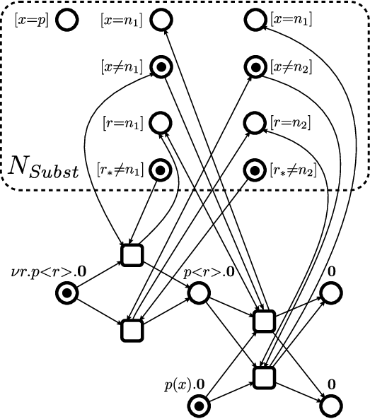
Fig. 4 shows the complete translation of the FCP $\nu r.\overline{p}\langle r\rangle.\mathbf{0}\mathop{|}p(x).\mathbf{0}$. The meanings of the places in $N_{\mathit{Subst}}$ are as in Fig. 3, and the places in the control flow are labelled by the corresponding subterms.

As the FCP has two bound names, $r$ and $x$, we take $\mathcal{N}=\{n_{1},n_{2}\}$. The initialisation of $r$ is represented by two transitions, corresponding to the values $n_{1}$ and $n_{2}$. The only possible communication in this example is between the prefixes $\overline{p}\langle r\rangle$ and $p(x)$. Note that the communication is over the public channel $p$, and the communicated values are from $\mathit{dom}(r)\cap\mathit{dom}(x)=\{n_{1},n_{2}\}\cap\{p,n_{1},n_{2}\}=\{n_{1},n_{2}\}$. Hence there are two transitions modelling this communication.

We augment the (NC) assumptions as follows: in a defining equation $K(\tilde{f}):=S$, $\mathit{fn}\left(S\right)=\tilde{f}$, i.e. public names are not allowed in $S$. This assumption can be enforced by passing the required public names as parameters.

To avoid case distinctions for the initial process, we assume there are artificial defining equations $K_{\mathit{Init},i}(\tilde{f}_{\mathit{Init},i}):=S_{\mathit{Init},i}$ with $\mathit{fn}\left(S_{\mathit{Init},i}\right)=\tilde{f}_{\mathit{Init},i}\subseteq\mathcal{F}$, that are called by a virtual initialisation step. Their purpose is to guarantee that the $S_{\mathit{Init},i}$ have the free names $\tilde{f}_{\mathit{Init},i}$. We then apply substitutions to assign the expected values to these parameters. This means we can write the given FCP as

where $\sigma_{i}:\tilde{f}_{\mathit{Init},i}\rightarrow\tilde{r}\cup\mathcal{P}$. We additionally assume that the $S_{\mathit{Init},i}$ are choices or calls and that the FCP does not contain the $\mathbf{0}$ process.

Moreover, if we have an input $x(y).S$ then we assume $y\in\mathit{fn}\left(S\right)$, which can be achieved by adding an artificial parameter to the call at the end of the process. Similarly, for a restriction $\nu r.S$ we assume $r\in\mathit{fn}\left(S\right)$. Restrictions not satisfying this requirement can be dropped due to structural congruence.

To represent a substitution like $\{a,b/x,y\}$, we decompose it into elementary substitutions $\{a/x\}\cup\{b/y\}$ of single names. The substitution net has corresponding places $[x{=}a]$ and $[y{=}b]$ for each elementary substitution that may occur in such a decomposition. Moreover, there is a second set of places, $[x{\neq}n]$ and $[r_{*}{\neq}n]$, keeping track of whether an input, a formal parameter, or a restriction is bound to $n\in\mathcal{N}$. These places complement the corresponding substitution places, in particular $[r_{*}{\neq}n]$ indicates that no restricted name is bound to $n$. (Since at most one restriction can be bound to $n$, this one complement place is sufficient.) $N_{\mathit{Subst}}$ has no transitions. We defer the explanation of its initial marking for the moment. Formally, $N_{\mathit{Subst}}\stackrel{{\scriptstyle\mbox{{\tiny\rm df}}}}{{=}}(P_{\mathit{Subst}}\cup P_{\mathit{Ref}},\emptyset,\emptyset,M_{0})$ with

Consider now a substitution $\sigma:(\mathcal{I}^{\prime}\cup\mathcal{F}^{\prime}\rightarrow\mathcal{P}\cup\tilde{r})\cup(\mathcal{R}^{\prime}\rightarrow\tilde{r})$ where $\mathcal{I}^{\prime}\subseteq\mathcal{I}$, $\mathcal{F}^{\prime}\subseteq\mathcal{F}$, $\mathcal{R}^{\prime}\subseteq\mathcal{R}$, and the second component $\mathcal{R}^{\prime}\rightarrow\tilde{r}$ is injective. A substitution marking $M$ of $N_{\mathit{Subst}}$ is said to correspond to $\sigma$ if the following hold:

1. (COR1): For all $x\in(\mathcal{I}\cup\mathcal{F}\cup\mathcal{R})\setminus\mathit{dom}(\sigma)$ and $a\in\mathcal{N}\cup\mathcal{P}$, $M([x{=}a])=0$.

2. (COR2): For all $x\in\mathit{dom}(\sigma)$ with $\sigma(x)\in\mathcal{P}$, $M([x{=}\sigma(x)])=1$.

3. (COR3): For all $x\in\mathit{dom}(\sigma)$ with $\sigma(x)\in\tilde{r}$, there is $n\in\mathcal{N}$ s.t. $M([x{=}n])=1$.

4. (COR4): The choice of $n$ preserves the equality of names as required by $\sigma$: for all $x,y\in\mathit{dom}(\sigma)$ with $\sigma(x),\sigma(y)\in\tilde{r}$, we have

   $$\sigma(x)=\sigma(y)\quad\text{iff}\quad\mbox{for all $n\in\mathcal{N}$,~}M([x{=}n])=M([y{=}n]).$$

Petri net $N(S_{\mathit{Init}})$ reflects the control flow of thread $S_{\mathit{Init}}$. To synchronise send and receive prefixes in different threads, we annotate its transitions with labels from

To capture the effect that reactions have on substitutions, transitions also carry a set of commands from

As $S_{\mathit{Init}}$ is a sequential process, transitions in $N(S_{\mathit{Init}})$ will always have a single input and a single output place. This allows us to understand $N(S_{\mathit{Init}})$ as a finite automaton, and hence define it implicitly via a new labelled transition system for $S_{\mathit{Init}}$. Recall that $\mathcal{S}$ is the set of sequential processes. We augment them by lists of names, $\mathcal{S}\times(\mathcal{I}\cup\mathcal{F}\cup\mathcal{R})^{*}$, carrying the names that have been forgotten and should be eventually unmapped in $N_{\mathit{Subst}}$. Among such augmented processes, we define the labelled transition relation

Each transition carries a label and a set of commands, and will yield a PN transition.

For restrictions $\nu r.S$, we allocate a fresh name. Since we can select any name that is not in use, such a transition exists for every $n\in\mathcal{N}$:

Fig. 5 depicts the transition, together with the implementation of mapping defined below.

Silent actions yield $\tau$-labelled transitions with empty sets of commands as expected:

where $\lambda^{\prime}=\mathit{fn}\left(\tau.S+\ldots\right)\setminus\mathit{fn}\left(S\right)$ contains the names that were free in the choice process but have been forgotten in $S$. With an ordering on $\mathcal{P}\cup\mathcal{N}$, we can understand this set as a sequence.

Communications are more subtle. Consider $\overline{x}\langle y\rangle.S+\ldots$ that sends $y$ on channel $x$. With appropriate tests, we find the names $a$ and $b$ to which $x$ and $y$ are mapped. These names then determine the transition label. So for all $a,b\in\mathcal{P}\cup\mathcal{N}$, we have

Sequence $\lambda^{\prime}$ again contains the names that have been forgotten during this step. A receive action in $x(y).S+\ldots$ is handled like a send, but introduces a new binding. For all $a,b\in\mathcal{P}\cup\mathcal{N}$, we have

References

- [1] R. Amadio and C. Meyssonnier. On decidability of the control reachability problem in the asynchronous -calculus. Nord. J. Comp., 9(1):70–101, 2002.
- [2] E. Best, R. Devillers, and M. Koutny. Petri Net Algebra. Monographs in Theoretical Computer Science. An EATCS Series. Springer, 2001.
- [3] N. Busi and R. Gorrieri. Distributed semantics for the -calculus based on Petri nets with inhibitor arcs. J. Log. Alg. Prog., 78(1):138––162, 2009.
- [4] M. Carbone and S. Maffeis. On the expressive power of polyadic synchronisation in pi-calculus. Nord. J. Comp., 10(2):70–98, 2003.
- [5] L. Cardelli and A. Gordon. Mobile ambients. In Proc. FOSSACS’98, volume 1378 of LNCS, pages 140–155. Springer, 1998.
- [6] M. Dam. Model checking mobile processes. Inf. Comp., 129(1):35–51, 1996.
- [7] R. Devillers, H. Klaudel, and M. Koutny. A compositional Petri net translation of general -calculus terms. For. Asp. Comp., 20(4–5):429–450, 2008.
- [8] C. Dufourd, A. Finkel, and Ph. Schnoebelen. Reset nets between decidability and undecidability. In Proc. of ICALP, volume 1443 of LNCS, pages 103–115. Springer, 1998.
- [9] J. Esparza. Decidability and complexity of Petri net problems—an introduction. In Lectures on Petri Nets I: Basic Models, volume 1491 of LNCS, pages 374–428. Springer, 1998.
- [10] G.-L. Ferrari, S. Gnesi, U. Montanari, and M. Pistore. A model-checking verification environment for mobile processes. ACM Trans. Softw. Eng. Methodol., 12(4):440–473, 2003.
- [11] R. Gorrieri and R. Meyer. On the relationship between pi-calculus and finite place/transition Petri nets. In Proc. of CONCUR, volume 5170 of LNCS, pages 463–480. Springer, 2009.
- [12] V. Khomenko, M. Koutny, and A. Niaouris. Applying Petri net unfoldings for verification of mobile systems. In Proc. of MOCA, Bericht FBI-HH-B-267/06, pages 161–178. University of Hamburg, 2006.
- [13] V. Khomenko and R. Meyer. Checking pi-calculus structural congruence is graph isomorphism complete. In S. Edwards, R. Lorenz, and W. Vogler, editors, Proc. ACSD’09, pages 70–79. IEEE Computing Society Press, 2009.
- [14] R. Meyer. On boundedness in depth in the -calculus. In Proc. of IFIP TCS, volume 273 of IFIP, pages 477–489. Springer, 2008.
- [15] R. Meyer. Structural Stationarity in the -calculus. PhD thesis, Department of Computing Science, University of Oldenburg, 2009.
- [16] R. Meyer. A theory of structural stationarity in the -calculus. Acta Inf., 46(2):87–137, 2009.
- [17] R. Meyer, V. Khomenko, and T. Strazny. A practical approach to verification of mobile systems using net unfoldings. Fundam. Inf., 94:439–471, 2009.
- [18] R. Milner. A Calculus of Communicating Systems. Springer, 1980.
- [19] R. Milner. Communicating and Mobile Systems: the -Calculus. CUP, 1999.
- [20] R. Milner, J. Parrow, and D. Walker. A calculus of mobile processes, part I. Inf. Comp., 100(1):1–40, 1992.
- [21] U. Montanari and M. Pistore. Checking bisimilarity for finitary -calculus. In Proc. of CONCUR, volume 962 of LNCS, pages 42–56. Springer, 1995.
- [22] F. Orava and J. Parrow. An algebraic verification of a mobile network. For. Asp. Comp., 4(6):497–543, 1992.
- [23] F. Peschanski, H. Klaudel, and R. Devillers. A Petri net interpretation of open reconfigurable systems. In Proc. of Petri nets’11, volume 6709, pages 208–227. Springer, 2011.
- [24] M. Pistore. History Dependent Automata. PhD thesis, Dipartimento di Informatica, Università di Pisa, 1999.
- [25] D. Sangiorgi and D. Walker. The -calculus: a Theory of Mobile Processes. CUP, 2001.
- [26] B. Victor and F. Moller. The mobility workbench: A tool for the -calculus. In Proc. of CAV, volume 818 of LNCS, pages 428–440. Springer, 1994.