跳到论文正文
W Papers独立论文阅读器 arXiv:1309.0624 论文正文 计算阅读时间 · 0%
引用这篇论文根据当前论文元数据生成,正式投稿前建议核对。


License: arXiv.org perpetual non-exclusive license
arXiv:1309.0624v2 [math.PR] 07 Oct 2013

Information Transmission under Random Emission Constraints

Francis Comets Note: comets@math.jussieu.fr; http://www.proba.jussieu.fr/$∼$comets    François Delarue Note: delarue@unice.fr; http://math.unice.fr/$∼$delarue    and René Schott(a) Laboratoire de Probabilités et Modèles Aléatoires,Université Paris Diderot-Paris 7, Case 7012, 75205 Paris Cedex 13, France.(b) Laboratoire J.-A. Dieudonné, Université de Nice Sophia-Antipolis,Parc Valrose, 06108 Nice Cedex 02, France.(c) IECL and LORIA, Université de Lorraine,54506 Vandoeuvre-lès-Nancy, France Note: schott@loria.fr; http://www.loria.fr/$∼$schott
Abstract

We model the transmission of a message on the complete graph with nn vertices and limited resources. The vertices of the graph represent servers that may broadcast the message at random. Each server has a random emission capital that decreases at each emission. Quantities of interest are the number of servers that receive the information before the capital of all the informed servers is exhausted and the exhaustion time. We establish limit theorems (law of large numbers, central limit theorem and large deviation principle), as n→∞n\to\infty, for the proportion of informed vertices before exhaustion and for the total duration. The analysis relies on a construction of the transmission procedure as a dynamical selection of successful nodes in a Galton-Watson tree with respect to the success epochs of the coupon collector problem.

Short Title: Information Transmission
Key words and phrases: Information transmission, epidemic model, complete graph, Galton-Watson tree, coupon collector problem, large deviations.
AMS subject classifications: Primary 90B30; secondary 05C81, 60F05, 60F10, 60J20, 92D30

1 Introduction

Transmission of information and dissemination of viruses in computer networks gave rise to many practical as well as theoretical investigations over the two last decades (see [4, 12, 19, 20, 23, 26]).

In this paper, we model the transmission of a message on the complete graph with nn vertices and limited ressources. Every vertex represents a server, which can be in one of three states: inactive (it did not receive the message yet), active (it has already received it, and is able to transmit it), exhausted (it has already received it, but cannot transmit it anymore because it has exhausted its own capital of emissions). Each server SiS_{i} has a random emission capital KiK_{i}. The message is initially received from outside by one server, which is then turned from the inactive state to the active one (if it has a positive emission capital) or exhausted (if its emission capital is 0), though the n−1n-1 other servers are inactive. At each integer time, one of the active servers (say SiS_{i}) casts the message, it looses one unit of its own emission capital KiK_{i}, and it selects the target at random among the nn servers. If the target is inactive, it discovers the information, it becomes itself active or exhausted according to its own emission capital. If not, this broadcast is unsuccessful and nothing else happens. When an active server exhausts its emission capital, it enters the exhausted state. The transmission ends at a finite time τn\tau_{n}, which is at most equal to 11 plus the sum of all initial capitals.

From a practical point, the graph may be thought as a wireless network, the vertices of which are battery powered sensors with a limited energy capacity. We refer the reader to [4, 12, 19, 20] for applications of graph theory to the performance evaluation of information transmission in wireless networks. We mention that the transmission process can be also interpreted as the busy period of a queue when the probability that a new customer enters the queue decays linearly as the number of past arrivals increases and finally vanishes after the nnth arrival.

Here we describe the asymptotic behavior of the proportion of informed vertices at the end of the process when nn tends to the infinity. The mathematical analysis relies on a twofold structure: a subtree of the Galton-Watson tree, which models the vertices reached by the emission procedure, and the success epochs of the coupon collector problem, which model the successful transmissions. Phrased in a probabilistic way, we propose a coupling of the transmission model as a marginal tree of the Galton-Watson tree, obtained by pruning some of the nodes according to the coupon collector problem. Such a coupling provides a direct interpretation of the scenarios when the network ceases broadcasting at the very beginning of the process: basically, these scenarios correspond to the extinction event in the Galton-Watson tree. On the survival event, we manage to specify the first-order behavior (in nn) of the exhaustion time τn\tau_{n} and of the proportion of informed nodes. Under suitable integrability conditions on the distribution of the capital of a given vertex, the fluctuations of both the exhaustion time and the proportion of informed nodes are also investigated: a central limit theorem is proved under a square-integrability condition and a somewhat involved large deviation principle is established under an exponential-integrability condition. In particular, when the distribution of the capital of a given vertex is of finite expectation, the probability that all the servers be reached before exhaustion (also referred to as the probability of full transmission) converges to 00 as nn tends to the infinity; as a consequence of the large deviation principle we prove here, it decays exponentially fast when the capital has a finite exponential moment. In some cases when the distribution of the capital has a heavy tail, we prove that the limit of the probability of full transmission is different from 00 and, in particular, may coincide with the entire probability of survival of the Galton-Watson tree. We refer to [5, 7, 13, 17, 21] and Chapter 8 of [31] for specific results concerning the coupon collector problem.

The papers [27] and [26] study closely related transmission models. Machado et al. [27] consider the case where Ki=2K_{i}=2 and prove partial transmission results. Obviously, our approach extends this result, as constant capitals are a particular case of random ones. A specific interest of random capitals consists in allowing KiK_{i} to be 00 with a non-trivial probability: as we shall see below, a quick stop of the transmission process then occurs with a positive probability, as the extinction event of the Galton-Watson tree. As in [27], Kurtz et al. [26] investigate the case where the KiK_{i}’s are constant, but possibly larger than 22, time running continuously. In their model, there is one particle at each vertex of the graph at time 0; one of them is active, the others are inactive. The active particle begins to move as a continuous-time, rate 1, random walk on the graph; as soon as any active particle visits an inactive one, the latter becomes active and starts an independent random walk. Each active particle dies at the instant it reaches a total of L jumps (consecutive or not) without activating any particle. Each active particle starts with L lives and looses one life unit whenever it jumps on a vertex which has already been visited by the process. For another similar model with simultaneous jumps in discrete time, the number of informed servers has fluctuations of order n3/4n^{3/4} [32].

We also emphasize that the dynamics of the present model is very similar, except for the asynchronisation, to the frog model on the complete graph with finite lifetimes: the earliest reference is [1], addressing the question of final coverage. In the frog model on ℤd{\mathbb{Z}}^{d}, there is a phase transition between almost-sure extinction and survival with positive probability according to the underlying death rate [2], and similarly for a time-continuous model [24]. Shape theorems are proved in [3], and also in [30] and [23] in continuous time. Fluctuations are Gaussian in one dimension [8, 9], but unknown when d≥2d\geq 2.

The paper is organized as follows. The basic model is presented in Section 2 together with the main results. In Section 3, we provide an alternative construction based on a pruning procedure of the Galton-Watson tree. Law of large numbers and related fluctuation limit theorems are investigated in Section 4, including the case of heavy tails. The large deviation principle is established in Section 5.

2 The model and main results

2.1 A Markovian definition of the dynamics

From a modeling point of view, we assume that the servers emit between consecutive integers. The global state of the whole system before and after emissions is thus described at integer times. At any time t∈ℕt\in{\mathbb{N}}, Nn​(t)N_{n}(t) denotes the number of servers which have already received the message and the so-called ‘total emission capital’ Sn​(t)S_{n}(t) the number of available attempts that can be used to deliver the message to a server which has not received it yet. At time 00, only one server detains the information. Its own capital, that is Sn​(0)S_{n}(0) with our notation, is a random variable, the distribution of which is denoted by μ\mu.

The dynamics of the pair process (Nn​(t),Sn​(t))t∈ℕ(N_{n}(t),S_{n}(t))_{t\in{\mathbb{N}}} are then assumed to be Markovian. Conditionally on the states up to time tt, the values of Nn​(t+1)N_{n}(t+1) and Sn​(t+1)S_{n}(t+1) are then given by:

Sn​(t+1)=Sn​(t)+{−1K⁡(t+1)−1​with​probability​{Nn​(t)/n1−Nn​(t)/n,S_{n}(t+1)=S_{n}(t)+\;\left\{\begin{array}[]{l}-1\\ K(t+1)-1\end{array}\right.\;{\rm with\ probability\ }\;\left\{\begin{array}[]{l}N_{n}(t)/n\\ 1-N_{n}(t)/n\end{array}\right., (1)

where K⁡(t+1)K(t+1) is a random variable, with μ\mu as distribution and independent of the past up until time tt; respectively, in the above cases,

Nn​(t+1)={Nn​(t)Nn​(t)+1​accordingly.N_{n}(t+1)=\;\left\{\begin{array}[]{l}N_{n}(t)\\ N_{n}(t)+1\end{array}\right.{\rm accordingly}. (2)

The Markov chain is absorbed at Sn=0S_{n}=0. From a practical point of view, the interpretation is the following. During the emission that occurs between times tt and t+1t+1, one server is chosen at random among the nn ones; it is referred to as the ‘target’. If the target is a server that has already received the information, then the number of informed servers remains the same and the total emission capital decreases by one. Such a scenario happens with the conditional probability Nn​(t)/nN_{n}(t)/n. If the target is a non-informed server, then the number of informed servers increases by one and the total emission capital increases by the own emission capital of the target which has just been activated. This happens with conditional probability 1−Nn​(t)/n1-N_{n}(t)/n and K⁡(t+1)K(t+1) then denotes the initial emission capital of the target activated between time tt and time t+1t+1. It is worth noting that the process (Nn​(t))t∈ℕ(N_{n}(t))_{t\in{\mathbb{N}}} is a Markov process itself, known as the ‘coupon collector process’ in the standard probability literature. It describes the collect, with replacement, of nn equally likely coupons.

With such a modeling, the variables K⁡(t),t∈ℕ,K(t),t\in{\mathbb{N}}, are i.i.d., with μ\mu as common distribution, K⁡(0)K(0) being equated with Sn​(0)S_{n}(0) and the sequences (K⁡(t))t∈ℕ(K(t))_{t\in{\mathbb{N}}} and (Nn​(t))t∈ℕ(N_{n}(t))_{t\in{\mathbb{N}}} being independent (we emphasize that, when the emission between tt and t+1t+1 is a failure, the variable K⁡(t+1)K(t+1) has no role in the description of the dynamics of the pair process (Nn​(t),Sn​(t))t∈ℕ(N_{n}(t),S_{n}(t))_{t\in{\mathbb{N}}}). By independence of the two sequences, the sum of all the capitals revealed up until time tt has the same law as R​(Nn​(t))R(N_{n}(t)) where

R⁡(t)=∑s=1tK⁡(s),t∈ℕ∖{0}.R(t)=\sum_{s=1}^{t}K(s),\quad t\in{\mathbb{N}}\setminus\{0\}. (3)

The transmission process lasts for a duration τn\tau_{n} which is the first time tt when the emission capital is equal to 0,

τn=min⁡{t∈ℕ:Sn​(t)=0}.\tau_{n}=\min\{t\in{\mathbb{N}}:S_{n}(t)=0\}. (4)

A natural question consists in determining whether the information will reach all servers, or a proportion of them only. We then define the event of full transmission,

𝚃𝚛𝚊𝚗𝚜n={Nn(τn)=n},{\tt Trans}_{n}=\{N_{n}(\tau_{n})=n\},

which occurs when all the servers finally receive the information. Then, three regimes of interest can be distinguished, according to

ℙ⁡(𝚃𝚛𝚊𝚗𝚜n)=0,or​ 1,or∈(0,1),{\mathbb{P}}({\tt Trans}_{n})=0,\;{\rm or}\;1,\;{\rm or}\;\in(0,1),

which naturally correspond to different tail behavior of KK. In all these cases, one is interested in the large-nn asymptotics of τn\tau_{n} and Nn​(τn)N_{n}(\tau_{n}).

Then, with the notation s∧t=min⁡{s,t}s\wedge t=\min\{s,t\}, the sequence (Sn​(t∧τn),Nn​(t∧τn))t∈ℕ(S_{n}(t\wedge\tau_{n}),N_{n}(t\wedge\tau_{n}))_{t\in{\mathbb{N}}} is a Markov chain on ℕ×{0,1,…,n}{\mathbb{N}}\times\{0,1,\ldots,n\} with a non-decreasing second component, and absorption on the vertical axis. The harmonic equations for absorption probabilities are rather intricate for a general KK, a natural route being to approximate the process by a differential equation. Here, our analysis will rely on a specific construction of the dynamics obtained by considering the Galton-Watson tree of reproduction law μ\mu.

2.2 Construction as a labeled Galton-Watson tree

In Section 3, we construct the information transmission process with a Galton-Watson tree with degree K∼μK\sim\mu and an independent coupon collector process with nn coupons. We only give a quick account here. For each nn, we prune the tree using the events of the nn-coupon collector. Given a realization of the Galton-Watson tree, we visit successively all the nodes starting from the root, we keep [resp., erase] the current node if a new coupon is obtained at that time [resp., if we do not collect a new coupon; then, the whole subtree below the current node is deleted]. This results into a subtree of the original one, with size Nn​(τn)≤nN_{n}(\tau_{n})\leq n.

Here is a precise statement. We denote by ZkGWZ_{k}^{\rm GW} the cardinality of the kk-th generation of the Galton-Watson tree and by 𝚂𝚞𝚛𝚟GW{\tt Surv}^{\rm GW} the survival event 𝚂𝚞𝚛𝚟GW={ZkGW≥1,∀k}{\tt Surv}^{\rm GW}=\{Z_{k}^{\rm GW}\geq 1,\forall k\}. It is well known that ℙ⁡(𝚂𝚞𝚛𝚟GW)>0{\mathbb{P}}({\tt Surv}^{\rm GW})>0 if and only if 𝔼​K>1{\mathbb{E}}K>1 or ℙ⁡(K=1)=1{\mathbb{P}}(K=1)=1.

Proposition 2.1

Let (Ω,𝒜,ℙ)(\Omega,{\mathcal{A}},{\mathbb{P}}) be a probability space where are defined: (i) a Galton-Watson tree with offspring distribution μ\mu, (ii) for each integer nn, a coupon collector process with nn coupons, independent of the tree.

Then, there exist sequences (Sn​(t),t∈ℕ)(S_{n}(t),t\in{\mathbb{N}}) and (Nn​(t),t∈ℕ)(N_{n}(t),t\in{\mathbb{N}}) defined on this probability space with Nn​(0)=1,Sn​(0)∼μN_{n}(0)=1,S_{n}(0)\sim\mu, and such that ((Nn​(t),Sn​(t)),t∈ℕ)((N_{n}(t),S_{n}(t)),t\in{\mathbb{N}}) is a Markov chain with transitions as in (1),(2).

Letting

ZtotGW=∑k≥0ZkGW,Z_{\rm tot}^{\rm GW}=\sum_{k\geq 0}Z_{k}^{\rm GW},

the full transmission event is ‘asymptotically included’ in the survival event in the sense that

𝚃𝚛𝚊𝚗𝚜n⊂{ZtotGW≥n}where{ZtotGW≥n}↘𝚂𝚞𝚛𝚟GWasn↗∞,{\tt Trans}_{n}\subset\left\{Z_{\rm tot}^{\rm GW}\geq n\right\}\quad{\rm where}\quad\left\{Z_{\rm tot}^{\rm GW}\geq n\right\}\searrow{\tt Surv}^{\rm GW}\;{\rm as}\;n\nearrow\infty,

and conversely, the event of termination at time o⁡(n)o(n) (o⁡(n)o(n) standing for the Landau notation) in the information process converges to extinction in the Galton-Watson process: denoting by Δ\Delta the symmetric difference,

limϵ→0+limn→∞ℙ({τn≥nϵ}Δ𝚂𝚞𝚛𝚟GW)=0.\lim_{\epsilon\to 0^{+}}\lim_{n\to\infty}{\mathbb{P}}\left(\{\tau_{n}\geq n\epsilon\}\Delta{\tt Surv}^{\rm GW}\right)=0. (5)

The construction is simple and natural, but it seems to be new and it turns out to be a powerful tool to analyze the information process. In all our results below, we consider this particular coupling of the information process with the Galton-Watson tree and the coupon collector.

2.3 Limit for the information coverage and duration

For 𝔼​K>1{\mathbb{E}}K>1, define θ∈(0,∞)\theta\in(0,\infty) as the unique root of the equation

1−e−θθ=1𝔼​K.\frac{1-e^{-\theta}}{\theta}=\frac{1}{{\mathbb{E}}K}. (6)

Extend this definition by setting θ=0​if​𝔼​K≤1,θ=∞​if​𝔼​K=∞.\theta=0{\rm\ if}\;{\mathbb{E}}K\leq 1,\theta=\infty{\rm\ if\ }{\mathbb{E}}K=\infty. The function 𝔼​K↦θ{\mathbb{E}}K\mapsto\theta is an increasing bijection from [0,∞][0,\infty] to [0,∞][0,\infty]. Let also

p=1−e−θ∈[0,1],p=1-e^{-\theta}\in[0,1], (7)

and note from (6), that when 𝔼​K∈(1,∞){\mathbb{E}}K\in(1,\infty), p=1−e−θ∈(0,1)p=1-e^{-\theta}\in(0,1) is the unique solution of

p​𝔼​K=−ln⁡(1−p),p\;{\mathbb{E}}K=-\ln(1-p), (8)

whereas p=1p=1 when θ=∞\theta=\infty. Let 𝟏A{\bf 1}_{A} denote the indicator function of the event AA.

Theorem 2.2

Let 𝔼​K∈(0,∞]{\mathbb{E}}K\in(0,\infty].

(i) As n→∞n\to\infty,

τn/n⟶θ​ 1𝚂𝚞𝚛𝚟GW\tau_{n}/n\longrightarrow\theta\;{\bf 1}_{{\tt Surv}^{\rm GW}}

in probability, with θ\theta defined by (6), though

Nn​(τn)/n⟶p​ 1𝚂𝚞𝚛𝚟GWN_{n}(\tau_{n})/n\longrightarrow p\;{\bf 1}_{{\tt Surv}^{\rm GW}}

in probability, with p=1−e−θp=1-e^{-\theta}.

(ii) If 𝔼​K≤1{\mathbb{E}}K\leq 1 (ℙ⁡(K=1)<1{\mathbb{P}}(K=1)<1 by assumption), then

limn→∞[τn+1]=limn→∞Nn​(τn)=ZtotGW\lim_{n\to\infty}\left[\tau_{n}+1\right]=\lim_{n\to\infty}N_{n}(\tau_{n})=Z_{\rm tot}^{\rm GW}

in probability.

As a straightforward consequence, we observe that ℙ⁡(𝚃𝚛𝚊𝚗𝚜n)→0{\mathbb{P}}({\tt Trans}_{n})\rightarrow 0 as n→∞n\rightarrow\infty whenever 𝔼​K{\mathbb{E}}K is finite, as pp is strictly less than 11 in this case. In Theorem 2.8 we shall prove that the rate of decay is exponential in the case when KK has a finite exponential moment.

2.4 Gaussian fluctuations in the case of a light tail

Theorem 2.3

Assume 𝔼​K>1{\mathbb{E}}K>1 and 𝔼​K2<∞{\mathbb{E}}K^{2}<\infty. Let σK2\sigma_{K}^{2} denote the variance of KK. As n→∞n\to\infty, conditionally on 𝚂𝚞𝚛𝚟GW{\tt Surv}^{\rm GW}, we have the convergence in law:

n−1/2(τn−nθ)⟶law𝒩(0,στ2),n^{-1/2}\big(\tau_{n}-n\theta\big)\stackrel{{\scriptstyle\rm law}}{{\longrightarrow}}{\mathcal{N}}(0,\sigma_{\tau}^{2}),

with στ2=[(1−p)​𝔼​K−1]−2​[p​σK2+(𝔼​K)2​σN​(θ)2]\sigma_{\tau}^{2}=[(1-p){\mathbb{E}}K-1]^{-2}[p\sigma_{K}^{2}+({\mathbb{E}}K)^{2}\sigma_{N}(\theta)^{2}] and σN​(s)2=e−s​(1−e−s)−s​e−2​s\sigma_{N}(s)^{2}=e^{-s}(1-e^{-s})-se^{-2s}. Similarly, conditionally on 𝚂𝚞𝚛𝚟GW{\tt Surv}^{\rm GW}, we have the convergence in law:

n−1/2(Nn(τn)−np)⟶law𝒩(0,σp2),n^{-1/2}\big(N_{n}(\tau_{n})-np\big)\stackrel{{\scriptstyle\rm law}}{{\longrightarrow}}{\mathcal{N}}(0,\sigma_{p}^{2}),

with σp2=[(1−p)​𝔼​K−1]−2​[p​σK2​e−2​θ+σN​(θ)2].\sigma_{p}^{2}=[(1-p){\mathbb{E}}K-1]^{-2}[p\sigma_{K}^{2}e^{-2\theta}+\sigma_{N}(\theta)^{2}].

Theorem 2.3 extends results in [26, 27]. We do not study the random fluctuations any further such as the corrections to the law of large numbers, but we prefer to explore the resulting regimes of full transmission. From Theorem 2.2, when 𝔼​K=∞{\mathbb{E}}K=\infty, Nn​(τn)/n→1N_{n}(\tau_{n})/n\to 1 in probability, conditionally on survival: This leaves open the asymptotics of the probability ℙ⁡(𝚃𝚛𝚊𝚗𝚜n){\mathbb{P}}({\tt Trans}_{n}). Some cases are investigated in the next subsection.

2.5 Probability of full transmission in the case of a heavy tail

When KK has a fat tail, fluctuations will serve the transmission process. The next result shows that the full transmission event converges to the survival event if the tail is very heavy.

Proposition 2.4

If there exist c>0c>0 and α∈(0,1)\alpha\in(0,1) such that lim infℓ→∞[ℓα​ℙ​(K≥ℓ)]≥c\liminf_{\ell\rightarrow\infty}[\ell^{\alpha}{\mathbb{P}}(K\geq\ell)]\geq c, then,

ℙ⁡(𝚃𝚛𝚊𝚗𝚜n)⟶ℙ⁡(𝚂𝚞𝚛𝚟GW)as​n→∞.{\mathbb{P}}({\tt Trans}_{n})\longrightarrow{\mathbb{P}}({\tt Surv}^{\rm GW})\quad{\rm as}\,n\rightarrow\infty.

Hence, fluctuations of sums of KK’s variables play a crucial role for the occurrence of full transmission. When μ\mu has a heavy tail, one of the servers activated during the transmission process has a large enough capital KK allowing it to contact all the other servers. We now turn to the critical case, when KK belongs to the domain of attraction of a stable law of index 1.

Theorem 2.5

Assume there exists c>0c>0 such that

ℙ⁡(K≥ℓ)∼cℓ,ℓ→∞.{\mathbb{P}}(K\geq\ell)\sim\frac{c}{\ell}\;,\qquad\ell\to\infty.

Then, as n→∞n\rightarrow\infty,

ℙ⁡(𝚃𝚛𝚊𝚗𝚜n)⟶ℙ⁡(𝚂𝚞𝚛𝚟GW)×{𝔼⁡(exp⁡(−e−𝒮)),c=1,1,c>1,0,c<1,{\mathbb{P}}({\tt Trans}_{n})\longrightarrow{\mathbb{P}}({\tt Surv}^{\rm GW})\times\left\{\begin{array}[]{ll}{\mathbb{E}}(\exp(-e^{-{\mathcal{S}}}))\;,&c=1,\\ 1\;,&c>1,\\ 0\;,&c<1,\end{array}\right.

where, in the case c=1c=1, 𝒮=limn→∞n−1​(R⁡(n)−n​ln⁡n){\mathcal{S}}=\lim_{n\to\infty}n^{-1}(R(n)-n\ln n) is a totally asymmetric Cauchy variable, the centering parameter of which depends on the distribution of KK (see (3) for the definition of RR).

The particular form of the limit relates to the celebrated result of Erdös and Rényi [16] for the coupon collector, that is the time to collect all coupons has a Gumbel limit law.

2.6 Large deviations

Following Chapter 1 in [11], we recall that a random sequence (Zn,n≥1)(Z_{n},n\geq 1), with values in some Polish space 𝒵\mathcal{Z}, obeys a large deviation principle (LDP) with rate function ℐ\mathcal{I} and speed nn if
  ∙\bullet ℐ:𝒵→[0,∞]{\mathcal{I}}:{\mathcal{Z}}\to[0,\infty] is lower semi-continuous;
  ∙\bullet for all closed subset F⊂𝒵F\subset{\mathcal{Z}}, lim supn→∞n−1lnℙ(Zn∈F)≤−inf{ℐ(z);z∈F}\limsup_{n\to\infty}n^{-1}\ln{\mathbb{P}}(Z_{n}\in F)\leq-\inf\{{\mathcal{I}}(z);z\in F\};
  ∙\bullet for all open subset O⊂𝒵O\subset{\mathcal{Z}}, lim infn→∞n−1lnℙ(Zn∈O)≥−inf{ℐ(z);z∈O}\liminf_{n\to\infty}n^{-1}\ln{\mathbb{P}}(Z_{n}\in O)\geq-\inf\{{\mathcal{I}}(z);z\in O\}.

Assume all through this section that KK has exponentially small tails: 𝔼​exp⁡(a0​K)<∞{\mathbb{E}}\exp(a_{0}K)<\infty for some a0>0.a_{0}>0. Then, by Cramer’s theorem (e.g., Subsection 2.2.1 in [11]), R⁡(n)/nR(n)/n obeys a LDP with rate II,

I⁡(u)=sup{a​u−ln⁡𝔼​exp⁡(a​K);a∈ℝ},u∈[0,∞),I(u)=\sup\{au-\ln{\mathbb{E}}\exp(aK);a\in{\mathbb{R}}\},\qquad u\in[0,\infty), (9)

and I⁡(u)=∞I(u)=\infty for u<0u<0. The function II is convex, lower semicontinuous and has compact level sets {u∈ℝ:I⁡(u)≤c}\{u\in{\mathbb{R}}:I(u)\leq c\}, for c∈[0,∞)c\in[0,\infty). The domain of the rate function II is defined as the set Dom​(I)\textrm{Dom}(I) of reals uu with finite I⁡(u)I(u). Here, we have Dom​(I)=[k∗,k∗]​⋂ℝ\textrm{Dom}(I)=[k_{*},k^{*}]\bigcap{\mathbb{R}}, with

k∗=min⁡{k:ℙ⁡(K=k)>0},k∗=sup{k:ℙ⁡(K=k)>0}.k_{*}=\min\{k:{\mathbb{P}}(K=k)>0\},\qquad k^{*}=\sup\{k:{\mathbb{P}}(K=k)>0\}.

We also recall the large deviations principle for the coupon collector process with nn coupons from Boucheron et al. [7], Dupuis et al. [13]: for all t>0t>0, we have:

Nn​(n​t)/nobeys​a​LDP​with​speed​n​and​rate​function​Jt.N_{n}(nt)/n\quad{\rm obeys\ a\ LDP\ with\ speed\ }n{\rm\ and\ rate\ function\ }J_{t}. (10)

From (2.7) and Section 4.1 in [13], the rate function JtJ_{t} is convex, it is finite if and only if r∈(0,t∧1]r\in(0,t\wedge 1], with limr↘0Jt​(r)=∞\lim_{r\searrow 0}J_{t}(r)=\infty, and it has a finite limit as r→t∧1r\to t\wedge 1. For r∈(0,t∧1)r\in(0,t\wedge 1), it is given by

Jt​(r)=(1−r)​ln⁡(1−r)+(t−r)​ln⁡ρ⁡(r,t)+t​e−t​ρ​(r,t),J_{t}(r)=(1-r)\ln(1-r)+(t-r)\ln\rho(r,t)+te^{-t\rho(r,t)}, (11)

where ρ⁡(r,t)\rho(r,t) denotes the unique solution in (0,∞)(0,\infty) of

1−e−t​ρρ=r.\frac{1-e^{-t\rho}}{\rho}=r. (12)

With these ingredients we define the function ℱ:ℝ+2→[0,∞]{\mathcal{F}}:{\mathbb{R}}_{+}^{2}\to[0,\infty] by

ℱ⁡(r,t)={r​I​(t/r)+Jt​(r)ifr>0,∞ifr=0,t>0,0ifr=t=0.{\mathcal{F}}(r,t)=\left\{\begin{array}[]{lll}rI(t/r)+J_{t}(r)&{\rm if}&r>0,\\ \infty&{\rm if}&r=0,\ t>0,\\ 0&{\rm if}&r=t=0.\end{array}\right. (13)
Lemma 2.6

(i) The function ℱ{\mathcal{F}}, is lower semi-continuous on ℝ+2{\mathbb{R}}_{+}^{2} with compact level sets {(r,t):ℱ⁡(r,t)≤c}\{(r,t):{\mathcal{F}}(r,t)\leq c\} for nonnegative cc. Its domain is equal to

Dom(ℱ)={(r,t)∈ℝ+2:0<r≤t∧1,(k∗∨1)r≤t≤k∗r}∪{(0,0)}.{\rm Dom}({\mathcal{F}})=\Big\{(r,t)\in{\mathbb{R}}_{+}^{2}:0<r\leq t\wedge 1,(k_{*}\vee 1)r\leq t\leq k^{*}r\Big\}\cup\Big\{(0,0)\Big\}.

It is continuous on Dom⁡(ℱ)∖{(0,0)}{\rm Dom}({\mathcal{F}})\setminus\{(0,0)\}. It is continuous at the origin if and only if KK is bounded.

(ii) Moreover,

ℱ⁡(1−e−t,t)=(1−e−t)​I​(t1−e−t),{\mathcal{F}}\bigl(1-e^{-t},t\bigr)=(1-e^{-t})I\biggl(\frac{t}{1-e^{-t}}\biggr),

and when k∗≤1<k∗k_{*}\leq 1<k^{*}, we have ℱ⁡(1−e−t,t)∼t​I​(1){\mathcal{F}}(1-e^{-t},t)\sim tI(1) as t→0t\rightarrow 0.

(iii) When 𝔼​K>1{\mathbb{E}}K>1, the function ℱ{\mathcal{F}} is not convex, as it takes the value 0 at points (p,θ)(p,\theta) and (0,0)(0,0), and is positive elsewhere. When 𝔼​K≤1{\mathbb{E}}K\leq 1, ℱ{\mathcal{F}} is positive everywhere except at 0.

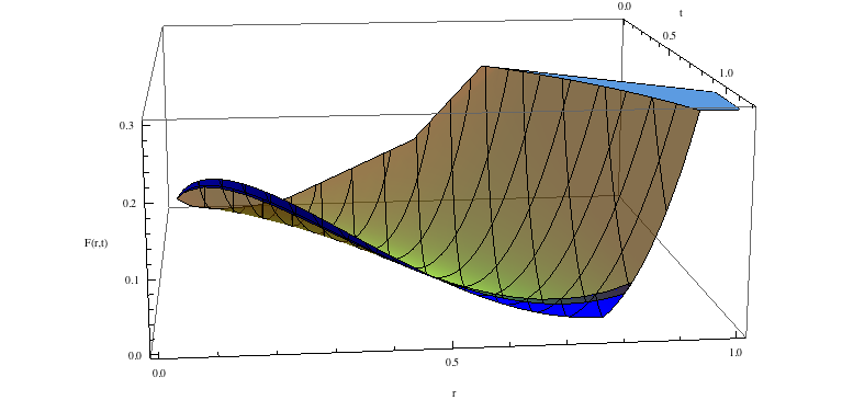
The domain of ℱ{\mathcal{F}} might be rather degenerated. For example, in the Bernoulli case K∈{0,1}K\in\{0,1\}, it reduces to the segment {(r,r),0≤r≤1}\{(r,r),0\leq r\leq 1\}. This function is an intricate combination of the rate functions of the coupon collector process and of the Galton-Watson process. This makes it an interesting rate function in its own. The shape of the graph of ℱ{\mathcal{F}} is shown in Figure 1 in the case 𝔼​K>1{\mathbb{E}}K>1.

Theorem 2.7

The sequence (n−1​(Nn​(τn),τn),n≥1)\big(n^{-1}(N_{n}(\tau_{n}),\tau_{n});{n\geq 1}\big) obeys a LDP with rate function ℱ{\mathcal{F}} and speed nn.

As a corollary, we obtain a variational formula for the probability of full transmission.

Theorem 2.8

The decay of the probability for all servers to be reached before exhaustion is exponential and given by:

limn→+∞n−1lnℙ(𝚃𝚛𝚊𝚗𝚜n)=−infs≥0{I(λ(s))+(λ(s)−1)ln(−e−s)+λ(s)e−s},\lim_{n\rightarrow+\infty}n^{-1}\ln{\mathbb{P}}({\tt Trans}_{n})=-\inf_{s\geq 0}\Bigl\{I\bigl(\lambda(s)\bigr)+(\lambda(s)\!-\!1)\ln\bigl(1\!-\!e^{-s}\bigr)+\lambda(s)e^{-s}\Bigr\},

with λ⁡(s)=s/(−e−s)\lambda(s)=s/(1\!-\!e^{-s}) for s>0,s>0, and λ⁡(0)=1\lambda(0)=1. The above right-hand side is negative.
Refer to caption
Figure 1: Rate function ℱ{\mathcal{F}} for KK Poisson distributed with mean 1.4998. It vanishes at the origin and at (p,θ)=(.5827,.8740)(p,\theta)=(.5827,.8740), it is unbounded in neighborhoods of (0,0)(0,0) in its domain. For convenience, large values of ℱ{\mathcal{F}} are truncated, and the graph over the domain r≤.65​tr\leq.65t is not shown. The dark blue strip corresponds to .65​t≤r≤.67​t.65t\leq r\leq.67t, and the yellow part of the graph to r≥.67​tr\geq.67t.

3 Construction from a labeled Galton-Watson tree

Let 𝒲=∪k≥0(ℕ∗)k{\mathcal{W}}=\cup_{k\geq 0}({\mathbb{N}}^{*})^{k} be the set of all finite words on the alphabet {1,2,…}\{1,2,\ldots\}. Its elements are of the form w1​w2​…​wk,wi∈ℕ∗w_{1}w_{2}\ldots w_{k},w_{i}\in{\mathbb{N}}^{*} when k≥1k\geq 1, and, for k=0k=0, (ℕ∗)k({\mathbb{N}}^{*})^{k} reduces to the empty word ∅{\varnothing}, that we call the root. We then denote by |w|=k|w|=k the length of w=w1​w2​…​wk∈𝒲w=w_{1}w_{2}\dots w_{k}\in{\mathcal{W}} (with |∅|=0|{\varnothing}|=0.) For w,w′∈𝒲w,w^{\prime}\in{\mathcal{W}}, we write w<w′w<w^{\prime} if: |w|<|w′||w|<|w^{\prime}|, or |w|=|w′||w|=|w^{\prime}| and w≤lexw′w{\leq}_{\rm lex}w^{\prime} in the lexicographic order. We denote by ≼\preccurlyeq the usual predecessor relation in 𝒲{\mathcal{W}}, that is w≼w′w\preccurlyeq w^{\prime} if ww is a prefix of w′w^{\prime}.

Let (K⁡(w),w∈𝒲)(K(w),w\in{\mathcal{W}}) be a family of i.i.d. random variables on ℕ={0,1,2,…}{\mathbb{N}}=\{0,1,2,\ldots\} with common law μ\mu (pay attention that the notation K⁡(t),t∈ℕK(t),t\in{\mathbb{N}}, is also used in Subsection 2.1; we here use the same letter KK, but a different index, no confusion being possible in the sequel). Assume μ⁡(0)<1\mu(0)<1 and μ⁡(1)<1\mu(1)<1 for a nontrivial setup. The associated Galton-Watson tree 𝒯GW{\mathcal{T}^{\rm GW}} is the set of w∈𝒲w\in{\mathcal{W}} such that w=∅w={\varnothing} or, for all i=1,…,|w|,wi≤K⁡(v)i=1,\ldots,|w|,w_{i}\leq K(v) with vv the predecessor of ww of length i−1i-1 (in other words, given a parent w′w^{\prime} at the (i−1)(i-1)th generation, that is w′w^{\prime} is a word of length i−1i-1, the children of w′w^{\prime} are the words w′​1w^{\prime}1, …\dots, w′​K​(w′)w^{\prime}K(w^{\prime}), of length ii, obtained by concatenation). Denote by ZkGWZ^{\rm GW}_{k} the size of the kkth generation of this tree, ZkGW=𝚌𝚊𝚛𝚍⁡{w∈𝒯GW:|w|=k}Z^{\rm GW}_{k}={\tt card}\;\{w\in{\mathcal{T}^{\rm GW}}:|w|=k\}, which is given by

Zk+1GW=∑v∈𝒯GW,|v|=kK⁡(v),Z0GW=1.Z^{\rm GW}_{k+1}=\sum_{v\in{\mathcal{T}^{\rm GW}},|v|=k}K(v),\quad Z^{\rm GW}_{0}=1.

Recalling that μ⁡(1)<1\mu(1)<1, it is well known that the survival event 𝚂𝚞𝚛𝚟GW=⋂k{ZkGW≥1}={𝚌𝚊𝚛𝚍𝒯GW=∞}{\tt Surv}^{\rm GW}=\bigcap_{k}\{Z^{\rm GW}_{k}\geq 1\}=\{{\tt card}\;{\mathcal{T}^{\rm GW}}=\infty\} has complement probability

σGW=1−ℙ⁡(𝚂𝚞𝚛𝚟GW)={=1if​𝔼​K≤1,<1if​𝔼​K>1.\sigma^{\rm GW}=1-{\mathbb{P}}({\tt Surv}^{\rm GW})=\left\{\begin{array}[]{ll}=1&{\rm if}\;{\mathbb{E}}K\leq 1,\\ <1&{\rm if}\;{\mathbb{E}}K>1.\end{array}\right.

On the same probability space, we consider an independent coupon collector process with nn images (n≥1n\geq 1): Let Δi,n\Delta_{i,n}, i=1,…​n−1i=1,\ldots n-1, be independent, geometrically distributed r.v.’s on ℕ∗{\mathbb{N}}^{*} with parameter 1−i/n1-i/n (success probability) respectively. The success epochs are

T1,n=0,Ti,n=∑j=1i−1Δj,n,i=2,…n,T_{1,n}=0,\qquad T_{i,n}=\sum_{j=1}^{i-1}\Delta_{j,n},\qquad i=2,\ldots n,

and the counting function is

Nn(t)=∑i=1n𝟏{Ti,n≤t},t=0,1,…N_{n}(t)=\sum_{i=1}^{n}{\bf 1}_{\{T_{i,n}\leq t\}},\qquad t=0,1,\ldots

In fact, Nn​(t)N_{n}(t) represents the number of servers having received the information by time tt (note that 1≤Nn​(t)≤(t+1)∧n1\leq N_{n}(t)\leq(t+1)\wedge n).

For any fixed integer nn, with these two ingredients, we can define the transmission process together with the transmission time length τn\tau_{n}. Let us start with an informal description. We browse a part of the Galton-Watson tree following the order <<, and we paint the nodes in ∘\circ or in △{\triangle} according to the coupon collector process (success or failure); we only browse nodes which are in stand-by; as soon as a node is painted in ∘\circ, its number of children nodes in 𝒯GW{\mathcal{T}^{\rm GW}} is revealed, and these children are put in stand-by. We then move to the next node in stand-by (next for <<). The procedure runs until there are no nodes in stand-by anymore.

Here is a precise definition. Recursively for t=0,1,…t=0,1,\ldots, we construct X⁡(t)∈𝒯GWX(t)\in{\mathcal{T}^{\rm GW}}, and disjoint 𝒯∘​(t),𝒯⊠​(t),𝒯△​(t)⊂𝒯GW{\mathcal{T}^{\circ}}(t),{\mathcal{T}^{\boxtimes}}(t),{\mathcal{T}^{\vartriangle}}(t)\subset{\mathcal{T}^{\rm GW}} as follows (X⁡(t)X(t) encodes the vertex where the ttth tentative emission takes place, 𝒯∘​(t){\mathcal{T}^{\circ}}(t) denotes the set of servers already informed by time tt, 𝒯⊠​(t){\mathcal{T}^{\boxtimes}}(t) is the set of tentative emissions scheduled but not yet performed at time tt, 𝒯△​(t){\mathcal{T}^{\vartriangle}}(t) is set of failed emissions, i.e. those performed before time tt for which the target was already informed). Start with

X(0)=∅,𝒯∘(0)={∅},𝒯⊠(0)={w∈𝒯GW:|w|=1,1≤w1≤K(∅)},𝒯△(0)=∅.X(0)={\varnothing},\quad{\mathcal{T}^{\circ}}(0)=\{{\varnothing}\},\quad{\mathcal{T}^{\boxtimes}}(0)=\{w\in{\mathcal{T}^{\rm GW}}:|w|=1,1\leq w_{1}\leq K({\varnothing})\},\quad{\mathcal{T}^{\vartriangle}}(0)=\emptyset.

Here, and below, ∅\emptyset denotes the empty set and will not be confused with the root ∅{\varnothing} of the tree. With the process (X⁡(t),𝒯∘​(t),𝒯⊠​(t),𝒯△​(t))(X(t),{\mathcal{T}^{\circ}}(t),{\mathcal{T}^{\boxtimes}}(t),{\mathcal{T}^{\vartriangle}}(t)) at time tt, its value at the next step t+1t+1 is defined by:

  • •

    If 𝒯⊠​(t){\mathcal{T}^{\boxtimes}}(t) is nonempty, we let X⁡(t+1)X(t+1) be its first element,

    X(t+1)=inf{w∈𝒯⊠(t)},denotedbyvX(t+1)=\inf\{w\in{\mathcal{T}^{\boxtimes}}(t)\},\;{\rm denoted\ by}\;v

    to ease the notations, and we perform a test:

    • –

      If Nn​(t+1)=Nn​(t)+1N_{n}(t+1)=N_{n}(t)+1, we define

      𝒯∘​(t+1)=𝒯∘​(t)∪{v},𝒯⊠​(t+1)=(𝒯⊠​(t)∖{v})∪{v​1,v​2,…,v​K​(v)},𝒯△​(t+1)=𝒯△​(t),\begin{array}[]{l}{\mathcal{T}^{\circ}}(t+1)={\mathcal{T}^{\circ}}(t)\cup\{v\},\\ {\mathcal{T}^{\boxtimes}}(t+1)=\big({\mathcal{T}^{\boxtimes}}(t)\setminus\{v\}\big)\cup\big\{v1,v2,\ldots,vK(v)\big\},\\ {\mathcal{T}^{\vartriangle}}(t+1)={\mathcal{T}^{\vartriangle}}(t),\end{array} (14)

      the notation v​kvk denoting the word of length |v|+1|v|+1 obtained by concatenation.

    • –

      If Nn​(t+1)=Nn​(t)N_{n}(t+1)=N_{n}(t), we define

      𝒯∘​(t+1)=𝒯∘​(t),𝒯⊠​(t+1)=𝒯⊠​(t)∖{v},𝒯△​(t+1)=𝒯△​(t)∪{v}.\begin{array}[]{l}{\mathcal{T}^{\circ}}(t+1)={\mathcal{T}^{\circ}}(t),\\ {\mathcal{T}^{\boxtimes}}(t+1)={\mathcal{T}^{\boxtimes}}(t)\setminus\{v\},\\ {\mathcal{T}^{\vartriangle}}(t+1)={\mathcal{T}^{\vartriangle}}(t)\cup\{v\}.\end{array} (15)
  • •

    If 𝒯⊠​(t){\mathcal{T}^{\boxtimes}}(t) is empty, we set τn=t\tau_{n}=t, and the construction is stopped (as well as the transmission). The set 𝒯∘​(t)=𝒯∘​(τn)=𝒯∘​(∞){\mathcal{T}^{\circ}}(t)={\mathcal{T}^{\circ}}(\tau_{n})={\mathcal{T}^{\circ}}(\infty) is the set of servers finally informed. Note that τn≤Tn,n\tau_{n}\leq T_{n,n} is a.s. finite.

We observe that for all tt, 𝒯∘​(t){\mathcal{T}^{\circ}}(t) is a tree, as well as 𝒯∘​(t)∪𝒯⊠​(t){\mathcal{T}^{\circ}}(t)\cup{\mathcal{T}^{\boxtimes}}(t). Moreover, 𝒯⊠​(t)∪𝒯△​(t){\mathcal{T}^{\boxtimes}}(t)\cup{\mathcal{T}^{\vartriangle}}(t) is a cutset of 𝒯GW{\mathcal{T}^{\rm GW}} for its own graph structure.

∅ X ( + t 1 ) Figure 2. The Galton-Watson tree is represented up to the 4th generation., and and are represented at time . ⁢ T ∘ ( t ) ⁢ T ⊠ ( t ) ⁢ T △ ( t ) X ( + t 1 ) = t 10

Figure 2 provides an example of construction of the sets 𝒯∘​(t){\mathcal{T}^{\circ}}(t), 𝒯⊠​(t){\mathcal{T}^{\boxtimes}}(t) and 𝒯△​(t){\mathcal{T}^{\vartriangle}}(t), t∈{0,1,…,10}t\in\{0,1,\dots,10\}, according to the rules prescribed in (14) and (15). At time 00, the capital of the initial server is K⁡(∅)=4K({\varnothing})=4, so that the root of the tree has four children. Between times 00 and 11, the first emission is a success as the server which is revealed in the tree is painted in ∘\circ. This server reads as the first child (starting from the left) at the first generation of the tree; it has two children, that is K⁡(‘1’)=2K(\textrm{`1'})=2, where ‘1’ is here understood as a one-letter word. At time 11, the total emission capital is thus S⁡(1)=4+2−1=5S(1)=4+2-1=5, and 𝒯⊠​(2){\mathcal{T}^{\boxtimes}}(2) contains the three last children at the first generation and the two first children at the second generation. Since the second child at the first generation is painted in △\triangle, the emission between times 11 and 22 fails, which means that the children of this node are not considered for the sequel of the construction. At time 22, S⁡(2)=4+2−2=4S(2)=4+2-2=4. Then, the emission between times 22 and 33 is a success but the server which is informed has no children (third child in the first generation) and the emission between times 33 and 44 is a success as well, with K⁡(‘4’)=3K(\textrm{`4'})=3. At time 44, 𝒯⊠​(4){\mathcal{T}^{\boxtimes}}(4) contains 5 nodes, all of them at the second generation of the tree. The node X⁡(5)X(5) is then the first child at the second generation: as it is painted in △\triangle, the emission between times 44 and 55 fails. And so on up until time 1010. Then, 𝒯⊠​(10){\mathcal{T}^{\boxtimes}}(10) contains 5 nodes: two of them at the fourth generation and three of them at the third generation. With the lexicographic order, X⁡(11)=‘411’X(11)=\textrm{`411'}.

We now relate the above construction to the dynamical model for transmission. Let 𝚌𝚊𝚛𝚍​A{\tt card}\;A denote the cardinality of a set AA. Consider a new, independent, i.i.d. sequence (K¯i)i≥1(\bar{K}_{i})_{i\geq 1} with law μ\mu, and define, for i=1,…​ni=1,\ldots n,

Ki={K⁡(X⁡(Ti,n))if​i≤𝚌𝚊𝚛𝚍​𝒯∘​(∞),K¯iif​i>𝚌𝚊𝚛𝚍​𝒯∘​(∞),K_{i}=\left\{\begin{array}[]{ll}K(X(T_{i,n}))&{\rm if}\;i\leq{\tt card}\;{\mathcal{T}^{\circ}}(\infty),\\ \bar{K}_{i}&{\rm if}\;i>{\tt card}\;{\mathcal{T}^{\circ}}(\infty),\end{array}\right. (16)

and also

Sn​(t):=∑i=1Nn​(t)Ki−t,t∈ℕ∖{0}.S_{n}(t):=\sum_{i=1}^{N_{n}(t)}K_{i}-t,\quad t\in{\mathbb{N}}\setminus\{0\}. (17)

Below, we also write

Sn(t)=R(Nn(t))−t,t∈ℕ,withR(m):=∑i=1mKi,m∈ℕ∖{0}.S_{n}(t)=R\left(N_{n}(t)\right)-t,\quad t\in{\mathbb{N}},\quad\textrm{with}\quad R(m):=\sum_{i=1}^{m}K_{i},\quad m\in{\mathbb{N}}\setminus\{0\}. (18)

Pay attention that the letter RR is also used in (3), but as proved right below the two RR’s have the same distribution. In the sequel, we will always refer to (18) for the precise definition of RR.

By construction, we have

Nn​(t)=𝚌𝚊𝚛𝚍​𝒯∘​(t),Sn​(t)=𝚌𝚊𝚛𝚍​𝒯⊠​(t).N_{n}(t)={\tt card}\;{\mathcal{T}^{\circ}}(t),\quad S_{n}(t)={\tt card}\;{\mathcal{T}^{\boxtimes}}(t). (19)
Proposition 3.1

The variables (Ki)1≤i≤n(K_{i})_{1\leq i\leq n} are independent, identically distributed with law μ\mu, and (Ki)1≤i≤n(K_{i})_{1\leq i\leq n} is independent of (Ti,n)1≤i≤n(T_{i,n})_{1\leq i\leq n}. Moreover,

τn=min⁡{t∈ℕ:Sn​(t)=0}.\tau_{n}=\min\{t\in{\mathbb{N}}:S_{n}(t)=0\}. (20)

Proof: The formula for τn\tau_{n} directly follows from (19), and the fact that τn\tau_{n} is finite. We now investigate the distribution of the sequence (Ki,i≤n)(K_{i},i\leq n). Below, we denote by ℱw=σ⁡(K⁡(w′),w′≤w){\mathcal{F}}_{w}=\sigma(K(w^{\prime}),w^{\prime}\leq w) for w∈𝒲w\in{\mathcal{W}}. On the event A={(T1,n,…,Ti,n)=(k1,…,ki),X⁡(ki−1)=w,τn≥ki}A=\{(T_{1,n},\dots,T_{i,n})=(k_{1},\dots,k_{i}),X(k_{i}-1)=w,\tau_{n}\geq k_{i}\}, 0=k1<⋯<ki0=k_{1}<\dots<k_{i} and w∈𝒲w\in{\mathcal{W}}, |w|≤ki−1|w|\leq k_{i}-1, X⁡(Ti,n)X(T_{i,n}) coincides with an ℱw{\mathcal{F}}_{w}-measurable r.v., denoted by χ\chi, which satisfies w<χw<\chi almost-surely (this follows from the monotonicity of the browsing procedure). Similarly, all the variables K⁡(X⁡(Tj,n))K(X(T_{j,n})), 1≤j≤i−11\leq j\leq i-1 coincide with ℱw{\mathcal{F}}_{w}-measurable r.v.’s on AA. Clearly, K⁡(χ)K(\chi) is independent of ℱw∨σ⁡(T1,n,…,Tn,n){\mathcal{F}}_{w}\vee\sigma(T_{1,n},\dots,T_{n,n}) and has μ\mu as distribution, since the r.v.’s (K⁡(w′),w′∈𝒲)(K(w^{\prime}),w^{\prime}\in{\mathcal{W}}) are i.i.d and are independent of the success epochs (T1,n,…,Tn,n)(T_{1,n},\dots,T_{n,n}). Obviously, the event AA belongs to ℱw∨σ⁡(T1,n,…,Tn,n){\mathcal{F}}_{w}\vee\sigma(T_{1,n},\dots,T_{n,n}). This proves that, for any bounded and measurable Borel function ϕ\phi,

𝔼[ϕ(Ki)𝟏{Ti,n≤τn}|(Tj,n,1≤j≤n),(Kj,1≤j≤i−1)]=𝟏{Ti,n≤τn}∫ℕϕdμ.{\mathbb{E}}\bigl[\phi(K_{i}){\mathbf{1}}_{\{T_{i,n}\leq\tau_{n}\}}|(T_{j,n},1\leq j\leq n),(K_{j},1\leq j\leq i-1)\bigr]={\mathbf{1}}_{\{T_{i,n}\leq\tau_{n}\}}\int_{\mathbb{N}}\phi d\mu.

On the event {(T1,n,…,Ti,n)=(k1,…,ki),τn<ki}\{(T_{1,n},\dots,T_{i,n})=(k_{1},\dots,k_{i}),\tau_{n}<k_{i}\}, KiK_{i} coincides with K¯i\bar{K}_{i}, which is obviously independent of σ((Tj,n,1≤j≤n),(Kj,1≤j≤i−1))\sigma((T_{j,n},1\leq j\leq n),(K_{j},1\leq j\leq i-1)), so that the above equality also holds with Ti,n≤τnT_{i,n}\leq\tau_{n} replaced by Ti,n>τnT_{i,n}>\tau_{n}. □\Box

Then the process we have constructed here corresponds to the description of the information transmission process given in Subsection 2.1.

Proof of Proposition 2.1: (5) follows from Lemma 4.2 below and {τn≥nϵ}⊂{ZtotGW≥nϵ}\{\tau_{n}\geq n\epsilon\}\subset\{Z_{\rm tot}^{\rm GW}\geq n\epsilon\}. The other claims directly follow from the construction and Proposition 3.1. □\Box

4 Proofs of law of large numbers and fluctuations

In all the proofs, we use the following convention: for any discrete process (Vt,t∈ℕ)(V_{t},t\in{\mathbb{N}}), (Vt,t≥0)(V_{t},t\geq 0) stands for (V⌊t⌋,t≥0)(V_{\lfloor t\rfloor},t\geq 0), where ⌊⋅⌋\lfloor\cdot\rfloor is the floor function. We will also use the ceiling function, denoted by ⌈⋅⌉\lceil\cdot\rceil. For an interval II in ℝ{\mathbb{R}}, define the Skorokhod space D⁡(I)D(I) as the space of càdlàg (right continuous left limited) functions from II to ℝ{\mathbb{R}}.

4.1 Proofs of the law of large numbers

Lemma 4.1

We have the following convergence in law of sequences of processes on the Skorohod space (endowed with the standard J1 topology, keeping in mind that convergence for the J1 topology implies uniform convergence on compacts when the limit function is continuous):

(i) On D⁡([0,1))D([0,1)),

n−1/2(T⌊n​q⌋,n−nln11−q)0≤q<1⟶law[B(σT(q)2)]0≤q<1asn→∞,n^{-1/2}\big(T_{\lfloor nq\rfloor,n}-n\ln\frac{1}{1-q}\big)_{0\leq q<1}\stackrel{{\scriptstyle\rm law}}{{\longrightarrow}}\bigl[B\big(\sigma_{T}(q)^{2}\big)\bigr]_{0\leq q<1}\quad\textrm{as}\ n\to\infty,

with BB a standard Brownian motion, and

σT​(q)2=q1−q+ln⁡(1−q)>0.\sigma_{T}(q)^{2}=\frac{q}{1-q}+\ln(1-q)>0.

(ii) On D⁡(ℝ+)D({\mathbb{R}}^{+}),

(n−1/2(Nn(ns)−n(1−e−s)))s≥0⟶law[B(σN(s)2)]s≥0asn→∞,\bigl(n^{-1/2}\big(N_{n}(ns)-n(1-e^{-s})\big)\bigr)_{s\geq 0}\stackrel{{\scriptstyle\rm law}}{{\longrightarrow}}\bigl[B\big(\sigma_{N}(s)^{2}\big)\bigr]_{s\geq 0}\quad\textrm{as}\ n\to\infty,

with BB a standard Brownian motion, and

σN​(s)2=e−s​(1−e−s)−s​e−2​s>0.\sigma_{N}(s)^{2}=e^{-s}(1-e^{-s})-se^{-2s}>0.

Both limits are independent increments Gaussian processes with zero mean, and they are martingales.

Proof: Assertion (i) is a direct application of the invariance principle for triangular array of independent, but not i.d., square-integrable r.v.’s, see Dacunha-Castelle and Duflo [10, Théorème 7.4.28] or Jacod and Shiryaev [18, Chapter VII, Theorem 5.4]. The variance is computed as the limit of a Riemann sum,

σT​(q)2=limn→∞1n​∑i=1q​nVar⁡(Δi,n)=limn→∞1n​∑i=1q​ni/n(1−i/n)2=∫0qy(1−y)2​𝑑y.\sigma_{T}(q)^{2}=\lim_{n\to\infty}\frac{1}{n}\sum_{i=1}^{qn}{\rm Var}(\Delta_{i,n})=\lim_{n\to\infty}\frac{1}{n}\sum_{i=1}^{qn}\frac{i/n}{(1-i/n)^{2}}=\int_{0}^{q}\frac{y}{(1-y)^{2}}dy.

Assertion (ii) follows from (i), using that Nn​(⋅)N_{n}(\cdot) and T⌊n⋅⌋,nT_{\lfloor n\cdot\rfloor,n} are reciprocal in a generalized sense. With f⁡(q)=−ln⁡(1−q),f−1​(s)=1−e−sf(q)=-\ln(1-q),f^{-1}(s)=1-e^{-s}, we have σN​(s)2=σT​(f−1​(s))2×[f′∘f−1​(s)]−2\sigma_{N}(s)^{2}=\sigma_{T}(f^{-1}(s))^{2}\times[f^{\prime}\circ f^{-1}(s)]^{-2}, see Billingsley [6, Theorem 17.3]. □\Box

The next lemma is one of the key argument of the whole analysis. It shows that when the Galton-Watson tree is infinite transmission takes place on a macroscopic time level.

Lemma 4.2

There exists ε0>0\varepsilon_{0}>0 such that for all ε∈(0,ε0)\varepsilon\in(0,\varepsilon_{0}),

limn→∞ℙ⁡(τn≥n​ε,𝚂𝚞𝚛𝚟GW)=ℙ⁡(𝚂𝚞𝚛𝚟GW)=1−σGW.\lim_{n\to\infty}{\mathbb{P}}(\tau_{n}\geq n\varepsilon,{\tt Surv}^{\rm GW})={\mathbb{P}}({\tt Surv}^{\rm GW})=1-\sigma^{\rm GW}.

Proof: The claim being trivial for σGW=1\sigma^{\rm GW}=1, we just need to consider the case when 𝔼​K>1{\mathbb{E}}K>1. Letting here k=⌊ln2⁡n⌋k=\lfloor\ln^{2}n\rfloor, we estimate

ℙ(τn≤nε,𝚂𝚞𝚛𝚟GW)≤ℙ(Nn(k)≤k)+ℙ(k≤τn≤nε,𝚂𝚞𝚛𝚟GW),{\mathbb{P}}(\tau_{n}\leq n\varepsilon,{\tt Surv}^{\rm GW})\leq{\mathbb{P}}(N_{n}(k)\leq k)+{\mathbb{P}}(k\leq\tau_{n}\leq n\varepsilon,{\tt Surv}^{\rm GW}), (21)

using that {Nn​(k)=k+1,𝚂𝚞𝚛𝚟GW}⊂{τn≥k,𝚂𝚞𝚛𝚟GW}\{N_{n}(k)=k+1,{\tt Surv}^{\rm GW}\}\subset\{\tau_{n}\geq k,{\tt Surv}^{\rm GW}\} which implies that

ℙ⁡(Nn​(k)≤k,𝚂𝚞𝚛𝚟GW)≥ℙ⁡(τn<k,𝚂𝚞𝚛𝚟GW).{\mathbb{P}}\left(N_{n}(k)\leq k,{\tt Surv}^{\rm GW}\right)\geq{\mathbb{P}}\left(\tau_{n}<k,{\tt Surv}^{\rm GW}\right).

We start with

ℙ​(Nn​(k)≤k)\displaystyle{\mathbb{P}}(N_{n}(k)\leq k) =\displaystyle= 1−(1−1/n)×…​(1−k/n)\displaystyle 1-(1-1/n)\times\ldots(1-k/n) (22)
≤\displaystyle\leq 1−(1−k/n)k\displaystyle 1-(1-k/n)^{k}
∼\displaystyle\sim k2/nas​k2/n→0.\displaystyle k^{2}/n\qquad{\rm as}\;k^{2}/n\to 0.

Let ε0=(1/2)​(1−1/𝔼​K)>0\varepsilon_{0}=(1/2)(1-1/{\mathbb{E}}K)>0. Fix ε∈(0,ε0)\varepsilon\in(0,\varepsilon_{0}), and note that (1−2​ε)​𝔼​K>1(1-2\varepsilon){\mathbb{E}}K>1. It remains to prove the convergence

ℙ(k≤τn≤nε,𝚂𝚞𝚛𝚟GW)=∑i=kn​εℙ(τn=i,𝚂𝚞𝚛𝚟GW)≤∑i=kn​εℙ(Sn(i)≤0)→0,{\mathbb{P}}(k\leq\tau_{n}\leq n\varepsilon,{\tt Surv}^{\rm GW})=\sum_{i=k}^{n\varepsilon}{\mathbb{P}}(\tau_{n}=i,{\tt Surv}^{\rm GW})\leq\sum_{i=k}^{n\varepsilon}{\mathbb{P}}(S_{n}(i)\leq 0)\to 0, (23)

where the inequality holds by definition of τn\tau_{n} (4). We start to show that there exists a constant Cε>0C_{\varepsilon}>0, independent of nn, such that

ℙ⁡(Nn​(i)<⌈(1−2​ε)​i⌉)≤exp⁡(−Cε​i),∀i≤n​ε.{\mathbb{P}}\left(N_{n}(i)<\lceil(1-2\varepsilon)i\rceil\right)\leq\exp\left(-C_{\varepsilon}i\right)\;,\qquad\forall i\leq n\varepsilon.

Indeed, the above probability is equal to

ℙ⁡(Nn​(i)<⌈(1−2​ε)​i⌉)=ℙ⁡(T⌈(1−2​ε)​i⌉,n>i)≤ℙ⁡(T¯(1−2​ε)​iε>i){\mathbb{P}}\left(N_{n}(i)<\lceil(1-2\varepsilon)i\rceil\right)={\mathbb{P}}\left(T_{\lceil(1-2\varepsilon)i\rceil,n}>i\right)\leq{\mathbb{P}}\left(\bar{T}_{(1-2\varepsilon)i}^{\varepsilon}>i\right)

with T¯(1−2​ε)​iε\bar{T}_{(1-2\varepsilon)i}^{\varepsilon} a sum of ⌈(1−2​ε)​i⌉\lceil(1-2\varepsilon)i\rceil i.i.d. geometric r.v.’s with parameter 1−ε1-\varepsilon; now, the desired estimate follows from Chernov’s bound. Next, we note that, for z∈(0,1)z\in(0,1), i≤n​εi\leq n\varepsilon and G⁡(z)=𝔼​zKG(z)={\mathbb{E}}z^{K},

ℙ⁡(Sn​(i)≤0,Nn​(i)≥⌈(1−2​ε)​i⌉)\displaystyle{\mathbb{P}}\bigl(S_{n}(i)\leq 0,N_{n}(i)\geq\lceil(1-2\varepsilon)i\rceil\bigr) ≤\displaystyle\leq 𝔼⁡[zSn​(i);Nn​(i)≥⌈(1−2​ε)​i⌉]\displaystyle{\mathbb{E}}\left[z^{S_{n}(i)};N_{n}(i)\geq\lceil(1-2\varepsilon)i\rceil\right]
≤\displaystyle\leq z−i​𝔼​[zR⁡(⌈(1−2​ε)​i⌉);Nn​(i)≥⌈(1−2​ε)​i⌉]\displaystyle z^{-i}{\mathbb{E}}\left[z^{R(\lceil(1-2\varepsilon)i\rceil)};N_{n}(i)\geq\lceil(1-2\varepsilon)i\rceil\right]
≤\displaystyle\leq z−i​G​(z)⌈(1−2​ε)​i⌉≤z−i​G​(z)(1−2​ε)​i,\displaystyle z^{-i}G(z)^{\lceil(1-2\varepsilon)i\rceil}\leq z^{-i}G(z)^{(1-2\varepsilon)i},

where we have used Sn​(i)=R⁡(Nn​(i))−i≥R⁡(⌈(1−2​ε)​i⌉)−iS_{n}(i)=R(N_{n}(i))-i\geq R(\lceil(1-2\varepsilon)i\rceil)-i on the event {Nn(i)≥⌈(1−2ε)i⌉}\{N_{n}(i)\geq\lceil(1-2\varepsilon)i\rceil\} to pass from the first to the second line, RR being given by (18). Since (1−2​ε)​𝔼​K>1(1-2\varepsilon){\mathbb{E}}K>1, we have r:=z−1​G​(z)(1−2​ε)<1r:=z^{-1}G(z)^{(1-2\varepsilon)}<1 by picking z<1z<1 close enough to 1 and then by expanding G⁡(z)G(z) as G⁡(z)=1+𝔼​K​(z−1)+o⁡(z−1)G(z)=1+{\mathbb{E}}K(z-1)+o(z-1). Thus, the left-hand side of (23) is bounded by

ℙ(k≤τn≤nε,𝚂𝚞𝚛𝚟GW)≤∑i=kn​ε[ri+exp(−Cεi)]≤2(1−r1)−1r1k+1,{\mathbb{P}}(k\leq\tau_{n}\leq n\varepsilon,{\tt Surv}^{\rm GW})\leq\sum_{i=k}^{n\varepsilon}[r^{i}+\exp(-C_{\varepsilon}i)]\leq 2(1-r_{1})^{-1}r_{1}^{k+1},

with r1=max⁡{r,exp⁡(−Cε)}<1r_{1}=\max\{r,\exp(-C_{\varepsilon})\}<1. Collecting the above estimates in (21) and taking k=⌊ln2⁡n⌋k=\lfloor\ln^{2}n\rfloor, we conclude that ℙ⁡(τn≤n​ε,𝚂𝚞𝚛𝚟GW)=𝒪⁡(n−a){\mathbb{P}}(\tau_{n}\leq n\varepsilon,{\tt Surv}^{\rm GW})={\mathcal{O}}(n^{-a}) for all a∈(0,1)a\in(0,1) (𝒪⁡(⋅){\mathcal{O}}(\cdot) standing for the Landau notation). □\Box

Proof of Theorem 2.2: We start with the proof of (i). We assume first 𝔼​K<∞{\mathbb{E}}K<\infty. Then, we can apply the law of large numbers to the process

R⁡(m)=∑i=1mKiR(m)=\sum_{i=1}^{m}K_{i} (24)

in (18), to show that ℙ{\mathbb{P}}-a.s., R⁡(n​q)/n→q​𝔼​KR(nq)/n\to q{\mathbb{E}}K uniformly on [0,1][0,1]. Recall from (18) that

Sn​(t)=R⁡(Nn​(t))−⌊t⌋.S_{n}(t)=R(N_{n}(t))-\lfloor t\rfloor. (25)

In addition to Lemma 4.1, this shows that, in probability,

Sn​(n​s)/n⟶(1−e−s)​𝔼​K−s,uniformly​on​compacts​of​ℝ+S_{n}(ns)/n\longrightarrow(1-e^{-s}){\mathbb{E}}K-s,\qquad{\rm uniformly\ on\ compacts\ of\ {\mathbb{R}}_{+}} (26)

as n→∞n\to\infty. As a consequence, for any δ>0\delta>0,

ℙ⁡(τn>n⁡(θ+δ))≤ℙ⁡(inf[Sn​(n​s),s∈[0,θ+δ]]≥0)→0a​s​n→∞,{\mathbb{P}}\left(\tau_{n}>n(\theta+\delta)\right)\leq{\mathbb{P}}\left(\inf\left[S_{n}(ns),s\in[0,\theta+\delta]\right]\geq 0\right)\to 0\quad{\textrm{a}s}\ n\to\infty, (27)

since (1−e−s)​𝔼​K−s<0(1-e^{-s}){\mathbb{E}}K-s<0 for s>θs>\theta. Now, with A∁A^{\complement} the complement of AA, we write

ℙ⁡(|τn−n​θ​ 1𝚂𝚞𝚛𝚟GW|>n​δ)\displaystyle{\mathbb{P}}\left(|\tau_{n}-n\theta\;{\bf 1}_{{\tt Surv}^{\rm GW}}|>n\delta\right) =\displaystyle= ℙ⁡(|τn−n​θ|>n​δ,𝚂𝚞𝚛𝚟GW)+ℙ⁡(τn>n​δ,(𝚂𝚞𝚛𝚟GW)∁)\displaystyle{\mathbb{P}}\left(|\tau_{n}-n\theta|>n\delta,{\tt Surv}^{\rm GW}\right)+{\mathbb{P}}\left(\tau_{n}>n\delta,({{\tt Surv}^{\rm GW}})^{\complement}\right)
≤\displaystyle\leq ℙ⁡(τn<n​ε,𝚂𝚞𝚛𝚟GW)+ℙ⁡(|τn−n​θ|>n​δ,𝚂𝚞𝚛𝚟GW,τn≥n​ε)\displaystyle{\mathbb{P}}\left(\tau_{n}<n\varepsilon,{\tt Surv}^{\rm GW}\right)+{\mathbb{P}}\left(|\tau_{n}-n\theta|>n\delta,{\tt Surv}^{\rm GW},\tau_{n}\geq n\varepsilon\right)
+ℙ⁡(τn>n​δ,(𝚂𝚞𝚛𝚟GW)∁),\displaystyle\qquad\qquad\qquad\qquad\qquad\qquad\qquad+{\mathbb{P}}\left(\tau_{n}>n\delta,({{\tt Surv}^{\rm GW}})^{\complement}\right),

where the first term of the right-hand side tends to 00 (as n→∞n\to\infty) from Lemma 4.2. The last term vanishes because τn\tau_{n} is smaller than the extinction time of the Galton-Watson process, which is a.s. finite on the extinction event. Since τn\tau_{n} is the first time such that Sn​(τn)=0S_{n}(\tau_{n})=0, the second term also tends to 00 by (26). Indeed, (27) yields:

lim supn→∞ℙ⁡(|τn−n​θ|>n​δ,𝚂𝚞𝚛𝚟GW,τn≥n​ε)≤lim supn→∞ℙ(nε≤τn≤nθ−nδ,𝚂𝚞𝚛𝚟GW,τn≥nε)≤lim supn→∞ℙ⁡(inf[Sn​(n​s),s∈[ε,θ−δ]]=0)=0,\begin{split}&\limsup_{n\to\infty}{\mathbb{P}}\left(|\tau_{n}-n\theta|>n\delta,{\tt Surv}^{\rm GW},\tau_{n}\geq n\varepsilon\right)\\ &\quad\leq\limsup_{n\to\infty}{\mathbb{P}}\left(n\varepsilon\leq\tau_{n}\leq n\theta-n\delta,{\tt Surv}^{\rm GW},\tau_{n}\geq n\varepsilon\right)\\ &\quad\leq\limsup_{n\to\infty}{\mathbb{P}}\left(\inf\left[S_{n}(ns),s\in[\varepsilon,\theta-\delta]\right]=0\right)=0,\end{split}

since (1−e−s)​𝔼​K−s>0(1-e^{-s}){\mathbb{E}}K-s>0 for s∈[ε,θ−δ]s\in[\varepsilon,\theta-\delta]. This ends the proof of the first claim in (i) when 𝔼​K{\mathbb{E}}K is finite. The second claim in (i) is then a straightforward consequence of the first one and of (ii) in Lemma 4.1, from which Nn​(n​s)/n→1−e−sN_{n}(ns)/n\rightarrow 1-e^{-s} in probability, uniformly on compacts of ℝ+{\mathbb{R}}_{+}.

When 𝔼​K=∞{\mathbb{E}}K=\infty, we consider K(L)​(w)=min⁡{K⁡(w),L}K^{(L)}(w)=\min\{K(w),L\} for a truncation level L>0L>0. By the above proof, we obtain limn→∞τn(L)/n=θ(L)​𝟏𝚂𝚞𝚛𝚟GW(L)\lim_{n\to\infty}\tau_{n}^{(L)}/n=\theta^{(L)}{\mathbf{1}}_{{{\tt Surv}^{\rm GW}}^{(L)}} with obvious notations. Since τn(L)≤τn\tau_{n}^{(L)}\leq\tau_{n}, limL→∞θ(L)=θ=∞\lim_{L\to\infty}\theta^{(L)}=\theta=\infty and 𝚂𝚞𝚛𝚟GW(L)↗𝚂𝚞𝚛𝚟GW{{\tt Surv}^{\rm GW}}^{(L)}\nearrow{\tt Surv}^{\rm GW} as L↗∞L\nearrow\infty, we deduce that τn/n→θ\tau_{n}/n\to\theta on 𝚂𝚞𝚛𝚟GW{\tt Surv}^{\rm GW} by letting LL tend to ∞\infty. On the extinction event (𝚂𝚞𝚛𝚟GW)∁({{\tt Surv}^{\rm GW}})^{\complement}, we obviously have τn/n→0\tau_{n}/n\to 0 since τn\tau_{n} is less than the total number of nodes in the tree. This proves the first claim in (i). For the second one, we note in the same way that limn→∞Nn​(τn(L))/n=p(L)​𝟏𝚂𝚞𝚛𝚟GW(L)\lim_{n\to\infty}N_{n}(\tau_{n}^{(L)})/n=p^{(L)}{\mathbf{1}}_{{{\tt Surv}^{\rm GW}}^{(L)}} and limL→∞p(L)=1\lim_{L\to\infty}p^{(L)}=1. Since, Nn​(τn(L))≤Nn​(τn)≤nN_{n}(\tau_{n}^{(L)})\leq N_{n}(\tau_{n})\leq n, we deduce that limn→∞Nn​(τn)/n=1\lim_{n\to\infty}N_{n}(\tau_{n})/n=1 on 𝚂𝚞𝚛𝚟GW{\tt Surv}^{\rm GW}. On the extinction event, it obviously holds Nn​(τn)/n→0N_{n}(\tau_{n})/n\to 0.

We now turn to the proof of assertion (ii). By construction, it must hold Nn​(τn)≤τn+1≤ZtotGWN_{n}(\tau_{n})\leq\tau_{n}+1\leq Z_{\rm tot}^{\rm GW}, which is a.s. finite when 𝔼​K≤1{\mathbb{E}}K\leq 1. By (22), for any A≥0A\geq 0, limn→∞ℙ⁡(Nn​(τn)≤τn,ZtotGW≤A)=0\lim_{n\to\infty}{\mathbb{P}}(N_{n}(\tau_{n})\leq\tau_{n},Z_{\rm tot}^{\rm GW}\leq A)=0, which proves that, asymptotically, all the emissions before exhaustion of the capital are (almost surely) successful on the event {ZtotGW≤A}\{Z_{\rm tot}^{\rm GW}\leq A\}. Therefore, asymptotically, all the emissions before exhaustion are (almost surely) successful, which is to say that, asymptotically with probability 1, every node of the tree receives the information. □\Box

4.2 Proof of the Gaussian fluctuations in the case of a light tail

Proof of Theorem 2.3: By the invariance principle, (n−1/2(R(nq)−nq𝔼K)⟶lawB¯(qσK2))q≥0(n^{-1/2}\big(R(nq)-nq{\mathbb{E}}K\big)\stackrel{{\scriptstyle\rm law}}{{\longrightarrow}}\bar{B}(q\sigma_{K}^{2}))_{q\geq 0} in D⁡(ℝ+)D({\mathbb{R}}_{+}) with B¯\bar{B} a Brownian motion. By independence of (Ki)i(K_{i})_{i} and (Δi,n)i(\Delta_{i,n})_{i}, we have from Lemma 4.1:

n−1/2((R⁡(n​q)−n​q​𝔼​K)q≥0(Nn​(n​s)−n⁡(1−e−s))s≥0)⟶law([B¯​(q​σK2)]q≥0[B⁡(σN​(s)2)]s≥0)n^{-1/2}\begin{pmatrix}(R(nq)-nq{\mathbb{E}}K)_{q\geq 0}\\ (N_{n}(ns)-n(1-e^{-s}))_{s\geq 0}\end{pmatrix}\stackrel{{\scriptstyle\rm law}}{{\longrightarrow}}\begin{pmatrix}\bigl[\bar{B}\big(q\sigma_{K}^{2}\big)\bigr]_{q\geq 0}\\ \bigl[B\big(\sigma_{N}(s)^{2}\big)\bigr]_{s\geq 0}\end{pmatrix} (28)

as n→∞n\to\infty, in D​(ℝ+)2D({\mathbb{R}}_{+})^{2} endowed with the product topology generated by the J1 topology (the convergence holding true as well for the uniform topology), where BB and B¯\bar{B} are independent. Then, the convergence

n−1/2(R(Nn(ns))−n(1−e−s)𝔼K)s≥0⟶law[B¯((1−e−s)σK2)+B((𝔼K)2σN(s)2)]s≥0n^{-1/2}\left(R(N_{n}(ns))-n(1-e^{-s}){\mathbb{E}}K\right)_{s\geq 0}\stackrel{{\scriptstyle\rm law}}{{\longrightarrow}}\left[\bar{B}\left((1-e^{-s})\sigma_{K}^{2}\right)+B\left(({\mathbb{E}}K)^{2}\sigma_{N}(s)^{2}\right)\right]_{s\geq 0} (29)

holds in the Skorohod space. Actually, we claim that (29) also holds conditionally on 𝚂𝚞𝚛𝚟GW{\tt Surv}^{\rm GW}, that is under ℙ(⋅|𝚂𝚞𝚛𝚟GW){\mathbb{P}}(\cdot|{\tt Surv}^{\rm GW}). The reason is that the process n−1/2(R(Nn(ns))−n(1−e−s)𝔼K)s≥0n^{-1/2}\big(R(N_{n}(ns))-n(1-e^{-s}){\mathbb{E}}K\big)_{s\geq 0} and the event 𝚂𝚞𝚛𝚟GW{\tt Surv}^{\rm GW} are asymptotically independent, see Lemma 4.3 right below.

Now, by Theorem 2.2,

Ln=τn−n​θL_{n}=\tau_{n}-n\theta

is such that Ln/n→0L_{n}/n\to 0 as n→∞n\to\infty in probability under ℙ(⋅|𝚂𝚞𝚛𝚟GW){\mathbb{P}}(\cdot|{\tt Surv}^{\rm GW}). Using (29) with n​s=τn=n​θ+Lnns=\tau_{n}=n\theta+L_{n}, we get

n−1/2(R(Nn(τn))−n(1−e−θ−Ln/n)𝔼K)⟶lawB¯(pσK2)+B((𝔼K)2σN(θ)2)n^{-1/2}\left(R(N_{n}(\tau_{n}))-n(1-e^{-\theta-L_{n}/n}){\mathbb{E}}K\right)\stackrel{{\scriptstyle\rm law}}{{\longrightarrow}}\bar{B}\left(p\sigma_{K}^{2}\right)+B\left(({\mathbb{E}}K)^{2}\sigma_{N}(\theta)^{2}\right) (30)

under ℙ(⋅|𝚂𝚞𝚛𝚟GW){\mathbb{P}}(\cdot|{\tt Surv}^{\rm GW}). Now, we emphasize from (6) that

τn−n⁡(1−e−θ−Ln/n)​𝔼​K\displaystyle\tau_{n}-n(1-e^{-\theta-L_{n}/n}){\mathbb{E}}K =\displaystyle= nθ+Ln−n(1−e−θ)𝔼K−ne−θ(1−e−Ln/n)𝔼K\displaystyle n\theta+L_{n}-n(1-e^{-\theta}){\mathbb{E}}K-ne^{-\theta}(1-e^{-L_{n}/n}){\mathbb{E}}K (31)
=\displaystyle= Ln−ne−θ(1−e−Ln/n)𝔼K.\displaystyle L_{n}-ne^{-\theta}(1-e^{-L_{n}/n}){\mathbb{E}}K.

Since ℙ⁡(R⁡(Nn​(τn))=τn|𝚂𝚞𝚛𝚟GW)→1{\mathbb{P}}(R(N_{n}(\tau_{n}))=\tau_{n}|{\tt Surv}^{\rm GW})\to 1 as n→∞n\to\infty, we deduce from (30) and (31) that, conditionally on survival,

n−1/2(Ln−ne−θ(1−e−Ln/n)𝔼K)⟶lawB¯(pσK2)+B((𝔼K)2σN(θ)2).n^{-1/2}\left(L_{n}-ne^{-\theta}(1-e^{-L_{n}/n}){\mathbb{E}}K\right)\stackrel{{\scriptstyle\rm law}}{{\longrightarrow}}\bar{B}(p\sigma_{K}^{2})+B(({\mathbb{E}}K)^{2}\sigma_{N}(\theta)^{2}). (32)

Since

n−1/2Ln=n−1/2(Ln−ne−θ(1−e−Ln/n)𝔼K)1−e−θ​𝔼​K​(1+𝒪⁡(Ln/n)),n^{-1/2}L_{n}=\frac{n^{-1/2}(L_{n}-ne^{-\theta}(1-e^{-L_{n}/n}){\mathbb{E}}K)}{1-e^{-\theta}{\mathbb{E}}K(1+{\mathcal{O}}(L_{n}/n))},

we deduce from (32) that

n−1/2Ln⟶law(1−e−θ𝔼K)−1[B¯(pσK2)+B((𝔼K)2σN(θ)2)]underℙ(⋅|𝚂𝚞𝚛𝚟GW).n^{-1/2}L_{n}\stackrel{{\scriptstyle\rm law}}{{\longrightarrow}}(1-e^{-\theta}{\mathbb{E}}K)^{-1}[\bar{B}(p\sigma_{K}^{2})+B(({\mathbb{E}}K)^{2}\sigma_{N}(\theta)^{2})]\qquad{\rm under}\;{\mathbb{P}}(\cdot|{\tt Surv}^{\rm GW}). (33)

Noting that 1−e−θ​𝔼​K=1−(1−p)​𝔼​K1-e^{-\theta}{\mathbb{E}}K=1-(1-p){\mathbb{E}}K, this proves the first claim and the value of στ2\sigma_{\tau}^{2}.

To prove the second claim, we note that the left-hand sides in (33) and in the second line of (28) jointly converge as a 2-dimensional vector under the conditional law ℙ(⋅|𝚂𝚞𝚛𝚟GW){\mathbb{P}}(\cdot|{\tt Surv}^{\rm GW}). Therefore,

n−1/2(Nn(τn)−n(1−e−θ)−e−θLn)⟶lawB(σN(θ)2)underℙ(⋅|𝚂𝚞𝚛𝚟GW),n^{-1/2}\Big(N_{n}(\tau_{n})-n(1-e^{-\theta})-e^{-\theta}L_{n}\Big)\stackrel{{\scriptstyle\rm law}}{{\longrightarrow}}B\big(\sigma_{N}(\theta)^{2}\big)\qquad{\rm under}\;{\mathbb{P}}(\cdot|{\tt Surv}^{\rm GW}),

and also

n−1/2(Nn(τn)−n(1−e−θ))⟶law(1−e−θ𝔼K)−1[e−θB¯(pσK2)+B(σN(θ)2)],n^{-1/2}\Big(N_{n}(\tau_{n})-n(1-e^{-\theta})\Big)\stackrel{{\scriptstyle\rm law}}{{\longrightarrow}}(1-e^{-\theta}{\mathbb{E}}K)^{-1}\Big[e^{-\theta}\bar{B}(p\sigma_{K}^{2})+B(\sigma_{N}(\theta)^{2})\Big],

conditionally on 𝚂𝚞𝚛𝚟GW{\tt Surv}^{\rm GW}. This completes the proof. □\Box

We finally prove

Lemma 4.3

Under the assumptions of Theorem 2.3, the process (n−1/2(R(nq)−nq𝔼K))q≥0(n^{-1/2}(R(nq)-nq{\mathbb{E}}K))_{q\geq 0} has the same limits in law under ℙ(⋅|(𝚂𝚞𝚛𝚟GW)∁){\mathbb{P}}(\cdot|({\tt Surv}^{\rm GW})^{\complement}) and ℙ{\mathbb{P}}.

Proof:. It is sufficient to prove that, when ℙ⁡(𝚂𝚞𝚛𝚟GW)<1{\mathbb{P}}({\tt Surv}^{\rm GW})<1, the process (n−1/2(R(nq)−nq𝔼K))q≥0(n^{-1/2}(R(nq)-nq{\mathbb{E}}K))_{q\geq 0} has the same limits in law under ℙ(⋅|(𝚂𝚞𝚛𝚟GW)∁){\mathbb{P}}(\cdot|({\tt Surv}^{\rm GW})^{\complement}) and ℙ{\mathbb{P}}. From (16), we know that, on the event {ZtotGW≤A}\{Z_{\rm tot}^{\rm GW}\leq A\}, for A≥0A\geq 0, the variable KiK_{i} in the definition of RR (see (18)) coincides with K¯i\bar{K}_{i} for i>Ai>A, so that the process ∑j=A⌊n​q⌋K¯j=R⁡(n​q)−∑j=1AKj\sum_{j=A}^{\lfloor nq\rfloor}\bar{K}_{j}=R(nq)-\sum_{j=1}^{A}K_{j} is independent of the Galton-Watson tree. Therefore, the event {ZtotGW≤A}\{Z_{\rm tot}^{\rm GW}\leq A\} and the process (n−1/2(R(nq)−nq𝔼K))q≥0(n^{-1/2}(R(nq)-nq{\mathbb{E}}K))_{q\geq 0} are asymptotically independent, which is to say that (𝚂𝚞𝚛𝚟GW)∁({\tt Surv}^{\rm GW})^{\complement} and (n−1/2(R(nq)−nq𝔼K))q≥0(n^{-1/2}(R(nq)-nq{\mathbb{E}}K))_{q\geq 0} are asymptotically independent. Therefore, the process (n−1/2(R(nq)−nq𝔼K))q≥0(n^{-1/2}(R(nq)-nq{\mathbb{E}}K))_{q\geq 0} has the same limits in law under ℙ(⋅|(𝚂𝚞𝚛𝚟GW)∁){\mathbb{P}}(\cdot|({\tt Surv}^{\rm GW})^{\complement}) and ℙ{\mathbb{P}}. □\Box

4.3 Proof of the fluctuations in the case of a heavy tail

Proof of Proposition 2.4: Clearly, 𝔼​K=∞{\mathbb{E}}K=\infty. By Theorem 2.2, for any ε>0\varepsilon>0, as n→∞n\rightarrow\infty,

ℙ(Nn(τn)/n≥1−ε,𝚂𝚞𝚛𝚟GW)⟶ℙ(𝚂𝚞𝚛𝚟GW).{\mathbb{P}}(N_{n}(\tau_{n})/n\geq 1-\varepsilon,{\tt Surv}^{\rm GW})\longrightarrow{\mathbb{P}}({\tt Surv}^{\rm GW}).

Moreover, {Nn(τn)=n}⊃{Nn(τn)≥n/2,R(⌊n/2⌋)≥Tn,n}\{N_{n}(\tau_{n})=n\}\supset\{N_{n}(\tau_{n})\geq n/2,R(\lfloor n/2\rfloor)\geq T_{n,n}\} since R⁡(⌊n/2⌋)≥Tn,n⇒R⁡(k)≥kR(\lfloor n/2\rfloor)\geq T_{n,n}\Rightarrow R(k)\geq k for any k∈{⌊n/2⌋,…,Tn,n}k\in\{\lfloor n/2\rfloor,\dots,T_{n,n}\}. Thus, for any β∈(1,1/α)\beta\in(1,1/\alpha),

lim infn→∞ℙ⁡(Nn​(τn)=n,𝚂𝚞𝚛𝚟GW)≥lim infn→∞ℙ⁡(R⁡(n/2)≥nβ,Tn,n≤nβ,𝚂𝚞𝚛𝚟GW).\begin{split}\liminf_{n\rightarrow\infty}{\mathbb{P}}\bigl(N_{n}(\tau_{n})=n,{\tt Surv}^{\rm GW}\bigr)\geq\liminf_{n\rightarrow\infty}{\mathbb{P}}\left(R(n/2)\geq n^{\beta},T_{n,n}\leq n^{\beta},{\tt Surv}^{\rm GW}\right).\end{split}

By Markov inequality, ℙ⁡(Tn,n>nβ)→0{\mathbb{P}}(T_{n,n}>n^{\beta})\rightarrow 0 as n→∞n\rightarrow\infty, since 𝔼Tn,n=∑i=1n−1n/(n−i)∼n→∞nln(n){\mathbb{E}}T_{n,n}=\sum_{i=1}^{n-1}n/(n-i)\sim_{n\to\infty}n\ln(n). Moreover, ℙ⁡(K1≥nβ)≥(c/2)​n−α​β{\mathbb{P}}(K_{1}\geq n^{\beta})\geq(c/2)n^{-\alpha\beta} for nn large enough, so that, for nn large,

ℙ(⋂i=1⌊n/2⌋{Ki<nβ})≤(1−c2​nα​β)⌊n/2⌋∼exp(−c4n1−α​β)⟶0asn→∞.{\mathbb{P}}\biggl(\bigcap_{i=1}^{\lfloor n/2\rfloor}\{K_{i}<n^{\beta}\}\biggr)\leq\bigl(1-\frac{c}{2n^{\alpha\beta}}\bigr)^{\lfloor n/2\rfloor}\sim\exp\bigl(-\frac{c}{4}n^{1-\alpha\beta}\bigr)\longrightarrow 0\qquad\textrm{as}\ n\rightarrow\infty.

Therefore, ℙ⁡(∑i=1⌊n/2⌋Ki≥nβ)→1{\mathbb{P}}(\sum_{i=1}^{\lfloor n/2\rfloor}K_{i}\geq n^{\beta})\rightarrow 1. We deduce that lim infn→∞ℙ⁡(Nn​(τn)=n,𝚂𝚞𝚛𝚟GW)=ℙ⁡(𝚂𝚞𝚛𝚟GW)\liminf_{n\rightarrow\infty}{\mathbb{P}}(N_{n}(\tau_{n})=n,{\tt Surv}^{\rm GW})={\mathbb{P}}({\tt Surv}^{\rm GW}). Finally, on (𝚂𝚞𝚛𝚟GW)∁({\tt Surv}^{\rm GW})^{\complement}, we have Nn​(τn)/n→0N_{n}(\tau_{n})/n\rightarrow 0 in probability, so that ℙ⁡(Nn​(τn)=nCLOSE{\mathbb{P}}(N_{n}(\tau_{n})=n,OPEN(𝚂𝚞𝚛𝚟GW)∁)→0({\tt Surv}^{\rm GW})^{\complement})\rightarrow 0. □\Box

Proof of Theorem 2.5: By a celebrated result of [16] (see [15] pp. 130-132, for a short account),

G(n)=n−1​(Tn,n−n​ln⁡n)⟶lawG,G^{(n)}=n^{-1}\big(T_{n,n}-n\ln n\big)\stackrel{{\scriptstyle\rm law}}{{\longrightarrow}}G\;, (34)

� where the variable GG has a Gumbel distribution,

ℙ⁡(G≤x)=e−e−x,x∈ℝ.{\mathbb{P}}(G\leq x)=e^{-e^{-x}},x\in{\mathbb{R}}. (35)

� On the other hand, from the tail assumption for KK,

𝒮c(n)=n−1​(R⁡(n−1)−c​n​ln⁡n)⟶law𝒮c,{\mathcal{S}}_{c}^{(n)}=n^{-1}\big(R(n-1)-cn\ln n\big)\stackrel{{\scriptstyle\rm law}}{{\longrightarrow}}{\mathcal{S}}_{c}\,, (36)

where 𝒮c{\mathcal{S}}_{c} is a totally asymmetric, stable law with index 1 (Cauchy law), depending upon the parameter cc. We define 𝒮=𝒮1{\mathcal{S}}={\mathcal{S}}_{1}. Precisely, the law of 𝒮{\mathcal{S}} is given by

𝔼​ei​u​𝒮=exp⁡{∫01(ei​u​x−1−i​u​x)​x−2​𝑑x+∫1∞(ei​u​x−1)​x−2​𝑑x+i​u​c0},u∈ℝ,{\mathbb{E}}e^{iu{\mathcal{S}}}=\exp\biggl\{\int_{0}^{1}(e^{iux}-1-iux)x^{-2}dx+\int_{1}^{\infty}(e^{iux}-1)x^{-2}dx+iuc_{0}\biggr\},\quad u\in{\mathbb{R}},

where i2=−1i^{2}=-1 and c0∈ℝc_{0}\in{\mathbb{R}} is defined by c0=limn→∞(𝔼⁡[K;K≤n]−c​ln⁡n)c_{0}=\lim_{n\to\infty}({\mathbb{E}}[K;K\leq n]-c\ln n). Recall from Theorem 2.2 that ℙ⁡(𝚃𝚛𝚊𝚗𝚜n∩𝚂𝚞𝚛𝚟GW)−ℙ⁡(𝚃𝚛𝚊𝚗𝚜n)→0{\mathbb{P}}({\tt Trans}_{n}\cap{\tt Surv}^{\rm GW})-{\mathbb{P}}({\tt Trans}_{n})\to 0. We have

𝚃𝚛𝚊𝚗𝚜n∩𝚂𝚞𝚛𝚟GW\displaystyle{\tt Trans}_{n}\cap{\tt Surv}^{\rm GW} =\displaystyle= {τn≥Tn,n}∩𝚂𝚞𝚛𝚟GW\displaystyle\{\tau_{n}\geq T_{n,n}\}\cap{\tt Surv}^{\rm GW}
⊂\displaystyle\subset {R(n−1)≥Tn,n}∩𝚂𝚞𝚛𝚟GW\displaystyle\{R(n-1)\geq T_{n,n}\}\cap{\tt Surv}^{\rm GW}
⊂\displaystyle\subset {G(n)−𝒮c(n)≤(c−1)lnn}∩𝚂𝚞𝚛𝚟GW,\displaystyle\{G^{(n)}-{\mathcal{S}}_{c}^{(n)}\leq(c-1)\ln n\}\cap{\tt Surv}^{\rm GW},

where we have used τn≥Tn,n⇒R⁡(n−1)=R⁡(Nn​(Tn,n−1))>Tn,n−1\tau_{n}\geq T_{n,n}\Rightarrow R(n-1)=R(N_{n}(T_{n,n}-1))>T_{n,n}-1 to pass from the first to the second line. The random vector (G(n),𝒮c(n))(G^{(n)},{\mathcal{S}}_{c}^{(n)}) converges in law to a couple (G,𝒮c)(G,{\mathcal{S}}_{c}) with independent components (independence follows from the independence of the processes NnN_{n} and RR). If c<1c<1, then ℙ⁡(G(n)−𝒮c(n)≤(c−1)​ln⁡n)→0{\mathbb{P}}(G^{(n)}-{\mathcal{S}}_{c}^{(n)}\leq(c-1)\ln n)\rightarrow 0 so that ℙ⁡(𝚃𝚛𝚊𝚗𝚜n)→0{\mathbb{P}}({\tt Trans}_{n})\rightarrow 0. If c>1c>1, it obviously holds lim supn→∞ℙ⁡(𝚃𝚛𝚊𝚗𝚜n)≤ℙ⁡(𝚂𝚞𝚛𝚟GW)\limsup_{n\rightarrow\infty}{\mathbb{P}}({\tt Trans}_{n})\leq{\mathbb{P}}({\tt Surv}^{\rm GW}). To tackle the case when c=1c=1, we observe from Lemma 4.4 below that 𝚂𝚞𝚛𝚟GW{\tt Surv}^{\rm GW} and 𝒮1(n){\mathcal{S}}_{1}^{(n)} are asymptotically independent as n→∞n\to\infty, so that the random vector (G(n),𝒮1(n),𝟏𝚂𝚞𝚛𝚟GW)(G^{(n)},{\mathcal{S}}_{1}^{(n)},{\mathbf{1}}_{{\tt Surv}^{\rm GW}}) converges in law to a triple (G,𝒮,𝟏A)(G,{\mathcal{S}},{\mathbf{1}}_{A}) with independent components, where ℙ⁡(A)=ℙ⁡(𝚂𝚞𝚛𝚟GW){\mathbb{P}}(A)={\mathbb{P}}({\tt Surv}^{\rm GW}). As the random variable G−𝒮G-{\mathcal{S}} has a continuous cumulative distribution function, we get:

lim supn→∞ℙ⁡(𝚃𝚛𝚊𝚗𝚜n)≤lim supn→∞ℙ({G(n)−𝒮1(n)≤0}∩𝚂𝚞𝚛𝚟GW)=ℙ⁡(𝚂𝚞𝚛𝚟GW)​ℙ​(G≤𝒮)=ℙ⁡(𝚂𝚞𝚛𝚟GW)​𝔼​(exp⁡(−e−𝒮)),\begin{split}\limsup_{n\to\infty}{\mathbb{P}}({\tt Trans}_{n})&\leq\limsup_{n\to\infty}{\mathbb{P}}\bigl(\{G^{(n)}-{\mathcal{S}}_{1}^{(n)}\leq 0\}\cap{\tt Surv}^{\rm GW}\bigr)\\ &={\mathbb{P}}({\tt Surv}^{\rm GW}){\mathbb{P}}(G\leq{\mathcal{S}})={\mathbb{P}}({\tt Surv}^{\rm GW}){\mathbb{E}}(\exp(-e^{-{\mathcal{S}}})),\end{split}

the last equality following from (35).

We now turn to the reverse bound in the case when c≥1c\geq 1 (when c<1c<1, the proof is over). Consider ε∈(0,1)\varepsilon\in(0,1) and a positive sequence (δn)n≥1(\delta_{n})_{n\geq 1} such that

δn​ln⁡n→0,n​δn→∞,\delta_{n}\ln n\rightarrow 0,\qquad n\delta_{n}\to\infty,

as n→∞n\rightarrow\infty. We write

𝚃𝚛𝚊𝚗𝚜n∩𝚂𝚞𝚛𝚟GW⊃{R⁡(n⁡(1−δn))>Tn,n,𝚂𝚞𝚛𝚟GW}\displaystyle{\tt Trans}_{n}\cap{\tt Surv}^{\rm GW}\supset\{R(n(1-\delta_{n}))>T_{n,n},{\tt Surv}^{\rm GW}\} ∩\displaystyle\cap {Nn​(τn)≥n⁡(1−ε),𝚂𝚞𝚛𝚟GW}\displaystyle\{N_{n}(\tau_{n})\geq n(1-\varepsilon),{\tt Surv}^{\rm GW}\}
∩\displaystyle\cap {R(n(1−ε))>Tn⁡(1−δn),n},\displaystyle\{R(n(1-\varepsilon))>T_{n(1-\delta_{n}),n}\},

the right-hand side being denoted A∩B∩CA\cap B\cap C. Indeed, on B∩CB\cap C, τn<Tn,n⇒τn=R⁡(Nn​(τn))>Tn⁡(1−δn),n\tau_{n}<T_{n,n}\Rightarrow\tau_{n}=R(N_{n}(\tau_{n}))>T_{n(1-\delta_{n}),n} so that τn>Tn⁡(1−δn),n\tau_{n}>T_{n(1-\delta_{n}),n}. Then, by the same argument, it must hold τn≥Tn,n\tau_{n}\geq T_{n,n} on A∩B∩CA\cap B\cap C as otherwise τn\tau_{n} would be equal to R⁡(Nn​(τn))≥R⁡(Nn​(Tn⁡(1−δn),n))=R⁡(n⁡(1−δn))>Tn,nR(N_{n}(\tau_{n}))\geq R(N_{n}(T_{n(1-\delta_{n}),n}))=R(n(1-\delta_{n}))>T_{n,n}, yielding to a contradiction. Below we will use the estimate ℙ⁡(A∩B∩C)≥ℙ⁡(A)−ℙ⁡(B∁∩A)−ℙ⁡(C∁){\mathbb{P}}(A\cap B\cap C)\geq{\mathbb{P}}(A)-{\mathbb{P}}(B^{\complement}\cap A)-{\mathbb{P}}(C^{\complement}).

As above, we write {R⁡(n⁡(1−δn))>Tn,n,𝚂𝚞𝚛𝚟GW}\{R(n(1-\delta_{n}))>T_{n,n},{\tt Surv}^{\rm GW}\} as {n−1(R(n(1−δn))−cnlnn)−G(n)>−(c−1)lnn,𝚂𝚞𝚛𝚟GW}\{n^{-1}(R(n(1-\delta_{n}))-cn\ln n)-G^{(n)}>-(c-1)\ln n,{\tt Surv}^{\rm GW}\}. Lemma 4.4 says that n−1​(R⁡(n⁡(1−δn))−c​n​ln⁡n)−G(n)n^{-1}(R(n(1-\delta_{n}))-cn\ln n)-G^{(n)} converges in law towards 𝒮c−G{\mathcal{S}}_{c}-G as n→∞n\rightarrow\infty. Therefore, when c>1c>1, we get

limn→∞ℙ⁡(R⁡(n⁡(1−δn))>Tn,n,𝚂𝚞𝚛𝚟GW)=ℙ⁡(𝚂𝚞𝚛𝚟GW).\lim_{n\rightarrow\infty}{\mathbb{P}}\bigl(R(n(1-\delta_{n}))>T_{n,n},{\tt Surv}^{\rm GW}\bigr)={\mathbb{P}}({\tt Surv}^{\rm GW}).

When c=1c=1, we make use of Lemma 4.4 again. By asymptotic independence, we get as in the proof of the upper bound:

limn→∞ℙ⁡(R⁡(n⁡(−δn))>Tn,n,𝚂𝚞𝚛𝚟GW)\displaystyle\lim_{n\to\infty}{\mathbb{P}}\left(R(n(1\!-\!\delta_{n}))\!>\!T_{n,n},{\tt Surv}^{\rm GW}\right) =\displaystyle= limn→∞ℙ((R⁡(n⁡(−δn))n−lnn)−G(n)>0,𝚂𝚞𝚛𝚟GW)\displaystyle\lim_{n\to\infty}{\mathbb{P}}\Bigl((\frac{R(n(1\!-\!\delta_{n}))}{n}-\ln n)-G^{(n)}>0,{\tt Surv}^{\rm GW}\Bigr)
=\displaystyle= ℙ⁡(𝚂𝚞𝚛𝚟GW)​ℙ​(G<𝒮)=ℙ⁡(𝚂𝚞𝚛𝚟GW)​𝔼​(exp⁡(−e−𝒮)).\displaystyle{\mathbb{P}}({\tt Surv}^{\rm GW}){\mathbb{P}}(G<{\mathcal{S}})={\mathbb{P}}({\tt Surv}^{\rm GW}){\mathbb{E}}(\exp(-e^{-{\mathcal{S}}})).

By Theorem 2.2 with 𝔼​K=∞{\mathbb{E}}K=\infty, ℙ⁡(Nn​(τn)≤n⁡(1−ε),𝚂𝚞𝚛𝚟GW)→0{\mathbb{P}}(N_{n}(\tau_{n})\leq n(1-\varepsilon),{\tt Surv}^{\rm GW})\rightarrow 0 as n→∞n\rightarrow\infty. It remains to show that

ℙ⁡(R⁡(n⁡(1−ε))>Tn⁡(1−δn),n)→1asn→∞.{\mathbb{P}}\left(R(n(1-\varepsilon))>T_{n(1-\delta_{n}),n}\right)\to 1\qquad\textrm{as}\quad n\to\infty.

We have

𝔼⁡(Tn⁡(1−δn),n)\displaystyle{\mathbb{E}}\left(T_{n(1-\delta_{n}),n}\right) =\displaystyle= ∑i=1⌊n⁡(1−δn)⌋−1nn−i∼n​ln⁡1/δn,\displaystyle\sum_{i=1}^{\lfloor n(1-\delta_{n})\rfloor-1}\frac{n}{n-i}\sim n\ln 1/\delta_{n},
Var⁡(Tn⁡(1−δn),n)\displaystyle{\rm Var}\left(T_{n(1-\delta_{n}),n}\right) ≤\displaystyle\leq ∑i=1⌊n⁡(1−δn)⌋n2(n−i)2∼n/δn=o⁡(n2),\displaystyle\sum_{i=1}^{\lfloor n(1-\delta_{n})\rfloor}\frac{n^{2}}{(n-i)^{2}}\sim n/\delta_{n}=o(n^{2}),

as n​δn→∞n\delta_{n}\to\infty. Tchebyshev inequality implies that Tn⁡(1−δn),n=o⁡(n​ln⁡n)T_{n(1-\delta_{n}),n}={o}(n\ln n) for n​δn→∞n\delta_{n}\to\infty. On the other hand, R⁡(n⁡(1−ε))R(n(1-\varepsilon)) is of order n​ln⁡nn\ln n, which ends the proof. □\Box

We finally prove

Lemma 4.4

Under the assumptions of Theorem 2.5, given a sequence of positive reals (δn)n≥1(\delta_{n})_{n\geq 1} such that δn​ln⁡n→0\delta_{n}\ln n\rightarrow 0 as n→∞n\rightarrow\infty, the sequence (n−1​R​(n⁡(1−δn))−c​ln⁡(n))n≥1(n^{-1}R(n(1-\delta_{n}))-c\ln(n))_{n\geq 1} converges in law towards 𝒮c{\mathcal{S}}_{c}. Moreover, as n→∞n\rightarrow\infty, the event 𝚂𝚞𝚛𝚟GW{\tt Surv}^{\rm GW} and the variable n−1​R​(n⁡(1−δn))−c​ln⁡nn^{-1}R(n(1-\delta_{n}))-c\ln n become independent.

Proof:. In order to prove that the sequence (n−1​R​(n⁡(1−δn))−c​ln⁡(n))n≥1(n^{-1}R(n(1-\delta_{n}))-c\ln(n))_{n\geq 1} converges in law towards 𝒮c{\mathcal{S}}_{c}, it is sufficient to check that (n−1​[R⁡(n−1)−R⁡(n⁡(1−δn))])n≥1(n^{-1}[R(n-1)-R(n(1-\delta_{n}))])_{n\geq 1} converges towards 00 in probability. For any ε>0\varepsilon>0 and A>0A>0, we have:

ℙ⁡(R⁡(n−1)−R⁡(n⁡(1−δn))≥n​ε)≤ℙ(∃ℓ=⌊n(1−δn)⌋+1,…,n−1:Kℓ≥A)+ℙ(∑i=⌈n⁡(1−δn)⌉nKi𝟏{Ki≤A}≥nε)≤ℙ(∃ℓ=⌊n(1−δn)⌋+1,…,n−1:Kℓ≥A)+ε−1δn𝔼[K𝟏{K≤A}]≤1−(1−ℙ⁡(K≥A))n​δn+c′​ε−1​δn​ln⁡(A),\begin{split}{\mathbb{P}}\bigl(R(n-1)-R(n(1-\delta_{n}))\geq n\varepsilon\bigr)&\leq{\mathbb{P}}\bigl(\exists\ell=\lfloor n(1-\delta_{n})\rfloor+1,\dots,n-1:K_{\ell}\geq A\bigr)\\ &\hskip 15.0pt+{\mathbb{P}}\biggl(\sum_{i=\lceil n(1-\delta_{n})\rceil}^{n}K_{i}{\mathbf{1}}_{\{K_{i}\leq A\}}\geq n\varepsilon\biggr)\\ &\leq{\mathbb{P}}\bigl(\exists\ell=\lfloor n(1-\delta_{n})\rfloor+1,\dots,n-1:K_{\ell}\geq A\bigr)\\ &\hskip 15.0pt+\varepsilon^{-1}\delta_{n}{\mathbb{E}}\bigl[K{\mathbf{1}}_{\{K\leq A\}}\bigr]\\ &\leq 1-\bigl(1-{\mathbb{P}}(K\geq A)\bigr)^{n\delta_{n}}+c^{\prime}\varepsilon^{-1}\delta_{n}\ln(A),\end{split}

for some constant c′c^{\prime} independent of nn and AA. For A=nA=n, we have 1−ℙ⁡(K≥n)∼1−c/n1-{\mathbb{P}}(K\geq n)\sim 1-c/n by assumption and thus (1−ℙ⁡(K≥n))n​δn∼exp⁡(−c​δn)(1-{\mathbb{P}}(K\geq n))^{n\delta_{n}}\sim\exp(-c\delta_{n}), which tends to 11 as n→∞n\rightarrow\infty. As δn​ln⁡n→0\delta_{n}\ln n\rightarrow 0 as n→∞n\rightarrow\infty, we deduce that (n−1​[R⁡(n−1)−R⁡(n⁡(1−δn))])n≥1(n^{-1}[R(n-1)-R(n(1-\delta_{n}))])_{n\geq 1} indeed converges towards 00 in probability.

The asymptotic independence is proved as in the proof of Lemma 4.3. □\Box

5 Proofs of large deviations

Before starting the proofs we recall a few facts about the LDP for the coupon collector. As rr is increased from 0 to t∧1t\wedge 1, the function r↦ρ⁡(r,t)r\mapsto\rho(r,t) in (12) decreases from +∞+\infty to zero when t≤1t\leq 1 or to a positive value otherwise. The value ρ=1\rho=1 corresponds to the typical case r=1−e−tr=1-e^{-t}; and ρ>1\rho>1 (resp. ρ<1\rho<1) to large deviations with Nn​(n​t)N_{n}(nt) much smaller (resp. larger) than 𝔼​[Nn​(n​t)]{\mathbb{E}}[N_{n}(nt)] (cf Appendix A.2.1 of [13]). The LDP holds at the process level for (N⁡(n​t),t≥0)(N(nt);t\geq 0), and the overwhelming contribution to the probability of the event {Nn(nt)∈n(r−ε,r+ε)}\{N_{n}(nt)\in n(r-\varepsilon,r+\varepsilon)\} occurs in the neighborhood of the optimal path Nn​(n​s)=n​g​(s)N_{n}(ns)=ng(s) with

g⁡(s)=1−e−s​ρρ,s∈[0,t],g(s)=\frac{1-e^{-s\rho}}{\rho},\qquad s\in[0,t], (37)

and ρ=ρ⁡(r,t)\rho=\rho(r,t) as before (see also Lemma 5.1 below for the uniqueness of the optimal path).

Proof of Lemma 2.6: (i) Lower semi-continuity is easily checked. Boundedness of the level sets follows from the lower bound

OPENr​I​(tr)≥r⁡(a0​tr−ln⁡𝔼​exp⁡(a0​K))≥a0​t−ln⁡𝔼​exp⁡(a0​K)),rI\bigl(\frac{t}{r}\bigr)\geq r\bigl(a_{0}\frac{t}{r}-\ln{\mathbb{E}}\exp(a_{0}K)\bigr)\geq a_{0}t-\ln{\mathbb{E}}\exp(a_{0}K)\bigr),

which implies for a well-chosen value of a0a_{0} that tt must be bounded when ℱ⁡(r,t){\mathcal{F}}(r,t) is bounded; boundedness of rr easily follows since r≤tr\leq t when ℱ⁡(r,t){\mathcal{F}}(r,t) is finite.

To determine the domain of ℱ{\mathcal{F}}, we recall the expression of Dom⁡(I){\rm Dom}(I) in terms of k∗,k∗k_{*},k^{*}, and write

Dom(ℱ)={t/r∈Dom(I),r/t∈]0,1]}∪{(0,0)}.{\rm Dom}({\mathcal{F}})=\{t/r\in{\rm Dom}(I),r/t\in]0,1]\}\cup\{(0,0)\}.

Continuity on the first set in the above union follows from that of II on its domain. If k∗=∞k^{*}=\infty, ℱ{\mathcal{F}} is unbounded in any neighborhood of the origin, so it is not continuous at this point. If k∗<∞k^{*}<\infty, then II is bounded on its domain and continuity at the origin of ℱ{\mathcal{F}} easily follows.

(ii) trivially holds. (iii) Finally, roots of ℱ{\mathcal{F}} must satisfy r=0r=0 or t/r=𝔼​Kt/r={\mathbb{E}}K, for 0<r≤t∧10<r\leq t\wedge 1, as 𝔼​K{\mathbb{E}}K is the only zero of II. When r=0r=0, tt must be zero as well. When 0<r≤t∧10<r\leq t\wedge 1, the condition t/r=𝔼​Kt/r={\mathbb{E}}K requires 𝔼​K{\mathbb{E}}K to be strictly greater than 1. (When 𝔼​K=1{\mathbb{E}}K=1, the condition t=r>0t=r>0 implies t≤1t\leq 1 and Jt​(r)=Jt​(t)=t>0J_{t}(r)=J_{t}(t)=t>0.) When 𝔼​K>1{\mathbb{E}}K>1, t/r=𝔼​Kt/r={\mathbb{E}}K implies t​ρ=θt\rho=\theta (compare with (6)) and Jt​(r)=0J_{t}(r)=0 implies r=1−e−tr=1-e^{-t}, that is ρ=1\rho=1 and thus t=θt=\theta and r=pr=p (see (7)). Conversely, it is well-checked that 00 is a root of ℱ{\mathcal{F}} and that (p,θ)(p,\theta) is a root as well when 𝔼​K>1{\mathbb{E}}K>1. □\Box

Proof of Theorem 2.7:

Upper bound. We start with the case when r,tr,t satisfy 0<r<t∧10<r<t\wedge 1. Given ε,δ>0\varepsilon,\delta>0, we are to prove the local upper bound

lim supε,δ→0+lim supn→∞1nlnℙ(Nn(τn)/n∈[r−ε,r+ε],τn/n∈[t−δ,t+δ])≤−ℱ(r,t).\limsup_{\varepsilon,\delta\to 0^{+}}\limsup_{n\to\infty}\frac{1}{n}\ln{\mathbb{P}}\bigl(N_{n}(\tau_{n})/n\in[r-\varepsilon,r+\varepsilon],\tau_{n}/n\in[t-\delta,t+\delta]\bigr)\leq-{\mathcal{F}}(r,t). (38)

We first tackle the case r<1−e−t,t/r<𝔼​Kr<1-e^{-t},t/r<{\mathbb{E}}K, which is relevant only when 𝔼​K>1{\mathbb{E}}K>1. Without any loss of generality, we can assume that ε\varepsilon and δ\delta satisfy

r+ε<1−e−(t−δ),(t+δ)/(r−ε)<𝔼​K.r+\varepsilon<1-e^{-(t-\delta)},\qquad(t+\delta)/(r-\varepsilon)<{\mathbb{E}}K. (39)

We then define the events

A={Nn(n(t−δ))≤n(r+ε)},B={R(n(r−ε))≤n(t+δ)}.A=\{N_{n}(n(t-\delta))\leq n(r+\varepsilon)\},\qquad B=\{R(n(r-\varepsilon))\leq n(t+\delta)\}. (40)

Since Nn,RN_{n},R are nondecreasing,

{Nn​(τn)∈[n⁡(r−ε),n⁡(r+ε)],τn∈[n⁡(t−δ),n⁡(t+δ)]}⊂A∩B,\bigl\{N_{n}(\tau_{n})\in[n(r-\varepsilon),n(r+\varepsilon)],\tau_{n}\in[n(t-\delta),n(t+\delta)]\bigr\}\subset A\cap B,

and by independence of the processes NnN_{n} and RR, we get

ℙ(Nn(τn)/n∈[r−ε,r+ε],τn/n∈[t−δ,t+δ])≤ℙ(A)ℙ(B).{\mathbb{P}}\bigl(N_{n}(\tau_{n})/n\in[r-\varepsilon,r+\varepsilon],\tau_{n}/n\in[t-\delta,t+\delta]\bigr)\leq{\mathbb{P}}(A){\mathbb{P}}(B). (41)

� From the LDP’s (9) and (10), and by (39), we have

lim supn→∞1nlnℙ(Nn(τn)/n∈[r−ε,r+ε],τn/n∈[t−δ,t+δ])≤−Jt−δ​(r+ε)−(r−ε)​I​((t+δ)/(r−ε)).\begin{split}&\limsup_{n\to\infty}\frac{1}{n}\ln{\mathbb{P}}\bigl(N_{n}(\tau_{n})/n\in[r-\varepsilon,r+\varepsilon],\tau_{n}/n\in[t-\delta,t+\delta]\bigr)\\ &\hskip 15.0pt\leq-J_{t-\delta}(r+\varepsilon)-(r-\varepsilon)I((t+\delta)/(r-\varepsilon)).\end{split}

By lower semi-continuity of II on the whole ℝ{\mathbb{R}} and by continuity of (r,t)↦Jt​(r)(r,t)\mapsto J_{t}(r) at the prescribed value of (r,t)(r,t), we obtain (38). With similar arguments, one easily obtain the same result in all other cases of 0<r<t∧10<r<t\wedge 1.

We are now left with proving the local upper bound on the boundary. For (r,t)=(0,0)(r,t)=(0,0), there is nothing to prove since the rate function is zero. The case r=0<tr=0<t is simple since it is enough to bound

ℙ(Nn(τn)/n≤ε,τn/n∈[t−δ,t+δ])≤ℙ(Nn(n(t−δ))/n≤ε),{\mathbb{P}}\bigl(N_{n}(\tau_{n})/n\leq\varepsilon,\tau_{n}/n\in[t-\delta,t+\delta]\bigr)\leq{\mathbb{P}}\bigl(N_{n}(n(t-\delta))/n\leq\varepsilon\bigr),

to get a rate of decay Jt−δ​(ε)J_{t-\delta}(\varepsilon) which tends to ∞\infty as both δ\delta and ε\varepsilon vanish. The cases r=1<tr=1<t and r=t≤1r=t\leq 1 use similar arguments as above in the general case.

We have proved the upper bound for compact sets. To extend it to closed sets, it is enough to show that

limt→∞lim supn→∞1n​ln⁡ℙ⁡(τn/n≥t)=−∞.\lim_{t\to\infty}\limsup_{n\to\infty}\frac{1}{n}\ln{\mathbb{P}}\bigl(\tau_{n}/n\geq t\bigr)=-\infty. (42)

For this, we observe that

{τn≥nt}⊂{R(Nn(nt))≥⌊nt⌋}⊂{R(n)≥⌊nt⌋}.\{\tau_{n}\geq nt\}\subset\{R(N_{n}(nt))\geq\lfloor nt\rfloor\}\subset\{R(n)\geq\lfloor nt\rfloor\}.

For t>𝔼​Kt>{\mathbb{E}}K, the probability of the last event can be estimated by Cramér’s bound, yielding

ℙ⁡(τn≥n​t)≤exp⁡(−n​I​(t)).{\mathbb{P}}(\tau_{n}\geq nt)\leq\exp(-nI(t)).

Since I⁡(t)I(t) tends to ∞\infty as t→∞t\to\infty, we obtain (42).

Lower bound. The lower bound is subtle. It is sufficient to show that, for all r,tr,t with ℱ⁡(r,t)<∞{\mathcal{F}}(r,t)<\infty and all η>0\eta>0,

lim infn→∞1nlnℙ(Nn(τn)/n∈[r−η,r+η],τn/n∈[t−η,t+η])≥−ℱ(r,t).\liminf_{n\to\infty}\frac{1}{n}\ln{\mathbb{P}}\bigl(N_{n}(\tau_{n})/n\in[r-\eta,r+\eta],\tau_{n}/n\in[t-\eta,t+\eta]\bigr)\geq-{\mathcal{F}}(r,t). (43)

We start with the general case when r,tr,t satisfy 0<r<t∧10<r<t\wedge 1 and I⁡(t/r)<∞I(t/r)<\infty. (If I⁡(t/r)=∞I(t/r)=\infty, the lower bound above is trivial.)

First Step. The proof holds in several steps. The first one is to bound from below the left-hand side above by the probability of an event depending in a separate way on the dynamics of the coupon collector on the one hand and on the capitals of the servers and the Galton-Watson tree on the other hand. We are thus given 0<η′<η<r0<\eta^{\prime}<\eta<r and 0<ε′<2​ε0<\varepsilon^{\prime}<2\varepsilon such that r+η+ε<1∧tr+\eta+\varepsilon<1\wedge t, ε<r​η/(4​t)<η/4\varepsilon<r\eta/(4t)<\eta/4, η′<(1−r/t)​η\eta^{\prime}<(1-r/t)\eta and η′​(1+t/r)<ε′\eta^{\prime}(1+t/r)<\varepsilon^{\prime}. For an integer m∈[n​ε′,n⁡(ε−ε′)]m\in[n\varepsilon^{\prime},n(\varepsilon-\varepsilon^{\prime})], we define the events

A={Nn(nt+nη)≤nr+nε},A′={Nn(nε)=⌊nε⌋+1},A′′={Nn(ℓ)≥ℓr/t+nε(1−r/t)−nη′;nε≤ℓ≤nt−nη}∩{Nn(nt−nη)≤nr+nε},B={R(nr+nε)−R(m)≤nt+nη/2},B′′={R(ℓ)−R(m)≥(ℓ−m)t/r−nη′;m≤ℓ≤nr+nε}.\begin{split}&A=\{N_{n}(nt+n\eta)\leq nr+n\varepsilon\},\\ &A^{\prime}=\{N_{n}(n\varepsilon)=\lfloor n\varepsilon\rfloor+1\},\\ &A^{\prime\prime}=\{N_{n}(\ell)\geq\ell r/t+n\varepsilon(1-r/t)-n\eta^{\prime};n\varepsilon\leq\ell\leq nt-n\eta\}\cap\{N_{n}(nt-n\eta)\leq nr+n\varepsilon\},\\ &B=\{R(nr+n\varepsilon)-R(m)\leq nt+n\eta/2\},\\ &B^{\prime\prime}=\{R(\ell)-R(m)\geq(\ell-m)t/r-n\eta^{\prime};m\leq\ell\leq nr+n\varepsilon\}.\end{split}

Recall that Nn​(s)=Nn​(⌊s⌋)N_{n}(s)=N_{n}(\lfloor s\rfloor) and similarly for RR. We also define

B′={R⁡(m)∈[n​ε,2​n​ε],ZtotGW≥n​ε}.B^{\prime}=\{R(m)\in[n\varepsilon,2n\varepsilon],Z_{\rm tot}^{\rm GW}\geq n\varepsilon\}. (44)

On A′A^{\prime}, it holds Ti+1,n=i⁡(i≤n​ε)T_{i+1,n}=i(i\leq n\varepsilon), so that the emission process cannot stop before n​εn\varepsilon unless the total size of the Galton-Watson tree is strictly less than n​εn\varepsilon. Therefore, A′∩B′⊂{τn≥nε}A^{\prime}\cap B^{\prime}\subset\{\tau_{n}\geq n\varepsilon\}. Further, A′∩A′′∩B′∩B′′⊂{τn>n(t−η)}A^{\prime}\cap A^{\prime\prime}\cap B^{\prime}\cap B^{\prime\prime}\subset\{\tau_{n}>n(t-\eta)\}. Indeed, on A′∩A′′∩B′∩B′′A^{\prime}\cap A^{\prime\prime}\cap B^{\prime}\cap B^{\prime\prime}, for n​ε≤ℓ≤n​t−n​ηn\varepsilon\leq\ell\leq nt-n\eta,

R​(Nn​(ℓ))≥R⁡(ℓ​r/t+n​ε​(1−r/t)−n​η′)≥(ℓ​r/t+n​ε​(1−r/t)−n​η′−m)​t/r+R⁡(m)−n​η′≥ℓ+(n​ε−m)​(t/r−1)+R⁡(m)−m−n​η′​(1+t/r)>ℓ+n​ε′−n​η′​(1+t/r)>ℓ,\begin{split}&R\bigl(N_{n}(\ell)\bigr)\\ &\geq R\bigl(\ell r/t+n\varepsilon(1-r/t)-n\eta^{\prime}\bigr)\\ &\geq\bigl(\ell r/t+n\varepsilon(1-r/t)-n\eta^{\prime}-m\bigr)t/r+R(m)-n\eta^{\prime}\\ &\geq\ell+(n\varepsilon-m)(t/r-1)+R(m)-m-n\eta^{\prime}(1+t/r)>\ell+n\varepsilon^{\prime}-n\eta^{\prime}(1+t/r)>\ell,\end{split} (45)

where, to pass from the second to the third line, we use the fact that, for the prescribed values of ℓ\ell, ℓ​r/t+n​ε​(1−r/t)−n​η′∈[m,n​r+n​ε]\ell r/t+n\varepsilon(1-r/t)-n\eta^{\prime}\in[m,nr+n\varepsilon].

Moreover, on A∩B∩B′A\cap B\cap B^{\prime},

R⁡(Nn​(n​t+n​η))≤R⁡(n​r+n​ε)≤n​t+n​η/2+R⁡(m)≤n​t+n​η/2+2​n​ε<n​t+n​η,R\bigl(N_{n}(nt+n\eta)\bigr)\leq R\bigl(nr+n\varepsilon\bigr)\leq nt+n\eta/2+R(m)\leq nt+n\eta/2+2n\varepsilon<nt+n\eta,

so that, τn≤n⁡(t+η)\tau_{n}\leq n(t+\eta) on A∩B∩B′A\cap B\cap B^{\prime}. Therefore,

(A∩A′∩A′′∩B∩B′∩B′′)⊂{Nn​(τn)∈[n⁡(r−η),n⁡(r+η)],τn∈[n⁡(t−η),n⁡(t+η)]},\big(A\cap A^{\prime}\cap A^{\prime\prime}\cap B\cap B^{\prime}\cap B^{\prime\prime}\big)\subset\{N_{n}(\tau_{n})\in[n(r-\eta),n(r+\eta)],\tau_{n}\in[n(t-\eta),n(t+\eta)]\}, (46)

since, on A∩A′∩A′′∩B∩B′∩B′′A\cap A^{\prime}\cap A^{\prime\prime}\cap B\cap B^{\prime}\cap B^{\prime\prime},

Nn​(τn)≥Nn​(n⁡(t−η))≥n⁡(t−η)​r/t+n​ε​(1−r/t)−n​η′≥n​r−n​η​r/t−n​η′≥n​r−n​η,Nn​(τn)≤Nn​(n⁡(t+η))≤n​r+n​ε≤n​r+n​η.\begin{split}&N_{n}(\tau_{n})\geq N_{n}(n(t-\eta))\geq n(t-\eta)r/t+n\varepsilon(1-r/t)-n\eta^{\prime}\\ &\hskip 109.0pt\geq nr-n\eta r/t-n\eta^{\prime}\geq nr-n\eta,\\ &N_{n}(\tau_{n})\leq N_{n}(n(t+\eta))\leq nr+n\varepsilon\leq nr+n\eta.\end{split} (47)

By independence of the processes NnN_{n} and RR, we get

ℙ(Nn(τn)/n∈[r−η,r+η],τn/n∈[t−η,t+η])≥ℙ(A∩A′∩A′′)ℙ(B∩B′∩B′′).{\mathbb{P}}(N_{n}(\tau_{n})/n\in[r-\eta,r+\eta],\tau_{n}/n\in[t-\eta,t+\eta])\geq{\mathbb{P}}\big(A\cap A^{\prime}\cap A^{\prime\prime}\big){\mathbb{P}}\big(B\cap B^{\prime}\cap B^{\prime\prime}\big). (48)

Second Step. We estimate the first factor in the right-hand side by using Markov’s property:

ℙ⁡(A∩A′∩A′′)≥infi∈I^ℙ⁡(A|A^i)​ℙ​(A′′|A′)​ℙ​(A′),withA^i={Nn(nt−nη)=i},I^={⌈n⁡(r−η​r/t)+n​ε​(1−r/t)−n​η′⌉,…,⌊n​r+n​ε⌋}.\begin{split}{\mathbb{P}}\big(A\cap A^{\prime}\cap A^{\prime\prime}\big)&\geq\inf_{i\in\hat{I}}{\mathbb{P}}\big(A|\hat{A}_{i}\bigr){\mathbb{P}}\big(A^{\prime\prime}|A^{\prime}\big){\mathbb{P}}\big(A^{\prime}\big),\\ \textrm{with}\ &\hat{A}_{i}=\bigl\{N_{n}(nt-n\eta)=i\bigr\},\\ &\ \hat{I}=\{\lceil n(r-\eta r/t)+n\varepsilon(1-r/t)-n\eta^{\prime}\rceil,\dots,\lfloor nr+n\varepsilon\rfloor\}.\end{split} (49)

Clearly, ℙ⁡(A′){\mathbb{P}}(A^{\prime}) is bounded from below by the probability for the binomial distribution with parameters ⌊n​ε⌋\lfloor n\varepsilon\rfloor and ε\varepsilon to be equal to zero. We get

ℙ⁡(A′)≥e−n​ε​|ln⁡(1−ε)|.{\mathbb{P}}\big(A^{\prime}\big)\geq e^{-n\varepsilon|\ln(1-\varepsilon)|}. (50)

Similarly, infi∈I^ℙ⁡(A|A^i)\inf_{i\in\hat{I}}{\mathbb{P}}(A|\hat{A}_{i}) is bounded from below by the probability for the binomial distribution with parameters ⌊2​n​η⌋+1\lfloor 2n\eta\rfloor+1 and 1−r+η​r/t−ε⁡(1−r/t)+η′<1−r+η1-r+\eta r/t-\varepsilon(1-r/t)+\eta^{\prime}<1-r+\eta to be equal to 00. Therefore,

infi∈I^ℙ⁡(A|A^i)≥e−(2​n​η+1)​|ln⁡(r−η)|.\inf_{i\in\hat{I}}{\mathbb{P}}\big(A|\hat{A}_{i}\bigr)\geq e^{-(2n\eta+1)|\ln(r-\eta)|}. (51)

We now turn to ℙ⁡(A′′|A′){\mathbb{P}}(A^{\prime\prime}|A^{\prime}). We observe that the conditional probability ℙ(⋅|A′){\mathbb{P}}\big(\cdot|A^{\prime}\big) is (up to a shift in time) the law of the coupon collector with nn images when starting from n​εn\varepsilon different images, already collected at the initial time. Since n⁡(r−η​r/t)+n​ε​(1−r/t)−n​η′≤n​r+n⁡(ε−η​r/t)−n​η′≤n​r−n​η′n(r-\eta r/t)+n\varepsilon(1-r/t)-n\eta^{\prime}\leq nr+n(\varepsilon-\eta r/t)-n\eta^{\prime}\leq nr-n\eta^{\prime}, we deduce from the large deviation lower bound in [13]:

ℙ⁡(A^|A′)≥exp⁡{−n​Jt−(η+ε)ε​(r)+o⁡(n)}withA^={n(r−ηr/t)+nε(1−r/t)−nη′≤Nn(nt−nη)≤nr+nε}=⋃i∈I^A^i,\begin{split}&{\mathbb{P}}\big(\hat{A}|A^{\prime}\bigr)\geq\exp\{-nJ^{\varepsilon}_{t-(\eta+\varepsilon)}(r)+o(n)\}\\ &\qquad\textrm{with}\ \hat{A}=\bigl\{n(r-\eta r/t)+n\varepsilon(1-r/t)-n\eta^{\prime}\leq N_{n}(nt-n\eta)\leq nr+n\varepsilon\bigr\}=\bigcup_{i\in\hat{I}}\hat{A}_{i},\end{split} (52)

the rate function Jt−(ε+η)ε​(r)J^{\varepsilon}_{t-(\varepsilon+\eta)}(r) being given by Theorem 2.7 in [13] (with I=0I=0, α0=1−ε\alpha_{0}=1-\varepsilon and ω0=1−r\omega_{0}=1-r therein). Precisely, (52) follows from the LDP for the “time-shifted” variable Nn​(n⁡(t−(η+ε)))N_{n}(n(t-(\eta+\varepsilon))) with Nn​(0)=⌊n​ε⌋+1N_{n}(0)=\lfloor n\varepsilon\rfloor+1 as initial condition. Using the same notations as in [13], Jtε​(r)J^{\varepsilon}_{t}(r) may be expressed as the relative entropy:

Jtε​(r)=(1−ε)​[1−r1−ε​ln⁡(1−r(1−ε)​e−t)]+(1−ε)​Cε​∑j≥1𝒫j​(ρε​t)​ln⁡[Cε​𝒫j​(ρε​t)𝒫j​(t)]+ε∑j≥0𝒫j(ρεt)ln[𝒫j​(ρε​t)𝒫j​(t)],\begin{split}J^{\varepsilon}_{t}(r)&=(1-\varepsilon)\bigl[\frac{1-r}{1-\varepsilon}\ln\bigl(\frac{1-r}{(1-\varepsilon)e^{-t}}\bigr)\bigr]+(1-\varepsilon)C^{\varepsilon}\sum_{j\geq 1}{\mathcal{P}}_{j}(\rho^{\varepsilon}t)\ln\bigl[C^{\varepsilon}\frac{{\mathcal{P}}_{j}(\rho^{\varepsilon}t)}{{\mathcal{P}}_{j}(t)}\bigr]\\ &\hskip 15.0pt+\varepsilon\sum_{j\geq 0}{\mathcal{P}}_{j}(\rho^{\varepsilon}t)\ln\bigl[\frac{{\mathcal{P}}_{j}(\rho^{\varepsilon}t)}{{\mathcal{P}}_{j}(t)}\bigr],\end{split}

where 𝒫j​(α){\mathcal{P}}_{j}(\alpha) is the jjth weight of the Poisson distribution of parameter α\alpha, ρε\rho^{\varepsilon} is the unique root of

1−r1−ε+1−ε​ρε(1−ε)​ρε​(1−e−ρε​t)=1,\frac{1-r}{1-\varepsilon}+\frac{1-\varepsilon\rho^{\varepsilon}}{(1-\varepsilon)\rho^{\varepsilon}}(1-e^{-\rho^{\varepsilon}t})=1, (53)

and CεC^{\varepsilon} reads:

Cε=1−ε​ρε(1−ε)​ρε.C^{\varepsilon}=\frac{1-\varepsilon\rho^{\varepsilon}}{(1-\varepsilon)\rho^{\varepsilon}}.

It is plain to check that, as ε\varepsilon tends to 00, ρε\rho^{\varepsilon} converges towards ρ=ρ⁡(r,t)\rho=\rho(r,t) and CεC^{\varepsilon} towards 1/ρ1/\rho. Moreover, standard computations yield

∑j≥0𝒫j​(ρε​t)​ln⁡[𝒫j​(ρε​t)𝒫j​(t)]=−(ρε−1)​t+ρε​ln⁡(ρε)​t,∑j≥1𝒫j​(ρε​t)​ln⁡[𝒫j​(ρε​t)𝒫j​(t)]=−(ρε−1)​t+ρε​ln⁡(ρε)​t+(ρε−1)​t​e−ρε​t,\begin{split}&\sum_{j\geq 0}{\mathcal{P}}_{j}(\rho^{\varepsilon}t)\ln\bigl[\frac{{\mathcal{P}}_{j}(\rho^{\varepsilon}t)}{{\mathcal{P}}_{j}(t)}\bigr]=-(\rho^{\varepsilon}-1)t+\rho^{\varepsilon}\ln(\rho^{\varepsilon})t,\\ &\sum_{j\geq 1}{\mathcal{P}}_{j}(\rho^{\varepsilon}t)\ln\bigl[\frac{{\mathcal{P}}_{j}(\rho^{\varepsilon}t)}{{\mathcal{P}}_{j}(t)}\bigr]=-(\rho^{\varepsilon}-1)t+\rho^{\varepsilon}\ln(\rho^{\varepsilon})t+(\rho^{\varepsilon}-1)te^{-\rho^{\varepsilon}t},\end{split}

so that, by the definition of ρ⁡(r,t)\rho(r,t),

limε→0Jtε​(r)=(1−r)​ln⁡(1−r)+(1−r)​t−ln⁡ρρ​(1−e−ρ​t)−ρ−1ρ​t+t​ln⁡ρ+ρ−1ρ​t​e−ρ​t=Jt​(r).\begin{split}\lim_{\varepsilon\rightarrow 0}J^{\varepsilon}_{t}(r)&=(1-r)\ln(1-r)+(1-r)t-\frac{\ln\rho}{\rho}\bigl(1-e^{-\rho t}\bigr)-\frac{\rho-1}{\rho}t+t\ln\rho+\frac{\rho-1}{\rho}te^{-\rho t}\\ &=J_{t}(r).\end{split}

Similarly, it holds

Jt−(η+ε)ε​(r)⟶Jt−η​(r),as​ε→0.J^{\varepsilon}_{t-(\eta+\varepsilon)}(r)\longrightarrow J_{t-\eta}(r),\qquad{\rm as}\;\varepsilon\to 0.

Therefore, (52) may be expressed as

ℙ⁡(A^|A′)≥exp⁡{−n⁡[Jt​(r)+δ⁡(η)+δ′​(ε,η)]+o⁡(n)},{\mathbb{P}}\big(\hat{A}|A^{\prime}\bigr)\geq\exp\{-n[J_{t}(r)+\delta(\eta)+\delta^{\prime}(\varepsilon;\eta)]+o(n)\}, (54)

where δ⁡(η)\delta(\eta) is a generic term that tends to 00 with η\eta and δ′​(ε,η)\delta^{\prime}(\varepsilon;\eta) is a generic term that tends to 00 with ε\varepsilon when η>0\eta>0 is given. We then claim that ℙ⁡(A′′|A′){\mathbb{P}}(A^{\prime\prime}|A^{\prime}) satisfies the same lower bound, that is

ℙ⁡(A′′|A′)≥exp⁡{−n⁡[Jt​(r)+δ⁡(η)+δ′​(ε,η)]+o⁡(n)}.{\mathbb{P}}\big(A^{\prime\prime}|A^{\prime}\bigr)\geq\exp\{-n[J_{t}(r)+\delta(\eta)+\delta^{\prime}(\varepsilon;\eta)]+o(n)\}. (55)

Basically, it comes from the fact that the optimal path explaining the LD of the random variable Nn​(n​(t−η))N_{n}(n(t-\eta)) in the neighborhood of rr given the initial condition in A′A^{\prime} is lying above the linear constraint in A′′A^{\prime\prime}. As already explained, the right optimal path to consider is the one when the collector has already collected ⌊n​ε⌋+1\lfloor n\varepsilon\rfloor+1 coupons at (rescaled) time ε\varepsilon. We denote it by gε:[ε,t−η]→ℝg^{\varepsilon}:[\varepsilon,t-\eta]\rightarrow{\mathbb{R}}. By Theorem 2.8 in [13] and Lemma 5.1 right below, the optimal limit path on [0,t][0,t] (as n→∞n\to\infty) for the coupon collector running from the proportion ε\varepsilon to the proportion rr of collected coupons in time tt is unique and reads (we put a tilde over gεg^{\varepsilon} below to emphasize that the interval is shifted in time and that the terminal time is tt and not t−(η+ε)t-(\eta+\varepsilon)):

g~ε:[0,t]∋s↦ε+1−ε​ρερε​(1−e−ρε​s),\tilde{g}^{\varepsilon}:[0,t]\ni s\mapsto\varepsilon+\frac{1-\varepsilon\rho^{\varepsilon}}{\rho^{\varepsilon}}\bigl(1-e^{-\rho^{\varepsilon}s}\bigr), (56)

which is equal to rr at time tt. By concavity of g~ε\tilde{g}^{\varepsilon},

n​g~ε​(s)≥n​st​g~ε​(t)+n⁡(1−st)​g~ε​(0)=n​st​(r−ε)+n​ε,0≤s≤t.n\tilde{g}^{\varepsilon}(s)\geq n\frac{s}{t}\tilde{g}^{\varepsilon}(t)+n\big(1-\frac{s}{t}\big)\tilde{g}^{\varepsilon}(0)=n\frac{s}{t}(r-\varepsilon)+n\varepsilon,\quad 0\leq s\leq t.

Coming back to gεg^{\varepsilon}, we deduce from the inequality t−(ε+η)≤t−t​ε/rt-(\varepsilon+\eta)\leq t-t\varepsilon/r that

n​gε​(s)≥n​s−εt−(ε+η)​(r−ε)+n​ε≥n(s−ε)​rt+nε,ε≤s≤t−η,\begin{split}n{g}^{\varepsilon}(s)&\geq n\frac{s-\varepsilon}{t-(\varepsilon+\eta)}(r-\varepsilon)+n\varepsilon\\ &\geq n\frac{(s-\varepsilon)r}{t}+n\varepsilon,\quad\varepsilon\leq s\leq t-\eta,\end{split} (57)

which proves that gεg^{\varepsilon} is strictly above the linear constraint in A′′A^{\prime\prime}. Optimality of gεg^{\varepsilon} then says that (compare with (52))

lim supn→∞n−1lnℙ(A^,∃s∈[ε,t−η]:Nn(ns)≤n(gε(s)−η′)|A′)<−Jt−(η+ε)ε(r).\limsup_{n\rightarrow\infty}n^{-1}\ln\ {\mathbb{P}}\big(\hat{A},\exists s\in[\varepsilon,t-\eta]:N_{n}(ns)\leq n(g^{\varepsilon}(s)-\eta^{\prime})|A^{\prime}\bigr)<-J^{\varepsilon}_{t-(\eta+\varepsilon)}(r). (58)

Following the proof of (54), we deduce from (57) and (58) that (55) holds. From (49,50,51,55), we deduce that

ℙ⁡(A∩A′∩A′′)≥exp⁡{−n⁡[Jt​(r)+δ⁡(η)+δ′​(ε,η)]+o⁡(n)},{\mathbb{P}}\big(A\cap A^{\prime}\cap A^{\prime\prime}\bigr)\geq\exp\{-n[J_{t}(r)+\delta(\eta)+\delta^{\prime}(\varepsilon;\eta)]+o(n)\}, (59)

with δ⁡(η)→0\delta(\eta)\rightarrow 0 as η→0\eta\to 0 and δ′​(ε,η)→0\delta^{\prime}(\varepsilon;\eta)\to 0 as ε→0\varepsilon\to 0 for a given η>0\eta>0.

Third Step. We now provide a lower bound for ℙ⁡(B∩B′∩B′′){\mathbb{P}}(B\cap B^{\prime}\cap B^{\prime\prime}) in (48). To this end, we shall use the stopping time Tm,n=inf{t≥0:Nn​(t)=m}T_{m,n}=\inf\{t\geq 0:N_{n}(t)=m\} together with the set C={τn≥Tm,n}C=\{\tau_{n}\geq T_{m,n}\}. On CC, it holds Nn​(τn)≥mN_{n}(\tau_{n})\geq m, that is m≤𝚌𝚊𝚛𝚍​𝒯∘​(∞)m\leq{\tt card}\;{\mathcal{T}^{\circ}}(\infty) (see (16) for the notations). Therefore, on CC, R⁡(m)R(m) has the form:

R⁡(m)=∑i=1mK⁡(X⁡(Ti,n)).R(m)=\sum_{i=1}^{m}K(X(T_{i,n})).

In particular, on CC,

R⁡(m)≥n​ε⇒ZtotGW≥n​ε,R(m)\geq n\varepsilon\Rightarrow Z_{\rm tot}^{\rm GW}\geq n\varepsilon,

which implies that C∩B′=C∩{R(m)∈[nε,2nε]}C\cap B^{\prime}=C\cap\{R(m)\in[n\varepsilon,2n\varepsilon]\}. Since CC may be also expressed as C={R⁡(Nn​(ℓ))>ℓ;ℓ=0,…,Tm,n−1}C=\{R(N_{n}(\ell))>\ell;\ell=0,\ldots,T_{m,n}-1\} and ℓ<Tm,n⇒Nn​(ℓ)≤m\ell<T_{m,n}\Rightarrow N_{n}(\ell)\leq m, we deduce that

C∩B′∈σ⁡(T1,n,…,Tn,n,K1,…,Km).C\cap B^{\prime}\in\sigma(T_{1,n},\dots,T_{n,n},K_{1},\dots,K_{m}). (60)

By Proposition 3.1, we deduce that C∩B′C\cap B^{\prime} is independent of B∩B′′B\cap B^{\prime\prime}, so that

ℙ⁡(B∩B′∩B′′)≥ℙ⁡(C∩B′)​ℙ​(B∩B′′).{\mathbb{P}}\big(B\cap B^{\prime}\cap B^{\prime\prime}\big)\geq{\mathbb{P}}\big(C\cap B^{\prime}\big){\mathbb{P}}\big(B\cap B^{\prime\prime}\big). (61)

Now, we emphasize that τn=Nn​(τn)\tau_{n}=N_{n}(\tau_{n}) on C∁C^{\complement} (which means that the capital is exhausted at some time less than or equal to nn). Thus, on C∁C^{\complement},

τn=Nn​(τn)≤Nn​(Tm,n)=m≤n​ε.\tau_{n}=N_{n}(\tau_{n})\leq N_{n}(T_{m,n})=m\leq n\varepsilon.

Therefore, by Lemma 4.2, for ε<ε0\varepsilon<\varepsilon_{0},

limn→∞ℙ⁡(C∁∩𝚂𝚞𝚛𝚟GW)=0.\lim_{n\rightarrow\infty}{\mathbb{P}}\bigl(C^{\complement}\cap{\tt Surv}^{\rm GW}\bigr)=0.

Finally, since ℙ⁡(E∩F)≥ℙ⁡(E)−ℙ⁡(Fc){\mathbb{P}}(E\cap F)\geq{\mathbb{P}}(E)-{\mathbb{P}}(F^{c}),

ℙ⁡(C∩B′)≥ℙ(C∩𝚂𝚞𝚛𝚟GW∩{R(m)∈[nε,2nε]})≥ℙ⁡(C∩𝚂𝚞𝚛𝚟GW)−ℙ⁡(R⁡(m)∉[n​ε,2​n​ε])=ℙ⁡(𝚂𝚞𝚛𝚟GW)−ℙ⁡(C∁∩𝚂𝚞𝚛𝚟GW)−ℙ⁡(R⁡(m)∉[n​ε,2​n​ε]),\begin{split}{\mathbb{P}}\bigl(C\cap B^{\prime}\bigr)&\geq{\mathbb{P}}\bigl(C\cap{\tt Surv}^{\rm GW}\cap\{R(m)\in[n\varepsilon,2n\varepsilon]\}\bigr)\\ &\geq{\mathbb{P}}(C\cap{\tt Surv}^{\rm GW})-{\mathbb{P}}\bigl(R(m)\not\in[n\varepsilon,2n\varepsilon]\bigr)\\ &={\mathbb{P}}({\tt Surv}^{\rm GW})-{\mathbb{P}}\bigl(C^{\complement}\cap{\tt Surv}^{\rm GW}\bigr)-{\mathbb{P}}\bigl(R(m)\not\in[n\varepsilon,2n\varepsilon]\bigr),\end{split} (62)

the second term in the last line converging to 00 as nn tends to ∞\infty.

Fourth Step. We now complete the proof when 𝔼​K>1{\mathbb{E}}K>1, which is a simpler case to handle than the opposite case 𝔼​K≤1{\mathbb{E}}K\leq 1. We then choose

m=⌊ζ𝔼​K​n​ε⌋,with​ζ=min⁡(1+𝔼​K2,3/2).m=\lfloor\frac{\zeta}{{\mathbb{E}}K}n\varepsilon\rfloor,\quad{\rm with}\ \zeta=\min\bigl(\frac{1+{\mathbb{E}}K}{2},3/2\bigr).

Clearly, m∈[n​ε/𝔼​K,(1+𝔼​K)/(2​𝔼​K)​ε]⊂[n​ε′,n⁡(ε−ε′)]m\in[n\varepsilon/{\mathbb{E}}K,(1+{\mathbb{E}}K)/(2{\mathbb{E}}K)\varepsilon]\subset[n\varepsilon^{\prime},n(\varepsilon-\varepsilon^{\prime})] as required, for some well-chosen ε′\varepsilon^{\prime}. Moreover, the typical values of R⁡(m)R(m) are in the neighborhood of ζ​n​ε∈(n​ε,2​n​ε)\zeta n\varepsilon\in(n\varepsilon,2n\varepsilon). Therefore, by the law of large numbers, the third term in the right-hand side in (62) tends to 00 as n→∞n\rightarrow\infty. We deduce

lim infn→∞ℙ⁡(C∩B′)≥ℙ⁡(𝚂𝚞𝚛𝚟GW)>0,\liminf_{n\rightarrow\infty}{\mathbb{P}}\bigl(C\cap B^{\prime}\bigr)\geq{\mathbb{P}}({\tt Surv}^{\rm GW})>0, (63)

since 𝔼​K>1{\mathbb{E}}K>1. Moreover, by Mogulskii’s Theorem (see Theorem 5.1.2 in [11]), we have a lower bound for the probability that the process (n−1​R​(n​s))0≤s≤r+ε(n^{-1}R(ns))_{0\leq s\leq r+\varepsilon} is in the neighborhood of the path [0,r+ε]∋s↦s​t/r[0,r+\varepsilon]\ni s\mapsto st/r. We then observe that

B∩B′′⊃{(ℓ−m)t/r−nη′≤R(ℓ)−R(m)≤(ℓ−m)t/r+nη/4;m≤ℓ≤nr+nε},B\cap B^{\prime\prime}\supset\bigl\{(\ell-m)t/r-n\eta^{\prime}\leq R(\ell)-R(m)\leq(\ell-m)t/r+n\eta/4;m\leq\ell\leq nr+n\varepsilon\bigr\},

since the upper condition in BB can be reformulated as

R⁡(n​r+n​ε)−R⁡(m)≤(n​r+n​ε−m)​t/r+n⁡(η/2−t​ε/r)+m​t/r,R(nr+n\varepsilon)-R(m)\leq(nr+n\varepsilon-m)t/r+n(\eta/2-t\varepsilon/r)+mt/r,

and η/2−t​ε/r≥η/4\eta/2-t\varepsilon/r\geq\eta/4. By Mogulskii’s Theorem, we get:

ℙ⁡(B∩B′′)≥exp⁡{−n⁡(r+ε)​I​(t/r)+o⁡(n)}.{\mathbb{P}}(B\cap B^{\prime\prime})\geq\exp\{-n(r+\varepsilon)I(t/r)+o(n)\}. (64)

Collecting (48,59,61,63,64), we deduce that (for a possibly new choice of δ′​(ε,η)\delta^{\prime}(\varepsilon;\eta))

limn→∞n−1lnℙ(Nn(τn)/n∈[r−η,r+η],τn/n∈[t−η,t+2η])≥−[Jt​(r)+r​I​(t/r)]−δ⁡(η)−δ′​(ε,η),\begin{split}&\lim_{n\to\infty}n^{-1}\ln{\mathbb{P}}\bigl(N_{n}(\tau_{n})/n\in[r-\eta,r+\eta],\tau_{n}/n\in[t-\eta,t+2\eta]\bigr)\\ &\hskip 15.0pt\geq-\bigl[J_{t}(r)+rI(t/r)\bigr]-\delta(\eta)-\delta^{\prime}(\varepsilon;\eta),\end{split}

which tends to −[Jt​(r)+r​I​(t/r)]−δ⁡(η)-[J_{t}(r)+rI(t/r)]-\delta(\eta) as ε↘0\varepsilon\searrow 0. Since η\eta can be chosen as small as needed, we complete the proof of (43) in the case 𝔼​K>1{\mathbb{E}}K>1.

Fifth Step. We now investigate the case 𝔼​K≤1{\mathbb{E}}K\leq 1. The above argument fails since mm cannot be chosen as ⌊ζ​n​ε/𝔼​K⌋\lfloor\zeta n\varepsilon/{\mathbb{E}}K\rfloor on the one hand and since ℙ⁡(𝚂𝚞𝚛𝚟GW)=0{\mathbb{P}}({\tt Surv}^{\rm GW})=0 on the other hand. We are thus to give a relevant version of the previous step. We tackle first the case ℙ⁡(K≥2)>0{\mathbb{P}}(K\geq 2)>0. The point is to change the probability measure in order to switch back to the case 𝔼​K>1{\mathbb{E}}K>1. The change of probability relies on the same trick as in the proof of Cramer’s theorem. Since k∗=0k_{*}=0 and k∗≥2k^{*}\geq 2, it is standard that, for any ξ∈(1,2)\xi\in(1,2), there exists α∈ℝ\alpha\in{\mathbb{R}} such that φ′​(α)=ξ\varphi^{\prime}(\alpha)=\xi, where

φ⁡(α)=ln⁡[𝔼​exp⁡(α​K)].\varphi(\alpha)=\ln\bigl[{\mathbb{E}}\exp(\alpha K)\bigr].

We now choose ξ=1+ε\xi=1+\varepsilon and set ζ′=(1+ξ)/2∈(1,3/2)\zeta^{\prime}=(1+\xi)/2\in(1,3/2). For m=⌊ζ′​n​ε/ξ⌋m=\lfloor\zeta^{\prime}n\varepsilon/\xi\rfloor (mm is in [n​ε′,n⁡(ε−ε′)][n\varepsilon^{\prime},n(\varepsilon-\varepsilon^{\prime})] for some well-chosen ε′\varepsilon^{\prime} and plays below the same role as in the first step), we then define ℙ~\tilde{{\mathbb{P}}} as

d​ℙ~d​ℙ=exp⁡(∑i=1m{α​Ki−φ⁡(α)}).\frac{d\tilde{{\mathbb{P}}}}{d{\mathbb{P}}}=\exp\biggl(\sum_{i=1}^{m}\{\alpha K_{i}-\varphi(\alpha)\}\biggr).

It is plain to see that, under ℙ~\tilde{{\mathbb{P}}}, the variables (Ki)i≥1(K_{i})_{i\geq 1} are independent, the variables (Ki)i≥m+1(K_{i})_{i\geq m+1} having the same distribution as they have under ℙ{\mathbb{P}} and the variables (Ki)1≤i≤m(K_{i})_{1\leq i\leq m} being identically distributed with

𝔼~Ki=ξ,i=1,…,m,\tilde{{\mathbb{E}}}K_{i}=\xi,\quad i=1,\dots,m,

where 𝔼~\tilde{{\mathbb{E}}} denotes the expectation under ℙ~\tilde{{\mathbb{P}}}. Following (61), we write

ℙ⁡(C∩B′)=𝔼~​[d​ℙd​ℙ~​𝟏C∩B′]=𝔼~​[exp⁡(−α​R​(m)+m​φ​(α))​𝟏C∩B′]≥exp⁡(−2​n​α​ε+m​φ​(α))​ℙ~​(C∩B′).\begin{split}{\mathbb{P}}(C\cap B^{\prime})&=\tilde{{\mathbb{E}}}\bigl[\frac{d{\mathbb{P}}}{d\tilde{{\mathbb{P}}}}{\mathbf{1}}_{C\cap B^{\prime}}\bigr]\\ &=\tilde{{\mathbb{E}}}\bigl[\exp\bigl(-\alpha R(m)+m\varphi(\alpha)\bigr){\mathbf{1}}_{C\cap B^{\prime}}\bigr]\\ &\geq\exp\bigl(-2n\alpha\varepsilon+m\varphi(\alpha)\bigr)\tilde{{\mathbb{P}}}(C\cap B^{\prime}).\end{split} (65)

By (60), the probability of C∩B′C\cap B^{\prime} under ℙ~\tilde{{\mathbb{P}}} coincides with the probability of C∩B′C\cap B^{\prime} under ℙ{\mathbb{P}} when the expectation of the reproduction law of the Galton-Watson tree is strictly larger than 1. Since m=⌊ζ′​n​ε/𝔼~​K⌋m=\lfloor\zeta^{\prime}n\varepsilon/\tilde{{\mathbb{E}}}K\rfloor, with ζ′=min⁡[(1+𝔼~​K)/2,3/2]\zeta^{\prime}=\min[(1+\tilde{{\mathbb{E}}}K)/2,3/2], we know from the case 𝔼​K>1{\mathbb{E}}K>1 that

limn→∞ℙ~​(C∩B′)=σ~>0,\lim_{n\rightarrow\infty}\tilde{{\mathbb{P}}}(C\cap B^{\prime})=\tilde{\sigma}>0,

where σ~\tilde{\sigma} stands for the probability that the Galton-Watson tree survives when the reproduction is governed by the law of KK under ℙ~\tilde{{\mathbb{P}}}. Finally, we get from (65):

lim infn→∞n−1​ln⁡ℙ⁡(C∩B′)≥−ε​ξ−1​(2​α​ξ−ζ′​φ​(α))=ε​G​(ξ),\liminf_{n\rightarrow\infty}n^{-1}\ln{\mathbb{P}}\bigl(C\cap B^{\prime}\bigr)\geq-\varepsilon\xi^{-1}\bigl(2\alpha\xi-\zeta^{\prime}\varphi(\alpha)\bigr)=\varepsilon G(\xi), (66)

where G⁡(ξ)G(\xi) remains bounded as ξ\xi ranges over any compact subset of [1,2)[1,2). In particular, the right hand side in (66) tends to 00 with ε\varepsilon. The end of the proof is then the same as in the case when ℙ⁡(𝚂𝚞𝚛𝚟GW)>0{\mathbb{P}}({\tt Surv}^{\rm GW})>0.

In the case ℙ⁡(K≤1)=1{\mathbb{P}}(K\leq 1)=1, it holds I⁡(t/r)=∞I(t/r)=\infty and thus ℱ⁡(t,r)=∞{\mathcal{F}}(t,r)=\infty as well, so that the lower bound is obvious.

Final Step. Now we prove the lower bound on the boundary. For r=t=0r=t=0, we introduce k0=min⁡{k≥0:ℙ⁡(K=k)>0}k_{0}=\min\{k\geq 0:{\mathbb{P}}(K=k)>0\}, and we write

ℙ(Nn(τn)/n≤η,τn/n≤η)≥ℙ(K1=k0,Nn(k0)=1)=ℙ(K=k0)n−k0,{\mathbb{P}}\bigl(N_{n}(\tau_{n})/n\leq\eta,\tau_{n}/n\leq\eta\bigr)\geq{\mathbb{P}}(K_{1}=k_{0},N_{n}(k_{0})=1)={\mathbb{P}}(K=k_{0})n^{-k_{0}},

showing the bound with ℱ⁡(0,0)=0{\mathcal{F}}(0,0)=0.

It remains to tackle the cases 0<r=t≤10<r=t\leq 1 and 0<r=1<t0<r=1<t. Without any loss of generality, we can assume that I⁡(t/r)<∞I(t/r)<\infty as otherwise the bound is obvious. Given an open set O∋(r,t)O\ni(r,t) (O∌(0,0)O\not\ni(0,0)), we deduce from Lemma 2.6 that ℱ{\mathcal{F}} is continuous on O∩{(r′,t′)∈ℝ2:0<r′≤t′∧1,t′/r′∈Dom(I)}O\cap\{(r^{\prime},t^{\prime})\in{\mathbb{R}}^{2}:0<r^{\prime}\leq t^{\prime}\wedge 1,t^{\prime}/r^{\prime}\in\textrm{Dom}(I)\}.

If 0<r=1<t0<r=1<t, then we can find a sequence (rn,tn)n≥1(r_{n},t_{n})_{n\geq 1}, converging towards (r,t)(r,t), such that rn↗rr_{n}\nearrow r, tn↗tt_{n}\nearrow t and tn/rn=t/rt_{n}/r_{n}=t/r, with rn<1<tnr_{n}<1<t_{n} for any n≥1n\geq 1. Thus,

ℱ⁡(r,t)≥inf{ℱ⁡(r′,t′),(r′,t′)∈O′},O′=O∩{(r′,t′)∈ℝ2:0<r′<t′∧1}.{\mathcal{F}}(r,t)\geq\inf\bigl\{{\mathcal{F}}(r^{\prime},t^{\prime}),\ (r^{\prime},t^{\prime})\in O^{\prime}\bigr\},\quad O^{\prime}=O\cap\bigl\{(r^{\prime},t^{\prime})\in{\mathbb{R}}^{2}:0<r^{\prime}<t^{\prime}\wedge 1\bigr\}. (67)

Assuming without any loss of generality that O⊂{(r′,t′)∈ℝ2:1−η<r′<1+η<t−η<t′<t+η}O\subset\{(r^{\prime},t^{\prime})\in{\mathbb{R}}^{2}:1-\eta<r^{\prime}<1+\eta<t-\eta<t^{\prime}<t+\eta\}, for some η>0\eta>0, we deduce that

lim infn→∞n−1​ln⁡ℙ⁡((Nn​(τn)/n,τn/n)∈O)≥lim infn→∞n−1​ln⁡ℙ⁡((Nn​(τn)/n,τn/n)∈O′)≥−inf{ℱ(r′,t′),(r′,t′)∈O′}=−inf{ℱ(r′,t′),(r′,t′)∈O},\begin{split}\liminf_{n\rightarrow\infty}n^{-1}\ln{\mathbb{P}}\bigl((N_{n}(\tau_{n})/n,\tau_{n}/n)\in O\bigr)&\geq\liminf_{n\rightarrow\infty}n^{-1}\ln{\mathbb{P}}\bigl((N_{n}(\tau_{n})/n,\tau_{n}/n)\in O^{\prime}\bigr)\\ &\geq-\inf\bigl\{{\mathcal{F}}(r^{\prime},t^{\prime}),\ (r^{\prime},t^{\prime})\in O^{\prime}\bigr\}\\ &=-\inf\bigl\{{\mathcal{F}}(r^{\prime},t^{\prime}),\ (r^{\prime},t^{\prime})\in O\bigr\},\end{split} (68)

the second line following from the LDP we proved above for (r,t)(r,t) satisfying 0<r<t∧10<r<t\wedge 1. This is enough to conclude.

Assume 0<r=t≤10<r=t\leq 1, and I⁡(1)<∞I(1)<\infty since otherwise the bound is obvious. If in addition k∗≥2k^{*}\geq 2, (67) still holds, and we can repeat (68).

It thus remains to handle the case when KK has a Bernoulli distribution of parameter p∈(0,1]p\in(0,1] (if p=0p=0, K≡0K\equiv 0 and the lower bound is obvious) and OO is an open set containing some point (r,t)(r,t) with 0<r=t≤10<r=t\leq 1. As above, OO might intersect the line (1,t′)(1,t^{\prime}) for t′t^{\prime} in the neighborhood of 11; thanks to (68), this has no real consequences. Then, for some small η>0\eta>0,

ℙ⁡(Nn​(τn)∈[n⁡(t−η),n⁡(t+η)],τn∈[n⁡(t−η,t+η)])≥ℙ⁡(Nn​(⌊n⁡(t−η)⌋)=⌊n⁡(t−η)⌋+1,Nn​(⌊n⁡(t+η)⌋)≤⌊n⁡(t+η)⌋)×ℙ⁡(R⁡(⌊n⁡(t−η)⌋+1)=⌊n⁡(t−η)⌋+1).\begin{split}&{\mathbb{P}}\bigl(N_{n}(\tau_{n})\in[n(t\!-\!\eta),n(t\!+\!\eta)],\tau_{n}\in[n(t\!-\!\eta,t\!+\!\eta)]\bigr)\\ &\geq{\mathbb{P}}\bigl(N_{n}(\lfloor n(t-\eta)\rfloor)=\lfloor n(t-\eta)\rfloor+1,N_{n}(\lfloor n(t+\eta)\rfloor)\leq\lfloor n(t+\eta)\rfloor\bigr)\\ &\hskip 15.0pt\times{\mathbb{P}}\bigl(R(\lfloor n(t-\eta)\rfloor+1)=\lfloor n(t-\eta)\rfloor+1\bigr).\end{split} (69)

Clearly,

ℙ⁡(R⁡(⌊n⁡(t−η)⌋+1)=⌊n⁡(t−η)⌋+1)=p⌊n⁡(t−η)⌋+1≥pn⁡(t−η)=exp⁡[−n⁡(t−η)​I​(1)],{\mathbb{P}}\bigl(R(\lfloor n(t\!-\!\eta)\rfloor\!+\!1)=\lfloor n(t\!-\!\eta)\rfloor\!+\!1\bigr)=p^{\lfloor n(t\!-\!\eta)\rfloor\!+\!1}\geq p^{n(t-\eta)}=\exp\bigl[-n(t\!-\!\eta)I(1)\bigr], (70)

as I⁡(x)=x​ln⁡(x/p)+(−x)​ln⁡[(−x)/(−p)]I(x)=x\ln(x/p)+(1\!-\!x)\ln[(1\!-\!x)/(1\!-\!p)], for x∈[0,1]x\in[0,1], in the Bernoulli case. Moreover,

ℙ⁡(Nn​(⌊n⁡(t−η)⌋)=⌊n⁡(t−η)⌋+1,Nn​(⌊n⁡(t+η)⌋)≤⌊n⁡(t+η)⌋)≥(t−η−1/n)​∏i=1⌊n⁡(t−η)⌋(1−i/n)=(t−η−1/n)​exp⁡(∑i=1⌊n⁡(t−η)⌋ln⁡(1−i/n)).\begin{split}&{\mathbb{P}}\bigl(N_{n}(\lfloor n(t-\eta)\rfloor)=\lfloor n(t-\eta)\rfloor+1,N_{n}(\lfloor n(t+\eta)\rfloor)\leq\lfloor n(t+\eta)\rfloor\bigr)\\ &\geq(t-\eta-1/n)\prod_{i=1}^{\lfloor n(t-\eta)\rfloor}(1-i/n)=(t-\eta-1/n)\exp\biggl(\sum_{i=1}^{\lfloor n(t-\eta)\rfloor}\ln(1-i/n)\biggr).\end{split} (71)

It remains to see that

limn→∞−n−1∑i=1⌊n⁡(t−η)⌋ln(1−i/n)=−∫0t−ηln(1−u)du=(1+η−t)ln(1+η−t)+t−η⟶(1−t)ln(1−t)+t=Jt(t)asη→0,\begin{split}\lim_{n\rightarrow\infty}-n^{-1}\sum_{i=1}^{\lfloor n(t-\eta)\rfloor}\ln(1-i/n)&=-\int_{0}^{t-\eta}\ln(1-u)du=(1+\eta-t)\ln(1+\eta-t)+t-\eta\\ &\longrightarrow(1-t)\ln(1-t)+t=J_{t}(t)\qquad\textrm{as}\ \eta\rightarrow 0,\end{split} (72)

using ρ⁡(t,t−δ)∼2​t−2​δ\rho(t,t-\delta)\sim 2t^{-2}\delta for t≤1t\leq 1 and δ↘0\delta\searrow 0 in (11). By (69,70,71,72), the proof is easily completed. □\Box

In the second step of the previous proof, we used the following.

Lemma 5.1

The path gg in (37) is the only optimal path minimizing the limit cost for getting rr as proportion of collected coupons over the rescaled time interval [0,t][0,t].

Proof: The proof is an adaptation of Subsection A.4 in [13]. It is sufficient to prove that the function ε↦G⁡[ε]\varepsilon\mapsto G[\varepsilon] therein (see also the expression right below) is strictly convex in the neighborhood of 0+0_{+} whenever γ~\tilde{\gamma} is different from γ\gamma, where γ=1−g\gamma=1-g and γ~\tilde{\gamma} stands for the proportion of non-collected coupons along another path with the same boundary conditions as γ\gamma at times 00 and tt. We notice that G⁡[ε]G[\varepsilon] has the form (see Subsection A.1.2 in [13]):

G⁡[ε]=∫0t[−(γ˙s+ε​η˙s)​ln⁡(−γ˙s+ε​η˙sγs+ε​ηs)+(1+γ˙s+ε​η˙s)​ln⁡(1+γ˙s+ε​η˙s1−(γs+ε​ηs))]​𝑑s,G[\varepsilon]=\int_{0}^{t}\bigl[-\bigl(\dot{\gamma}_{s}+\varepsilon\dot{\eta}_{s}\bigr)\ln\bigl(-\frac{\dot{\gamma}_{s}+\varepsilon\dot{\eta}_{s}}{\gamma_{s}+\varepsilon\eta_{s}}\bigr)+\bigl(1+\dot{\gamma}_{s}+\varepsilon\dot{\eta}_{s}\bigr)\ln\bigl(\frac{1+\dot{\gamma}_{s}+\varepsilon\dot{\eta}_{s}}{1-(\gamma_{s}+\varepsilon\eta_{s})}\bigr)\bigr]ds,

where η=γ~−γ\eta=\tilde{\gamma}-\gamma. Therefore, G⁡[ε]G[\varepsilon] can be splitted into three terms:

G⁡[ε]=∫0t[−(γ˙s+ε​η˙s)​ln⁡(−γ˙s−ε​η˙s)+(1+γ˙s+ε​η˙s)​ln⁡(1+γ˙s+ε​η˙s)]​𝑑s+∫0t[(γ˙s+εη˙s)ln(γs+εηs)−(γ˙s+εη˙s)ln(1−(γs+εηs))]ds−∫0tln(1−(γs+εηs))ds=G1​[ε]+G2​[ε]+G3​[ε].\begin{split}G[\varepsilon]&=\int_{0}^{t}\bigl[-\bigl(\dot{\gamma}_{s}+\varepsilon\dot{\eta}_{s}\bigr)\ln\bigl(-\dot{\gamma}_{s}-\varepsilon\dot{\eta}_{s}\bigr)+\bigl(1+\dot{\gamma}_{s}+\varepsilon\dot{\eta}_{s}\bigr)\ln\bigl(1+\dot{\gamma}_{s}+\varepsilon\dot{\eta}_{s}\bigr)\bigr]ds\\ &\hskip 15.0pt+\int_{0}^{t}\bigl[\bigl(\dot{\gamma}_{s}+\varepsilon\dot{\eta}_{s}\bigr)\ln\bigl({\gamma}_{s}+\varepsilon\eta_{s}\bigr)-\bigl(\dot{\gamma}_{s}+\varepsilon\dot{\eta}_{s}\bigr)\ln\bigl(1-(\gamma_{s}+\varepsilon\eta_{s})\bigr)\bigr]ds\\ &\hskip 15.0pt-\int_{0}^{t}\ln\bigl(1-(\gamma_{s}+\varepsilon\eta_{s})\bigr)ds\\ &=G_{1}[\varepsilon]+G_{2}[\varepsilon]+G_{3}[\varepsilon].\end{split}

It is well seen that G1′′​[ε]G_{1}^{\prime\prime}[\varepsilon] is well-defined in the neighborhood of 00 and is always (strictly) positive unless η˙≡0\dot{\eta}\equiv 0. Similarly, G3′′​[ε]G_{3}^{\prime\prime}[\varepsilon] is non-negative in the neighborhood of 00. Finally,

G2​[ε]=[(γs+ε​ηs)​ln⁡(γs+ε​ηs)+[1−(γs+ε​ηs)]​ln⁡[1−(γs+ε​ηs)]]0tG_{2}[\varepsilon]=\biggl[\bigl(\gamma_{s}+\varepsilon\eta_{s}\bigr)\ln\bigl({\gamma}_{s}+\varepsilon\eta_{s}\bigr)+\bigl[1-\bigl(\gamma_{s}+\varepsilon\eta_{s}\bigr)\bigr]\ln\bigl[1-(\gamma_{s}+\varepsilon\eta_{s})\bigr]\biggr]_{0}^{t}

is independent of ε\varepsilon as ηt=η0=0\eta_{t}=\eta_{0}=0. □\Box

Before proving Theorem 2.8, we deduce the LDP for the sequence (Nn​(τn/n))n≥1(N_{n}(\tau_{n}/n))_{n\geq 1} as an application of Theorem 2.7.

Proposition 5.2

With the same notations as in the statement of Theorem 2.8, the sequence (Nn​(τn)/n)n≥1(N_{n}(\tau_{n})/n)_{n\geq 1} obeys a LDP with rate function:

𝒢⁡(r)=(1−r)​ln⁡(1−r)+rinfs≥0{I(λ(s))+(λ(s)−1)ln((1−exp(−s))/r)+λ(s)exp(−s)},\begin{split}{\mathcal{G}}(r)&=(1-r)\ln(1-r)\\ &\hskip 15.0pt+r\inf_{s\geq 0}\bigl\{I\bigl(\lambda(s)\bigr)+(\lambda(s)-1)\ln\bigl((1-\exp(-s))/r\bigr)+\lambda(s)\exp(-s)\bigr\},\end{split}

if r∈[0,1]r\in[0,1], and 𝒢⁡(r)=∞{\mathcal{G}}(r)=\infty otherwise, and speed nn.

Proof: By Varadhan contraction principle (see [11, Theorem 4.2.1]), we know that

𝒢⁡(r)=inf{ℱ⁡(r,t),t≥0}.{\mathcal{G}}(r)=\inf\bigl\{{\mathcal{F}}(r,t),t\geq 0\bigr\}.

Therefore, 𝒢⁡(r)=0{\mathcal{G}}(r)=0 if r=0r=0, and 𝒢⁡(r)=∞{\mathcal{G}}(r)=\infty if r>1r>1, as announced. In the case r∈(0,1]r\in(0,1], the infimum above can be restricted to the values of tt in [r,∞)[r,\infty). Then, ℱ⁡(r,t){\mathcal{F}}(r,t) reads

ℱ⁡(r,t)=(1−r)​ln⁡(1−r)+r⁡[I⁡(λ)+(λ−1)​ln⁡(t​ρ/λ​r)+λ​exp⁡(−t​ρ)],{\mathcal{F}}(r,t)=(1-r)\ln(1-r)+r\bigl[I(\lambda)+(\lambda-1)\ln(t\rho/\lambda r)+\lambda\exp(-t\rho)\bigr], (73)

with λ=t/r\lambda=t/r, t​ρt\rho solving the equation (1−exp⁡(−t​ρ))/(t​ρ)=λ−1.(1-\exp(-t\rho))/(t\rho)=\lambda^{-1}. If λ=1\lambda=1, then (λ−1)​ln⁡(t​ρ/λ​r)(\lambda-1)\ln(t\rho/\lambda r) and ρ\rho in (73) are both considered as 00. Letting s=t​ρs=t\rho, we note that ss is the unique root of the equation:

1−exp⁡(−s)s=λ−1,\frac{1-\exp(-s)}{s}=\lambda^{-1},

with λ=1\lambda=1 if s=0s=0. As λ\lambda ranges over [1,∞][1,\infty], RR ranges over [0,∞)[0,\infty). Expressing λ\lambda in terms of ss, the proof is easily completed. □\Box

Proof of Theorem 2.8: The LDP for Nn​(τn)/nN_{n}(\tau_{n})/n yields

lim supn→+∞n−1​ln⁡ℙ⁡(Nn​(τn)=n)≤−𝒢⁡(1),\limsup_{n\rightarrow+\infty}n^{-1}\ln{\mathbb{P}}\bigl(N_{n}(\tau_{n})=n\bigr)\leq-{\mathcal{G}}(1),

with

𝒢⁡(1)=infs≥0{I⁡(λ⁡(s))+(λ⁡(s)−1)​ln⁡(1−exp⁡(−s))+λ⁡(s)​exp⁡(−s)}.{\mathcal{G}}(1)=\inf_{s\geq 0}\bigl\{I\bigl(\lambda(s)\bigr)+(\lambda(s)-1)\ln\bigl(1-\exp(-s)\bigr)+\lambda(s)\exp(-s)\bigr\}.

The point is thus to prove the lower bound, which cannot be proved from the LDP directly since the lower bound in the LDP holds for open subsets only. Then, we can focus on the case ℙ⁡(K≥1)>0{\mathbb{P}}(K\geq 1)>0 as otherwise both sides in the statement of Theorem 2.8 are infinite. We then follow the proof of the lower bound in the proof of Theorem 2.7. With the same notation as in the first step of the proof (in particular, given 0<r<1∧t0<r<1\wedge t), we already know that

lim infn→∞n−1​ln⁡ℙ⁡(A∩A′∩A′′∩B∩B′∩B′′)≥−ℱ⁡(r,t)+δ⁡(η)+δ′​(ε,η),\liminf_{n\rightarrow\infty}n^{-1}\ln{\mathbb{P}}\bigl(A\cap A^{\prime}\cap A^{\prime\prime}\cap B\cap B^{\prime}\cap B^{\prime\prime}\bigr)\geq-{\mathcal{F}}(r,t)+\delta(\eta)+\delta^{\prime}(\varepsilon;\eta),

where δ⁡(η)→0\delta(\eta)\rightarrow 0 as η\eta tends to 00 and δ′​(ε,η)→0\delta^{\prime}(\varepsilon;\eta)\rightarrow 0 as ε\varepsilon tends to 00 when η>0\eta>0 is given. (As rr and tt do, ε\varepsilon and η\eta play the same role as in the first step of the proof of the lower bound in Theorem 2.7.) Define now the new events:

A′′′={Nn(ℓ+1)=Nn(ℓ)+1;⌊n(t−η)⌋≤ℓ<Tn,n},B′′′={Kℓ≥1;⌊n(r+ε)⌋+1≤ℓ≤n}.\begin{split}&A^{\prime\prime\prime}=\{N_{n}(\ell+1)=N_{n}(\ell)+1;\lfloor n(t-\eta)\rfloor\leq\ell<T_{n,n}\},\\ &B^{\prime\prime\prime}=\{K_{\ell}\geq 1;\lfloor n(r+\varepsilon)\rfloor+1\leq\ell\leq n\}.\end{split}

We claim that, on A′∩A′′∩A′′′∩B′∩B′′∩B′′′A^{\prime}\cap A^{\prime\prime}\cap A^{\prime\prime\prime}\cap B^{\prime}\cap B^{\prime\prime}\cap B^{\prime\prime\prime}, it holds Tn,n≤τnT_{n,n}\leq\tau_{n}. Indeed, by definition of A′′A^{\prime\prime}, ⌊n⁡(t−η)⌋≤T⌊n​r+n​ε⌋,n\lfloor n(t-\eta)\rfloor\leq T_{\lfloor nr+n\varepsilon\rfloor,n}, so that, for ℓ∈[⌊n⁡(t−η)⌋+1,T⌊n​r+n​ε⌋+1,n−1]\ell\in[\lfloor n(t-\eta)\rfloor+1,T_{\lfloor nr+n\varepsilon\rfloor+1,n}-1], we have (in the same way as in (45))

R​(Nn​(ℓ))≥R⁡(m)+(Nn​(ℓ)−m)​t/r−n​η′≥R⁡(m)+(Nn​(⌊n​t−n​η⌋)−m)​t/r−n​η′+(ℓ−⌊n​t−n​η⌋)​t/r>⌊n​t−n​η⌋+(ℓ−⌊n​t−n​η⌋)​t/r>ℓ,\begin{split}R(N_{n}(\ell))&\geq R(m)+\bigl(N_{n}(\ell)-m\bigr)t/r-n\eta^{\prime}\\ &\geq R(m)+\bigl(N_{n}(\lfloor nt-n\eta\rfloor)-m\bigr)t/r-n\eta^{\prime}+(\ell-\lfloor nt-n\eta\rfloor)t/r\\ &>\lfloor nt-n\eta\rfloor+(\ell-\lfloor nt-n\eta\rfloor)t/r>\ell,\end{split}

and thus, for ℓ∈[T⌊n​r+n​ε⌋+1,n,Tn,n]\ell\in[T_{\lfloor nr+n\varepsilon\rfloor+1,n},T_{n,n}], we also have

R​(Nn​(ℓ))=R⁡(⌊n​r+n​ε⌋)+R⁡(Nn​(ℓ))−R⁡(⌊n​r+n​ε⌋)=R⁡(Nn​(T⌊n​r+n​ε⌋,n))+R⁡(Nn​(ℓ))−R⁡(Nn​(T⌊n​r+n​ε⌋,n))≥R⁡(Nn​(T⌊n​r+n​ε⌋,n))+Nn​(ℓ)−Nn​(T⌊n​r+n​ε⌋,n)>T⌊n​r+n​ε⌋,n+ℓ−T⌊n​r+n​ε⌋,n=ℓ.\begin{split}R(N_{n}(\ell))&=R(\lfloor nr+n\varepsilon\rfloor)+R(N_{n}(\ell))-R(\lfloor nr+n\varepsilon\rfloor)\\ &=R(N_{n}(T_{\lfloor nr+n\varepsilon\rfloor,n}))+R(N_{n}(\ell))-R(N_{n}(T_{\lfloor nr+n\varepsilon\rfloor,n}))\\ &\geq R(N_{n}(T_{\lfloor nr+n\varepsilon\rfloor,n}))+N_{n}(\ell)-N_{n}(T_{\lfloor nr+n\varepsilon\rfloor,n})\\ &>T_{\lfloor nr+n\varepsilon\rfloor,n}+\ell-T_{\lfloor nr+n\varepsilon\rfloor,n}=\ell.\end{split}

Thus,

ℙ⁡(Nn​(τn)=n)≥ℙ⁡(A′∩A′′∩A′′′∩B′∩B′′∩B′′′)≥ℙ⁡(A′∩A′′∩A′′′)​ℙ​(B′∩B′′∩B′′′)≥ℙ⁡(A′∩A′′∩A′′′)​ℙ​(C∩B′∩B′′∩B′′′),\begin{split}{\mathbb{P}}(N_{n}(\tau_{n})=n)&\geq{\mathbb{P}}\bigl(A^{\prime}\cap A^{\prime\prime}\cap A^{\prime\prime\prime}\cap B^{\prime}\cap B^{\prime\prime}\cap B^{\prime\prime\prime}\bigr)\\ &\geq{\mathbb{P}}\bigl(A^{\prime}\cap A^{\prime\prime}\cap A^{\prime\prime\prime}\bigr){\mathbb{P}}\bigl(B^{\prime}\cap B^{\prime\prime}\cap B^{\prime\prime\prime}\bigr)\\ &\geq{\mathbb{P}}\bigl(A^{\prime}\cap A^{\prime\prime}\cap A^{\prime\prime\prime}\bigr){\mathbb{P}}\bigl(C\cap B^{\prime}\cap B^{\prime\prime}\cap B^{\prime\prime\prime}\bigr),\end{split} (74)

with CC as in the third step of the proof of the lower bound in Theorem 2.7.

From (47), it is plain to see that

ℙ⁡(A′′′|A′∩A′′)≥exp⁡[∑i=⌊n⁡(r−η)⌋∞ln⁡(1−i/n)],{\mathbb{P}}\bigl(A^{\prime\prime\prime}|A^{\prime}\cap A^{\prime\prime}\bigr)\geq\exp\biggl[\sum_{i=\lfloor n(r-\eta)\rfloor}^{\infty}\ln(1-i/n)\biggr],

so that

lim infn→∞n−1​ln⁡ℙ⁡(A′′′|A′∩A′′)≥∫r−η1ln⁡(1−u)​𝑑u=δ′′​(r,η),\liminf_{n\rightarrow\infty}n^{-1}\ln{\mathbb{P}}\bigl(A^{\prime\prime\prime}|A^{\prime}\cap A^{\prime\prime}\bigr)\geq\int_{r-\eta}^{1}\ln(1-u)du=\delta^{\prime\prime}(r,\eta), (75)

where here and below δ′′​(r,η)\delta^{\prime\prime}(r,\eta) stands for a generic term such that δ′′​(r,η)→0\delta^{\prime\prime}(r,\eta)\rightarrow 0 as (r,η)→(1,0)(r,\eta)\rightarrow(1,0). Similarly, by (60),

ℙ(B′′′|B′∩B′′∩C)≥ℙ{K≥1}n−⌊n⁡(r+ε)⌋,{\mathbb{P}}\bigl(B^{\prime\prime\prime}|B^{\prime}\cap B^{\prime\prime}\cap C\bigr)\geq{\mathbb{P}}\{K\geq 1\}^{n-\lfloor n(r+\varepsilon)\rfloor},

so that

lim infn→∞n−1​ln⁡ℙ⁡(B′′′|C′∩B′∩B′′)≥(1−r)​ln⁡ℙ⁡(K≥1)=δ′′′​(r),\liminf_{n\rightarrow\infty}n^{-1}\ln{\mathbb{P}}\bigl(B^{\prime\prime\prime}|C^{\prime}\cap B^{\prime}\cap B^{\prime\prime}\bigr)\geq(1-r)\ln{\mathbb{P}}(K\geq 1)=\delta^{\prime\prime\prime}(r), (76)

with δ′′′​(r)→0\delta^{\prime\prime\prime}(r)\rightarrow 0 as r→1r\rightarrow 1. Therefore, from (74,75,76),

lim infn→∞n−1​ln⁡ℙ⁡(Nn​(τn)=n)≥lim infn→∞n−1​[ln⁡ℙ⁡(A′∩A′′)+ln⁡ℙ⁡(C∩B′∩B′′)]+δ′′​(r,η)+δ′′′​(r).\begin{split}\liminf_{n\rightarrow\infty}n^{-1}\ln{\mathbb{P}}\bigl(N_{n}(\tau_{n})=n\bigr)&\geq\liminf_{n\rightarrow\infty}n^{-1}\bigl[\ln{\mathbb{P}}(A^{\prime}\cap A^{\prime\prime})+\ln{\mathbb{P}}(C\cap B^{\prime}\cap B^{\prime\prime})\bigr]\\ &\hskip 15.0pt+\delta^{\prime\prime}(r,\eta)+\delta^{\prime\prime\prime}(r).\end{split}

By the proof of the lower bound in Theorem 2.7, we know that

lim infn→∞n−1​[ln⁡ℙ⁡(A′∩A′′)+ln⁡ℙ⁡(C∩B′∩B′′)]≥−ℱ⁡(r,t)+δ⁡(η)+δ′​(ε,η).\liminf_{n\rightarrow\infty}n^{-1}\bigl[\ln{\mathbb{P}}(A^{\prime}\cap A^{\prime\prime})+\ln{\mathbb{P}}(C\cap B^{\prime}\cap B^{\prime\prime})\bigr]\geq-{\mathcal{F}}(r,t)+\delta(\eta)+\delta^{\prime}(\varepsilon;\eta).

In the end we deduce that

lim infn→∞n−1​ln⁡ℙ⁡(Nn​(τn)=n)≥−ℱ⁡(r,t)+δ⁡(η)+δ′​(ε,η)+δ′′​(r,η),\liminf_{n\rightarrow\infty}n^{-1}\ln{\mathbb{P}}\bigl(N_{n}(\tau_{n})=n\bigr)\geq-{\mathcal{F}}(r,t)+\delta(\eta)+\delta^{\prime}(\varepsilon;\eta)+\delta^{\prime\prime}(r,\eta),

for 0<r<t∧10<r<t\wedge 1. Assume then that t>1t>1 and t∈Dom∘​(I)t\in\textrm{Dom}^{\circ}(I) (interior of Dom​(I)\textrm{Dom}(I)). Then, by continuity of ℱ{\mathcal{F}} (see Lemma 2.6), we can let rr tend to 11. Letting η\eta and ε\varepsilon also tend to 0, we get:

lim infn→∞n−1​ln⁡ℙ⁡(Nn​(τn)=n)≥−ℱ⁡(1,t).\liminf_{n\rightarrow\infty}n^{-1}\ln{\mathbb{P}}\bigl(N_{n}(\tau_{n})=n\bigr)\geq-{\mathcal{F}}(1,t).

If t≥1t\geq 1 and t∈Dom​(I)t\in\textrm{Dom}(I), the above inequality still holds, by continuity as well, provided Dom∘​(I)∩(1,∞)≠∅\textrm{Dom}^{\circ}(I)\cap(1,\infty)\not=\emptyset. If t∉Dom​(I)t\not\in\textrm{Dom}(I), the result obviously holds, so that, in the case when Dom∘​(I)∩(1,∞)≠∅\textrm{Dom}^{\circ}(I)\cap(1,\infty)\not=\emptyset,

lim infn→∞n−1lnℙ(Nn(τn)=n)≥−inft≥1ℱ(1,t)=−𝒢(1).\liminf_{n\rightarrow\infty}n^{-1}\ln{\mathbb{P}}\bigl(N_{n}(\tau_{n})=n\bigr)\geq-\inf_{t\geq 1}{\mathcal{F}}(1,t)=-{\mathcal{G}}(1).

It thus remains to tackle the case when Dom∘​(I)∩(1,∞)=∅\textrm{Dom}^{\circ}(I)\cap(1,\infty)=\emptyset. Actually, this is the case when KK is a Bernoulli random variable. Then, we can follow the special case we discussed in the final step of the proof of Theorem 2.7. Indeed, for 0<r<10<r<1, we deduce from (69,70,71) (with t=1t=1 and r=t−ηr=t-\eta therein),

ℙ(Nn(τn)/n≥r)≥(r−1/n)exp(−∑i=1⌊n​r⌋ln(1−i/n)−nrI(1)).{\mathbb{P}}\bigl(N_{n}(\tau_{n})/n\geq r\bigr)\geq(r-1/n)\exp\biggl(-\sum_{i=1}^{\lfloor nr\rfloor}\ln(1-i/n)-nrI(1)\biggr).

Letting rr tend to 11, we deduce that

ℙ(Nn(τn)=n)≥exp(−∑i=1n−1ln(1−i/n)−nI(1)),{\mathbb{P}}\bigl(N_{n}(\tau_{n})=n\bigr)\geq\exp\biggl(-\sum_{i=1}^{n-1}\ln(1-i/n)-nI(1)\biggr),

so that

lim infn→∞n−1lnℙ(Nn(τn)=n)≥−∫01ln(1−u)du−I(1)=−(1+I(1)).\liminf_{n\rightarrow\infty}n^{-1}\ln{\mathbb{P}}\bigl(N_{n}(\tau_{n})=n\bigr)\geq-\int_{0}^{1}\ln(1-u)du-I(1)=-(1+I(1)).

It then remains to check that it is equal to −𝒢⁡(1)-{\mathcal{G}}(1). Clearly, the infimum in the definition of 𝒢⁡(1){\mathcal{G}}(1) is reduced to the ss’s such that λ⁡(s)=1\lambda(s)=1, that is to s=0s=0. We easily deduce that 𝒢⁡(1)=1+I⁡(1){\mathcal{G}}(1)=1+I(1).

This completes the proof of the variational formula. Since it has compact level sets, the lower semi-continuous function ℱ{\mathcal{F}}, when restricted to the set of points (r,t)(r,t) with r=1r=1, achieves its minimum, and the value of the minimum is non zero. Hence 𝒢⁡(1)>0{\mathcal{G}}(1)>0. □\Box

Acknowledgements: The authors thank anonymous referees for their constructive comments and careful reading of the paper which allowed us to improve the presentation. R.S. is grateful to G. Stacey Staples for his Mathematica expertise.

References

  • [1] O. Alves, E. Lebensztayn, F. Machado, M. Martinez: Random walks systems on complete graphs. Bull. Braz. Math. Soc. (N.S.) 37 (2006), 571–580
  • [2] O. Alves, F. Machado, S. Popov: Phase transition for the frog model. Electron. J. Probab. 7 (2002), no. 16, 21 pp.
  • [3] O. Alves, F. Machado, S. Popov: The shape theorem for the frog model. Ann. Appl. Probab. 12 (2002), 533–546
  • [4] F. Baccelli, B. Blaszczyszyn, and M. Mirsadeghi: Optimal paths on the space-time SINR random graph, Adv. Appl. Probab. 43, 1 (2011), 131-150.
  • [5] L. Baum, P. Billingsley,: Asymptotic distributions for the coupon collector’s problem. Ann. Math. Statist. 36 (1965) 1835-1839.
  • [6] P. Billingsley. Convergence of probability measures. John Wiley & Sons, 1968.
  • [7] S. Boucheron, F. Gamboa, C. Léonard: Bins and balls: large deviations of the empirical occupancy process. Ann. Appl. Probab. 12 (2002), 607–636
  • [8] F. Comets, J. Quastel, A. Ramírez: Fluctuations of the front in a stochastic combustion model. Ann. Inst. H. Poincaré Probab. Statist. 43 (2007), 147–162
  • [9] F. Comets, J. Quastel, A. Ramírez: Fluctuations of the front in a one dimensional model of X+Y→2​XX+Y\to 2X. Trans. Amer. Math. Soc. 361 (2009), 6165–6189
  • [10] D. Dacunha-Castelle, M. Duflo. Probabilités et Statistiques, Tome 2: temps mobile. Masson, Paris, 1983.
  • [11] A. Dembo, O. Zeitouni. Large Deviations Techniques and Applications. 2nd Ed. Springer, New-York 1998.
  • [12] L. Ding, Z.-H. Guan: Modeling wireless sensor networks using random graph theory. Physica A 387 (2008), 3008-3016.
  • [13] P. Dupuis, C. Nuzman, P. Whiting: Large deviation asymptotics for occupancy problems. Ann. Probab. 32 (2004), 2765–2818
  • [14] T. Duquesne, J.-F. Le Gall: Random trees, Lévy processes and spatial branching processes. Astérisque 281, 2002.
  • [15] R. Durrett:Probability. Theory and Examples, 2nd Ed., Duxbury Press, 1995.
  • [16] P. Erdös, A. Rényi: On a classical problem of probability theory. Magyar Tud. Akad. Mat. Kutató Int. Közl. 6 (1961) 215–220
  • [17] P. Flajolet, D. Gardy, L.Thimonier: Birthday paradox, coupon collectors, caching algorithms and self- organizing search. Discrete Appl. Math. 39 (1992) 207-229.
  • [18] J. Jacod, A.N. Shiryaev. Limit theorems for stochastic processes. 2nd Edition. Springer, Berlin 2002.
  • [19] X. Jia: Wireless networks and random geometric graphs. Proceedings of ISPAN’04(2004 Int. Symposium on Parallel Architectures, Algorithms and Networks), 575-580.
  • [20] H. Kawahigashi, Y. Terashima, N. Miyauchi, T. Nakakawaji: Modeling ad-hoc sensor networks using random graph theory. Consumer Communications and Networking Conference, 2005. CCNC. 2005 Second IEEE
  • [21] N. Kan: The martingale approach to the coupon collection problem. Zap. Nauchn. Sem. S.-Peterburg. Otdel. Mat. Inst. Steklov. 294 (2002), Veroyatn. i Stat. 5, 113–126, 262; translation in J. Math. Sci. 127 (2005), 1737-1744
  • [22] H. Kesten, B.P. Stigum: A limit theorem for multidimensional Galton-Watson processes. Annals of Mathematical Statistics 37, 5 (1966), 1211-1223.
  • [23] H. Kesten, V. Sidoravicius: The spread of a rumor or infection in a moving population, Ann. Probab. 33, 6 (2005), 2402-2462.
  • [24] H. Kesten, V. Sidoravicius: A phase transition in a model for the spread of an infection. Illinois J. Math. 50 (2006), 547–634
  • [25] I. Kurkova, S. Popov, M. Vachkovskaia: On infection spreading and competition between independent random walks. Electron. J. Proba. 9, 11 (2004) 1-22.
  • [26] T. Kurtz, E. Lebensztayn, A. R. Leichsenring, F. P. Machado: Limit theorems for an epidemic model on the complete graph. ALEA Lat. Am. J. Probab. Math. Stat. 4 (2008), 45-55.
  • [27] F. Machado, H. Machurian, H. Matzinger: CLT for the proportion of infected individuals for an epidemic model on a complete graph. Markov Proc. Related Fields, 17, (2011), 209-224.
  • [28] J. Neveu: Arbres et processus de Galton-Watson. Annales de l’IHP, Section B, 22, 2 (1986), 199-207.
  • [29] J. Pitman: Combinatorial stochastic processes. Lect. Notes Math. 1875, St Flour 2002, Springer (2006)
  • [30] A. Ramírez, V. Sidoravicius: Asymptotic behavior of a stochastic combustion growth process. J. Eur. Math. Soc. (JEMS) 6 (2004), 293–334
  • [31] R. Sedgewick, P. Flajolet: An introduction to the analysis of algorithms. Addison-Wesley, 1996.
  • [32] Zhukovskiï, M. E.: The law of large numbers for an epidemic model. (Russian) Dokl. Akad. Nauk 442 (2012), 736–739; translation in Dokl. Math. 85 (2012), 113–116