Resurgent Deformation Quantisation
Abstract.
We construct a version of the complex Heisenberg algebra based on the idea of endless analytic continuation. The algebra would be large enough to capture quantum effects that escape ordinary formal deformation quantisation.
Introduction
In , Born and Jordan introduced the non-commutative algebra of formal power series in the variables subject to the relation
to explain the calculation of Heisenberg for the spectrum of the anharmonic oscillator [5].
Since then quantum mechanics has been considered as a deformation of classical mechanics, with as a small parameter. However, it is also well-known that many quantities of interest are not holomorphic in near ; the wave associated by De Broglie to a free particle with momentum
being a fundamental example in case. Further examples related to the Hamiltonian
of a particle of mass in a potential are numerous: tunnel amplitudes, in the first order of the WKB-approximation, like
or the exponentially small separation between the first and the second eigenvalue of the quartic oscillator with potential .
These phenomena lead to the fact that most series in appearing in perturbation theory are divergent and have an asymptotical meaning at best, a point of view already advocated by Birkhoff [3]. The traditional approach to deal with such quantities is to use classical Hilbert space analysis on the Schrödinger equation or use semi-classical or more general micro-local analysis [10, 23, 31].
Deformation quantisation initially ignored exponentially small quantities; like in formal quantum mechanics, series in had only a formal meaning [1]. Nevertheless, in the late eighties, Rieffel constructed examples of non-formal deformation quantisations in the real differentiable context, and since there has been several works in this direction [24] (see also [2]).
Parallel to real analysis, one may study these divergent expansions from the complex geometric viewpoint. It was indeed realised early (or sometimes simply conjectured) that many of them have a property of endless analytic continuation, when expressed in a Borel transformed variable . This led Voros and Zinn-Justin to exact quantisation formulæ which were later explained, by Delabaere and Pham, as resurgence properties of the complex WKB expansions [9, 13, 28, 29, 30]. However, this approach which gathers Voros-Zinn-Justin conjectures and resurgence analysis is for the moment still conjectural.
The purpose of this paper is to define a resurgent Heisenberg algebra or more precisely an algebra of resurgent operators with algebraic singularities. We hope this algebra will be rich enough to capture quantum effects beyond perturbation theory and lead to a better understanding of the complex WKB method and exact quantisation conjectures. However, for the moment, we observe that the dual star-algebra defined in this paper obeys Écalle’s philosophy that although complicated transcendental function may appear, the description of their singularities is simple and can be made explicit. For instance, we will see that Laplace transforms of hypergeometric functions appear naturally as products of algebraic functions.
1. Heisenberg algebras
In this section we introduce various versions of the Heisenberg algebra. As , the imaginary unit and factors appear in many formulas, we will set
On the polynomial ring , we consider the (non-commutative associative) normal product given by
and furthermore
where on the right hand side we use the ordinary product of polynomials. The resulting algebra with product is known as the Heisenberg algebra and will be denoted by . The mapping identifies with the Weyl-algebra of -differential operators .
When we write elements as , , with coefficients , we can expand the -product of and as
Proposition 1.1 ([19]).
The coefficient in the expansion
is given by the formula
| (1) |
where , .
As these expressions make sense for formal power series, one can use this formula to obtain a -product on . The resulting algebra we call the formal Heisenberg algebra and denote it by . Clearly .
There are various interesting algebras between and , for example the algebras and , that appear naturally in constructions that proceed order-by-order in or . But in this paper we will be interested in quite different sub-algebras of that are characterised by analytic properties and analytic continuation.
There is no -algebra of analytic operators.
It is a fundamental fact that it is not possible to define a -algebra of analytic operators. Even for meromorphic functions, the -product leads in general to divergent series and is therefore ambiguous. We can observe this fact by explicit computation. Let us denote by
the power series considered by Euler [14].
Proposition 1.2.
The star-product of and is a divergent series given by the formula
Proof.
We have to compute . From the formula (1) of the -product we find
Summing over and using , we obtain
∎
A similar calculation gives the following slightly more general formula:
where
These examples show that the product of two meromorphic functions leads to a series in , that for no fixed values of and can be interpreted as the Taylor expansion of a holomorphic function in at the origin.
2. The Gevrey Heisenberg algebra and its Borel dual
Following Borel, one may interpret the divergent series that appear in the above calculation as the asymptotic expansion of a Laplace integral [4].
To do this, in the case of one variable, we first define the Borel transform of a series as the series in a “Borel-dual” variable defined by:
For example, the Euler power series has as its Borel transform, which is equal to if . If the Borel transform has a positive radius of convergence , for any , one can consider the function
| (2) |
The function is holomorphic in the half-plane , and from the formula
one can show that the function has the series as asymptotic expansion on the half-plane: . Note however, that the function depends not only on , but also on . In particular, to associate a function to the formal power series expansion in this way is, in general, ambiguous.
The Gevrey-Heisenberg algebra
Although there is no analytic -algebra, there is a Gevrey one. In particular, the type of divergence that appeared in the above example computation of the -product is typical. We now recall this observation which goes back to Boutet de Monvel and Krée [6] (see also [21, 26]).
To do this, we consider the formal Borel transform
defined by setting
Note that it is a linear bijection that maps onto , but, of course, it is not compatible with the product.
As usual, we denote by the ring of convergent power series. A series such that is called a Gevrey series. We denote by
the set of all Gevrey series (in , but holomorphic in ), and we recall the following standard result concerning the -product.
Proposition 2.1 ([6, 21, 26]).
The subset is a subalgebra, i.e., if two functions have a convergent Borel transform, so does their -product.
The algebra was used in [15] to prove a general result saying that the formal Rayleigh-Schrödinger series for the -th energy level of an anharmonic oscillator are in fact Gevrey series.
The Borel dual algebra
One can also use the map to transfer the -product on to and write the Heisenberg algebra in the dual variable . So, we introduce the following new product: for any ,
| (3) |
and expand and in series with . One can see that the product (3) is given by the formula:
where
| (4) |
This corresponds to the dual version of (1). Applied to polynomials of , it gives:
Thus, we can directly obtain a dual version of Proposition 2.1 :
Proposition 2.2.
Consider the non-commutative associative product on defined by (3). For any convergent power series , the product is also in .
Note that this result can also be derived from the integral formula of the -product given in the next section (Proposition 3.3).
We will denote the algebra with the product by and call it the Borel dual algebra. The formal Borel transform identifies it with the algebra , that is, the linear bijection
interchanges the -product on the left hand side with the -product on the right hand side.
In going from to with the formal Borel transform, it will sometimes be useful to use the same name for a series in and its Borel transform in and simply write for .
Proposition 2.3.
The -product of and in is given by the formula
Proof.
This proposition has two consequences: it implies Proposition 1.2 and it explains the origin of the divergence for the -product. Indeed, choose any , Proposition 2.3 and Formula (2) imply that the function
has the series given by
as asymptotic expansion.
As the meromorphic function is the Borel transform of the Euler series , the asymptotic expansion at the origin of the right-hand side gives the formula of Proposition 1.2.
The divergence of the -product is now explained : it is due to the appearance of singularities in the dual variable. The ambiguity in the choice of the integration path gives rises to a small exponential correction for different choices, which cannot be captured by perturbation theory. Let us make this more precise.
The -product
is ambiguous since it defines a divergent series which can be interpreted as the asymptotic expansion of many holomorphic functions. However from the dual viewpoint, that is for the -product in the -variable, there is no longer any ambiguity, and the product is given by:
As a function of the variable , the meromorphic function is not only holomorphic at zero: it extends to a whole punctured complex -plane with a simple pole at the puncture .
Let us now slightly deform the half-line going from to to paths and , in the upper and lower half-plane as in Figure 1.

By following each of these two integration paths, we obtain two preferred “Euler functions” and defined by
These are both asymptotic to the Euler series in the halfplane and differ by an exponentially small function:
| (5) |
Here is a small loop running in the positive direction around the pole at . This small exponential factor explains the divergence of the original -product.
Now the important point is that knowing the singularities of and , we are going to describe the singularities of . To this aim, we first give an integral formula for the -product.
3. Integral formula for the -product
Proposition 2.3 shows that the -product (in the Borel dual variable ) can be analytically continued along all paths that avoid a rather small set. Our aim is to prove, more generally, that the -product of two multi-valued functions over whose singularity set is algebraic is again a function of this type (Theorem 4.2). This will be done by first proving an explicit integral formula for the -product in this section. To obtain such an integral formula, we start with the case of the -product (in -variable) and then we look at its integral expression in the Borel plane.
The thimble formula
The following integral expression for the -product on is a variant of the Moyal formula [19]:
Proposition 3.1.
The -product of two polynomials is given by the integral formula
| (6) |
Proof.
It suffices to check the formula for and . In the expansion
only the terms with will contribute to the integral. Furthermore, one has
and thus it follows from Proposition 1.1 that we get indeed the star product . ∎
In order to explain the name thimble-formula, we will rewrite the above formula (6) in a slightly more geometrical way.
The domain integration is the two dimensional chain
so that the formula becomes
This can be re-written as
| (7) |
with and
| (8) |
The polynomial defines a map
that has the point as unique non-degenerate critical point with critical value . For , the Riemann surface has the topology of a cylinder and contains a -cycle
parametrised by via
For , the cylinder degenerates into a cone (see Figure 2).

When goes to , the circles centred at with radius retract to the critical point . For this reason, these are called vanishing cycles for the -singularity defined by . Note that the cycle is a generator of the corresponding homology group
In the following, we can restrict to the case useful for the Laplace representation. The cycle can be seen as a Lefschetz thimble (see Figure 3), that is, the union of the circles centred at with radius :

Representation as Laplace integral
The representation of (8) as thimble, sliced into vanishing cycles, leads to the representation as a Laplace integral.
Consider a polynomial differential two-form , so that the integral
is well-defined for .
Let us explain the notations introduced for the integrand. Because we change from to the Borel dual variable , the ordinary product of functions in has to be replaced by the convolution product in the variable . It is denoted by and defined on by
with explicit expression:
| (9) |
The holomorphic -form on the Riemann surface is defined as the Poincaré residue of the -form with first order pole along the hypersurface :
A representative for can be computed explicitly as
with . This explains the expression of the star product as a Laplace integral. Our aim is to extend this integral formula to a larger class of function than polynomials but, before that, we indicate how to generalise the formula to higher dimensions.
Extension to -degrees of freedom
The above discussion can be generalised to degrees of freedom. For
we consider the polynomial
It defines a map which has as unique non-degenerate critical point, i.e. an -singularity in -variables.
The complex -dimensional hypersurface contains a real -dimensional vanishing sphere
By orienting this sphere, we get a generator of the middle dimensional homology group:
for . The hypersurface carries a holomorphic -form
One can also easily compute a representative for the residue form
The sphere is oriented in such a way that . As in the case of , by denoting also (with ) endowed with the -product, we find:
Proposition 3.2.
For one has
Vanishing cycle formula
The above representation of the -product as Laplace integral suggests that it is possible to express the -product in the Borel dual variable directly as an integral over the vanishing cycle. This is one of the key results of this paper and it turns out that the formula makes sense for arbitrary elements of .
Proposition 3.3.
For the -product is expressed into an integral of the -product over a vanishing cycle
| (10) |
where is the -dimensional sphere
belongs to a sufficiently small neighbourhood of the origin and .
Before giving the proof, we remark that the -product (9) can be extended on two elements from and it obviously again belongs to . Thus it follows from the formula (10) that the non-commutative algebra is closed under (Proposition 2.2).
Proof.
When we expand both sides of the to-be-proven equality
in powers of , since (see (9)), we readily reduce to the case when and do not depend on .
Next, we fix and consider Taylor expansions at the origin of the functions and . We get:
where and are multi-indices and
As the cycle is compact, we can interchange the integral and summation:
Therefore, according to the formula (4) of the -product in the Borel dual algebra, the above proposition reduces to the following lemma:
Lemma 3.4.
For any , we have
with .
Proof.
As the left and the right-hand side are invariant under translation, it is sufficient to prove the lemma for . By homogeneity, we may also assume that .
We now compute explicitly the integral for , . To do this, we parametrise the sphere by
where belongs to the simplex defined by the conditions , . We get
so
and
This integral over the simplex is well-known; it is a case of the Dirichlet multi-dimensional generalisation of the beta-integral of Euler:
∎
∎
4. Analytic continuation
From the integral formula of Proposition 3.3, we see that the analytic continuation of the -product naturally falls into two sub-problems:
- A)
study the continuation properties of integrals of the form
- B)
study the continuation properties of the -product.
The computation of the singularities for problems A) and B) determines the singularities of as a particular case.
Riemann domain and analytic continuation.
The analytic continuation of a holomorphic function germ along a path starting at may be blocked by a singularity. Sometimes one may deform slightly to circumvent it and resume the continuation. In other cases an essential boundary appears and such a continuation becomes impossible.

For example, in one variable, the first alternative occurs for the power series expansions of or , whereas the -series provides an example of the second type of behaviour: it cannot be extended analytically outside the unit disk.
The notion of Riemann surface attached to a germ extends naturally to arbitrary dimensions : continuations along different paths with the same endpoint may lead to different values, but the set of all continuations of a germ can be made into a (connected) -dimensional complex manifold , called the Riemann domain, on which it has a single-valued extension (see for instance [8, Chapter III]).
This Riemann domain comes with a natural projection map
that is locally biholomorphic and has discrete fibres. The germ itself represents a canonical origin lying over the origin in . As a general rule, the map will, however, not be a (regular) covering in the topological sense.
A path has at most one lift to a path in starting at . A path that is not liftable to a path starting at , but whose restriction to is liftable, is called a blocked path and its endpoint is called a singular point of . We denote by the set of all singular points of . Clearly, can be continued along any path that avoids the set .
In general, even for , the structure of the map and the set can be extremely complicated. In the simplest cases the singular set is finite. This happens for instance if is algebraic, or more generally, if is holonomic, i.e. satisfies a homogeneous linear differential equation with polynomial coefficients. Slightly more complicated are the cases in which is countable and discrete. There are however many important germs not belonging to this class. For example, the inverse function of the indefinite Abelian integral
where is a general polynomial of degree , provides an example of a germ for which is a countable dense subset [7]. Far worse behaviour can occur: in Gross gave an example of an entire function which has every value as asymptotic value [16] . If denotes the germ at of the inverse of , one can identify the map with , and .
Algebro-resurgence.
One key idea of resurgence theory, developed first by Écalle [11] and then by Pham [7], is to single out classes of germs closed under interesting operations like convolution product and for which the singular set is not too big.
The weakest condition is maybe to ask that is path-connected and dense. In such a situation has the Iversen property: for each path starting at and each , there is an -near path along which one can continue [12].
A stronger natural condition is to ask that is a countable union of (algebraic or analytic) hypersurfaces. This gives a variant of resurgence, that we call algebro-resurgence :
Definition 4.1.
We say that is algebro-resurgent if is an algebraic subvariety of .
Algebro-resurgent power series of one variable have a finite singular set : meromorphic functions, fractional powers, logarithms, algebraic functions, solutions of linear differential equations with regular poles are algebro-resurgent. But the gamma function and most indefinite abelian integral are not algebro-resurgent.
We may now state our main result :
Theorem 4.2.
The non-commutative associative product of two algebro-resurgent power series is also algebro-resurgent.
As we shall now see, the theorem is a consequence of the integral formula for the -product and standard stratification theory. The proof is constructive : knowing the singularity sets of and , it gives an explicit description of the singularity set for .
Stability under integration.
To fix the ideas, let us first come back to the integral formula (10) with one degree of freedom. So let us assume for the moment that problem B) is solved and that
is an algebro-resurgent power series. We denote by its singular locus, which is thus supposed to be an algebraic -fold in .
The Riemann surface intersects in finitely many points. If is sufficiently close to the origin then these points are far away from the vanishing cycle , so that the -product is well-defined by the integral formula (10).
As one moves further from the origin, these intersection points start “moving around” on the Riemann surface, and one has to continue the vanishing cycle avoiding the moving points. In such a case, the vanishing cycle separates the Riemann surface in two components and hence the singular points in two groups.
Now, when two points on different sides of come together, the cycle gets pinched, the integral develops a singularity and the cycle cannot avoid the singular points any longer (see LHS of Figure 5). This corresponds to a singularity of the integral and hence of the -product.

Another thing that may happen is that some , one of the singular points ‘runs to infinity’ and pushes the cycle with it (see RHS of Figure 5). However, as long as one avoids such a collision and run-away catastrophe, the cycle can be deformed as to stay away from the singularities and the function can be in this way analytically continued.
This situation is of course general and holds for the integral of any closed algebro-resurgent differential form over a cycle. By algebro-resurgent differential -form on , we mean a germ of a -form for which the coefficients in a local coordinate representation
are all algebro-resurgent germs. The singular locus is defined to be the union of singular loci of the coefficients.
For a polynomial map , one means by horizontal family of -cycles over , a section over of the direct image sheaf . This is the sheaf associated to the presheaf
and a section over can be thought of as a family , of cycles in the fibres of the map .
Proposition 4.3.
Let be a closed algebro-resurgent -differential form on with singularity set and let
be a polynomial map. Let , a horizontal family of -cycles in over an open neighbourhood of the origin. Then the germ at of the function on defined by the integral
is algebro-resurgent.
Proof.
It is a fundamental fact from affine algebraic geometry that there exists a Zariski-open subset such that the restriction
of over the set is a topologically trivial fibration (see for instance [27]).
Consider a path with and whose restriction to is mapped into . By the local topological triviality over , we can continue the horizontal family of cycles , along the path . By construction, the continuation of the cycle stays inside and thus the differential form can be continued along the trace of the cycle. This shows that the germ can be analytically continued along all paths starting at and (whose restriction to ) avoid the algebraic set . ∎
Note that the above proof is constructive: the singularities of the integral are explicitly described once we chose the corresponding fibration.
We apply the proposition to the polynomial map
which is the composition of
with the canonical linear projection
We take also the family of vanishing cycles as the horizontal family. So, to conclude the proof of Theorem 4.2, it remains to prove that the product of algebro-resurgent functions is also algebro-resurgent. Let us first analyse the additive convolution.
Stability under additive convolution.
The behaviour of the singular set under convolution is a classical subject of analysis, which goes back to the papers of Hadamard and Hurwitz [17, 18]. The Hadamard product of two formal power series
is defined as . If and are convergent power series, it can be represented by the integral formula
called multiplicative convolution. Similarly, the Hurwitz product
can be expressed as the additive convolution of and :
| (11) |
(We use neither the notation nor for the convolution product to avoid confusions with previous products.)
These integral formulas can be used to show that the singularities of the convolution are obtained by multiplication resp. addition of the singularities of and . This result will be useful for the case of the -product.
Proposition 4.4.
Let be two algebro-resurgent functions. The additive convolution is also algebro-resurgent and its singularity set is a subset of
Proof.
Each of the functions possesses a Riemann surface , together with a projection
which combine to a map . The sum map , pulls-back to a map on the product :
Now consider a path whose image avoids both and . It lifts to both Riemann surfaces, so we get paths in and in .
By the Poincaré-Leray residue formula, for , the convolution product is given by the formula
where is a path joining to in the fibre
depending continuously on . As the integral of a holomorphic differential form along a continuous family of chains is holomorphic, analytic continuation reduces to a topological issue: to find paths on , depending continuously on , which connect to and such that the path projects to the point . See Figure 6 for a real picture in case the Riemann surfaces of and are respectively and with .
There is an obvious obstruction extending a lift : if is of the form with and , the path might get pinched as in Figure 7.
If we turn around the point , then we may continue the path as in Figure 8.
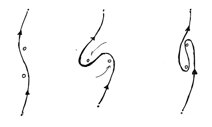
This explains that analytic continuation can only be ensured if we also avoid the set
The maps and are local diffeomorphisms thus, according to the above discussion, the following lemma finishes the proof.
Lemma 4.5.
If and are finite subsets of , the sum map induces a locally trivial fibration
Proof.
For the reader’s convenience, we include a proof of this elementary lemma. Denote by the minimal distance between the points and let be the bump function such that
Denote by tubular neighbourhoods of size and put . The restriction of the sum map above the complement of retracts by deformation on the complement over .
For a complex number , we use the subscript for its real part and for its imaginary part. Denote the horizontal and vertical distance by , for . Then, we put
Consider the vector fields
Near , we have , while near , we get that . Away from these sets we have and the vector field lifts . For and , we have
thus the vector fields commute and hence define a local trivialisation of the bundle. This proves the lemma and concludes the proof of the proposition. ∎
∎
Generalisation to higher dimensions
The -product which appears in the -product of , with , and determined by (9), is related to additive convolution by the formula:
| (12) |
Notice that the variables can be considered as a parameter . We may adapt Proposition 4.4 to this situation:
Proposition 4.6.
If are algebro-resurgent functions then the product is also algebro-resurgent.
Proof.
The set
is an algebraic variety of , . Thus, one can find a Zariski open subset over which the map
defines a locally trivial fibration. On each fibre of this fibration, one can repeat the proof of the one variable case. This proves the proposition. ∎
A closed formula for hypergeometric functions.
Contrary to the -product, the dual -product defines a non-commutative algebra for analytic power series (Proposition 2.2). According to Theorem 4.2, algebro-resurgent power series form a -subalgebra of functions having endless analytic continuation. The following proposition shows that algebraic functions do not form a -subalgebra :
Proposition 4.7.
The hypergeometric function
satisfies the identity
Proof.
Although this is expected by the description of the singularities of the -product, we prove the result directly by a naive direct computation.
First, note that if and do not depend on , then the -product reduces to the ordinary product: . In the case of one degree of freedom (, we get
Hence we see that the product of two elements that do not depend on is just equal to a certain Hadamard product [17]. Then,
After expanding the powers with the binomial theorem we see that the integral picks out corresponding -powers and we get
This proves the proposition. ∎
In particular, there might exist many closed formulærelating modular functions to -products. For instance, if we take then
which is exactly the elliptic modular function , for , with
5. Outlook.
Thanks to an integral formula proved in Proposition 3.3 for the -product, we have been able to continue analytically this product. Indeed, we introduced the notion of algebro-resurgence in Definition 4.1 and we proved that the set of all algebro-resurgent germs forms an algebra under the -product in Theorem 4.2. Note that we obtain as a byproduct that the class of Gevrey series in -variable which is Borel dual to the algebro-resurgent germs is an algebra for the -product, and it contains in particular the Euler series. Exponential small quantities - which encode interesting quantum effects - can be seen for example as the difference between the two Euler functions involved in (5), which admit both the Euler series as asymptotic series. In a Borel dual point a view, these exponential small quantities should be interpreted in terms of the singularities of functions in , which is one of the main ideas in resurgence theory.
As a particular case of algebro-resurgence, any -product of algebraic power series in (that is, elements from the Henselian local ring) is algebro-resurgent. In fact, algebraic power series are even holonomic, meaning that they satisfy a holonomic system of differential equations and the subset of holonomic power series happens to be closed under the -product. This is partly a consequence of the integral formula of Proposition 3.3: the stability under integration follows from the fact that integrals of vanishing cycles always satisfy a Picard-Fuchs type equation. The stability under the convolution of functions satisfying a linear differential equation is a classical theorem of Hurwitz. Details will appear elsewhere.
The algebra we have constructed here seems to be rich enough to capture interesting quantum effects. One of the main difficulties in Pham’s approach to Voros-Zinn-Justin conjectures was indeed the absence of a convenient tool to describe singularities arising from algebraic operations. As we saw here, the singularities of a star-product can be explicitly described in the Borel plane. This led to the observation that starting from certain algebraic functions, one ends up with hypergeometric functions (see Proposition 4.7). On one side, this shows that the star-product immediately produces highly transcendental functions but from the point of view of singularities, they stay relatively simple since hypergeometric functions are just solutions to linear differential equations with a finite number of poles.
In this paper, we gave an abstract description of singularities and apply it only on the simple example of hypergeometric functions. However, we expect that for the case of the anharmonic oscillator, we should be able to obtain an explicit description of the singularities such as conjectured by Delabaere-Pham [9] although these might involve complicated special functions.
There are also bigger algebras one could consider. Actually, the -exponential maps the algebra to a bigger one, and there are several ways in which one could try to enlarge so that the exponential maps the algebra to itself. Pham and coworkers define a subspace of resurgent germs in one variable, by saying that if for all there is a finite set , such that all can be analytically continued along all paths length that avoid [22]. In [7], the authors sketch an argument that is closed under convolution, and it would be tempting to try to construct an analogue quantum -algebra of this convolution algebra, using the integral formula of Proposition 3.3. However, as observed by Delabaere, Ou and Sauzin, there are some imprecisions in the original proofs of the convolution theorem for resurgent germs [20, 25]. We can see that the statement is true, by Proposition 4.4, if the singularity set is finite. Note that in the case the singularity set is a semi-group, detailed proofs have been given by Ou for one-dimensional semi-groups and by Sauzin in the two dimensional case.
Acknowledgments:
A. de Goursac acknowledges the F.R.S.-FNRS for financial support as well as the Belgian Interuniversity Attraction Pole (IAP) for support within the framework “Dynamics, Geometry and Statistical Physics” (DYGEST). M. Garay and A. de Goursac also acknowledge the Max Planck Institut für Mathematik in Bonn for invitation during this work.
References
- [1] F. Bayen, M. Flato, C. Fronsdal, A. Lichnerowicz, and D. Sternheimer, Deformation theory and quantization. I. Deformations of symplectic structures., Ann. Physics 111 (1978), no. 1, 61–110.
- [2] P. Bieliavsky and V. Gayral, Deformation Quantization for Actions of Kählerian Lie Groups, preprint arXiv:1109.3419 (2013), To appear in Mem. Amer. Math. Soc.
- [3] G.D. Birkhoff, Quantum mechanics and asymptotic series, Bulletin of the American Mathematical Society 39 (1933), no. 10, 681–700.
- [4] É. Borel, Leçons sur les séries divergentes, vol. 2, Gauthier-Villars, 1901.
- [5] M. Born and P. Jordan, Zur Quantenmechanik, Zeit. für Phys. 34 (1925), 858–888.
- [6] L. Boutet de Monvel and P. Krée, Pseudo differential operators and Gevrey classes, Annales de l’Institut Fourier 17 (1967), no. 1, 295–323.
- [7] B. Candelpergher, J.C. Nosmas, and F. Pham, Approche de la résurgence, Hermann, 1993, 289 pp.
- [8] Boris Chabat, Introduction à l’analyse complexe, tome II, Mir, 1976.
- [9] E. Delabaere and F. Pham, Unfolding the quartic oscillator, Annals of Physics 261 (1997), no. 2, 180–218.
- [10] M. Dimassi and J. Sjöstrand, Spectral asymptotics in the semi-classical limit, Lecture Note Series, no. 268, Cambridge University Press, 1999.
- [11] J. Écalle, Les fonctions résurgentes, vol. 1, algèbres de fonctions résurgentes, Pub. Math. Orsay (1981).
- [12] A. Eremenko, Geometric theory of meromorphic functions, Contemporary Mathematics 355 (2004), 221–230.
- [13] A. Eremenko and A. Gabrielov, Analytic continuation of eigenvalues of a quartic oscillator, Comm. Math. Physics 287 (2009), 431–457.
- [14] L. Euler, De seriebus divergentibus, Novi Commentarii academiae scientiarum Petropolitanae 5 (1760), 205–237, German translation available on http://www.eulerarchive.org/, E247.
- [15] M.D. Garay, Perturbative expansions in quantum mechanics, Annales de l’institut Fourier 59 (2009), no. 5, 2061–2101.
- [16] W. Gross, Eine ganze Funktion, für die jede komplexe Zahl Konvergenzwert ist, Mathematische Annalen 79 (1918), no. 1, 201–208.
- [17] J. Hadamard, Théorème sur les séries entières, Acta Mathematica 22 (1899), no. 1, 55–63.
- [18] A. Hurwitz, Sur une théorème de M. Hadamard, Comptes Rendus à l’Académie des Sciences 128 (1899), 350–353.
- [19] J. E. Moyal, Quantum mechanics as a statistical theory, Proc. Cambridge Philos. Soc. 45 (1949), 99–124.
- [20] Y. Ou, On the stability by convolution product of a resurgent algebra, Annales de la faculté des sciences de Toulouse Mathématiques 19 (2010), no. 3-4, 687–705.
- [21] F. Pham, Resurgence, quantized canonical transformations, and multi-instanton expansions, Algebraic analysis (M. Kashiwara and T. Kawai, eds.), vol. II, Academic Press, Boston, MA, 1988, Papers dedicated to Professor Mikio Sato on the occasion of his sixtieth birthday, pp. 699–726.
- [22] by same author, Multiple turning points in exact WKB analysis (variations on a theme of Stokes), Towards the exact WKB analysis of differential equations, linear or non linear (C. Howls, T. Kawai, and Y. Takei, eds.), Kyoto University Press, 2000, pp. 71–85.
- [23] M. Reed and B. Simon, Methods of modern mathematical physics, vol. IV, Academic Press, 1978.
- [24] M. A. Rieffel, Deformation Quantization for actions of R(D), Memoirs of the American Mathematical Society 106 (1993), R6.
- [25] D. Sauzin, On the stability under convolution of resurgent functions, arXiv:1201.1073, 2012.
- [26] J. Sjöstrand, Singularités analytiques microlocales, Astérisque 95 (1982), 1–166.
- [27] J.-L. Verdier, Stratifications de Whitney et théorème de Bertini-Sard, Inventiones Mathematicae 36 (1976), 295–312.
- [28] A. Voros, The return of the quartic oscillator (the complex WKB method), Ann. Inst. H. Poincaré, Phys. Théo. 39 (1983), 211–338.
- [29] J. Zinn-Justin, Multi-instanton contributions in quantum mechanics, 2, Nucl.Phys.B 218 (1983), 333–348.
- [30] J. Zinn-Justin and U. D. Jentschura, Multi-instantons and exact results I: conjectures, WKB expansions, and instanton interactions, Annals of Physics 313 (2004), no. 1, 197–267.
- [31] M. Zworski, Semiclassical analysis, vol. 138, AMS Bookstore, 2012.
Mauricio Garay
On leave from
Institut für Mathematik, FB 08 Physik, Mathematik und Informatik,
Johannes Gutenberg-Universität
55099 Mainz, Germany
garay91@gmail.com
Axel de Goursac
Chargé de Recherche au F.R.S.-FNRS,
IRMP, Université Catholique de Louvain,
Chemin du Cyclotron, 2, B-1348 Louvain-la-Neuve, Belgium
Axelmg@melix.net
Duco van Straten
Institut für Mathematik, FB 08 Physik, Mathematik und Informatik,
Johannes Gutenberg-Universität
55099 Mainz, Germany
straten@mathematik.uni-mainz.de