Theory and learning protocols for the material tempotron model

We studied the device described above within the replica theory, in a replica symmetric (RS) setting for the internal representations, in the limit of large $K$, both for the case in which $J_{i}\in\left\{-1,+1\right\}$ and $J_{i}\in\left\{0,1\right\}$, and estimated the entropy, the critical capacity, the optimal value for the threshold, and studied the structure of the space of the solutions and the valid internal representations. The results are almost identical for both $\pm 1$ and $0/1$ cases, so in the following we will only specify the model when a difference arises. We confirmed the results, where possible, with the cavity method (see section II.2). All details of the calculations are provided in the Appendix (section V); here we summarize the results.

The zero-temperature entropy of the device is defined as $S\left(\alpha\right)=\frac{1}{N}\left<\log\left(\mathcal{V}\right)\right>$, where $\mathcal{V}$ is the number of solutions (valid configurations of $J$’s) to the problem associated with some choice of the patterns $\xi_{it}^{\mu}$ and their expected outputs $s_{\textrm{exp}}^{\mu}$ (see also eq. 15), and $\left<\cdot\right>$ denotes the average over the patterns. $S\left(\alpha\right)$ can’t be negative (since the number of valid configurations is an integer number); the value of $\alpha$ at which $S\left(\alpha\right)$ vanishes is called the critical capacity, and represents the typical number of patterns per synapse which can be correctly classified by the device (i.e. stored) when the patterns are extracted according to the random i.i.d. distribution which we are studying.

The RS replica calculation predicts $S\left(\alpha\right)=\log\left(2\right)\left(1-\alpha\right)$, which interestingly does not depend on $K$ (provided $K\gg 1$). This function goes to zero at $\alpha_{c}=1$, which coincides with the information theoretic upper bound, i.e. the device is able to store one bit of information per synapse. This is in contrast with other related architectures, e.g. the multi-layer perceptron. After this point, the entropy is negative, and therefore the RS solution is no longer valid.

The typical value of the overlap between two different solutions to the same classification problem, defined as $q=\frac{1}{N}\left<\sum_{i=1}^{N}J_{i}^{a}J_{i}^{b}\right>$ for two solutions $\left\{J_{i}^{a}\right\}_{i\in\left\{1,\dots,N\right\}}$ and $\left\{J_{i}^{b}\right\}_{i\in\left\{1,\dots,N\right\}}$, is constant for all values of $\alpha$, and as low as possible, i.e. $q=0$ in the $\pm 1$ case and $q=Q^{2}=\nicefrac{{1}}{{4}}$ in the $0/1$ case, where $Q$ is the typical fraction of non-null synapses (which we found to be $Q=\nicefrac{{1}}{{2}}$). In terms of the structure of the space of the solutions, this means that the clusters of solutions are isolated (point-like).

We expand the threshold in series of $\sqrt{N}$ and write $\theta=\theta_{0}N+\theta_{1}\sqrt{N}$. The optimal value of $\theta_{0}$ is $0$ in the $\pm 1$ case and $\frac{f}{2}$ for the $0/1$ case; the value of $\theta_{1}$ does not affect the capacity, but we can set it so that synaptic values are unbiased:

$$\theta_{1}=-\sqrt{2f\left(1-f\right)}\textrm{erfc}^{-1}\left(2\sqrt[K]{1-f^{\prime}}\right)$$

(1)

where $\textrm{erfc}^{-1}$ is the inverse of the complementary error function.

We found that the valid internal representations follow a binomial distribution at large $K$, i.e. that the probability distribution for the value at each time bin is independent of the others. This fact is in agreement with the continuous model findings [6], and it is interesting for two reasons: on one hand, it confirms that different time bins are uncorrelated in the sparse limit, which is important in order to achieve efficiency in applying the cavity method. On the other hand, it means that the distributions of the input and output spike trains are identical (note that our choice of $f$ only ensures that the all-zero string occur with the same probability in input and output, but does not imply that the non-zero strings have the same distribution of the number of spikes). In turn, this is a necessary condition for recurrent networks to be built and work under this regime, which would be an interesting direction for future research.

We also computed how the internal representations are partitioned, and found that the rescaled entropy of the dominant internal representations (i.e. the logarithm of the number of different internal representations for a pattern which are associated with the largest portions of the solution space) is given by $\log\left(2\right)\log\left(\frac{K}{\log\left(2\right)}\right)$. This means that, as $K$ increases, the number of valid dominant internal representations increases as $K^{M\,\log 2}$, while the number of synaptic states associated with each of them correspondingly shrinks, so that the overall entropy remains constant.

The cavity method has been shown [10] to provide an alternative scheme for deriving the results from replica theory in the case of the binary perceptron with binary $\pm 1$ inputs and binary $\pm 1$ synapses. It has also been used on single instances of the learning problem on such devices (in which case it is known as the Belief Propagation algorithm, i.e. BP) to study the space of the solutions for some particular instance and for deriving heuristic learning algorithms [7, 8]. In those studies, the problem is represented as a factor graph in which synaptic weights are represented by variable nodes, and input patterns (and their desired outputs) are represented by factor nodes; messages are exchanged between the two types of nodes along the edges of the graph, representing marginal probabilities over the states of the variables; global thermodinamic quantities such as the entropy can be computed from the messages provided they satisfy the BP equations (which is typically achieved by reaching a fixed point in an iterative algorithm). Replica theory results can then be reproduced numerically with BP by averaging the computed quantities from a large number of samples of sufficient size.

In the case of the present study, however, in which the input patterns take values in $\left\{0,1\right\}$, the approach used in [7] can not be applied directly for the sake of reproducing replica theory results, not even in the perceptron limit $K=1$. This is due to a violation of the underlying assumption of the cavity method, known as the clustering property, as will be explained in greater detail at the end of this section, and as a result the standard BP equations are approximate, rather than becoming asymptotically exact in the large $N$ regime. Thus, in order to reproduce the replica theory results, the standard BP equations must be amended; however, since the heuristic algorithm described in section III.1 is based on the standard BP, which is simpler and more computationally efficient, and proves equally effective to the corrected-BP version, we will first derive the standard BP equations, and describe how to correct them afterwards.

Belief propagation equations, in their message passing form over single problem instances, have repeatedly proven to provide very effective heuristics when modified in order to produce optimal configurations [11, 8, 12]. Two main ways in which this can be achieved are decimation [13, 14] and reinforcement [7], which can be seen as a “soft decimation” process. In decimation, cycles are performed which alternate message passing and fixing (or “freezing”, or “decimating”) the most polarized free variables, until all variables are fixed. In reinforcement, the iterative equations have an additional term which has the role of a time-dependent external field, and which is computed from the magnetizations obtained at the preceding time step, so that the system is driven towards a completely polarized state. Following [7] the reinforced BP equations are the same as the normal BP equations with one single difference for eq. 2, which becomes:

$$m_{i\to\mu}^{\tau+1}=\tanh\left(\gamma\left(\tau\right)\tanh^{-1}\left(m_{i}^{\tau}\right)+\sum_{\nu\neq\mu}\tanh^{-1}\left(n_{\nu\to i}^{\tau+1}\right)\right)$$

(14)

where $\tau$ is the iteration step, $m_{i}^{\tau}=\tanh\left(\sum_{\nu}\tanh^{-1}\left(n_{\nu\to i}^{\tau}\right)\right)$ is the total magnetization of variable $i$ at iteration $\tau$, and $\gamma\left(\tau\right)$ is an iteration-dependent reinforcement parameter, which we set as $\gamma\left(\tau\right)=\gamma_{0}\tau$. Note that the additional term is proportional to the iteration step, and therefore dominates for large $\tau$, ensuring that polarization towards one single configuration is eventually achieved (although in practice computational problems will arise in difficult or unsatisfiable situations, due to the limited precision of the floating point representation).

We implemented both the decimation and the reinforcement schemes, for both the standard version of BP (for which the marginals are approximate due to correlations between different messages) and the corrected version (for which marginals are exact, at the cost of increased computational complexity and running time). Since we did not find the corrected version to provide any significant advantage over the naïve version (which is not particularly surprising, considering that the approximation provided by standard BP is rather good, and that the introduction of the reinforcement term introduces spurious correlations by itself), here we will only present results for the latter case.

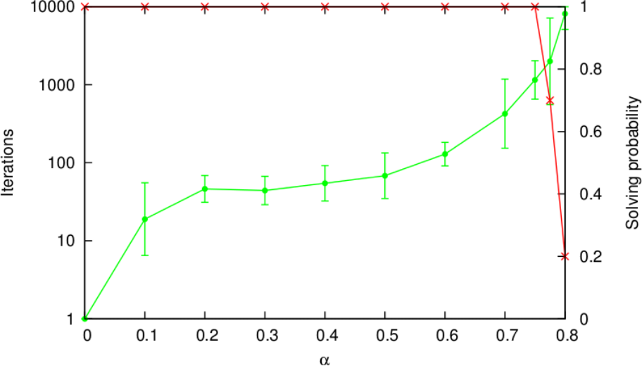
The value of $\gamma_{0}$ is a parameter of the solver algorithm; higher values of $\gamma_{0}$ make the algorithm greedier, in that the messages are polarized more quickly but can get trapped into a non-zero-energy state, while reducing $\gamma_{0}$ improves the accuracy of the algorithm at the cost of requiring more iterations. In practical tests, we found that by using eq. 5 we were able to reach values of $\alpha$ as high as $0.7$, but only at the cost of using extremely small values of $\gamma_{0}$ (of the order of $10^{-7}$ for $N=1000$ and $K=10$), and therefore of an impractically high computational time.

However, we found heuristically that, by detecting when an excessively polarized state was reached, and introducing a “depolarization event” triggered by such condition, we could achieve the same results with much higher values of $\gamma_{0}$, and therefore in a much shorter computational time. More in detail, we introduced, at each iteration step, a check to detect cases in which any of the terms in the denominator if eq. 5 goes to $0$, indicating a numerical problem due to excessively polarized magnetizations in a state of non-zero energy. Whenever this condition is found, we divide all messages $m_{i\to\mu}^{\tau}$ and total magnetizations $m_{i}^{\tau}$ by a positive factor $b$ (thus depolarizing all the messages), and reset $\gamma\left(\tau\right)$ to $0$. In subsequent iterations, we keep increasing $\gamma\left(\tau\right)$ linearly in steps of $\gamma_{0}$ (until another event is detected). We obtain good results by setting the factor $b$ to $2$ initially, and increasing it by one at every invocation of this additional depolarization rule. Indeed, since $\gamma\left(\tau\right)$ does not increase monotonically any more in this scheme, this modified algorithm will not be guaranteed to polarize towards a single state, unless the state itself has zero energy and therefore represents a solution to the problem.

Fig. 2 shows the performance of this algorithm for $N=1000$ and $K=10$. Setting $10000$ as the maximum number of iterations, a critical capacity of almost $0.8$ is achieved.

As for the case of the simple perceptron [7, 8, 9], it is possible to drastically simplify the reinforced BP equations (in a purely heuristic way), and obtain an online algorithm which, when parameters are set to their optimal values, proves to be almost as effective at learning as reinforced BP itself, while dramatically reducing computational requirements.

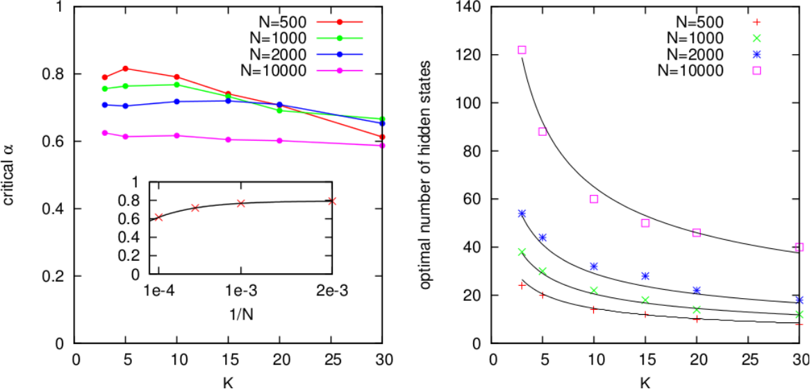
This algorithm requires a hidden state $h_{i}$ to be endowed with each synapse. This hidden state can only assume odd integer values, and is capped by a maximum absolute value $h^{\max}$, so that each synapse has a total of $h^{\max}+1$ hidden states. The hidden state and the synaptic weight $J_{i}$ are related by the simple expression $J_{i}=\textrm{sign}\left(h_{i}\right)$. In all simulations, we set the initial state of the $h_{i}$ states by randomly drawing values from $\left\{-1,1\right\}$.

The learning protocol turns out to be as follows: patterns $\xi^{\mu}$ are presented in random order to the device, computing the depolarization $\Delta_{t}^{\mu}=\left(\sum_{i=1}^{N}J_{i}\xi_{it}^{\mu}-\theta\right)$; from this, we determine $t^{\star}=\textrm{argmax}_{t}\Delta_{t}^{\mu}$ and compute $\Phi^{\mu}=\sigma_{\exp}^{\mu}\Delta_{t^{\star}}^{\mu}$; depending on the value of $\Phi^{\mu}$, we choose one of three actions:

$\Phi^{\mu}>1$

: do nothing

$0<\Phi^{\mu}\leq 1$

: with probability $r$, update synapses for which $\xi_{it^{\star}}^{\mu}=1$ and $J_{i}=\sigma_{\exp}^{\mu}$; with probability $\left(1-r\right)$ do nothing

$\Phi^{\mu}\leq 0$

: update all synapses for which $\xi_{it^{\star}}^{\mu}=1$

The synaptic update rule is always of this form:

$$h_{i}\to h_{i}+2\sigma_{\exp}^{\mu}$$

which implies that synaptic values $J_{i}$ are only updated in the $\Phi^{\mu}<0$ case, and only if $\xi_{it^{\star}}^{\mu}=1$ and $h_{i}=-\sigma_{\exp}^{\mu}$. As stated above, we impose $-h^{\max}\leq h_{i}\leq h^{\max}$, so that the update rule is not applied when $h_{i}=h^{\max}\sigma_{\exp}^{\mu}$.

The probability $r$ of taking an action in the “barely correct” case $0\leq\Phi^{\mu}\leq 1$ is a parameter of the algorithm, just as $h^{\max}$. We determined empirically the optimal values of $r$ and $h^{\max}$ for different values of $N$ and $K$ by extensively testing the space of the parameters. Our results, shown in fig. 3, indicate that $r=0.4$ works best for all values (we explored the values of $r$ in steps of $0.05)$, and that the optimal value of $h^{\max}$ is reasonably well fitted by a function $\lambda\sqrt{\nicefrac{{N}}{{K}}}$, where $\lambda=2.06\pm 0.02$. The capacity decreases with $N$, for fixed $K$, but does not seem to tend to $0$ asymptotically (see inset in fig. 3).

As a way to verify that the model and learning protocols which we studied are relevant in a more biologically realistic setting, we adapted the simplified BP-inspired scheme described in the previous section to address the continuous-time classification problem (see Introduction): for a given an instance of the problem, we discretize the time in $K$ bins, apply the BP-inspired learning protocol (slightly modified to use continuous inputs), and test the resulting synaptic weights assignments on the continuous device (see the Appendix for details, section VI). We found that in a device with $N=1000$ synapses, with time constants $t_{m}=10ms$ and $t_{s}=2.5ms$, tested on $T=500ms$ long input patterns discretized in $50$ bins, this scheme can achieve a classification error lower than 1% up to $\alpha=0.4$, demonstatrating that indeed under these conditions not much relevant information is typically lost in the time discretization process, and that the proposed time-discretized learning protocol can be effective even in a continuous-time setting.

We will consider the case in which synaptic weights take values in $\left\{-1,1\right\}$ first.

The volume of the space of the solutions for a given instantiation of the patterns can be written as:

$$\mathcal{V}=\sum_{\left\{J_{i}\right\}_{i}}\sum_{\left\{\tau_{t}^{\mu}\right\}_{\mu t}}\prod_{\mu}\chi\left(s_{\textrm{exp}}^{\mu},\left\{\tau_{t}^{\mu}\right\}_{t}\right)\prod_{\mu t}\Theta\left(\tau_{t}^{\mu}\left(\frac{1}{\sqrt{N}}\sum_{i}J_{i}\xi_{it}^{\mu}-\frac{\theta}{\sqrt{N}}\right)\right)$$

(15)

where index $i\in\left\{1,\dots,N\right\}$ is used for synapses, index $t\in\left\{1,\dots,K\right\}$ is used for time bins, index $\mu\in\left\{1,\dots,\alpha N\right\}$ is used for patterns, the auxiliary variables $\tau_{t}^{\mu}\in\left\{-1,1\right\}$ are the internal representations (they are equal to $2V_{t}^{\mu}-1$, see section I), and$\chi\left(s,\left\{\tau_{t}\right\}_{t}\right)=\Theta\left(s-\left(1-\prod_{t=1}^{K}\left(1-\frac{1}{2}\left(1+\tau_{t}^{\mu}\right)\right)\right)\right)$ is a characteristic function ensuring that the internal representation $\tau_{t}$ is compatible with the output $s$.

From here on, for simplicity, we will omit the subscript exp from the outputs $s^{\mu}$.

In order to compute the entropy, we need to compute the quenched average $\left\langle\log\mathcal{V}\right\rangle_{\xi,s}$; we do this by using the replica trick:[7, 8]

$$\left\langle\log\mathcal{V}\right\rangle_{\xi,s}=\lim_{n\to 0}\frac{\left\langle\mathcal{V}^{n}\right\rangle_{\xi,s}-1}{n}$$

(16)

where we compute $\left\langle\mathcal{V}^{n}\right\rangle_{\xi,s}$ for integer values of $n$, and use the analytic continuation to compute the limit $n\to 0$. The average over the replicated volume is:

$$\left\langle\mathcal{V}^{n}\right\rangle_{\xi,s}=\left\langle\sum_{\left\{J_{i}^{a}\right\}_{ia}}\sum_{\left\{\tau_{t}^{\mu a}\right\}_{\mu ta}}\prod_{\mu a}\chi\left(s^{\mu},\left\{\tau_{t}^{\mu a}\right\}_{t}\right)\prod_{\mu ta}\Theta\left(\tau_{t}^{\mu a}\left(\frac{1}{\sqrt{N}}\sum_{i}J_{i}^{a}\xi_{it}^{\mu}-\frac{\theta}{\sqrt{N}}\right)\right)\right\rangle_{\xi,s}$$

(17)

We used the index $a\in\left\{1,\dots,n\right\}$ to denote the replica. We can now use the integral representation of the $\Theta$ function, $\Theta\left(y\right)=\int_{-\infty}^{\infty}\frac{dx}{2\pi}\int_{0}^{\infty}d\lambda\,e^{ix\left(\lambda-y\right)}$, and compute the average over the input patterns, using their independence and the $N\gg 1$ limit (in the following, all integrals are assumed to be on $\left[-\infty,\infty\right]$ unless otherwise specified) :

	$\displaystyle\left\langle\prod_{a}\Theta\left(\tau_{t}^{\mu a}\left(\frac{1}{\sqrt{N}}\sum_{i}J_{i}^{a}\xi_{it}^{\mu}-\frac{\theta}{\sqrt{N}}\right)\right)\right\rangle_{\xi}=$		(18)
	$\displaystyle\quad=\int\prod_{a}\frac{dx_{t}^{\mu a}}{2\pi}\int_{0}^{\infty}\prod_{a}d\lambda_{t}^{\mu a}\,\prod_{a}\exp\left(ix_{t}^{\mu a}\left(\lambda_{t}^{\mu a}-\tau_{t}^{\mu a}\left(\bar{\xi}\frac{1}{\sqrt{N}}\sum_{i}J_{i}^{a}-\frac{\theta}{\sqrt{N}}\right)\right)\right)\cdot$
	$\displaystyle\quad\qquad\cdot\exp\left(-\frac{v_{\xi}}{2N}\sum_{a,b}\tau_{t}^{\mu a}\tau_{t}^{\mu b}x_{t}^{\mu a}x_{t}^{\mu b}\sum_{i}J_{i}^{a}J_{i}^{b}\right)$

where $\bar{\xi}=f$ and $v_{\xi}=f\left(1-f\right)$ are the average value and the variance of the inputs $\xi_{it}^{\mu}$, respectively. We then introduce order parameters $q^{ab}=\frac{1}{N}\sum_{i}J_{i}^{a}J_{i}^{b}$ and $T^{a}=-\sqrt{N}\bar{J}+\frac{1}{\sqrt{N}}\sum_{i}J_{i}^{a}$ via Dirac-delta functions, and their conjugates $\hat{q}^{ab}$,$\hat{T}^{a}$ via integral expansion of the deltas, and get:

	$\displaystyle\left\langle\mathcal{V}^{n}\right\rangle_{\xi,s}$	$\displaystyle=$	$\displaystyle\int\prod_{a}\frac{dT^{a}d\hat{T^{a}}\sqrt{N}}{2\pi}\int\prod_{a\geq b}\frac{dq^{ab}d\hat{q}^{ab}N}{2\pi}\exp\left(\sqrt{N}\sum_{a}\left(T^{a}+\sqrt{N}\bar{J}\right)\hat{T}^{a}-N\sum_{a\geq b}q^{ab}\hat{q}^{ab}\right)\cdot$		(19)
			$\displaystyle\cdot\left(\sum_{\left\{J_{i}^{a}\right\}_{ia}}\prod_{i}\exp\left(\sum_{a\geq b}\hat{q}^{ab}J_{i}^{a}J_{i}^{b}-\sum_{a}\hat{T}^{a}J_{i}^{a}\right)\right)\cdot$
			$\displaystyle\cdot\left\langle\sum_{\left\{\tau_{t}^{\mu a}\right\}_{\mu ta}}\prod_{\mu a}\chi\left(s^{\mu},\left\{\tau_{t}^{\mu a}\right\}_{t}\right)\right.\cdot$
			$\displaystyle\quad\cdot\prod_{\mu t}\left(\int\prod_{a}\frac{dx_{t}^{\mu a}}{2\pi}\int_{0}^{\infty}\prod_{a}d\lambda_{t}^{\mu a}\,\prod_{a}\exp\left(ix_{t}^{\mu a}\left(\lambda_{t}^{\mu a}-\tau_{t}^{\mu a}\left(\bar{\xi}\left(T^{a}+\sqrt{N}\bar{J}\right)-\frac{\theta}{\sqrt{N}}\right)\right)\right)\right.\cdot$
			$\displaystyle\quad\left.\left.\cdot\exp\left(-\frac{v_{\xi}}{2}\sum_{a,b}\tau_{t}^{\mu a}\tau_{t}^{\mu b}x_{t}^{\mu a}x_{t}^{\mu b}q^{ab}\right)\right)\right\rangle_{s}$
		$\displaystyle=$	$\displaystyle\int\prod_{a}\frac{dT^{a}d\hat{T^{a}}\sqrt{N}}{2\pi}\int\prod_{a\geq b}\frac{dq^{ab}d\hat{q}^{ab}N}{2\pi}\exp\left(\sqrt{N}\sum_{a}\left(T^{a}+\sqrt{N}\bar{J}\right)\hat{T}^{a}-N\sum_{a\geq b}q^{ab}\hat{q}^{ab}\right)\cdot$
			$\displaystyle\cdot\left(\sum_{\left\{J^{a}\right\}_{a}}\exp\left(\sum_{a\geq b}\hat{q}^{ab}J^{a}J^{b}-\sum_{a}\hat{T}^{a}J^{a}\right)\right)^{N}\cdot$
			$\displaystyle\cdot\left\langle\sum_{\left\{\tau_{t}^{a}\right\}_{ta}}\prod_{a}\chi\left(s,\left\{\tau_{t}^{a}\right\}_{t}\right)\right.\cdot$
			$\displaystyle\quad\cdot\prod_{t}\left(\int\prod_{a}\frac{dx_{t}^{a}}{2\pi}\int_{0}^{\infty}\prod_{a}d\lambda_{t}^{a}\,\prod_{a}\exp\left(ix_{t}^{a}\left(\lambda_{t}^{a}-\tau_{t}^{a}\left(\bar{\xi}\left(T^{a}+\sqrt{N}\bar{J}\right)-\frac{\theta}{\sqrt{N}}\right)\right)\right)\right.\cdot$
			$\displaystyle\quad\left.\left.\cdot\exp\left(-\frac{v_{\xi}}{2}\sum_{a,b}\tau_{t}^{a}\tau_{t}^{b}x_{t}^{a}x_{t}^{b}q^{ab}\right)\right)\right\rangle_{s}^{\alpha N}$

where in the second step we dropped indices $i$ and $\mu$. We expand the threshold $\theta$ in series of $\sqrt{N}$:

$$\theta=N\theta_{0}+\sqrt{N}\theta_{1}$$

(20)

from which we immediately get the relation:

$$\bar{J}=\frac{\theta_{0}}{\bar{\xi}}$$

(21)

This leaves us with:

	$\displaystyle\left\langle\mathcal{V}^{n}\right\rangle_{\xi,s}$	$\displaystyle=$	$\displaystyle\int\prod_{a}\frac{dT^{a}d\hat{T^{a}}\sqrt{N}}{2\pi}\int\prod_{a\geq b}\frac{dq^{ab}d\hat{q}^{ab}N}{2\pi}\cdot$		(22)
			$\displaystyle\cdot\exp\left(\sqrt{N}\sum_{a}T^{a}\hat{T}^{a}+N\bar{J}\sum_{a}\hat{T}^{a}-N\sum_{a\geq b}q^{ab}\hat{q}^{ab}\right)\cdot$
			$\displaystyle\cdot\left(\sum_{\left\{J^{a}\right\}_{a}}\exp\left(\sum_{a\geq b}\hat{q}^{ab}J^{a}J^{b}-\sum_{a}\hat{T}^{a}J^{a}\right)\right)^{N}\cdot$
			$\displaystyle\cdot\left\langle\sum_{\left\{\tau_{t}^{a}\right\}_{ta}}\prod_{a}\chi\left(s,\left\{\tau_{t}^{a}\right\}_{t}\right)\prod_{t}\left(\int\prod_{a}\frac{dx_{t}^{a}}{2\pi}\int_{0}^{\infty}\prod_{a}d\lambda_{t}^{a}\,\prod_{a}\exp\left(ix_{t}^{a}\left(\lambda_{t}^{a}-\tau_{t}^{a}\left(\bar{\xi}T^{a}-\theta_{1}\right)\right)\right)\right.\right.\cdot$
			$\displaystyle\quad\left.\left.\cdot\exp\left(-\frac{v_{\xi}}{2}\sum_{a,b}\tau_{t}^{a}\tau_{t}^{b}x_{t}^{a}x_{t}^{b}q^{ab}\right)\right)\right\rangle_{s}^{\alpha N}$

In the $N\gg 1$ limit, this integral can be computed by the saddle point method: we introduce the RS Ansatz for the solution: $T^{a}=T\,\forall a$, $q^{ab}=q\,\forall a,b:a\neq b$, $q^{aa}=Q\,\forall a$, and analogous expressions for the conjugate parameters. Therefore:

	$\displaystyle\left\langle\mathcal{V}^{n}\right\rangle_{\xi,s}$	$\displaystyle=$	$\displaystyle\exp\left(N\bar{J}\hat{T}+N\frac{n}{2}\hat{q}q-Nn\hat{Q}Q\right)\cdot$		(23)
			$\displaystyle\cdot\left(\sum_{\left\{J^{a}\right\}_{a}}\exp\left(\frac{\hat{q}}{2}\left(\sum_{a}J^{a}\right)^{2}-\frac{1}{2}\left(\hat{q}-2\hat{Q}\right)\sum_{a}\left(J^{a}\right)^{2}-\hat{T}\sum_{a}J^{a}\right)\right)^{N}\cdot$
			$\displaystyle\cdot\left\langle\sum_{\left\{\tau_{t}^{a}\right\}_{ta}}\prod_{a}\chi\left(s,\left\{\tau_{t}^{a}\right\}_{t}\right)\prod_{t}\left(\int\prod_{a}\frac{dx_{t}^{a}}{2\pi}\int_{0}^{\infty}\prod_{a}d\lambda_{t}^{a}\,\prod_{a}\exp\left(ix_{t}^{a}\left(\lambda_{t}^{a}-\tau_{t}^{a}\left(\bar{\xi}T-\theta_{1}\right)\right)\right)\right.\right.\cdot$
			$\displaystyle\quad\left.\left.\cdot\exp\left(-\frac{v_{\xi}}{2}\left(q\left(\sum_{a}\tau_{t}^{a}x_{t}^{a}\right)^{2}+\left(Q-q\right)\sum_{a}\left(x_{t}^{a}\right)^{2}\right)\right)\right)\right\rangle_{s}^{\alpha N}$
		$\displaystyle=$	$\displaystyle\exp\left(N\bar{J}\hat{T}+N\frac{n}{2}\hat{q}q-Nn\hat{Q}Q\right)\cdot$
			$\displaystyle\cdot\left(\int Du\left(\sum_{\left\{J\right\}}\exp\left(-\frac{1}{2}\left(\hat{q}-2\hat{Q}\right)J^{2}+\left(\sqrt{\hat{q}}u-\hat{T}\right)J\right)\right)^{n}\right)^{N}\cdot$
			$\displaystyle\cdot\left(\int\prod_{t}Du_{t}\left\langle\left(\sum_{\left\{\tau_{t}\right\}_{t}}\chi\left(s,\left\{\tau_{t}\right\}_{t}\right)\prod_{t}\left(\int\frac{dx_{t}}{2\pi}\int_{0}^{\infty}d\lambda_{t}\,\exp\left(-\frac{v_{\xi}}{2}\left(Q-q\right)\left(x_{t}\right)^{2}\right)\right.\right.\right.\right.\cdot$
			$\displaystyle\quad\left.\left.\left.\left.\cdot\exp\left(ix_{t}\left(\lambda_{t}-\tau_{t}\left(\bar{\xi}T-\theta_{1}-\sqrt{v_{\xi}q}u_{t}\right)\right)\right)\right)\right)^{n}\right\rangle_{s}\right)^{\alpha N}$
		$\displaystyle=$	$\displaystyle\exp\,Nn\left(\bar{J}\hat{T}+\frac{1}{2}\hat{q}q-\hat{Q}Q\right.+$
			$\displaystyle\qquad+\int Du\,\log\left(\sum_{\left\{J\right\}}\exp\left(-\frac{1}{2}\left(\hat{q}-2\hat{Q}\right)J^{2}+\left(\sqrt{\hat{q}}u-\hat{T}\right)J\right)\right)$
			$\displaystyle\qquad+\left.\alpha\int\prod_{t}Du_{t}\left\langle\log\left(\sum_{\left\{\tau_{t}\right\}_{t}}\chi\left(s,\left\{\tau_{t}\right\}_{t}\right)\prod_{t}H\left(-\tau_{t}\frac{\bar{\xi}T-\theta_{1}-\sqrt{v_{\xi}q}u_{t}}{\sqrt{v_{\xi}\left(Q-q\right)}}\right)\right)\right\rangle_{s}\right)$

where in the second step we introduced auxiliary Gaussian integrals (we use the shorthand notation $Du=du\frac{1}{\sqrt{2}\pi}e^{-\frac{u^{2}}{2}}$ and define $H\left(x\right)=\int_{x}^{\infty}\ Dy$), which allows to drop the replica index $a$, and in the last step we used the $n\to 0$ limit. Finally, we obtain the expression for the entropy:

	$\displaystyle\mathcal{S}=\frac{1}{N}\left\langle\log\mathcal{V}\right\rangle_{\xi,s}$	$\displaystyle=$	$\displaystyle\bar{J}\hat{T}+\frac{1}{2}\hat{q}q-\hat{Q}Q+\mathcal{Z}_{J}\left(\hat{Q},\hat{q},\hat{T}\right)+\mathcal{Z}_{S}\left(Q,q,T\right)$		(24)
	$\displaystyle\mathcal{Z}_{J}\left(\hat{Q},\hat{q},\hat{T}\right)$	$\displaystyle=$	$\displaystyle\int Du\,\log\left(\sum_{\left\{J\right\}}\exp\left(-\frac{1}{2}\left(\hat{q}-2\hat{Q}\right)J^{2}+\left(\sqrt{\hat{q}}u-\hat{T}\right)J\right)\right)$		(25)
	$\displaystyle\mathcal{Z}_{S}\left(Q,q,T\right)$	$\displaystyle=$	$\displaystyle\alpha\int\prod_{t}Du_{t}\left\langle\log\left(\sum_{\left\{\tau_{t}\right\}_{t}}\chi\left(s,\left\{\tau_{t}\right\}_{t}\right)\prod_{t}H\left(-\tau_{t}\,\eta\left(u_{t},Q,q,T\right)\right)\right)\right\rangle$		(26)
	$\displaystyle\eta\left(u,Q,q,T\right)$	$\displaystyle=$	$\displaystyle\frac{\bar{\xi}T-\theta_{1}-\sqrt{v_{\xi}q}u}{\sqrt{v_{\xi}\left(Q-q\right)}}$		(27)

The expression for $\mathcal{Z}_{J}$ is the familiar expression for perceptron models, and it can be written more explicitly for the two cases $J\in\left\{-1,1\right\}$ and $J\in\left\{0,1\right\}$:

	$\displaystyle\mathcal{Z}_{J}^{\pm}\left(\hat{Q},\hat{q},\hat{T}\right)$	$\displaystyle=$	$\displaystyle-\frac{1}{2}\left(\hat{q}-2\hat{Q}\right)+\int Du\,\log\left(2\cosh\left(\sqrt{\hat{q}}u-\hat{T}\right)\right)$		(28)
	$\displaystyle\mathcal{Z}_{J}^{01}\left(\hat{Q},\hat{q},\hat{T}\right)$	$\displaystyle=$	$\displaystyle\int Du\,\log\left(1+\exp\left(-\frac{1}{2}\left(\hat{q}-2\hat{Q}\right)+\sqrt{\hat{q}}u-\hat{T}\right)\right)$		(29)

References

- [1] Gütig R and Sompolinsky H 2006 Nature Neuroscience 9 420–428 ISSN 1097-6256 URL http://www.nature.com/neuro/journal/v9/n3/abs/nn1643.html
- [2] Johansson R S and Birznieks I 2004 Nature Neuroscience 7 170–177 ISSN 1097-6256 URL http://www.nature.com/neuro/journal/v7/n2/full/nn1177.html
- [3] deCharms R C and Merzenich M M 1996 Nature 381 610–613 ISSN 0028-0836
- [4] Meister M, Lagnado L and Baylor D A 1995 Science 270 1207–1210 ISSN 0036-8075
- [5] Wehr M and Laurent G 1996 Nature 384 162–166 ISSN 0028-0836
- [6] Rubin R, Monasson R and Sompolinsky H 2010 Physical Review Letters 105 218102 URL http://link.aps.org/doi/10.1103/PhysRevLett.105.218102
- [7] Braunstein A and Zecchina R 2006 Physical Review Letters 96 030201 URL http://prl.aps.org/abstract/PRL/v96/i3/e030201
- [8] Baldassi C, Braunstein A, Brunel N and Zecchina R 2007 Proceedings of the National Academy of Sciences 104 11079–11084 ISSN 0027-8424, 1091-6490 PMID: 17581884 URL http://www.pnas.org/content/104/26/11079
- [9] Baldassi C 2009 Journal of Statistical Physics 136 ISSN 0022-4715 (Print) 1572-9613 (Online) URL http://www.springerlink.com/content/r07772l167526045/
- [10] Mézard, M 1989 Journal of Physics A: Mathematical and General 22 2181–2190 ISSN 0305-4470, 1361-6447
- [11] Braunstein A, Kayhan F, Montorsi G and Zecchina R 2007 Encoding for the blackwell channel with reinforced belief propagation IEEE International Symposium on Information Theory (ISIT07) pp 1891–1895
- [12] Bailly-Bechet M, Borgs C, Braunstein A, Chayes J, Dagkessamanskaia A, François J and Zecchina R 2010 Proceedings of the National Academy of Sciences 108 882–887 ISSN 0027-8424 URL http://www.pnas.org/content/108/2/882.short
- [13] Mézard M, Parisi G and Zecchina R 2002 Science 297 812 – 815 ISSN 10959203
- [14] Braunstein A, Mézard M and Zecchina R 2005 Random Structures and Algorithms 27 201–226
- [15] Monasson R and Zecchina R 1996 Physical Review Letters 76 2205–2205 URL http://link.aps.org/doi/10.1103/PhysRevLett.76.2205.3
- [16] Cocco S, Monasson R and Zecchina R 1996 Physical Review E 54 717–736 URL http://link.aps.org/doi/10.1103/PhysRevE.54.717