Structural thermokinetic modelling
Abstract
Translating metabolic networks into dynamic models is difficult if kinetic constants are unknown. Structural Kinetic Modelling (SKM) starts from a given metabolic state, defined by metabolite concentrations and fluxes, and replaces the reaction elasticities in this state – the sensitivities of reaction rates to reactant concentrations – by independent random numbers. Here I propose a variant that accounts for reversible reactions and thermodynamics: in Structural Thermokinetic Modelling (STM), correlated elasticities are computed from enzyme saturation values and thermodynamic forces, which are physically independent. STM relies on a dependency schema in which basic variables can be sampled, fitted to data, or optimised, while all other variables are computed from them. Probability distributions in the dependency schema define a model ensemble, which leads to probabilistic predictions even if data are scarce. STM highlights the importance of variabilities, dependencies and covariances of biological variables. By choosing or sampling the basic variables, we can convert metabolic networks into kinetic models with consistent reversible rate laws. Metabolic control coefficients obtained from these models can tell us about metabolic dynamics, including responses and optimal adaptations to perturbations as well as enzyme synergies, metabolite correlations, and metabolic fluctuations arising from chemical noise. By comparing model variants with different network structures, fluxes, thermodynamic forces, regulation, or types of rate laws, we can quantify the effects of these model features. To showcase STM, I study metabolic control, metabolic fluctuations, and enzyme synergies, and how they are shaped by thermodynamic forces. Thermodynamics can be used to obtain more precise predictions of flux control, enzyme synergies, correlated flux and metabolite variations, and of the emergence and propagation of metabolic noise.
Keywords: Metabolic model, structural kinetic modelling, dependency schema, elasticity, ensemble model
Abbreviations: SKM: Structural kinetic modelling; MCT: Metabolic control theory; FBA: Flux balance analysis; MoMA: Minimization of metabolic adjustment.
1 Introduction
The metabolic fluxes in cells are shaped by network structure, reaction thermodynamics, enzymatic rate laws, and enzyme regulation. Flux, metabolite, and protein data provide a detailed picture of metabolism, and computational models can help us answer important questions. For example, how do enzyme-inhibiting drugs, enzyme overexpression, or changes in nutrient levels affect the cell’s metabolic states? Will local enzyme perturbations have long-range effects on the fluxes, or are they compensated by changes of nearby metabolite concentrations [1]? To address such questions, metabolic networks, comprising thousands of reactions, have been built [2, 3], and methods such as Flux Balance Analysis (FBA) [4, 5], MoMA [6], the principle of minimal fluxes [7], or ROOM [8] predict plausible flux distributions from heuristic assumptions [9] or sampling [10]. Thermodynamic flux analysis [11, 12, 13, 14] relates fluxes to metabolite concentrations via equilibrium constants and thermodynamic forces. However, it does not describe how metabolic fluxes arise mechanistically. How can we predict the effects of enzyme concentrations, external metabolite concentrations, or parameters like temperature or the dilution rate on fluxes? If metabolite concentrations were constant, reaction fluxes would be directly proportional to enzyme concentrations. But in reality this is different: the interplay between fluxes, concentrations, and enzyme activities leads to stationary fluxes and metabolite concentrations, which depend on enzyme levels in complicated ways. To understand how an enzyme inhibition changes metabolic fluxes, we need to consider its effect on metabolite concentrations. Flux analysis cannot describe this because rate laws, enzyme saturation, and regulation by effector molecules, are not even considered. Kinetic models would allow us to quantify the effects of enzyme perturbations (or other parameter perturbations) on fluxes and metabolite concentrations in steady state, but kinetic rate laws and rate constants are largely unknown, especially in less well-studied organisms.
Close to a steady state, metabolic dynamics can be described by linearised models. Metabolic Control Theory [15, 16] (MCT, Figure 1), considers local perturbations (for example enzyme inhibitions), quantifies their direct effect on reaction rates, and infers network-wide effects on the steady state. MCT uses two types of sensitivity coefficients: reaction elasticities describe how reaction rates change with changing metabolite concentrations: they concern immediate effects on a fast timescale (which depend only on rate laws of reactions perturbed). Response and control coefficients, which depend on network structure and elasticities, describe long-term, wide-range effects of parameter perturbations on steady-state fluxes and concentrations (see Supplementary Materials). MCT has various applications. Using response coefficients, we can assess the effects of enzyme inhibition, differential enzyme expression, varying external metabolite concentrations, enzyme inhibition by drugs, or genetic modifications. A Taylor expansion based on response coefficients can also describe more complicated perturbations (e.g. simultaneous activity changes of all enzymes), optimal enzyme allocation in pathways [17], and parameter uncertainty or variability [18]. Second-order response coefficients [19], describing synergy effects, play a role in predicting optimal differential expression [20]. In systems with periodic [21, 22] or random [18] parameter fluctuations, the fluctuations of fluxes and metabolite concentrations depend on spectral response coefficients. Importantly, all these phenomena can be described without a full kinetic model: linearised models with the same network structure and reaction elasticities as in the original model, suffices to describe the dynamics of small fluctuations caused by static or periodic parameter perturbations or chemical noise, and powerful theory exists for optimal control and model reduction in linear models [23]. So all we need to know are network structure and (first or second order) elasticities. But if only the network structure is known, how can we obtain elasticities from few or no other data?
Since elasticities are unknown (unless a kinetic model is already available), Structural Kinetic Modelling (SKM, [24, 25]), the ORACLE framework [26, 27, 28, 29], and similar methods [30, 31, 32, 33] replace them by random numbers. Reaction rates increase with the substrate concentrations and decrease with the product concentrations, and this is encoded in the signs of reaction elasticities: positive for substrates and activators, and negative for products and inhibitors (where “substrate” and “product”, in this case, refer to the flux direction). Assuming irreversible rate laws, SKM equates the scaled elasticities to saturation values, numbers between 0 and 1 that describe the fraction of catalysing enzyme molecules that are bound, on average, to metabolites. In SKM, saturation values are treated as free variables and sampled from random distributions. Possible bounds can be derived from the rate laws (e.g. the range for substrate elasticities in mass-action rate laws). The resulting elasticity matrix is sparse, reflecting network structure and regulation arrows. Each row describes one reaction: substrates and activators lead to positive matrix elements, while products and inhibitors lead to negative elements. To sample the elasticities, each non-zero matrix element is replaced by a random number with the required sign. Each sampled elasticity matrix defines a linearised kinetic model, whose Jacobian matrix determines the stability of the reference state as well as the dynamic behaviour around it. Given metabolite concentrations and fluxes, reaction elasticities can be converted into kinetic constants: hence, instead of sampling elasticities it is also possible to sample some kinetic parameters directly and to compute the others [34, 35]. Structural kinetic modelling has been applied to various cell biological questions [36, 37, 38, 39].
If elasticities are variable, uncertain, or unknown, how will this translate into (actual) variability or (or subjective) uncertainty? To explore this variability or uncertainty, we can study model ensembles in which some model features are given (e.g. network structure and flux distribution), while others are varied (e.g. metabolite concentrations and kinetic constants). By sampling variable model features from random distributions [18, 40] and translating the linearised model back into a full kinetic model, a model ensemble can be created. Given a set of sampled model instances, we can estimate the probability distributions for an infinitely large ensemble. In practice, by generating many model instances (each with its own elasticity matrix), one can explore the possible dynamics allowed by our network, and assess their probabilities. By computing probabilities for model outputs or types of behaviour, we can see how they depend on network structure, fluxes, or rate laws. If most of the model instances show a certain behaviour, this behaviour can be attributed to model structure (or generally: to features that were fixed during sampling), while varying properties may be attributed to the features sampled. In the model ensemble, we can also screen for models with a given property – e.g. stable oscillations – and check which model details (e.g. inhibition arrows or specific elasticity values) are overabundant in this subensemble, and thus potentially causing these features [24]. Finally, different model variants can be compared (e.g., with different network structures, regulation arrows, different fluxes, etc.): each model variant is translated into a model ensemble and significant differences between the ensembles can be attributed to differences in model structure.
Despite all its merits, ensemble modelling by SKM has one major drawback: it ignores the fact that elasticities are interdependent due to basic physical laws. The net flux in chemical reactions results from a difference of one-way rates and , the rates of microscopic reaction events in forward and backward direction. In chemical equilibrium states, the ratio of product and substrate concentrations is given by the equilibrium constant: the net rate vanishes and the two one-way rates must be equal. More generally, their ratio is given by with the dimensionless thermodynamic force , the reaction Gibbs free energy (given by the difference of chemical potentials along a reaction), Boltzmann’s gas constant , absolute temperature [41]. The quantity is called reaction affinity. Depending on their thermodynamic force (which depends on substrate and product concentrations), reactions range between two extremes. In equilibrium reactions, the force vanishes, the one-way rates and are equal, and the net flux vanishes. Strongly driven reactions, in contrast, have large thermodynamic forces, a negligible backward flux , and a net flux close to the forward flux . By tuning the one-way fluxes (), the thermodynamic force shapes elasticities: if a force is large, the backward rate will be negligible, the net rate is does not dependent on the product concentrations, and the product elasticities vanish. Since the forces themselves satisfy Wegscheider conditions (a zero sum over loops in the network) and elasticities are dependent on them, elasticities may be interdependent (and thus, correlated in reality) across the entire network [42]. Ignoring this fact, SKM leads to thermodynamically inconsistent models [42] (for an example, see Supplementary Materials).
How can we solve this problem? Sampling correlated elasticities – satisfying network-wide thermodynamic constraints – seems difficult, but it is actually easy for certain rate laws: using formulae from [42], elasticities can be computed from thermodynamic forces and saturation values, variables that can by independently varied. Below I use this to construct model ensembles: I describe an algorithm for sampling reaction elasticities, while fully accounting for dependencies due to reversible rate laws. I then show how thermodynamics and enzyme saturation shape control properties, dynamic timecourses, enzyme synergies, and fluctuations in metabolic systems. Importantly, also enzyme synergies and other second-order effects are described by closed formulae. Since it adds thermodynamics to SKM, the framework is called Structural Thermokinetic Modelling. Compared to the original SKM, modelling is more formalised: all model variables (including the reference metabolite concentrations and fluxes) are determined step by step, by inserting known values, sampling, or optimisation. A thermodynamically feasible metabolic state is a basis for constructing thermodynamically feasible models. The workflow follows a schema that describes the model variables, guarantees physical correctness, and can be used to define probability distributions. By separating network (defining the biological system) and schema (defining the types of variables and their physical dependencies), models can be build flexibly, and their mathematical relationships are easy to see. This makes STM particularly suitable for automatic model construction.
2 Materials and Methods
2.1 Constructing kinetic metabolic models
To build metabolic models, STM relies on kinetic and thermodynamic laws and on Metabolic Control Theory. An overview of concepts and formulae is given in Supplementary Materials. To translate metabolic networks into kinetic models, we need to integrate data about kinetics, thermodynamics, and metabolic states. In general, model construction poses a number of challenges: (i) finding realistic rate laws and kinetic constants; (ii) ensuring consistent equilibrium states of the model, with metabolite concentrations leading to vanishing fluxes; (iii) choosing a reference state with realistic fluxes and metabolite concentrations; and (iv) assessing variability and uncertainties in model parameters and metabolic states. Metabolic model can be parameterised automatically with the help of generic rate laws including mass-action, power-law [43], linlog [44], or modular rate laws [45, 42]. The use of reversible rate laws with consistent kinetic constants (satisfying Wegscheider conditions and Haldane relationships) can guarantee consistent equilibrium states.
In kinetic models, enzyme levels and external metabolite concentrations are usually treated as parameters that determine the steady state. However, such model are difficult to fit to fluxes (whether measured or predicted by FBA). Retromodelling reverts this procedure: we start from a flux distribution and construct metabolite concentrations and rate laws around it. We can do this as follows. After choosing the fluxes, the MDF method [46] can be used to find feasible metabolite concentrations and thermodynamic bottlenecks (reactions with inevitably poor thermodynamic forces). Then, there are different ways to proceed. First, one may define reversible rate laws, choose plausible metabolite concentrations, and compute the enzyme demands [47, 48, 34], or optimise metabolite and enzyme concentrations simultaneously for a minimal enzyme cost [49]. Second, one may first construct a full metabolic state (including fluxes and metabolic concentrations) and then find kinetic constants that can realise this state.
2.2 Elasticities and their dependence on thermodynamic forces
Enzyme kinetics, thermodynamic forces, and metabolic control are closely related (Figure 1). The metabolic dynamics close to a reference state depend on reaction elasticities, defined as derivatives of kinetic rate laws with respect to metabolite concentrations . At high substrate concentrations, an enzyme becomes saturated, and additional substrate has little effect, so the elasticity is low. Elasticities describe the immediate, local effects of metabolite perturbations on reaction rates: to define them, we formally assume that metabolite concentrations are not dynamic variables, but parameters to be tuned from the outside. Elasticities between rates and other variables, e.g. enzyme levels, are defined accordingly. Importantly, our (so-called unscaled) elasticities can be rewritten as with unitless scaled elasticities defined as (or ). Scaled elasticities describe effective reaction orders. For irreversible rate laws, we obtain in the linear range and near saturation. In general, indicates that two molecules of the same substrate are used. Formulae for second-order elasticities (defined via second derivatives) are given in Supplementary Materials. To linearise a metabolic model around a reference state, we just need the stoichiometric matrix and the unscaled elasticity matrix . Both matrices can easily be obtained if the reference state (metabolite levels and fluxes) is known. A perturbation (e.g. by an initial perturbation vector ) will lead to a linearised dynamics; by solving the differential equations with the Jacobian matrix we can simulate the propagation of dynamic perturbations across the network and determine their long-term effects [23]. In models with conserved moieties, a complication arises: if the internal stoichiometric matrix has non-full row rank, and we need to focus on independent metabolite concentrations. Their concentrations follow a dynamic equation with Jacobian matrix , and , where and has full row rank.
Enzyme elasticities are subject to multiple functional requirements. At low saturation (i.e. high elasticities), the enzyme efficiency (flux per enzyme level) is low, and the enzyme demand per flux (i.e. the inverse enzyme efficiency) is high. At high saturation, a different problem arises: the reaction rate hardly changes with the substrate level, so the reaction is “stiff”: fluctuations in inflowing substrate cannot be buffered and lead to large fluctuations in substrate levels. Hence, the optimal choice of elasticities (and thus, of saturation values) reflects trade-offs between enzyme demand and favourable control properties.

Modular rate laws (see Supplementary Materials) are generic reversible rate laws based on simple enzyme mechanisms, with random-order binding. The formulae contain terms of the form , called saturation values. A saturation value describes the saturation of an enzyme with a reactant or small-molecule regulator, where is a metabolite concentration, and is the dissociation constant between enzyme and metabolite (X stands for M (reactants), A (activators), or I (inhibitors)). In modular rate laws, which are based on a quasi-equilibrium approximation [42], the are dissociation constants and half-saturation concentrations at the same time. Saturation values range between 0 and 1, and from saturation values and metabolite concentrations, we can reconstruct the dissociation constants . The scaled elasticities of modular rate laws consist of two terms [42],
| (1) |
The thermodynamic “reversibility” term depends directly on the thermodynamic force . The kinetic term arises from kinetics and depends on the saturation values. Since forces are coupled through Wegscheider conditions, the elasticities must be interdependent. However, given the forces and metabolite concentrations, the saturation values can be freely varied without violating any physical laws (proof see Supplementary Materials). Details about modular rate laws and their (first- and second-order) elasticities can be found in [42].
All (thermodynamically consistent) reversible rate laws share the same numerator, which has the shape of mass-action rate law [42]. The numerator leads to the thermodynamic elasticity term [42]
| (2) |
with substrate and product molecularities and and a flux ratio . Coming back to Eq. (2), the flux ratio, and therefore the elasticity term depends on the thermodynamic force , with Boltzmann’s gas constant and absolute temperature . For forward reactions near equilibrium (i.e. small positive thermodynamic forces ), the substrate terms (where ) are close to infinity and the product terms (where ) are close to . For completely forward-driven reactions (with thermodynamic force ), we obtain elasticities (for substrates) and (for products). Between these extremes, the elasticities vary with the thermodynamic force. With a small force of 1 kJ/mol 0.4 RT (and molecularities and stoichometric coefficients equal to 1), Eq. (2) yields substrate elasticities of and product elasticities of . In contrast, for a force of 10 kJ/mol we obtain values of 1.02 (substrate) and -0.02 (product).
The form of the kinetic elasticity term depends on the type of modular rate law. With mass-action or power-law rate laws without regulation, the kinetic term vanishes and the elasticities follow directly from network structure and driving forces:
| (3) |
With other rate laws, a kinetic elasticity term needs to be added. For example, for the simultaneous-binding modular (SM) rate law with non-competitive activation and inhibition [42], the kinetic term consists of four terms (related to substrates S, products P, activators A, and inhibitors I):
| (4) |
The two terms reflect two parts of the rate law: a prefactor for regulation and the rate law denominator. Eq. (4) generalises Structural Kinetic Modelling: the elasticity formula in SKM,
| (5) |
is a limiting case of Eq. (4) for completely forward-driven reactions, where and . For reversible reactions, a difference remains: in contrast to SKM, the thermodynamic term in STM makes elasticities thermodynamically consistent and interdependent. With the common modular rate law [42] (or “convenience kinetics” [45]), the formula for scaled elasticities is more complicated:
| (6) |
where . Formulae for other rate laws and second-order elasticities can be found in [42] and Supplementary Materials.
There is another useful elasticiy formula. If the flux directions are known, reversible rate laws can be written in the factorised form [50]
| (7) |
where the efficiency terms are unitless numbers between 0 and 1, and the thermodynamic efficiency is given by . Here, forward values and equilibrium constants (or other variables from which they can be derived) serve as basic parameters, where , , and correspond to the flux direction. Like for modular rate laws, there are simple formulae for the scaled elasticities : we obtain (proof see Supplementary Materials)
| (8) |
where the second term depends on the choice of rate law. Without the second term (e.g. assuming full saturation), we obtain an elasticity formula that depends only on thermodynamic forces. Since we’re interested in the interplay between thermodynamics and saturation, this formula will not be further considered below.
| (a) Dependencies between model variables | (b) Model construction | |
|---|---|---|
 |
 |
2.3 Model construction
STM relies on a dependency schema (Figure 2 (a)) in which independent “basic” variables determine the remaining “derived” variables (where for brevity, I use the term “variables” not only for fluxes, metabolite concentrations and enzyme concentrations, but also for kinetic and thermodynamic constants.). Following the schema, we can build models systematically step by step (Figure 2 (b)): we start from a network (reaction stoichiometries and regulation arrows), determine the state variables (concentrations, fluxes, equilibrium constants), choose the saturation values, and compute consistent (first and second order) elasticities for our rate law by using Eq. (1). The kinetic constants can be reconstructed easily. From the second-order elasticities, we obtain second-order control and response coefficients, describing enzyme synergies for static [19] or periodic perturbations [22]. Any feasible model with this type of rate laws can be obtained in this way (for details, see Supplementary Materials).
During model construction, the model variables can be chosen in various ways: they can be replaced by data values, sampled, fitted, or optimised. Below, we assume that fluxes are fitted to data or determined by FBA, metabolite concentrations are chosen within feasible ranges, and saturation values are sampled. In the case, the hardest step in the calculation is the choice of fluxes, which need to be thermo-physiologically feasible: they need to be thermodynamically realisable with metabolite concentrations within physiological ranges, which implies that the flux distribution must be loopless [51]. Such fluxes can be obtained by EBA or thermodynamic FBA (based on mixed-integer linear problems) or by starting from given fluxes and removing infeasible loops. On the contrary, STM can be applied to non-steady reference states, for example to flux data that look non-stationary when mapped to a pathway model (because some in- and outfluxes are ignored in the model). However, the following step – Metabolic Control Theory – requires a steady reference state. To construct such a steady state (from realistic flux data, and in a small pathway model), it may be necessary to add some extra reactions to account for incoming and outgoing fluxes. Given the fluxes, feasible metabolite concentrations can be determined, e.g., by the Max-Min Driving Force (MDF) method [46]. If the chosen flux distribution is thermodynamically infeasible, some of the thermodynamic forces will be opposite to the flux direction. To apply STM in this case, we may modify the forces by extra terms (which may be attributed to additional, hypothetical metabolites; see Supplementary Materials). To construct a model ensemble with stable states, we may follow the procedure of SKM: we generate multiple model instances, check that the model has a stable reference state (the eigenvalues of the Jacobian matrix must have negative real parts), and select the stable models. It is not generally known how flux patterns, metabolite concentrations, thermodynamic forces, and enzyme saturation contribute to stable states, and how the chances of finding stable states depend on network size. This would be an interesting question to be studied by STM.
In model construction by STM, the basic model variables can be sampled, freely chosen, fitted to data, or optimised for a fitness objective. We can use these different options to incorporate extra knowledge or data. A complete set of kinetic constants (as input data for STM) can be obtained by parameter balancing, a method for translating incomplete, uncertain, and contradictory data (for kinetic constants and state variables) into complete, consistent sets of model variables [52, 53]. Given such data, a known value can be converted into a saturation value. This value can then be inserted directly, or saturation values can be sampled around it (in a range or with a beta distribution) to account for uncertainties. Known values can be used similarly: in the dependency schema, the values, together with equilibrium constants and fluxes, determine the turnover rates and and the enzyme concentrations for the same reaction. To match them to data, we can first choose values at random and then modify them to obtain a good fit of forward value, enzyme concentration, and flux; or we use a different schema with forward values (instead of ) as basic variables. Finally, STM may also be used for Bayesian model fitting and to predict biologically optimal states. In these cases, model variables are not sampled but treated as choice variables, which can be fitted or optimised. Unfortunately, the resulting optimality problems are typically non-convex and hard to solve. Model balancing, which defines simplified convex optimality problems, may be used instead [54].
By repeatedly sampling model parameters, we obtain an ensemble of models that all share the same structure but show different parameter values [26, 18, 30]. More generally, a model ensemble can reflect the network structure and some fixed choices made by the modeller (e.g. given fluxes and metabolite concentrations), but variability in all other variables (representing either objective variability or subjective uncertainty). Different model assumptions or model variants will lead to different model ensembles. To study how choices of model structure, metabolic state, or kinetics influence metabolic dynamics, we generate model variants, translate them into model ensembles, and search for significant differences in their behaviour. Significance tests are described in Supplementary Materials. Some models may have unstable states, as shown by positive eigenvalues of the Jacobian matrix. To sample stable models only, we can proceed like in SKM: when generating a model ensemble, we discard all models with unstable states. In the resulting ensemble, the model variables may show different distributions and correlations: e.g. saturation values may not follow the original distributions and become correlated.
The STM algorithm can be modified in various ways.
- 1.
To model metabolism in growing cells, the formulae must be adapted. For balanced growth at a growth rate , all compounds have to be reproduced continuously, so the fluxes follow a modified mass balance condition with an extra dilution term. Metabolite concentrations and fluxes are tightly coupled by this equation, and in model construction they must now be chosen together. The Jacobian matrix (which also appears in formulae for the control matrices) contains an extra term . In the kinetic model, a dilution term must be added to the ODE of each metabolite. Moreover, conserved moieties in such models must vanish because otherwise they would be diluted, making a steady state impossible.
- 2.
Instead of choosing saturation values and concentrations and computing the constants , we may follow a different dependency schema in which the constants are basic variables and the saturation values are computed. While case saturation values may be sampled, for example, from uniform or beta distributions, kinetic constants may be sampled from log-normal or gamma distributions. Distributions for ratios and for the corresponding saturation values correspond to each other. If is uniformly distributed in , the ratio shows a probability density function , i.e. follows a logistic distribution with location parameter 0 and scale parameter 1 (see Supplementary Materials). By sampling saturation values not within but in a smaller range, one may avoid highly saturated enzymes, and one may sample , , and values around known experimental values.
- 3.
To build a model with multiple steady states, in the “metabolic state phase”, we choose one set of equilibrium constants, but several sets of concentrations and fluxes (for the different steady states); in the “kinetics phase”, the constants , and and the velocity constants (geometric means of forward and backward catalytic constants) are chosen or sampled, for example, by parameter balancing [52, 34, 53], and elasticities are computed from them. Finally, enzyme concentrations for each state are computed by matching reaction rates (from the rate laws) to predefined fluxes.
Eventually, to make models more realistic, the generic rate laws of some reactions may be replaced by manually chosen laws obtained from enzyme assays [55]. For other extensions and modifications of STM, see Supplementary Materials.
2.4 Metabolic control and synergy effects
If enzymes are perturbed by inhibition or transcriptionally, what will be the metabolic effects? Inhibiting an enzyme makes the substrate accumulate and the product deplete. These changes have further effects, which counteract the original effect and eventually lead to shifts of the steady-state in the entire network. To understand such indirect effects, we can start with a simple example: a reaction perturbed by a single parameter (e.g. an enzyme or external substrate concentration). In (first-order) MCT, the direct effect (on the reaction rate) is described by a parameter elasticity, and the further effects (on steady-state metabolite concentrations and fluxes) are described by control coefficients. By multiplying parameter elasticity and control coefficient, we obtain the response coefficient (the sensitivity between parameter perturbation and metabolite concentrations or fluxes). If perturbations are small, we can treat them as additive: the effects of simultaneous perturbations can simply be summed over. A variation of enzyme activities, at fixed external metabolite concentrations (), will thus lead to a flux variation , with the unscaled control coefficient matrix . Each matrix column describes the (positive or negative) effect of one enzyme on all fluxes. Accordingly, in general increasing an enzyme activity can increase or decrease fluxes across the network. The control coefficients (matrix elements) are usually unknown, but STM estimates them based on (partial) information about network structure, reference fluxes, metabolite concentrations, thermodynamic forces, and enzyme saturation.
Enzyme perturbations (e.g. by transcriptional repression or enzyme inhibition) will change fluxes and other target variables. For small perturbations, this can be described by a linear approximation: a variation of the enzyme level leads to flux changes . For larger perturbations, however, the results may be different, and we describe this as synergy effects: an enzyme perturbation changes not only the target variable itself, but also the very effects of enzymes on this variable. The extra effect is called synergism (or “antagonism” for negative synergisms). Antagonisms arise, for example, if two enzymes share the same substrate: as one enzyme concentration goes down, the substate concentration increases and the flux catalysed by the other enzyme goes up, increasing its flux control. Synergisms do not only exist between enzymes, but between any variables (or discrete network features) that affect the reaction rates. Besides enzyme concentrations, this may include enzyme inhibition, knock-outs, differential expression, or perturbations of external metabolite concentrations. Generally, to quantify synergies, we consider two perturbations (e.g. of enzyme activities) and a target variable (e.g. the biomass production rate). If single perturbations a and b change the target value by factors or (typically smaller than 1, if the target is a cell objective to be maximised), we may expect, as a guess, that a double perturbation will lead to a change . We now compare this guess to the actual change . If the two values differ, we describe this by a synergy effect . Otherwise, if we expect additive (instead of multiplicative) changes, the difference can be used as a synergy measure.
How can synergies be predicted from models? All we need is a model that predicts changes in a metabolic target variable (e.g. a flux or metabolite concentration) after single or double perturbations of enzyme concentrations (in kinetic models) or of fluxes (in flux analysis). Synergies in kinetic models can be computed numerically: we just vary two enzyme levels and simulate the effect on the steady-state fluxes. A first inhibition will change the flux control coefficients of all enzymes, and therefore the effect of a second inhibition. For small perturbations, the synergistic effect can be approximated by a second-order approximation. While the usual (first-order) response coefficients capture linear effects of single enzymes, the second-order response coefficients (or “synergy coefficients”) capture synergies of enzyme pairs (and second-order effects of single enzymes). If variables cannot be negative, such as concentrations, it can make sense to describe their changes on log scale (while the usage of log scale, applied to fluxes, would make it impossible for fluxes to change their direction). With logarithmic enzyme changes and (where ), the synergy is given by , where is the scaled synergy coefficient (another word for second-order response coefficients). If two enzymes are inhibited, negative synergies () are called aggravating while positive synergies () are called buffering. The second-order effects of single-enzyme perturbations are described by self-synergies: they are usually aggravating because inhibition tends to increase an enzyme’s control, which increases the effect of the inhibition on the target variable.
Different modelling frameworks rely on different assumptions. FBA tries to maximise the metabolic objective even after a perturbation, MoMA assumes that fluxes show minimal changes despite a perturbation (attempted homeostasis), while MCT predicts flux responses from metabolic dynamics, assuming that enzyme concentrations remain constant (as considered here) or are optimally adapted (see [20]). How does this work in practice? In FBA or kinetic model simulations, synergies are simulated one by one for each enzyme pair. To model flux perturbations by FBA, we first solve an FBA problem with a given objective function (e.g. biomass production flux) and determine a flux distribution as well as our target variable (typically, the objective itself). To mimic an enzyme inhibition, we put a bound on the catalysed flux, constraining it to a certain percentage of the original flux (e.g. 90% for a small perturbation, 50% for a large perturbation or knock-down, 0% for complete inhibition or knockout). When solving the FBA problem again, we obtain a new target value. By repeating this procedure for single and double perturbations we can compute all synergy values. Synergies in MoMA are computed similarly: again, the inhibited reactions are constrained, but now the new fluxes are determined by requiring a minimal flux change compared to the unperturbed flux. With synergies computed like this, a double inhibition in a linear pathway has a simple effect: the new pathway flux is the minimum of the two inhibited fluxes. Thus, after a first inhibition, the second inhibition has either its full effect or no effect at all. In both cases we obtain buffering synergies. In MCT, synergies can be obtained directly from second-order elasticities, which can be sampled by STM (see Supplementary Materials). Epistatis – synergistic effects of gene deletions on cell fitness – can be predicted similarly: we consider synergies referring to gene knockouts as (large) perturbations and cell growth as the target variable. To obtain a good epistasis measure, with comparable ranges for positive and negative epistatis from FBA calculations, Segrè et al. [56] introduced a correction for buffering interactions (see Supplementary Materials).With MCT, this is not necessary because positive and negative synergies are already in similar ranges.
3 Results
3.1 Structural thermokinetic modelling
Structural Thermokinetic Modelling (STM) is a framework for building kinetic metabolic models with reversible rate laws. It is simple, can flexibly integrate available data, resulting in consistent models, and can be used for semi-automatic model construction. In contrast to SKM, elasticities are not given by saturation values, but they also depend on thermodynamic forces. Elasticities can be computed from thermodynamic forces and saturation values for a number of rate laws [42]. STM is based on a dependency schema, describing the dependencies between variables by (linear or nonlinear) functions. Using Eq. (1), elasticities can be computed for a number of reversible rate laws. The resulting elasticity matrices reflect network structure, fluxes, thermodynamics, and enzyme saturation with reactants and regulators, and full kinetic models can be reconstructed. Any choice of the basic variables leads to consistent models, and any consistent model can be obtained by a choice of the basic variables. The same schema can be used for error propagation or for tracing small perturbations: in this case, arrows in the schema correspond to “connection” matrices (containing derivatives between model variables). It can also be used to define probability distributions: by defining an probability distribution of the independent variables, we obtain distributions and correlations of all variables. In turn, any feasible distributions of model variables can be defined by distributions of the basic variables.
To construct metabolic states and kinetic models, STM follows the dependency schema (Figure 2): basic variables are freely chosen, while derived variables are computed from them. In practice, choosing can mean that variables are sampled, chosen manually, fitted to data, or optimised (assuming a given metabolic optimality problem). During this stepwise model construction, various pieces of data can be included. In the “metabolic state” phase, we choose thermodynamically feasible fluxes, metabolite concentrations, and equilibrium constants (where Gibbs free energies of formation or independent values may serve as basic variables which determine chemical potentials and thermodynamic forces). The flux distribution must be thermodynamically feasible: flux directions must follow the thermodynamic forces, which depend on metabolite concentrations and equilibrium constants. In practice, equilibrium constants can be obtained by eQuilibrator [57] and feasible metabolite concentrations can be obtained by MDF [46]. All these variables can be obtained by existing methods for thermodynamic flux modelling. In the “kinetics” phase, saturation values are chosen in the range (or possibly in a smaller range, or using a beta distribution), and the elasticity matrix is computed using Eq. (1). The resulting elasticity matrix corresponds to a consistent kinetic model with reversible rate laws, which can be easily reconstructed. From the elasticity matrix, we also obtain the unscaled elasticities , the Jacobian matrix and response or control matrices used in Metabolic Control Theory. Using these matrices, we can study model properties such dynamic stability, oscillations, linearised temporal dynamics, or propagation of noise. Second-order elasticities and response or control coefficients, describing synergies, can also be obtained.
| Network structure |
 |
| (a) Metabolic fluxes (mM/s) | (b) log10 Concentrations (mM) |
 |
 |
| (c) Chem. pot. [kJ/mol] | (d) Thermodynamic forces [RT] |
 |
 |
(e) Enzyme saturation
(f) Reaction elasticities
(g) Flux control (on PFK)
(h) Enzyme synergies (on PFK)


Figure 3 shows how a model of central metabolism in Escherichia coli can be constructed step by step. In model, a modified version of the model from [58], exchange reactions were added to some biomass precursors, and a stationary flux distribution was obtained from measured metabolic fluxes by projecting flux data onto the space of stationary fluxes while constraining the flux directions. Metabolite concentrations and thermodynamic forces for the reference state were determined by balancing [52] of metabolite and reaction Gibbs free energy data. Data as in [58] were used in all cases. Model structure and data were taken from [58] (for details, see github.com/liebermeister/stm), and metabolite concentrations, consistent with the flux direction, were determined by thermodynamic balancing. The reference state satisfies all relevant constraints: stationary fluxes, Wegscheider conditions for equilibrium constants and thermodynamic forces, Haldane relationships for kinetic constants, and consistent directions of fluxes and driving forces. The figure shows saturation values assuming a half-saturation of enzymes, i.e. setting all saturation values to standard values of 1/2 (in an irreversible Michaelis-Menten kinetics, an enzyme works at its half-maximal rate at a substrate concentration , that is, at a scaled substrate elasticity of 1/2). Alternatively, we can have inserted known saturation values for model fitting (obtained from known values (note that superscripts are used for convenience, as in instead of ) and metabolite concentrations), or we could have sampled them in the range , either uniformly or around plausible values) for ensemble modelling.
Will models constructed by STM be biologically plausible? To test this, I started from a model of the threonine pathway in E. coli [60] (from BioModels Database [61]) and constructed a twin version with the same reference state and with elasticities set to 1/2. To compare the two models, I simulated a sudden increase of the external substrate concentration (aspartate) (see Supplementary Figure 10). Despite the different kinetic constants, the simulations show similar qualitative dynamics and even similar time scales. Hence, realistic fluxes and metabolite concentrations, together with plausible assumptions about enzyme saturation can suffice to obtain realistic (unscaled) elasticities, and hence a plausible dynamic behaviour.
Aside from constructing a single model, we can build model ensembles with broad parameter distributions. Model ensembles can be used to study the effects of model structure, flux distribution, thermodynamics, or enzyme saturation on metabolic behaviour, and to see which details have significant effects on model outputs. For example, to study the role of thermodynamic forces in flux control, we may generate model ensembles with the same fluxes, but different forces, determine the flux control coefficients, and check which control coefficients differ significantly between the ensembles. To assess significance for a single control coefficient, its distributions (arising from sampled saturation values) are compared between the different ensembles (representing different choices of forces). Of course, a model contains many control coefficients (one between each reaction and each target variable), and so the problem of multiple testing must be addressed (see Methods and Supplementary Materials). Ensemble models can answer a wide range of questions, e.g. how metabolic dynamics, homeostasis, and control depend on network structure, thermodynamics, enzyme saturation, or regulation. Even with little data, we can study control or synergy coefficients, compute their distributions and correlations, and see which control coefficients differ significantly from zero. All these predictions are probabilistic, reflecting the uncertainties arising due to missing or imprecise data. While model ensembles can be built without any kinetic data at all, inserting data (e.g. kinetic constants) will decrease variability and make model results more precise. Hence, in STM, data that would usually not suffice for model fitting can still be used for model predictions and to assess their uncertainty ranges. The basic STM approach can be extended in various ways: SI section C.3 describes “biological” extensions taking into account cell compartments, metabolite dilution by cell growth, the treatment of thermodynamically infeasible fluxes, avoiding divergencies close to chemical equilibrium, enzyme reactions composed of elementary steps, multiple steady states, and an assumed adaptation of enzyme levels, as well as “statistical” extensions regarding prior distributions for saturation values, the analysis of sampled target variables, significant differences between model variants, and ways to choose the distributions of target variables.
STM helps us build realistic metabolic models, study their control properties, and assess how they vary. The underlying dependency schema shows how model variables depend on each other. Equipped with these methods, we can now study a general question: the role of thermodynamic forces in metabolic dynamics and control. In the following sections I show how different aspects of metabolic dynamics – including flux control, linearised metabolic dynamics, enzyme synergies, and metabolic fluctuations – are shaped by the pattern of thermodynamic forces in the network.
3.2 Metabolic effects of gene expression changes
Expression changes of a single enzyme can change the network-wide fluxes. In Flux Balance Analysis (FBA), these effects have been modelled by changing the flux bounds (as a proxy for changing enzyme activities) and re-optimising the fluxes. In MCT, in contrast, the effects of enzyme changes are described by control and response coefficients, while synergy coefficients can be used in addition for more precise approximations [18] or to account for the adaptation of other enzymes [20].
If a target variable (such as ATP or biomass production) contributes to cell fitness, enzymes should have a positive influence on this variable: if an enzyme had a negative influence, the cell would benefit from downregulating this enzyme [62], and may have done this already! In enzyme-optimal states [17, 63], the marginal cost and benefit of each enzyme must be balanced, so each enzyme must have a positive control over the metabolic objective, i.e. a positive marginal benefit [63]. Likewise, in FBA models (and assuming flux bounds proportional to enzyme levels), an enzyme knock-down can decrease the metabolic benefit, but can never increase it (otherwise FBA would have chosen a smaller flux from the start). But this holds only if we assume an optimal state. Generally, without optimality assumption, enzymes may have positive or negative control over different fluxes: for example, inducing some enzymes may reduce biomass production. To test whether enzymes are likely to have a negative flux control on a flux objective, I built a series of models describing the flux distributions in central metabolism of human hepatocytes. Starting from the large Hepatonet1 network, sparse flux distributions for specific objectives (for example, ATP regeneration during aerobic growth on glucose) were determined by FBA with flux minimisation. In the original paper [7], for each of these flux distributions, a network model was build by omitting reactions with inactive fluxes, and applying STM like with the E. coli model above. Metabolite concentrations were determined by thermodynamic balancing of measured concentrations in E. coli (as a substitute for human hepatocyte data). using these flux distributions, I obtained models referring to a large number of different flux objectives. For example, with ATP production as the flux objective (details in SI section C.4), all active enzymes have a positive control over ATP production. This was a typical case: usually, most of the active enzymes had a positive control on the flux objective, even if the models were not constructed to be in enzyme-optimal states. Apparently, suppressing unnecessary fluxes (in the FBA step, assuming a flux objective) already led to a state in which – once kinetics are considered – most enzymes have a positive control on the flux target. While this makes sense intuitively, it provide strong support for FBA: it shows that even if FBA ignores kinetics, it provides a good starting point for kinetic models, providing fluxes that are likely to support enzyme-optimal states.
| (a) Flux after enzyme upshift | (b) Enzyme-flux response | (c) Scaling of forces |
|---|---|---|
 |
 |
 |
While enzymes can have a negative flux control (e.g. a control on reactions that compete with the enzyme for substrate), it is hard to imagine that they exert a negative control on their own catalysed flux. But there are examples of this. Figure 4 (a) shows results from a variant of our hepatocyte model, but with UTP production during anaerobic growth on glucose as the objective: UTP is regenerated from UDP via the phosphotransferase reaction UDP + ATP UTP + ADP, catalysed by nucleoside diphosphate kinase (NDK). In a kinetic model (constructed by STM and assuming half-saturated enzymes), the influence of NDK on its own steady-state flux is described by the flux control coefficient . Surprisingly, this control is negative: a higher enzyme level decreases the flux! This paradoxical effect also shows up in dynamic simulations: when the enzyme level increases, the flux increases as well, but then drops below the original flux. If we plot the steady-state flux against the enzyme concentration, the slope of the curve – i.e. the response coefficient – is negative in the reference state. Probably, the reason is that UTP production consumes ATP; due to the turbo design of glycolysis [64], a high ATP consumption reduces the ATP level drastically, entailing a decrease in UTP rephosphorylation. In contrast, a lower NDK level allows ATP to recover, and UTP rephosphorylation increases. Is this pardoxical behaviour typical or a rare exception, maybe caused by our precisely half-saturated enzymes? To see this, we can use STM: with saturation values random drawn between 0 and 1, about 90 percent of the models show the paradoxical self-repression effect. Hence, this effect does not depend on fine-tuned parameters, but is made very likely by network structure, flux distribution, and metabolite concentrations. Next, to assess the role of the thermodynamic forces, I varied them proportionally (see Supplementary Information): when bringing all reactions closer to equilibrium, the effective self-inhibition stopped, while increasing the driving force increased self-repression.
3.3 Enzyme synergies and epistasis
Interactive effects between enzyme concentrations or other parameters on target variables are called synergies. In STM, synergies are obtained from the second-order response coefficients, also called synergy coefficients (see Figure 3(h) for the E. coli model). While synergies can be computed for any perturbation parameters, including concentration variations in the growth medium, let us focus on enzyme pairs. How do STM predictions compare to predictions by FBA? Since synergy patterns tend to reflect network structure and flux distribution, there are similar tendencies: Figure 5 shows a comparison between STM and two types of constraint-based models: classical FBA and MoMA (see Methods). In the example, synergies computed by MCT are distributed more uniformly than those predicted by FBA, while MoMA ranges in between. The synergies predicted by MCT confirm our expectations (see Supplementary Materials): cooperating enzymes (e.g. in the same metabolic pathway) show buffering synergies (inhibiting one of them impairs the pathway function, and inhibiting the second enzyme has less extra effect), while enzymes in alternative pathways show aggravating synergies (because an inhibited pathway can still be bypassed, and only the two inhibitions together take effect).
(a) Network model

| (b) FBA | (c) MoMA | (d) Metabolic control theory |
|---|---|---|
 |
 |
 |
 |
 |
 |
In constraint-based models, there is no direct formula for synergies: they need to be computed numerically one by one. The formulae of MCT, in contrast, show how synergies reflect network structure and flux directions (which define “upstream” and “downstream” enzymes). The synergy coefficients depend on three factors (formulae in Supplementary Materials): on flux control coefficients between the two catalysed reactions; on control coefficients between these reactions and the target variables; and on second-order elasticities in the entire network. The formula suggests that a higher first-order control between perturbed reactions and target variable, as well as a large control between the reactions, increase the (positive or negative) synergies. Enzyme synergies, computed by MCT, depend on which enzymes are perturbed, but not on how the perturbation happens: there is no difference between enzyme knock-outs, enzyme-inhibiting drugs, or other perturbations that decrease enzyme activities. Therefore, the synergies for a double knock-down, a double enzyme inhibition, and a combination of knock-down and enzyme inhibition. This is in line with experiments: genes with many epistasis partners are also more likely to show gene-drug interactions [65]. In reality, cells may compensate enzyme perturbations by global expression changes, which changes the overall synergies. This effect was not considered here, but there are ways to correct our synergies based on predicted optimal enzyme adjustments [20]. Importantly, MCT defines synergies not only between enzyme levels and metabolic fluxes, but between any pairs of model parameters (including external metabolite concentrations) and with respect to any target variable (including metabolic fluxes and concentrations). Enzyme synergies are just a specific example.
3.4 Uncertain states and metabolic fluctuations
Model ensembles can help us explore uncertainty in a model (due to missing or uncertain data), variability between cells in a population, and fluctuations in time (e.g. of metabolite concentrations inside a cell). Notably, cell variables also co-vary, and their variability and correlations are shaped by network structure and enzyme kinetics. We can imagine this easily. If metabolite concentrations and fluxes vary in time, we can describe this by random fluctuations that propagate in the network. Variability and uncertainties in a cell can emerge from variable enzyme concentrations, external perturbations or chemical noise. All these fluctuations percolate through the network, add up, and cause variability and fluctuations in metabolite concentrations and fluxes. If variations are slow and differ between cells, we can describe the cells by a random ensemble of steady states. All sources of noise have their own dynamics. Fluctuating enzyme concentrations, for example, can be caused intrinsically (by noise in transcription and translation) or extrinsically (by variability in other cell variables) [66, 67]. They show typical frequencies on the timescale of protein dynamics (protein degradation or dilution in growing cells) or slower. Chemical noise arises from the stochastic rates of single reactions (because single reaction events occur randomly).
How can the variability in cell variables be described, and how are correlations and temporal fluctuations shaped by network structure, reference fluxes, and thermodynamic forces? To describe a cell population, we may use the same model for all cells, but with differences in some input variables that determine the steady states (e.g. variability in the enzyme concentrations with a covariance matrix ). In a first-order approximation, the covariance matrix of metabolite concentrations is given by , with the response coefficient matrix . A more precise second-order approximation requires synergy coefficients [18]. Similar formulae hold for all perturbation parameters (e.g. external metabolite concentrations, kinetic constants), fluxes, and even dynamic behaviour. The same covariance formula can also be used to describe subjective uncertainty (e.g. about predicted steady states, based on uncertain model parameters) [18]. Fluctuations in time can be described similarly [22]. Fluctuating parameters and variables are characterised by their spectral power density matrices, which resemble covariance matrices, but are complex-valued (Hermitian instead of symmetric) and frequency-dependent. If the spectral densities of fluctuating parameters are known, the spectral densities of state variables can be computed in a linear approximation, like for static perturbations, assuming small noise amplitudes (see Supplementary Materials). The effects of enzyme fluctuations depend on the frequency: if enzyme fluctuations are slow, their effects on dynamics can be modelled as quasi-static, creating permanent differences between cells.
| (a) Control and correlation | (b) Static variability | (c) Static covariances |
 |
 |
 |
| (d) Thermodynamic forces | (e) Noise production | (f) Concentration fluctuations |
 |
 |
 |
| Fast noise (1 s-1) | Frequency dependency | Slow noise (0.001 s-1) |
|---|---|---|
|
 
|
 |
For an example, remember that individual reaction events happen randomly, which is one of the causes of metabolic fluctuations. The resulting random fluctuations in single reaction rates are called chemical noise. A typical enzyme (with 1000 copies in a bacterial cell and = 10 s-1) catalyses around net reaction events per second. If we assume strongly driven reactions (i.e. neglect backward rates), count the reaction events within one-second intervals, and aproximate their numbers by a Poisson distribution, we can expect events per second on average with a standard deviation of , i.e. a relative standard deviation of one percent. If we average over larger time intervals, the relative standard deviation is smaller (because fluctuations average out). How does this chemical noise translate into metabolite and flux fluctuations? In metabolism, noise from different reactions propagates through the network, adds up, becomes damped (or sometimes amplified), and leads to observable fluctuations, correlated between metabolite concentrations and fluxes. To model all this, we can add a white noise term to each rate law, which leads to a chemical Langevin equation [68]. The white noise spectrum contains all frequencies with uniform amplitudes. Tracing the stochastic fluctuations would be complicated, but their noise spectrum is easy to obtain: the linearised model acts as a linear filter that translates the original white spectrum into a coloured noise spectrum of the resulting metabolite fluctuations.
Thermodynamics plays a role in the generation and transmission of noise. The noise amplitude at the source reaction depends on the individual rates and . In reactions near chemical equilibrium, but at a given net flux, these rates become large and contribute strongly to chemical noise. In contrast, strongly driven reactions produce less chemical noise and can serve as rectifiers (“diodes”) for noise propagation. To model this, we need to know the reaction elasticities, and we can obtain them by STM. Figure 7 shows correlated metabolite fluctuations in our E. coli example model (see Figure 3). In the simulations, fast fluctuations are strongly damped outside their source reactions, while slow fluctuations can propagate further, causing network-wide flux and metabolite variations.
3.5 Network structure and thermodynamic forces shape metabolic dynamics
The structure, dynamics, regulation, and function of metabolic systems are closely related. If proteins cooperate (e.g. if they belong to the same complex or pathway), this results in synergisms and can be reflected in epistasis (i.e. synergisms towards a fitness-relevant variable), co-expression (or a temporal order of activation along the pathway [69]), and shared regulation mechanisms (e.g. enzymes encoded in an operon). Similarly, network structure is reflected in metabolite fluctuations and their correlations [70]. Of course, all these patterns portray network structure indirectly: while network edges are “sparse”, connecting only adjacent metabolites and reactions, the resulting dynamic effects link elements across the entire network (but reflecting, for example, closeness in pathways). To understand this in detail, we need to relate (local) network structure to (global) metabolic dynamics and how it is shaped by individual thermodynamic forces or enzyme parameters. Once we understand dynamic effects (e.g. enzyme levels affecting metabolite concentrations and fluxes), we may invert the relationship and ask what enzyme profiles are required (or best suited) to achieve a desired metabolic behaviour [17, 20, 63, 58], and what regulation mechanisms can realise these enzyme profiles.
How are network structure, dynamics, and function related precisely? And how can we study the effects of varying network structure or enzyme kinetics in practice? In metabolic systems, a perturbation (of an enzyme, a metabolite concentration, or a reaction rate) has immediate local effects, which then lead to network-wide, long-term effects. The immediate local dynamics is determined by the kinetics of single reactions (at given metabolite levels), while the network-wide dynamics emerges from them as metabolite levels change dynamically after the perturbation. Metabolic Control Theory describes these two stages separataly by elasticitiy and control (or response) coefficients. Local network structure and kinetics are encoded in the stoichiometric matrix and elasticity matrix (shaped by thermodynamics, enzyme saturation, and regulation as considered in STM). The matrix product yields the Jacobian matrix, which is local and sparse. The step to a network-wide dynamic description requires a matrix inversion, which leads from a sparse (Jacobian) matrix to (full) control and response matrices that describe network-wide changes of the steady state. As an example of global effects, we may consider the propagation of metabolic fluctuations: as we saw above, chemical noise originates in each single reaction and propagates in the entire network. On their way through the network, high-frequency components are strongly damped (so they are not visible far from their source reaction), while low-frequency components travel through the entire network, leading to slow or quasi-static variations of the flux distribution.
We saw that thermodynamic forces can have various effects on dynamics. Within a reaction, large forces entail a large energy dissipation (per flux), and due to the relatively small one-way fluxes (given by ) , there is little chemical noise. Since the backward flux is small, the enzyme works efficiently and the enzyme demand per net flux is low. At the same time, the net rate is insensitive to the product concentration, so the product elasticity is low. On the contrary, if a thermodynamic force is large, flux reversals require large concentration changes, which makes them physiologically difficult or impossible. Thermodynamic forces, saturation values, and fluxes define typical relaxation times for metabolites. Local metabolite perturbations tend to be dampened, as described by the linearised dynamics . If the initial state is stable, the dynamics will decrease the initial perturbation, and will return to its reference value [71]. The relaxation time can be estimated from thermodynamic forces and enzyme saturation values. Finally, due to their influence on elasticities, the thermodynamic forces have an impact on flux control in the entire network.
In a linear pathway, these effects are easy to see: a strongly driven reaction has a low product elasticity and is not affected by downstream processes: therefore, it has full flux control and leaves no flux control to the downstream enzymes. Therefore, a change in downstream enzyme levels has no effect on the flux: it just changes the metabolite levels. Dynamically, the forward-driven reaction would act as a rectifier for metabolic fluctuations (like a diode in electrical circuite): fluctuations can pass only in one direction. In reactions with large but finite thermodynamic forces, similar tendencies can be expected (see Supplementary Materials). Due to their high flux control, such reactions are likely targets for regulation in linear pathways [46].
All this can also been shown mathematically. While a pathway flux is described by a closed formula – which exists for linear chains – this is not possible in larger networks. So even though we expect similar behaviours in larger networks, we cannot prove them analytically. This is where STM is particularly useful.
4 Discussion
The STM framework can be used for ensemble modelling, model fitting, and optimisation. STM can help us understand the interplay of enzyme concentrations, metabolite concentrations, and fluxes, simulate periodic random perturbations and chemical noise [22], and predict enzyme adaptation to changing metabolic supply and demand or to enzyme-inhibiting drugs [20]. Ensemble models may either reflect biological variability in a population or our subjective uncertainty due to missing data, and can help us assess the probabilities of different types of metabolic behaviour. STM is useful whenever precise models are not available or when general possibilities or variances in a cell population should be explored. In global variability analysis, model variables are sampled from broad distributions, reflecting plausible parameter ranges [72, 45, 73]. For model fitting, available kinetic, thermodynamic, or metabolic data [74, 75] are directly inserted into a model, or be used to define bounds or probability distributions for sampling. Even if automatically constructed models are less reliable as hand-curated ones, they may still be useful, for example, as scaffold networks into which hand-curated pathway models can be inserted and which provide a dynamic environment for them. On the contrary, once a model with standard rate laws has been constructed by STM, some rate laws may be replaced by laws obtained from enzyme assays to make the model more realistic [55]. To ensure a consistent model, the fluxes, concentrations, and equilibrium constants between reconstructed model and new rate laws must be matched. To guarantee this, rates and equilibrium constant from the “real” rate law can imposed upfront during STM.
How can we predict the effects of enzyme perturbations such as single-enzyme inhibitions or differential expression of many enzymes? Metabolic responses may be quasi-static or dynamic and may concern metabolite concentrations and fluxes. Constraint-based models would ignore kinetics and replace them by heuristic rules: FBA predicts the most favourable flux changes, while MoMA predicts the smallest possible changes. In both cases, enzyme repression can be modelled by restricting a reaction to smaller (knock-down) or zero fluxes (knock-out), and the perturbed flux distribution is obtained by maximising a metabolic objective (in FBA) or minimising the necessary changes in flux (in MoMA). If multiple enzymes are repressed, the flux in a linear pathway is set by the lowest flux bound, while the other repressions have no effect. Therefore, in linear pathways, the two methods predict buffering interactions. MCT, in contrast, predicts metabolic responses by kinetic models and control coefficients, which arise from thermodynamics, enzyme saturation, and regulation and can be determined by STM. Reactions are not simply “reversible” or “irreversible” like in FBA, but vary gradually between “near-equilibrium” and “forward driven” reactions, depending on thermodynamic forces. Hence, the quantitative effects of thermodynamic forces, e.g. on the transmission of fluctuations, can be studied systematically. Moreover, an enzyme inhibition may change the control coefficients, which implies synergies between enzymes. MCT captures these synergies by synergy coefficients.
Of course, MCT has its limitations. First, it holds only for small perturbations: for large perturbations, predicted concentrations may become negative. In usual MCT, negative concentrations can be avoided by considering log-concentrations, and the corresponding scaled control coefficients. In dynamic simulations of the linearised model, this is not possible: here we can compute with absolute concentrations and avoid negative values by transforming the time courses by heuristic correction functions. Second, STM assumes that enzyme changes are known and, by default, does not predict enzyme adaptations. In fact, the metabolic extra effects of such adaptations are second-order effects and can be neglected if perturbations are small, or if we care about dynamics much faster than the time scale of enzyme changes. However, there are ways to consider enzyme adaptationsin our predictions: if they are known from experiments, they can be inserted as enzyme perturbations; otherwise, they may be predicted based on a principle of optimal adaptation and using control coefficients from STM [20].
STM provides not only a framework for model construction, but also clarifies more generally physical and statistical dependencies. A dependency schema, as in Figure 2, summarises constraints between model variables and shows how these variables can be sampled, fitted, optimised, or manually chosen. To construct a dependency schema, we choose a suitable set of physically independent “basic” model variables and treat all other variables as dependent. Aside from the strict physical dependencies, statistical dependencies can be implemented by defining distributions for basic variables, which define a joint distribution of all model variables (where strict dependencies between variables arise from the dependency schema, and other soft dependencies arise from the probability distributions). While a schema, endowed with a prior, determines statistical dependencies between all variables, the opposite is not the case. Moreover, the same physical and statistical dependencies can be expressed by different choices of basic variables. Thus, in practice it can be important to choose a good dependency schema allowing us to use simple priors. Our dependency schema can be used for model construction, fitting, optimisation, and statistical analysis, and show how model variables determines metabolic behaviour. Known model constraints allow us to discard infeasible models (e.g. describing a perpetuum mobile), to determine possible ranges of unknown model variables, and thus to restrict the model results. By combining a schema with probability distributions, plausible or measured data values can be inserted into the model and the remaining uncertainties can be assessed. Altogether, STM serves for translating metabolic networks into realistic kinetic models even when data are scarce.
Understanding the dependencies and covariances of variables is not just a modelling question, but one that concerns cells in reality. It arises in different contexts: kinetic constants or state variables may co-vary between the states of a cell, between cells in a population, during evolution, or between species. Some of this covariation is caused by physical constraints. For example, and values are constrained by Haldane relationships that limit the ways in which these parameters can vary (via changes in the enzyme’s amino acid sequence) [76]. If constants co-vary, can we see some of them as independent, and the others are dependent on them? For example, can we assume that Michaelis constants and forward values vary independently, and see backward as dependend variables? Likewise, should we assume that enzyme concentrations correlate positively with catalytic constants (because both quantities are under a selection pressure for high enzyme capacity) or negatively (because if an enzyme is highly efficient, less of this enzyme is needed)? In fact, there are no “true” sets of basic parameters, only pragmatic choices: if variables have low statistical dependencies and large effects in the model, it can be convenient to treat them as (physically) independent. Moreover, remember that dependencies can be conditional on a third variables: two variables may be dependent, but independent given another variable. Here we used this fact, for example, to sample dependent elasticities “independently” by fixing the thermodynamic forces. But this means: whether two variables are “dependent” will also depend on assumptions about other variables (e.g. whether they are are fixed or co-vary), as well as on the scenario consided (dynamic variation in a cell, variability in a cell population, changes in evolution). In any case, to study dependencies between metabolic variables [73], we need meaningful dependency schemas, and comprehensive kinetic and metabolic data.
What makes STM and SKM useful in practice is their retromodelling approach: we first choose a metabolic reference state and then the elasticities, rate laws, and control properties in this state. Retromodelling allows us to define state variables and kinetic constants separately and to study the effects on dynamics. For instance, by varying the thermodynamic forces, we may change how reactions act as rectifiers for metabolic fluctuations and adjust the stability and control of metabolic states. In unbranched pathways – the pathway flux can be computed analytically – these effects can be easily understood. In larger networks, this is impossible: here sampling is helpful, and the formulae of STM relate thermodynamics to elasticities and elasticities to control coefficients can help us understand these tendencies.
Retromodelling can be helpful for optimisation, with several objective, e.g. a desired metabolic state and desired control properties in this states (e.g. homeostasis, robustness, and adaptability). We begin with a desired flux distribution and construct, step by step, other state variables and kinetic constants that support this flux distribution. In each step we can account for different constraints and objectives, e.g. optimal production rates (when choosing the flux distribution). This reverse approach may help us think differently about optimisation in evolution or biotechnology, how metabolic states can be tuned, and what are the protein costs. For example, we may imagine that cell need to optimise, first and foremost, their fluxes and concentrations under standard conditions, and secondly stabilise this state (or make it homeostatic or better controllable) by tuning its elasticities. To achieve this, evolution may vary thermodynamic and kinetic properties of reactions, leading to different control patterns. For example, if a reaction is driven by an ATP-ADP cofactor pair, which increases its driving force, this ATP investment can allow the cell to use the reaction as a rectifier for fluxes and metabolic signals (i.e. perturbations and noise): at a fixed net flux , this reduces noise production in the reaction. To keep the fluxes unchanged, the lower enzyme efficiency must be compensated by higher enzyme concentrations. This makes small-molecule regulation of enzymes effectively costly. STM supports this way of thinking. During the phases of model construction, a series of objectives (separate objectives for metabolic states and for their control properties) can be applied. This shows again that STM is not just a tool for model construction, but also a framework for thinking about variability and optimality in cell populations, in evolution, or in engineered cells.
Code and data availability
The STM algorithm is described in Supplementary Materials. A MATLAB implementation with code for reaction elasticities is available at github.com/liebermeister/stm. SBML and SBtab formats are used for models and data. The Escherichia coli model, a modified version of the model from [58], is included.
Acknowledgements
I thank Edda Klipp, Elad Noor, Ronan Fleming, Andreas Hoppe, Hermann-Georg Holzhütter and Mattia Zampieri for inspiring discussions. This work was funded by the German Research Foundation (Ll 1676/2-1 and Ll 1676/2-2).
References
- [1] S.M. Fendt, J.M. Büscher, F. Rudroff, P. Picotti, N. Zamboni, and U. Sauer. Tradeoff between enzyme and metabolite efficiency maintains metabolic homeostasis upon perturbations in enzyme capacity. Mol. Sys. Biol., 13(6):356, 2010.
- [2] A.M. Feist, C.S. Henry, J.L. Reed, M. Krummenacker, A.R. Joyce, P.D. Karp, L.J. Broadbelt, V. Hatzimanikatis, and B.Ø. Palsson. A genome-scale metabolic reconstruction for Escherichia coli K-12 MG1655 that accounts for 1260 ORFs and thermodynamic information. Molecular Systems Biology, 3:121, 2007.
- [3] C.S. Henry, M. DeJongh, A.A. Best, P.M. Frybarger, B. Linsay, and R.L. Stevens. High-throughput generation, optimization and analysis of genome-scale metabolic models. Nature Biotechnology, 28:977–82, 2010.
- [4] D.A. Fell and J.R. Small. Fat synthesis in adipose tissue. An examination of stoichiometric constraints. Biochem. J., 238:781–786, 1986.
- [5] A. Varma and B.Ø. Palsson. Metabolic flux balancing: basic concepts, scientific and practical use. Biotechnology, 12:994–998, 1994.
- [6] D. Segrè, D. Vitkup, and G.M. Church. Analysis of optimality in natural and perturbed metabolic networks. PNAS, 99(23):15112–15117, 2002.
- [7] H.-G. Holzhütter. The principle of flux minimization and its application to estimate stationary fluxes in metabolic networks. Eur. J. Biochem., 271(14):2905–2922, 2004.
- [8] T. Shlomi, O. Berkman, and E. Ruppin. Constraint-based modeling of perturbed organisms: A room for improvement. In Proceedings of ISMB 2004, 2004.
- [9] R. Schuetz, L. Kuepfer, and U. Sauer. Systematic evaluation of objective functions for predicting intracellular fluxes in Escherichia coli. Molecular Systems Biology, 3:119, 2007.
- [10] N.D. Price, J. Schellenberger, and B.Ø. Palsson. Uniform sampling of steady-state flux spaces: means to design experiments and to interpret enzymopathies. Biophysical Journal, 87:2172–2186, 2004.
- [11] D. A. Beard, S. Liang, and H. Qian. Energy balance for analysis of complex metabolic networks. Biophysical Journal, 83(1):79–86, 2002.
- [12] A. Kümmel, S. Panke, and M. Heinemann. Putative regulatory sites unraveled by network-embedded thermodynamic analysis of metabolome data. Molecular Systems Biology, 2:2006.0034, 2006.
- [13] C.S. Henry, M.D. Jankowski, L.J. Broadbelt, and V. Hatzimanikatis. Genome-scale thermodynamic analysis of E. coli metabolism. Biophys. J., 90:1453–1461, 2006.
- [14] A. Hoppe, S. Hoffmann, and H.-G. Holzhütter. Including metabolite concentrations into flux-balance analysis: Thermodynamic realizability as a constraint on flux distributions in metabolic networks. BMC Syst. Biol, 1(1):23, 2007.
- [15] R. Heinrich and S. Schuster. The Regulation of Cellular Systems. Chapman & Hall, 1996.
- [16] J.-H.S. Hofmeyr. Metabolic control analysis in a nutshell. In ICSB 2001 Online Proceedings, http://www.icsb2001.org/toc.html, 2001.
- [17] E. Klipp and R. Heinrich. Competition for enzymes in metabolic pathways: implications for optimal distributions of enzyme concentrations and for the distribution of flux control. BioSystems, 54:1–14, 1999.
- [18] W. Liebermeister and E. Klipp. Biochemical networks with uncertain parameters. IEE Proc. Sys. Biol., 152(3):97–107, 2005.
- [19] T. Höfer and R. Heinrich. A second-order approach to metabolic control analysis. J. Theor. Biol., 164:85–102, 1993.
- [20] W. Liebermeister, E. Klipp, S. Schuster, and R. Heinrich. A theory of optimal differential gene expression. BioSystems, 76:261–278, 2004.
- [21] B.P. Ingalls. A frequency domain approach to sensitivity analysis of biochemical systems. J. Phys. Chem. B, 108:1143–1152, 2004.
- [22] W. Liebermeister. Response to temporal parameter fluctuations in biochemical networks. J. Theor. Biol., 234(3):423–438, 2005.
- [23] W. Liebermeister, U. Baur, and E. Klipp. Biochemical network models simplified by balanced truncation. FEBS Journal, 272(16):4034 – 4043, 2005.
- [24] R. Steuer, T. Gross, J. Selbig, and B. Blasius. Structural kinetic modeling of metabolic networks. PNAS, 103(32):11868–11873, 2006.
- [25] S. Grimbs, J. Selbig, S. Bulik, H.-G. Holzhütter, and R. Steuer. The stability and robustness of metabolic states: identifying stabilizing sites in metabolic networks. Molecular Systems Biology, 3:146, 2007.
- [26] L. Wang, I. Birol, and V. Hatzimanikatis. Metabolic control analysis under uncertainty: Framework development and case studies. Biophysical Journal., 87(6):3750–3763, 2004.
- [27] L. Wang and V. Hatzimanikatis. Metabolic engineering under uncertainty. I: Framework development. Metabolic engineering, 8:133–141, 2006.
- [28] L. Wang and V. Hatzimanikatis. Metabolic engineering under uncertainty. II: Analysis of yeast metabolism. Metabolic engineering, 8:142–159, 2006.
- [29] K.C. Soh, L. Miskovic, and V. Hatzimanikatis. From network models to network responses: integration of thermodynamic and kinetic properties of yeast genome-scale metabolic networks. FEMS Yeast Research, 12:129–143, 2012.
- [30] L.M. Tran, M.L. Rizk, and J.C. Liao. Ensemble modeling of metabolic networks. Biophys J., 95(12):5606–5617, 2008.
- [31] N. Jamshidi and B.Ø. Palsson. Formulating genome-scale kinetic models in the post-genome era. Molecular Systems Biology, 4:171, 2008.
- [32] N. Jamshidi and B.Ø. Palsson. Mass action stoichiometric simulation models: Incorporating kinetics and regulation into stoichiometric models. Biophysical Journal, 98:175–185, 2010.
- [33] Y. Tan, J.G.L Rivera, C.A. Contador, J.A. Asenjo, and J.C. Liao. Reducing the allowable kinetic space by constructing ensemble of dynamic models with the same steady-state flux. Metabolic Engineering, 13:60–75, 2011.
- [34] N.J. Stanford, T. Lubitz, K. Smallbone, E. Klipp, P. Mendes, and W. Liebermeister. Systematic construction of kinetic models from genome-scale metabolic networks. PLoS ONE, 8(11):e79195, 2013.
- [35] E. Murabito, M. Verma, M. Bekker, D. Bellomo, H.V. Westerhoff, B. Teusink, and R. Steuer. Monte-Carlo modeling of the central carbon metabolism of Lactococcus lactis : Insights into metabolic regulation. PLoS One, 9(9):e106453, 2014.
- [36] E. Reznik and D. Segrè. On the stability of metabolic cycles. J. Theor. Biol., 266:536–549, 2010.
- [37] E. Murabito, K. Smallbone, J. Swinton, H.V. Westerhoff, and R. Steuer. A probabilistic approach to identify putative drug targets in biochemical networks. J. R. Soc. Interface, 8:880–895, 2011.
- [38] D. Girbig, S. Grimbs, and J.Selbig. Systematic analysis of stability patterns in plant primary metabolism. PLoS One, 7:e34686, 2012.
- [39] E. Murabito. Targeting breast cancer metabolism: a metabolic control analysis approach. Curr Synthetic Sys Biol, 1:104, 2013.
- [40] L. Miesković and V. Hatzimanikatis. Modeling of uncertainties in biochemical reactions. Biotechnology and Bioengineering, 108(2):413–423, 2011.
- [41] D.A. Beard and H. Qian. Relationship between thermodynamic driving force and one-way fluxes in reversible processes. PLoS ONE, 2(1):e144, 2007.
- [42] W. Liebermeister, J. Uhlendorf, and E. Klipp. Modular rate laws for enzymatic reactions: thermodynamics, elasticities, and implementation. Bioinformatics, 26(12):1528–1534, 2010.
- [43] M.A. Savageau. Biochemical systems analysis. III. Dynamic solutions using a power-law approximation. J. Theor. Biol., 26(2):215–226, 1970.
- [44] D. Visser and J.J. Heijnen. Dynamic simulation and metabolic re-design of a branched pathway using linlog kinetics. Metab Eng, 5(3):164–176, 2003.
- [45] W. Liebermeister and E. Klipp. Bringing metabolic networks to life: convenience rate law and thermodynamic constraints. Theor. Biol. Med. Mod., 3:41, 2006.
- [46] E. Noor, A. Bar-Even, A. Flamholz, E. Reznik, W. Liebermeister, and R. Milo. Pathway thermodynamics highlights kinetic obstacles in central metabolism. PLoS Computational Biology, 10:e100348, 2014.
- [47] K. Smallbone, E. Simeonidis, N. Swainston, and P. Mendes. Towards a genome-scale kinetic model of cellular metabolism. BMC Systems Biology, 2010.
- [48] P. Li, J.O. Dada, D. Jameson, I. Spasic, N. Swainston, et al. Systematic integration of experimental data and models in systems biology. BMC Bioinformatics, 11:582, 2010.
- [49] A. Flamholz, E. Noor, A. Bar-Even, W. Liebermeister, and R. Milo. Glycolytic strategy as a tradeoff between energy yield and protein cost. PNAS, 110(24):10039–10044, 2013.
- [50] E. Noor, A. Flamholz, W. Liebermeister, A. Bar-Even, and R. Milo. A note on the kinetics of enzyme action: a decomposition that highlights thermodynamic effects. FEBS Letters, 587(17):2772–2777, 2013.
- [51] N.D. Price, I. Thiele, and B.Ø. Palsson. Candidate states of Helicobacter pylori genome-scale metabolic network upon application of loop law thermodynamic constraints. Biophysical Journal, 90:3919–3928, 2006.
- [52] T. Lubitz, M. Schulz, E. Klipp, and W. Liebermeister. Parameter balancing for kinetic models of cell metabolism. J. Phys. Chem. B, 114(49):16298–16303, 2010.
- [53] T. Lubitz and W. Liebermeister. Parameter balancing: consistent parameter sets for kinetic metabolic models. Bioinformatics, 35:3857–3858, 2019.
- [54] W. Liebermeister and E. Noor. Model balancing: a search for in-vivo kinetic constants and consistent metabolic states. Metabolites, 11:749, 2021.
- [55] S. Bulik, S. Grimbs, C. Huthmacher, J. Selbig, and H.-G. Holzhütter. Kinetic hybrid models composed of mechanistic and simplified enzymatic rate laws: A promising method for speeding up the kinetic modelling of complex metabolic networks. FEBS Journal, 276:410, 2009.
- [56] D. Segrè, A. DeLuna, G. M. Church, and R. Kishony. Modular epistasis in yeast metabolism. Nature Genetics, 37:77 – 83, 2005.
- [57] A. Flamholz, E. Noor, A. Bar-Even, and R. Milo. eQuilibrator – the biochemical thermodynamics calculator. Nucleic Acids Research, 40(D1):D770–D775, 2012.
- [58] E. Noor, A. Flamholz, A. Bar-Even, D. Davidi, R. Milo, and W. Liebermeister. The protein cost of metabolic fluxes: prediction from enzymatic rate laws and cost minimization. PLoS Computational Biology, 12(10):e1005167, 2016.
- [59] C. Gille, C. Bölling, A. Hoppe, S. Bulik, S. Hoffmann, K. Hübner, A. Karlstädt, R. Ganeshan, M. König, K. Rother, M. Weidlich, J. Behre, and H.-G. Holzhütter. HepatoNet1: a comprehensive metabolic reconstruction of the human hepatocyte for the analysis of liver physiology. Molecular Systems Biology, 6:411, 2010.
- [60] C. Chassagnole, B. Raïs, E. Quentin, D. A. Fell, and J. Mazat. An integrated study of threonine-pathway enzyme kinetics in Escherichia coli. Biochem J, 356:415–423, 2001.
- [61] N. Le Novère, B. Bornstein, A. Broicher, M. Courtot, M. Donizelli, H. Dharuri, L. Li, H. Sauro, M. Schilstra, B. Shapiro, J.L. Snoep, and M. Hucka. BioModels Database: a free, centralized database of curated, published, quantitative kinetic models of biochemical and cellular systems. Nucleic Acids Research, 34:D689–D691, 2006.
- [62] W. Liebermeister. Optimal metabolic states in cells. Preprint on bioRxiv: DOI:10.1101/483867, 2018.
- [63] W. Liebermeister. Metabolic economics in kinetic models. Preprint on arXiv.org: arXiv:1404.5252, 2014.
- [64] B. Teusink, M.C. Walsh, K. van Dam, and H.V. Westerhoff. The danger of metabolic pathways with turbo design. Trends Biochem Sci, 23:162–169, 1998.
- [65] M. Costanzo et al. The genetic landscape of a cell. Science, 327(5964):425–431, 2010.
- [66] M. Elowitz et al. Stochastic gene expression in a single cell. Science, 297:1183, 2002.
- [67] P. S. Swain, M. B. Elowitz, and E. D. Siggia. Intrinsic and extrinsic contributions to stochasticity in gene expression. PNAS, 99(20):12795, 2002.
- [68] D.T. Gillespie. The chemical Langevin equation. J. Chem. Phys., 113(1):297–306, 2000.
- [69] A.H.Y. Tong, G. Lesage, G. Bader, H. Ding, H. Xu, X. Xin, J. Young et al., C. G. Burd, S. Munro, C. Sander, J. Rine, J. Greenblatt, M. Peter, A. Bretscher, G. Bell, F. P. Roth, G. Brown, B. Andrews, H. Bussey, and C. Boone. Global mapping of the yeast genetic interaction network. Science, 303:808–813, 2004.
- [70] R. Steuer, J. Kurths, O. Fiehn, and W. Weckwerth. Observing and interpreting correlations in metabolomics networks. Bioinformatics, 19(8):1019–1026, 2003.
- [71] R. Heinrich and C. Reder. Metabolic control analysis of relaxation processes. J. Theor. Biol., 151:343–350, 1991.
- [72] W. Liebermeister. Predicting physiological concentrations of metabolites from their molecular structure. J. Comp. Biol., 12(10):1307–1315, 2005.
- [73] A. Bar-Even, E. Noor, Y. Savir, W. Liebermeister, D. Davidi, D.S. Tawfik, and R. Milo. The moderately efficient enzyme: evolutionary and physicochemical trends shaping enzyme parameters. Biochemistry, 21:4402–4410, 2011.
- [74] R. N. Goldberg. Thermodynamics of enzyme-catalyzed reactions: Part 6 - 1999 update. J Phys Chem Ref Data, 28:931, 1999.
- [75] I. Schomburg, A. Chang, C. Ebeling, M. Gremse, C. Heldt, G. Huhn, and D. Schomburg. BRENDA, the enzyme database: updates and major new developments. Nucleic Acids Research, 32:D431–433, 2004.
- [76] E. Klipp and R. Heinrich. Evolutionary optimization of enzyme kinetic parameters; effect of constraints. J. Theor. Biol., 171(3):309–323, 1994.
- [77] M. Ederer and E.D. Gilles. Thermodynamically feasible kinetic models of reaction networks. Biophys. J., 92:1846–1857, 2007.
- [78] R. Wegscheider. Über simultane Gleichgewichte und die Beziehungen zwischen Thermodynamik und Reactionskinetik homogener Systeme. Z. Phys. Chem., 39:257–303, 1902.
- [79] S. Schuster and R. Schuster. A generalization of Wegscheider’s condition. Implications for properties of steady states and for quasi-steady-state approximation. J. Math. Chem., 3:25–42, 1989.
- [80] C. Reder. Metabolic control theory: a structural approach. J. Theor. Biol., 135:175–201, 1988.
- [81] J.B.S. Haldane. Enzymes. Longmans, Green and Co., London. (republished in 1965 by MIT Press, Cambridge, MA), 1930.
- [82] D.A. Beard, E. Babson, E. Curtis, and H. Qian. Thermodynamic constraints for biochemical networks. J. Theor. Biol., 228(3):327–333, 2004.
- [83] Y. Benjamini and Y. Hochberg. Controlling the false discovery rate: a practical and powerful approach to multiple testing. Journal of the Royal Statistical Society, Series B 57(1):289–300, 1995.
- [84] E.T. Jaynes. Information theory and statistical mechanics. Physical Review, 106:620–630, 1957.
- [85] R. Chait, A. Craney, and R. Kishony. Antibiotic interactions that select against resistance. Nature, 446:668–671, 2007.
- [86] M. Pellegrini, E.M. Marcotte, M.J. Thompson, D. Eisenberg, and T.O. Yeates. Assigning protein functions by comparative genome analysis: Protein phylogenetic profiles. PNAS, 96(8):4285–4288, 1999.
Supplementary Materials
Appendix A Mathematical symbols
| Network | |
|---|---|
| Stoichiometric matrix (all metabolites) | |
| Stoichiometric matrix (internal metabolites) | |
| Link matrix and reduced stoichiometric matrix | |
| Stoichiometric matrix (external metabolites) | |
| Cooperativity coefficient | |
| Stoichiometric coefficient | |
| Reactant molecularity | |
| Activation coefficient | |
| Inhibition coefficient | |
| Metabolic variables | |
| Flux | |
| Internal metabolite level | |
| External metabolite level | |
| Enzyme level | |
| Thermodynamic variables | |
| Mass-action ratio | |
| Equilibrium constant | |
| Standard chemical potential | |
| Chemical potential | |
| Thermodynamic force | |
| One-way flux ratio | |
| Rate laws | |
| Rate law | |
| Michaelis-Menten constant | |
| Activation constant | |
| Inhibition constant | |
| Catalytic constant | |
| Maximal velocity | |
| Velocity constant | |
| Elasticity sampling | |
| Saturation value | |
| Unscaled elasticity | |
| Scaled elasticity | |
| Metabolic control theory | |
| Steady-state flux | |
| Steady-state concentration | |
| Jacobian matrix (independent metabolites) | |
| Unscaled response coefficient | |
| Unscaled control coefficients | |
| Scaled response/control coefficient |
Appendix B Kinetic models and reaction elasticities
B.1 Kinetic models
A metabolic network is defined by a set of chemical reactions and regulatory arrows pointing from metabolites to reactions (Figure 8 (a)). The molecularities11 1 The molecularities resemble stoichiometric coefficients, but with a slight difference: while stoichiometric cofficients (in a reaction sum formula) can be rescaled, the molecularities are actual molecule numbers in the enzyme mechanism, and therefore uniquely determined. They can be written as the (absolute) stoichiometric cofficients multiplied by a cooperativity exponent for each reaction (typically ).) [42]. In the formula for thermodynamic forces, , we tacitly assume that stoichiometric coefficients are given by molecularities. Otherwise this formula must contain as a prefactor. (for substrates) and (for products) are given by the stoichiometric coefficients between metabolite and enzyme , multiplied by the reaction’s cooperativity coefficient (i.e. ) [42]. The stoichiometric coefficients and regulation coefficients and (activation: ; inhibition: ; zero values otherwise) are collected in matrices defining the network. Kinetic models [15] describe reaction rates by rate laws (Figure 8 (b)). Modular rate laws [42] (see below) contain two types of kinetic constants: catalytic constants (in s-1) describe the speed of the forward and backward rates, while dissociation constants for reactants, activation constants for activators, and inhibition constants for inhibitors (in mM). For each reaction, a certain ratio of these parameters must be equal to the equilibrium constant (Haldane relationship). Given stoichiometric matrix and rate laws, we obtain the dynamic rate equations for internal metabolite concentrations , with external metabolite levels and enzyme levels as parameters. We assume that all metabolites are homogeneously distributed within cell compartments of constant size . Metabolite concentrations are given in mM = mol/m3, reaction rates as amounts per time (mol/s), enzyme levels as amounts (mol), and volumes in m3. In single-compartment models, we may choose a compartment size of 1 (dimensionless) and measure reaction rates in mM/s and enzyme levels in mM. If we analyse steady states, the choice of flux units does not play a role.
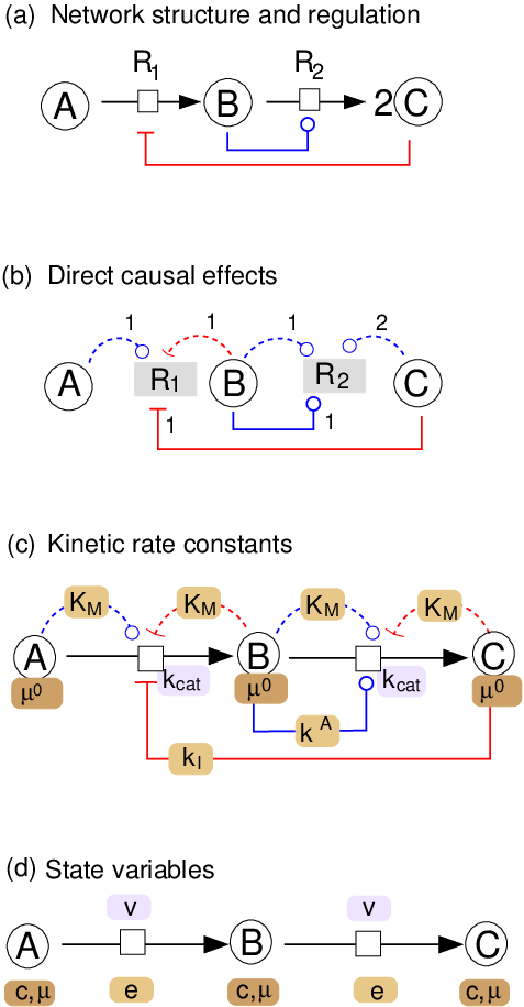

Modular rate laws [42] are generic reversible rate laws that capture various reaction stoichiometries, enzyme mechanisms, and types of regulation by effector molecules. Formulae for different rate laws and their elasticities can be found in [42] (supplementary material). As an example, let us consider a reaction without effectors. The common modular (CM) rate law is a reversible Michaelis-Menten kinetics, generalised for arbitrary stoichiometries. With two substrates A and B and one product C, it reads
| (9) |
with reactant constants , , and (in mM) and catalytic constants and (in s-1) for forward and backward direction. Modular rate laws can be adapted to different types of reactions and enzymes: if an enzyme is regulated by an effector molecule, this can be described, for example, by prefactors for activators X or for inhibitors Y. Moreover, with a Hill-like exponent the rate laws can capture sigmoidal kinetics. Other types of rate laws use the same parameters, but another denominator, for example, the saturable modular (SM) rate law
| (10) |
In the denominator, the substrate and product terms are simply multiplied. Modular rate laws assume an enzyme mechanism in which substrates and products bind rapidly, independently, and in random order. The reactant constants are dissociation constants of the elementary binding steps. Like the values in Michaelis-Menten kinetics, they denote reactant concentrations that would yield a half-maximal saturation (or -maximal saturation if ). The catalytic constants stem from the slow conversion step between substrate and product molecules. In all modular rate laws, the kinetic constants are required to satisfy Haldane relationships. One way to ensure this is to predefine the equilibrium constants, to treat the velocity constants as free parameters, and to compute the catalytic constants by using Eq. (17).
The kinetics and steady states of metabolic systems are constrained by thermodynamic, which defines relationships between metabolite concentrations , reaction rates , equilibrium constants , and chemical potentials . The chemical potentials are defined as the derivatives of the system’s total Gibbs free energy by the metabolite mole numbers . For ideal mixtures (metabolites at low concentrations in an aqueous solution, no mixture effects, activity coefficients of 1), the chemical potential of metabolite is given by the formula
| (11) |
with Boltzmann gas constant , absolute temperature , and chemical potential of metabolite at standard concentration22 2 For kinetic models, it is convenient to use a standard concentration of 1 mM, equal to the measurement unit for concentrations. In thermodynamic flux analysis, the common standard concentration is 1M. The conversion between the two conventions requires an adjustment of reaction Gibbs free energies, standard Gibbs free energies of formation, and equilibrium constants. . Here I omit the division by , assuming that all concentrations are given in units of the standard concentration. The ratio of product and substrate concentrations for a reaction is called mass-action ratio. In chemical equilibrium states, this ratio has always the same value, called equilibrium constant , which can be written as . The thermodynamic force , in a (possibly non-steady) metabolic state is defined as
| (12) |
It describes the Gibbs free energy dissipation (in kJ/mol) associated with a reaction event and can be computed from equilibrium constant and mass-action ratio (for reaction ):
| (13) |
In generalised Michaelis-Menten rate laws, the ratio of forward and backward rates of reaction is given by
| (14) |
The thermodynamic-kinetic formalism [77] defines the thermokinetic potential and splits it into , where is called capacity. For ideal mixtures (satisfying Eq. (11)), the thermokinetic potential is given by with a capacity , and related to via
| (15) |
In kinetic models, thermodynamic laws impose three sorts of constraints: a relation between flux directions and thermodynamic forces, Wegscheider conditions for equilibrium constants, and Haldane relationships between equilibrium constants and kinetic parameters. They arise as follows. (i) To carry a non-zero flux, chemical reactions must show a positive production of entropy per volume and time, (with the reaction affinity ). As a consequence, a (non-zero) reaction rate and the corresponding thermodynamic force must point in the same direction. (ii) The vector of logarithmic equilibrium constants ca be written as , with a vector of metabolite concentrations in an equilibrium state. For any such vector , the Wegscheider conditions have to be satisfied [78, 79] , where is a null space matrix satisfying . Similar Wegscheider conditions hold for all vectors of the form , including logarithmic mass-action ratios and thermodynamic forces . (iii) The fact that reaction rates vanish at chemical equilibrium implies a Haldane relationship between equilibrium constant and kinetic constants [18, 77]. For all modular rate laws, the Haldane relationship reads
| (16) |
To construct parameter sets that satisfy this relation, we define the turnover constants as the geometric means of forward and backward catalytic constants. By rewriting Eq. (16), we can now express the forward and backward catalytic constants as
| (17) |
These values satisfy the Haldane relationship by construction.
B.2 Reaction elasticities and thermodynamics
The derivatives between kinetic laws and enzyme concentrations , metabolite concentrations , or other function arguments are called reaction elasticities (see Figure 1 (a)). Given a rate law , the unscaled reaction elasticities are defined by derivatives
| (18) |
while the corresponding scaled elasticities are defined by logarithmic derivatives
| (19) |
Elasticities for other arguments of the rate law function (e.g. the enzyme level ) are defined accordingly. Scaled elasticities are dimensionless and can be seen as effective reaction orders: for mass-action kinetics, they are given by the substrate molecularities; for an enzyme that is fully saturated with the metabolite in question, they vanish. Scaled and unscaled elasticities can be interconverted by
| (20) |
and
| (21) |
Analogous conversion formulae hold for all types of sensitivities, including elasticities with respect to other parameters, control coefficients, and response coefficients [80, 16].
Elasticities depend on the rate laws, but also on thermodynamics. In reversible rate laws, the net reaction rate is the difference of forward and backward rates, whose ratio is determined by the thermodynamic force . The thermodynamic force, in turn, depends on reactant concentrations and equilibrium constant as (see Figure 1 (b)). If the thermodynamic force is large, the forward flux dominates and the net rate becomes sensitive to substrate fluctuations, but less sensitive to product fluctuations; therefore, the substrate elasticity increases and the product elasticity decreases. Near chemical equilibrium, where thermodynamic forces come close to zero, the scaled elasticities go to infinity.
The scaled elasticities of the SM rate law Eq. (10) contain the thermodynamic term as well as four terms that correspond to substrates, products, activators, and inhibitors:
| (22) |
For near-equilibrium reactions (small ) and for strongly driven reactions (), the first three terms can be approximated by
| (23) |
The last two terms in these formulae represent exactly the formula used in SKM [24], while the first term employs a thermodynamic correction. The scaled elasticities of the common modular rate law are a bit more complicated:
| (24) |
where (see [42]). Formulae for second-order elasticities, unscaled elasticities, parameter elasticities, and other types of modular rate laws can be found in [42].
For the factorized rate laws, and assuming a positive flux for simplicity, we obtain
| (25) |
where
| (26) |
STM relies on the fact that, given consistent fluxes and thermodynamic forces, any choice of the saturation values yields a consistent kinetic model and that any consistent model can be constructed in this way. This can be proven as follows. Consider a kinetic model with modular rate laws and a thermodynamically consistent flux distribution . For simplicity, enzyme levels are subsumed in the catalytic constants . As shown in [42], a consistent set of parameters, realising , can be obtained by the following procedure:
- 1.
Choose standard chemical potentials (free choice) and determine the equilibrium constants.
- 2.
Determine concentrations such that the signs of thermodynamic forces agree with the flux directions. If the metabolite concentrations are bounded, this may not always be possible, even if the flux distribution is loopless.
- 3.
Choose Michaelis constants and activation and inhibition constants and (free choice). Of course, given the previously chosen metabolite concentrations, this is equivalent to choosing the saturation constants (free choice in the range between 0 and 1) and computing the values from them.
- 4.
Set all velocity constants to preliminary values . Compute the catalytic constants from the Haldane relationships (16). Use the rate laws to compute the reaction rates . By construction (due to thermodynamically feasible metabolite levels and thermodynamically consistent rate laws), these rates have the same signs as the predefined fluxes. To match reaction rates and fluxes exactly, we just need to adjust the velocity constants, setting .
- 5.
If our flux distribution contains inactive reactions, we can decide, for each of them, whether we assume a vanishing thermodynamic force, a vanishing velocity constant, or a vanishing enzyme level. In the first case, we need to apply the strict energetic feasibility criterion for this reaction (i.e. require that the thermodynamic force vanishes); in the other cases, there is no feasibility criterion for the reaction, and the value or enzyme level is set to zero.
If this procedure yields correct models, this also holds for all models constructed by STM. In STM, we first determine consistent fluxes and thermodynamic forces that can be realised by a choice of standard chemical potentials and concentrations . Thus, when choosing the saturation constants, any choice is equivalent to a choice of , , and in the algorithm above. Thus, the quantities chosen until this point correspond exactly to the results of step 3. Thus, steps 4 and 5 will yield a unique, consistent set of parameters. Therefore, models obtained by STM satisfy all relevant constraints.
A main problem with SKM is that elasticities are sampled independently, which means that the resulting kinetic models may violate important constraints. If the forward and backward one-way rates of reactions were independent, and nont constrained by thermodynamics, an independent sampling would be justified: the elasticities could be directly translated into kinetic constants, and each sampled elasticity matrix would define a specific kinetic model. However, in models with reversible rate laws, independently sampled elasticities lead to inconsistent results. For example, consider a reaction A B with reversible mass-action kinetics : the scaled reaction elasticities read (for substrate A) and (for product B), so their difference is fixed. If we sample these elasticities independently, this relationship is violated and our sampled values cannot be realised by reversible mass-action rate laws. Similar constraints hold for all thermodynamically consistent reversible rate laws.
There can also be inconsistencies between the elasticities of different reactions. Here is a simple example: the reaction A B is catalysed by two isoenzymes with reversible mass-action kinetics:
| (27) |
The symbols and denote the concentrations of A and B, and and denote the rate constants. In each reaction, forward and backward kinetic constant must have the same ratio given by the equilibrium constant:
| (28) |
Therefore, the scaled elasticity matrix can be written as
| (29) |
with . All four elasticities are determined by the same parameter , so sampling them independently leads to a contradiction.
For a given modular rate law, the scaled elasticities can be computed from stoichiometric coefficients, thermodynamic forces, and saturation values. The fact that the same model details (e.g. the thermodynamic force of a reaction) have an influence on different reaction elasticities leads to dependencies between these elasticities: if these factors are varied, the resulting elasticities will be statistically dependent. Here is an example. When a thermodynamic force becomes larger, the substrate elasticities tend to increase and the product elasticities tend to decrease. When comparing all elasticities in a network, or when comparing the different instances of an ensemble model, this relationship between thermodynamic force and elasticities leads to positive correlations among substrate elasticities, positive correlations among product elasticities, and negative correlations between substrate and product elasticities in each single reaction. On the contrary, the unscaled elasticities in a pathway tend to increase with the pathway flux, leading to positive correlations between them (when comparing model instances with different flux distributions). Just like first-order elasticities are dependent, also the second-order elasticities are dependent on them. This entails statistical dependencies, both between the different sampled instances of a model (e.g., assuming different values of the thermodynamic forces) and between the reactions in a single model. Second-order elasticities tend to be negatively correlated with the product . To see this, consider a simple mass-action or power-law rate law without regulation: the elasticities are directly given by the thermodynamic terms
In this formula, the distinction between substrates and product is not made based on the actual flux direction, but on their roles in the reaction formula; the flux direction enters the formulae via , which may be larger or smaller than 1, depending on the sign of the thermodynamic force and thus on the flux direction. The second-order elasticities read
| (37) |
where, in the present case (non-regulated mass-action rate law), the prefactor reads
Due to this negative prefactor, we can expect a negative statistical correlation between the second-order elasticity and the product of first-order elasticities. In particular, close to equilibrium (where and therefore ), we obtain and thus the general formula , which is symmetric between substrates and products. For completely forward-driven reactions (with and ), in contrast, we obtain because the factor is close to 0. Can we expect the saxme relationship also for other rate laws? For generic saturable rate laws, a splitting as in Eq. (37) is formally possible, but there is no simple formula for . Therefore, a tendency for negative correlations between and may remain, but the negative correlation will be weaker.
B.3 Metabolic control theory
A steady state is a metabolic state in which metabolite levels and fluxes are constant in time. Steady-state fluxes and concentrations depend on enzyme levels and external metabolite levels . These dependencies may be complicated and not explicitly known (see Figure 8 (c)). However, if steady-state concentrations and fluxes are given, their sensitivities to parameter changes can be computed from the elasticities. The sensitivity between an target variable – e.g. a stationary concentration or a flux – and model parameters is called response coefficient. If each reaction has one reaction-specific parameter , for example the enzyme level , then we can divide the response coefficients by the elasticities and obtain the control coefficients (Figure 1 (c)). Control coefficients describe how local perturbations of a reaction rate affect the network-wide steady state. They are defined in such a way that they depend on the perturbed reaction, but not on which parameter caused the perturbation. Thus, response coefficients refer to perturbed parameters and control coefficients to perturbed reactions. The effects of global parameters such as temperature, which affect many reactions, are described by response coefficients (for more details, see SI E.2 and [80, 19, 16]). Elasticities, response coefficients, and control coefficients can be defined in their unscaled form (denoted by a bar ) or in their scaled form (denoted by a hat ) (see SI B.2). If an enzyme catalyses a single reaction, the enzyme level appears as a prefactor in the rate law and its scaled response and control coefficients are identical. The summation and connectivity theorems [15], a central finding in Metabolic Control Theory (MCT), entail linear dependencies among the control coefficients along a stationary flux distribution or in the reactions surrounding a common metabolite. Quantities and formulae related to fluctuations in time (such as spectral response coefficients, spectral power density, and variability on different time scales) are described in the SI.
The synergy effect of an enzyme pair on a flux (or on some other steady-state variable) can be approximated by second-order response coefficients, called synergy coefficients. Assume that two enzymes are inhibited, thus decreasing their levels and to small values and , and that this leads to relative flux changes , for the single inhibitions and for the double inhibition. Based on these numbers, we define the synergy effect
| (42) |
A positive value of indicates a buffering synergy (), while a negative value indicates an aggravating synergy (). If , there is no synergy. In a second-order expansion around the unperturbed state, the synergistic effect can be written as (see SI E.4)
| (43) |
so the scaled synergy coefficients quantify synergisms between two enzymes. If perturbations and target variables are measured on non-logarithmic scale, the synergistic effects can be approximated by with the unscaled response coefficient .
B.4 Model construction by STM
A kinetic steady-state model is determined by its network structure, rate laws, state variables, and saturation values: these values define the elasticities and kinetic constants. For a consistent model, these variables have to satisfy a number of constraints (C1-C5), explained by the dependency schema.
- •
Wegscheider conditions (C1). Some biochemical quantities, for example Gibbs free energies of reactions, can be written as differences along reactions, or in vector form , where is the stoichiometric matrix including both internal and external metabolites. Such quantities must obey the Wegscheider condition , where is a null-space matrix satisfying . Wegscheider conditions must hold, for example, for equilibrium constants (), mass-action ratios (), and thermodynamic forces ().
- •
Haldane relationships (C2). In a chemical equilibrium state, all metabolic fluxes must vanish. If we consider a single reaction in equilibrium, set its rate to zero (), and solve for the equilibrium constant, we obtain a equation between equilibrium constant and kinetic constants, the so-called Haldane relationship [81]. For example, for a reversible mass-action law the Haldane relationship reads . For the modular rate laws, it reads (see [42]).
- •
Equilibrium constant and chemical standard potentials (C3). In chemical equilibrium, the Gibbs free energies of reaction must vanish. With the formula for chemical potentials (i.e. assuming an activity coefficient and a standard concentration equal to 1), this leads to the formulae and .
- •
Signs of fluxes and thermodynamic forces (C4). According to the second law of thermodynamics, all chemical reactions must dissipate Gibbs free energy. This implies that rates and thermodynamic forces have the same signs ( and ), in agreement with the relationship . A stricter version of this constraint, excluding near-equilibrium reactions, is given below.
- •
Steady-state fluxes (C5). For applying MCT, the metabolic reference state must be a steady state, i.e. a state in which the metabolic fluxes satisfy the stationarity condition . In addition, we may impose bounds on the reaction rates and bounds on the production or consumption of external metabolites. Such bounds can be used to predefine reaction directions or to keep fluxes close to measured values.
- •
Stability (C6). For applying MCT to a metabolic reference state, this state must be asymptotically stable, i.e. its Jacobian matrix must not have eigenvalues with positive real parts. This constraint depends on all model details, and we cannot guarantee it be the dependency schema. Following [24], stable states can be obtained by generating a model ensemble and omitting all model instances with unstable states.
- •
Amounts or concentrations. In compartmentalised models, we need to distinguish between metabolites amounts and metabolites concentrations, which are related by compartment volumes. Generally, mass balances concern amounts while rate laws depend on concentrations. In STM, fortunately, amounts as such do not play a role. While concentrations appear as model variables, amounts are modelled only implicitly (e.g. if stationarity is imposed on fluxes).
If an algorithm for kinetic steady-state modelling violates these constraints, it leads to inconsistent models or metabolic states.

In a model with predefined kinetic constants, enzyme levels, and external metabolite concentrations, steady-state fluxes and concentrations can be determined numerically (Figure 9 (a)). However, to construct models with physiolocally plausible states, it may be safer to start from reasonable metabolic fluxes and to construct metabolite levels and kinetic rate laws around them in such a way that they yield the predefined fluxes (Figure 9 (b)). Model construction based on STM combines ideas from thermodynamic flux analysis [82, 12, 14] (in the metabolic state phase), SKM [24] and thermodynamically consistent model parametrisation [45, 77] (in the kinetics phase). Like in SKM, steady-state concentrations and fluxes can be predefined. To satisfy Wegscheider conditions, Haldane relationships, and the sign constraint between reaction rates and thermodynamic forces, steady state and kinetic constants are chosen sequentially. The network structure, our starting point, is defined by stoichiometric matrix, regulation matrix, and the list of external metabolites. In the algorithm, free variables (steady-state variables and saturation values) are determined step by step based on known values, constraints, or probability distributions: they can be chosen manually, by optimisation, by fitting them to data, or by random sampling. Dependent variables (e.g. kinetic constants) are computed from variables chosen previously, as prescribed by the dependency schema in Figure 2. Finally, models can be checked for a stable steady state (if such a state is required for the further analysis, e.g. Metabolic Control Analysis).
The scaled elasticities in STM resemble the saturation values as in SKM, but depend on saturation values and thermodynamic forces. Each sampled elasticity matrix corresponds to one instance of the model ensemble, that is, a particular kinetic model with consistent kinetic constants. In a variant of the algorithm, we do not sample the saturation values directly (, , ), but compute them from sampled dissociation constants (, and ). In both cases, the catalytic constants are computed from two constraints: the ratio is determined by the Haldane relationships while their geometric mean , treated as a model parameter , depends on their absolute scaling. To choose this scaling, we may either predefine the enzyme levels and scale the catalytic constants such that the reaction rate matches the predefined flux; or we predefine the values and solve for the enzyme levels.
Once the rate laws have been reconstructed, some of them may be replaced by laws obtained from enzyme assays to make the model more realistic [55]. To ensure a consistent model, the fluxes, concentrations, and equilibrium constants in these reactions must be equal between the reconstructed model and teh new rate laws to be inserted. There are different ways to guarantee this: either reaction rates and equilibrium constant, taken from the rate law, imposed as constraints when sampling the elasticities, or kinetic constants and enzyme level in the rate law are adjusted to the network model33 3 If an irreversible rate law is given, the equilibrium constant can be ignored in the network model.
Appendix C Model ensembles
C.1 Sampling the model variables
Our models represent samples from an ideal, infinitely large model ensemble defined by three types of information: (i) restrictions on model structure and steady state, set by the modeller (e.g. the choice of a fixed flux distribution); (ii) the independency between free variables, and dependencies of other variables on them, as encoded in the dependency schema (Figure 2); (iii) the random distributions from which the free variables are sampled. Together, these choices define the distributions and statistical dependencies of all model variables. Any kinetic model satisfying the constraints can be obtained by the algorithm.
In the metabolic state phase, a flux distribution may be chosen by flux minimisation. Metabolite concentrations, Gibbs free energies of formation, and thermodynamic forces may be determined by parameter balancing [52], using upper and lower bounds for concentrations and thermodynamic forces, known values (for concentrations) and predicted values (for Gibbs free energies of formation) as data, and flux directions as inequality constraints. Upper and lower bounds, signs, predefined values, and distributions used for sampling reflect model assumptions and available data; by choosing them, we can adjust the model to specific metabolic states and to kinetic or metabolic data. Fluxes and thermodynamic forces may be sampled uniformly, under linear constraints and with predefined sign patterns. Metabolite levels, enzyme levels, and dissociation constants can be sampled from log-normal or gamma distributions, and saturation values can be sampled, e.g., from uniform or beta distributions. In all phases of model construction, instead of sampling the variables freely, experimental data can be inserted, or distributions centred around data values can be used. To use experimental data in a more solid way, the entire model construction procedure can also be integrated into a Bayesian framework, in which a posterior for the model parameters is determined from data and priors.
To systematically study the impact of thermodynamic forces on model dynamics, one may vary the thermodynamic forces at a fixed metabolic flux distribution. Varying the thermodynamic forces (e.g. doubling all their values) requires a variation of metabolite levels, but these metabolite variations are not uniquely defined. For a simple procedure, we start from a metabolic state with concentration vector and force vector (which must agree with the flux directions). To realise a different force vector (with the same signs as ), we choose the new concentration vector
| (44) |
The idea is to apply a minimal overall change in metabolite concentrations (on logarithmic scale, and in the sense of an Euclidan distance). In this procedure, we may impose upper and lower bounds on . However, depending on the bounds there may be no solution.
C.2 Do model variants differ in their behaviour? Some useful statistical tests
Among the dynamic features of a metabolic model, which of them result from network structure and which depend mostly on quantitative factors like kinetic constants? To pose this question more generally, we may consider two model variants that differ in some aspect (e.g. network structure or flux distribution), while other aspects (e.g. rate constants) can be varied for each of the variants; then we ask whether a (qualitative or quantitative) model output differs significantly between the variants. To prove or disprove such differences, we describe each model variant by a model ensemble, sample instances from both ensembles, compute their target variables, and compare them for significant differences. This allows us, for example, to compare two variants of a kinetic model (with different network structures, synergies, steady-state fluxes, or expression patterns) and to check whether these differences lead to typical differences in their synergy patterns, irrespective of a variation of kinetic parameters. The test described below have been implemented in matlab (see github.com/liebermeister/stm).
If we ask about a qualitative model property (e.g. is the steady state stable or unstable?), each model ensemble can be characterised by the fraction of “positive” model instances. Given a set of sampled model instances (with count numbers and for “positive” and “negative” model instances), the true fraction can be estimated by Bayesian estimation. If were the true fraction, the number of positive model instances (out of model instances sampled) would be binomially distributed with mean and maximal value . Knowing this, we can estimate the value of from the given number by using Bayesian estimation. Assuming a flat prior, the posterior of is a beta distribution where and . The mean value of this distribution, can be used as an estimator for . The corresponding variance reads .
Given a matrix of enzyme synergies (where small-magnitude values have been removed by thresholding), we count the positive and negative synergies (numbers and ) between two groups of enzymes, e.g. between enzymes involved in two metabolic pathways. As a null hypothesis, we assume that synergies can be positive or negative with equal probabilities. Under this null hypothesis, and assuming that only very few synergies remain after thresholding, and would be independently binomially distributed with the same unknown mean value . Given , the difference would have a mean value of 0 and a standard deviation of . Thus, the ratio between an observed difference and this standard deviation can be used as a score for sign bias. Since the value of is unknown, we approximate it by and obtain the empirical sign bias score .
Finally, we consider quantitative target variables and their differences between model variants as seen in model ensembles. As an example, we consider predicted enzyme synergies. The general idea is as follows. To see whether a synergy (between two enzymes and ) differs significantly between two model variants, we compute the synergies for many instances of the two model variants, take the mean value for each variant, and compare the two values using a p-value (obtained from a permutation test) as a criterion for significant differences. Since we run many such tests in parallel (namely, for many different enzyme pairs), we expect a certain amount of false positives. To account for multiple testing, we choose a false discovery rate and select significant enzyme pairs based on their p-values [83]. This is how the procedure works in detail:
- 1.
Sample synergy values We sample model instances for each of the two model variants. For each model instance, we compute the synergies of all enzyme pairs. Altogether, we obtain a collection of synergy values , indexed by for enzyme pairs, for the two model variants, and for the sampled model instances of each variant. If the network contains enzymes, there are enzyme pairs, i.e. possible synergies to be computed. The synergy data are now tested for significant differences.
- 2.
Quantify large (positive or negative) synergies by p-values For each enzyme pair , we first test whether this pair shows a significantly large (or small) synergy value caused by the model structure, i.e. if it does, the synergy values will stand out from the general distribution of synergy values, even if we average over many random choices of the kinetic parameters. We apply the following statistical test: for each enzyme pair , we test whether the mean value (from the two model variants and all Monte Carlo samples) is significantly larger (or smaller) than other mean synergy values. We use a permutation test: the actual mean value for our enzyme pair is compared to mean values obtained from batches of resampled values. In each permutation run , we resample of the values with replacement and compute their mean value . Let denote the number of resampled mean values larger than . Whether is significantly large is indicated by a p-value , estimated by
(45) (for a justification, see the above treatment of binary variables). Small values indicate that is larger than expected by chance (i.e. significantly large), large values indicate that it is smaller than expected by chance (i.e. significantly small).
- 3.
Quantify differences in synergies (between model variants) by p-values Next, for each enzyme pair , we ask whether the synergy values differ significantly between the two model variants. In the test, we consider the mean values and of the two model variants, averaged over all kinetic parameter samples, and check whether they differ significantly. Again, we use a permutation test. This time, we compute the mean difference . In each run of the the permutation test, we randomly permute the values for the pair under study, divide them into two batches of size , and compute the mean difference between the two batches. A p-value, stating whether is large, for is computed as above, by counting how many of the permutation samples lead to larger values.
- 4.
Select significant synergies or differences based on p-values Given the previously computed p-values, we determine which of their mean values and of their mean differences are significantly high (or low). Since we test this for many gene pairs, we need to account for multiple testing: we fix a false discovery rate of 5% and choose the confidence level for the individual tests. With this choice, of the apparently significant values (for each of the four tests, high or low mean synergy and difference in synergy) are expected to be false positives.
C.3 Extensions of STM
The algorithm for model construction can be extended in many ways:
- •
Cell compartments In kinetic models with compartments, the compartment sizes appear in the balance equations and may follow differential equations themselves. In our model construction, compartments are not modelled explicitly, but a compartment structure can be added to the reconstructed kinetic model. This, however, changes control properties such as Jacobian, response, and control matrices.
- •
Dilution by cell growth. In models with dilution (due to growth rate ), intracellular metabolites will be effectively “consumed” by a dilution flux . This changes the stationarity condition and directly couples fluxes to metabolite levels. Given a steady state, the elasticities can be computed as normally, but the Jacobian, response, and control coefficients will be affected. The elasticities for the dilution reactions are directly given by dilution rate and metabolite levels.
- •
Thermodynamically infeasible fluxes. Eq. (1), the main formula in elasticity sampling, requires that flux directions follow the thermodynamic forces, that is, fluxes must lead from higher to lower chemical potentials. In practice, even valid flux distributions may violate this assumption, for example, if cofactors or protons are omitted in the model. To apply STM regardless, we may choose to ignore thermodynamics and treat some reactions as irreversible – that is, we ignore the thermodynamic term in the substrate elasticity and set the product elasticity to zero. Alternatively, we may adjust the thermodynamic forces to the given flux directions: whenever differs from the flux direction, we add a virtual substrate and choose its chemical potential such that the thermodynamic force has the correct sign. The virtual substrate changes the equilibrium constants and thermodynamic forces, but can otherwise be ignored in the kinetic rate law.
- •
Avoiding divergencies close to chemical equilibrium. In reactions close to chemical equilibrium, with a thermodynamic force , the one-way rates and scaled elasticities become very large. This does not only cause numerical problems, but also implies a very fast or very abundant enzyme, to sustain a finite flux at an enzyme efficiency close to 0. To avoid this in our models, we set a constraint on the forward and backward rates in each reaction. With a threshold , for example, forward fluxes can be at most 100 times as large as the net flux. This translates into a constraint for thermodynamic forces in the metabolic state phase: the flux sign constraint () is replaced by the stricter constraint44 4 The constraint can be derived as follows (assuming without loss of generality): the ratio between forward and net reaction rate is given by . Close to equilibrium, we can approximate and obtain . . It will prevent extreme values in the thermodynamic elasticity term . The unscaled elasticities, in contrast, do not diverge in chemical equilibrium and can be computed from non-divergent formulae [42].
- •
Enzyme reactions composed of elementary steps. If we think of enzyme mechanisms as composed of elementary mass-action steps, we also represent them in this way in a model, replacing each reaction by a more fine-grained description. In the resulting model, there is a much larger number of (elementary) reactions. Since all rate laws are mass-action kinetics, the elasticities are directly given by reversibility terms and completely determined by thermodynamic forces. It sounds surprising: by knowing the fluxes and thermodynamic forces, we completely know the enzme kinetics! But we should not forget that we are now talking about the thermodynamic forces of elementary steps and that the equilibrium constants of these steps corresponds to values (of saturable modular rate laws) in the more coarse-grained model.
- •
Prior distributions for saturation values. Saturation values can be set to fixed values (e.g. for enzymes believed to be in the linear range, for enzymes in half-saturation, or for enzymes in full saturation), or they can be sampled independently from the range . If is drawn from a uniform distribution (as suggested by the principle of minimal information [84]) and the metabolite levels are fixed, the resulting dissociation constant is randomly distributed with probability density (see SI E.1). If a saturation value is approximately known, we can use a beta distribution instead, with density with a mean value given by the known value. This yields a distribution for the dissociation constant. Saturation values can also be sampled from dependent distributions: this may be necessary if enzymes bind to different reactants, for example NAD+ und NADH, with unknown but similar binding affinities, leading to correlations between their saturation values in physiological states.
- •
Multiple steady states. Under different choices of external metabolite levels and enzyme levels, a kinetic model will show different steady states. Each of these states is characterised by different metabolite levels, fluxes, saturation values, and elasticities. For constructing a model with multiple states directly, STM to be modified: we need to ensure that the saturation values and elasticities in different states correspond to the same set of kinetic constants. However, this is simple. In the metabolic state phase, we sample a set of equilibrium constants and different sets of state variables for the multiple steady states; in the kinetics phase, we sample a single set of kinetic constants, which then determine the saturation values, elasticities, and enzyme levels for each steady state. Again, enzyme levels are determined last from the other variables; the only way to adjust them – e.g. to proteome data – is by surrounding the algorithm into another layer of parameter fitting or posterior sampling.
- •
Adaptation of enzyme levels. In our metabolic models, enzyme levels appear as parameters. In reality, they are controlled by transcriptional regulation, an important mechanism for shaping metabolic behaviour. To include transcriptional regulation into our metabolic models, the model must be extended to describe the production of enzymes. Alternatively, we may treat enzyme levels as choice variables and attempt to derive plausible enzyme adaptation profiles from optimality considerations [20]. To improve metabolic efficiency, enzymes should be expressed in the right proportions, to be adapted continuously to the current metabolic tasks. For instance, a rising demand for a certain metabolite may lead to an induction of a biosynthesis pathway for this metabolite. If such feedback systems are in place, changes in enzyme levels will affect the metabolic state, and induce secondary adaptations of other enzymes, and so on. For predicting the effects of, e.g. gene knock-downs, we need to consider the global interplay of such adaptations. Given a kinetic model with a metabolic objective function and an enzyme cost function, optimal enzyme adaptations to external changes or single-enzyme knock-downs can be predicted with the help of synergy coefficients [20]. Again, the predicted enzyme adaptations reflect network structure and elasticities.
- •
Analysis of sampled target variables. A model ensemble can be seen as a statistical model with independent (“free”) and dependent (“determined”) variables. The dependencies are described by a schema like the one from Figure 2. Each binary property (e.g. the sign of a control coefficient) has a certain probability in the ensemble. In practice, we can only estimate this probability from a limited number of model instances. If out of sampled models show the property , the probability of , called , can be estimated as follows: assuming that has a uniform prior, its posterior mean and variance read and . For each target variable (e.g. a control coefficient), we obtain a number of sampled values. Their distribution can be characterised by mean value, variance, probabilities of signs, and correlations with other model variables.
- •
Significant differences between model variants. By choosing network structure, fluxes, thermodynamic forces, and enzyme saturation step by step, we can realise a nested sampling that leads to a hierarchy of model variants. In this hierarchy, each model variant is represented by a model ensemble with a specific distribution of target variables. To make them comparable, model variants should at least have the same metabolite and reaction lists, but they can differ in their network structures and in the values assigned to any of the free variables. Using statistical tests, we can determine significant differences between the distributions of model targets, if necessary with corrections for multiple testing (see section C.2 for details). By comparing the distributions of model variables between subensembles, we can study how structural model features affect the target variables: for example, whether certain regulation arrows can enhance the stability of steady states. More generally, we can systematically study the effects of network structure, regulation, thermodynamic forces, enzyme saturation, and different rate laws on our model outputs.
- •
Choosing the distributions of target variables. To see how specific values or ranges of target variables can be obtained, we can build a model ensemble and then filter it for models that show these values or ranges. Again, we obtain a subensemble of models with different distributions and correlations of the model variables. Even free variables that were chosen independently can become dependent by the subselection. Alternatively, we can set the distribution our target variables during model construction by applying a Bayesian posterior sampling. In this approach the “free” variables are not sampled freely but by a Metropolis Monte Carlo procedure: as prior distributions we can choose the same probability distributions as usually; for the likelihood function, we compare the resulting target variables to the prescribed distribution, for example, a distribution defined by experimental data.
C.4 Example model: glycolysis in human hepatocytes
In the original publication [59], thermodynamically feasible fluxes were determined by flux minimisation with various different flux objectives. I first focused on aerobic rephosphorylation of ATP on glucose. Optimising this objective leads to a sparse flux distribution that uses only a small part of the network, containing glycolysis and TCA cycle. With this flux distribution, I first determined a standard model in which all saturation values were set to values of 1/2, assuming half-saturated enzymes. In the resulting state, the steady ATP rate (our model output) is strongly controlled by glucose import; all control coefficients are positive, i.e. a small increase of any enzyme would always increase the metabolic target (ATP level). Although the flux distribution was chosen to support ATP rephosphorylation, this is not a trivial finding: first, flux analysis can capture the ATP rephosphorylation rate, but not the ATP level as a target function; second, it describes which fluxes – and in which proportions – are optimal to realise a certain metabolic objective, but it does not capture the marginal effects of enzyme levels, i.e. how the objective would change upon small enzyme changes. By sampling the saturation values, we obtain a model ensemble, and the statistical distribution and correlations of these control coefficients can be studied.

Appendix D Metabolic synergies and fluctuations
(a) Flux analysis (b) Metabolic control theory
| FBA 0.1 | MoMA 0.1 | CM Half-saturation | SM Half-saturation |
|---|---|---|---|
 |
 |
 |
 |
 |
 |
 |
 |
| FBA 0.9 | MoMA 0.9 | CM Ensemble mean | SM Ensemble mean |
 |
 |
 |
 |
 |
 |
 |
 |
D.1 Synergies between static perturbations
Synergy effects between enzymes can be important in medical applications, e.g. to model drug interactions or patient-specific side effects, to plan combination therapies, and to avoid the emergence of bacterial resistance [85]. Epistasis, an important concept in genetics, denotes the synergistic effects of gene knockouts on cell viability. Epistasis can shape genetic variability in populations and the evolvability of genetic features. Moreover, as shown by FBA simulations and experiments, epistatic interactions can indicate functional associations between proteins, for example the cooperation or alternative usage of enzymes in metabolic pathways [56]. Importantly, while synergies are described here for enzyme perturbations, they can also be computed and used for any other parameter perturbations, including synergistic effects between concentrations in the growth medium.
Epistatis describes synergy effects of gene deletions on Darwinian fitness. In buffering epistasis between two genes (double-deletion phenotype is less severe than expected), the loss of one gene lowers the selection pressure on the other one: in evolution, such genes will tend to co-occur in genomes, a phenomenon called phylogenetic correlation [86]. In th eopposite case, called aggravating epistatis, the double-deletion phenotype is more severe than expected: the loss of one gene increases the selection pressure on the other one, leading to phylogenetic anti-correlation. In [56], epistatic synergies in the yeast S. cerevisiae were computed by FBA. The maximal biomass production rate was used as a quantitative output function and enzyme deletions were simulated by setting the corresponding reaction rates to zero. The predicted epistasis pattern showed a modular structure [56].
Segrè et al. introduced a synergy score for double enzyme deletions [56], in which a special weighting makes buffering synergies better detectable. Let denote an target variable (e.g. maximal biomass production rate computed by FBA) observed in the wildtype network, and let , , and denote the values in mutatnt networks in which enzyme a, enzyme b, or both have been deleted. After a scaling by the wildtype value, the target values read , , and . Since deletions can decrease, but cannot increase the target in FBA, the values must satisfy , , and . The effect of a double deletion is compared to the effects and of single deletions, yielding an epistasis score. To obtain a clear distinction between neutral (), aggravating (), and buffering (), gene pairs, Segrè et al introduced a heuristic epistasis measure with the following definition:
In the formula for buffering epistasis, we assume without loss of generality. In summary, neutral and aggravating synergies are defined “normally”, but buffering synergies are given special weights: if one of the single-deletion effects is mild, then is close to 1 and the buffering synergy is increased by this definition. If both single deletions are already severe, then the buffering synergy gets a lower weight.
FBA, MoMA, and MCT all predict enzyme synergies, but based on different assumptions and input data. For double inhibitions, all three methods predict, not surprisingly, that cooperating enzymes (i.e. enzymes in one linear pathway) tend to show buffering synergies, while alternative enzymes (e.g. enzymes in alternative pathways) show aggravating synergies. However, the reasons for these predictions, their details, and other predictions differ between the methods. An example is shown in Figure 5. As expected, a double inhibition that block both alternative routes has an aggravating effect, while enzymes within the same linear pathway show buffering synergies. MCT explains this by control coefficients: in the first case (across alternative pathways), inhibition of one branch increases the flux control of the other branch, while in the second case (within one linear pathway), the first enzyme inhibition decreases the flux control of all other enzymes (see Fig. (11)).
D.2 Metabolic fluctuations
To model a metabolic pathway under dynamic external perturbations, we may model these perturbations as a random process. The perturbations themselves, and the resulting metabolite fluctuations are described by spectral power density matrices. These matrices resemble the static covariance matrices, but are frequency-dependent. If the noise amplitudes are small, we can use a linearised model and compute the spectral densities of concentration fluctuations from the spectral response coefficients [22]
| (50) |
and denote the spectral power densities of metabolites and of perturbation parameters at circular frequency , the symbol indicates the adjoint matrix, and the unscaled first-order spectral response matrices and can be computed from the elasticities [21, 22]. For fluctuations of reaction rates, there is a similar formula.
An important example of random fluctuations is chemical noise. On a microscopic scale, chemical reactions do not run continuously as assumed in kinetic models, but as discrete random events, converting individual molecules. The resulting random dynamics can be described by a Langevin equation, i.e. a kinetic model with additive noise and separate forward and backward rates [68]. The fluctuations spread in the network, leading to fluctuations of molecule numbers in the macroscopic steady state. In the Langevin equation, the noise term scales with the square root of the mean reaction rate (in units of reaction events per second). Therefore, the smaller the particle numbers, the bigger the relative noise. If the average rates become very small, the approximation breaks down and a more detailed model with discrete reaction events must be used. The fluctuations can be described by Eq. (50), setting (where marks once-way fluxes) and , because the chemical fluctuations originate from white noise (see [22]). In practice, the spectral power density of the original noise in reaction is given by
| (51) |
where the approximation holds close to equilibrium (small thermodynamic force ). Mediated by the metabolic dynamics, these input fluctuations lead to fluctuations of metabolite levels and fluxes (for an example, see Fig 13). Fast fluctuations are strongly damped: the noise spectrum of the metabolite levels decreases at high frequencies, and the system acts as a low-pass filter. Since each reaction rate is also directly affected by its own noise, fluxes also fluctate at high frequencies. If a stable metabolic state is close to a Hopf bifurcation, it will show a tendency towards oscillations. This becomes visible apparent in the way it transmits random fluctuations, and in its noise spectrum: noise will be amplified around a resonance frequency close to the oscillation frequency after the Hopf bifurcation. All this can be seen from the eigenvalue spectrum of the Jacobian matrix [22].
For low or high frequencies, the noise amplitudes can be understood through simple approximations. The spectral power density matrix for metabolite fluctuations has the form with a diagonal matrix . The noise variances for individual metabolites, at specific frequencies, are given by diagonal values
| (52) |
The spectral response matrix itself is given by , with matrices and and the Jacobian matrix . For large frequencies ( much larger than any eigenvalue of the Jacobian), the term dominates and the entire expression (52) becomes proportional to . High-frequency noise is dominated by direct effects of chemical noise on the adjacent reactant levels, i.e. fast, non-stationary fluctuations around the stationary fluxes. For low frequencies, in contrast, the spectral power density approaches the variability expected for static variability, and the correlations reflect slow, stationary variations of the stationary fluxes.
The amplitude of random fluctuations at specific frequencies are described by the spectral power density. However, in reality we are usually not interested at the noise level at a precise frequency, but at noise affecting processes on a certain time scale, where much faster noise averages out and much slower noise can be seen as quasi-static. To measure the relevant noise on a time scale of interest, we consider a noisy curve from our model, e.g. of a metabolite level, compute a sliding average with a Gaussian kernel (of width , e.g. one second), and study how much this average varies (across the statistical ensemble at one point in time, or along time in one realisation of the process). Alternatively, we can also consider a sliding average with. By changing the width of the kernel, we obtain the variance of our metabolite curve on different time scales. This measure of concentration fluctuations at different time scales can be computed from the spectral power densities using a Fourier transformation (see section E.3).
(a)

(b)
| Fast noise (1 s-1) | Frequency dependency | Slow noise (0.001 s-1) |
|---|---|---|
 |
 
|
 |
D.3 Role of thermodynamics and enzyme saturation in metabolic control and fluctuations
Thermodynamic forces and saturation values have effects on metabolic control and fluctuations. Figure 13 shows these effects for a simple model, a pathway of five uni-uni reactions without regulation. In the standard model version, all thermodynamic forces are set to RT and all saturation values are set to 1/2. To assess the effects of parameter changes, the parameters in the third reaction were systematically varied, setting the force to values of 0.1 RT, RT, and 10 RT, while keeping the metabolite concentrations close to their original values (see section C.1). Similarly, the (substrate and product) saturation values were set to values of 0.1, 0.5, and 0.9. The figure shows static control coefficients and spectral power densities of chemical noise (for metabolite levels and fluxes). There are some clear patterns: if the third reaction is close to equilibrium (0.1 RT), it has little control on concentrations and fluxes, and also little influence on the control exerted by other reactions. In contrast, if the reaction is strongly driven, it exerts a larger control, while the control exerted by downstream enzymes, and all control on downstream metabolites decreases. If the reaction is close to equilibrium, the substrate saturation does not play a role; as the reaction is driven strongly, the substrate saturation additionally increases the control exerted by the reaction. Thus, for a high flux control, reaction must be strongly driven and the enzyme must be saturated with substrate.
(a) Variation of thermodynamic forces
| Chemical potentials | Thermodynamic forces | ||
|---|---|---|---|
| 0.1 RT |  |
 | |
| 1 RT |  |
 | |
| 10 RT |  |
 |
(b) Control coefficients
Concentrations
Fluxes
0.1
0.5
0.9
0.1 RT


 1 RT
1 RT


 10 RT
10 RT


 0.1
0.5
0.9
0.1
0.5
0.9


Appendix E Mathematical derivations
E.1 Probability densities for saturation values and dissociation constants
The fraction of enzyme molecules (of one sort of enzyme) bound by a certain metabolite depends on the metabolite concentration and on the dissociation constant (indices omitted for simplicity). It can be described by saturation values or . The saturation values are directly related to and . If is uniformly distributed in the interval , the conditional probability densities read
| (53) | |||||
| (54) |
Similar formulae hold for the sampling of . According to this formula, follows a logistic distribution with location parameter 0 and scale parameter 1. Mean, median and mode of are given by 0, and the variance is given by
Proof: The probability density of is . For fixed parameter , we obtain and thus
| (55) |
The normalisation constant has a value of 1 because
| (56) |
For fixed concentration , we compute and obtain
| (57) |
again with normalisation constant because
| (58) |
E.2 Metabolic control and response coefficients
Control and response coefficients describe the effects of small parameter changes on state variables (metabolite concentrations and reaction rates ) in a first- or second-order approximation [15, 16]. The unscaled response and control coefficients can be computed from the unscaled elasticities and the stoichiometric matrix [22]. In systems without conservation relations, the first-order unscaled control matrices read
| (59) | |||||
| (60) |
In models with linear conservation relations, the Jacobian is rank-deficient and not invertible, but we can still compute the control coefficients [80]: we select a set of independent internal metabolites (such that the reduced matrix has full row rank, and the same rank as ). Then the stoichiometric matrix can be split into a matrix product , and Eq. (59) is replaced by
| (61) |
The response matrices with respect to system parameters read
| (62) |
Scaled control and response matrices, e.g. , are defined similar to the scaled elasticities. Since the enzyme concentrations appear as prefactors in the rate laws, it turns out that scaled response coefficients and scaled control coefficients are identical. With other perturbation parameters (e.g. external metabolite concentrations), this will not be the case.
For general perturbation parameters and (i.e. not necessarily enzyme levels), we can write the unscaled synergy tensors [19] as
| (63) |
with a tensor defined as
| (64) |
Enzyme levels are parameters with specific properties: there is only one enzyme per reaction, and enzyme levels appear as prefactors in the rate law. Thus, for two enzyme levels and we obtain the unscaled response coefficients (see Eq. (85))
| (65) |
The scaled synergy coefficients between a steady-state variable and enzyme levels and read (see Eq. (86))
| (66) | |||||
The synergy coefficients describe second-order effects of an enzyme (indices ) or synergies of enzyme pairs (indices ). For enzyme pairs, the Kronecker vanishes and we can set (see Eq. 59). By rewriting the second-order elasticities as in Eq. 37 and rearranging Eq. (66), we obtain
| (67) |
For mass-action rate laws close to equilibrium and without regulation, the term is approximately -1.
E.3 Spectral power density and temporal variability due to chemical noise
To describe metabolic fluctuations caused by chemical noise, we use the chemical Langevin equation
| (68) |
for particle numbers ,The reaction propensities denote the probabilities per time (in s-1) for events of reaction in forward (+) or backward (-) direction, and and are vectors of standard Gaussian white noise55 5 The white noise appears in the formula as the derivative of a standard Wiener process. It has the covariance function (in s-1) and a spectral power density (unitless). Note the prefactor convention used for Fourier transforms: and . (in units of s-1/2). In a cell volume , molecule numbers and propensities are related to concentrations and reaction rates as
| (69) |
with Avogadro’s constant mol-1. using these variables, we can rewrite the chemical Langevin equation as
| (70) |
For deviations from a stationary state, and setting , we can approximate it by
| (71) |
with the unscaled elasticity matrices
| (72) |
in units of s-1 and mM s-1/2, respectively. Eq. (71) has the form of a standard linear model with perturbation parameters in a vector . For this model, we can compute the frequency-response matrices (see [22])
| (73) |
in units of mM s1/2 and mol s-1/2, respectively. The concentration fluctuations have the spectral power density matrices
| (74) |
(in mM2 s). An analogous formula holds for flux fluctuations (in mol2 s-1). To study fluctuations on a specific time scale (in units of seconds), we consider the fluctuating concentration curve and smoothen it by convolving it with a (normalised) Gaussian function of width . The resulting function has the spectral power density
| (75) |
The function in brackets is the Fourier transform of our Gaussian function. The covariance function of the smoothed curve is given by the reverse Fourier transform of the spectral power density
| (76) |
The variance (the covariance function for time shift ) is therefore given by
| (77) |
An analogous formula holds for the covariance of flux fluctuations.
E.4 Synergy effects
Here we derive the Eq. (43 for synergy effects. The effect of a double enzyme perturbation on an target variable can be seen as the sum of three terms: the single-inhibition effects plus a synergy effect :
| (78) |
The synergy effect , defined as the difference , can be approximately determined from the metabolic response coefficients. Given a vector of enzyme changes, a second-order Taylor expansion yields
| (79) |
Therefore, if two enzyme concentrations and are decreased by and , the target changes by
| (80) |
The single perturbations yield
| (81) |
With the second-order approximation Eqs (79) and (80), the synergy effect is given by the unscaled synergy coefficient multiplied by the perturbations:
| (82) |
If all quantities (enzyme levels and target variable) are measured on logarithmic scale, it is natural to consider the splitting
| (83) |
It corresponds to a “null hypothesis” of multiplicative effects, contains the scaled synergy , and in the corresponding formulae the scaled response coefficients are used.
E.5 Response and synergy coefficients
here we derive Eq. (66 for scaled synergy coefficients. The unscaled synergy cofficients (second-order response coefficients) between general parameters and and state variables (stationary concentrations and fluxes) read (as in Eq. (63) and using Einstein’s sum convention):
| (84) |
If the perturbation parameters are enzyme levels and , we can write the elasticities as , , , and set . By inserting this into Eq. (84), we obtain
| (85) | |||||
which is equivalent to the formula given in [19]. The scaled synergy coefficients read, in analogy to Eq. (20),
| (86) | |||||
They can be written – again with sum symbols – as
| (87) |
The previous formulae holds for targets that are stationary concentrations or fluxes . How can we generalise them to other target variables , which are functions of these state variables ? Let the unscaled derivatives be called and . We shall first first compute the unscaled, and then the scaled response coefficients of . The unscaled response coefficients read (with sum convention)
| (88) |
For the next step, we introduce the scaled derivatives and . With their help, we write the unscaled derivatives as
| (89) |
The unscaled synergy coefficients for our target read
| (90) | |||||
Let us now consider the scaled response coefficients. The first-order scaled response coefficients read
| (91) |
The scaled synergy coefficients read (compare Eq. 88)
| (92) | |||||
For functions that are multiplicative in fluxes and concentrations (i.e. linear if all quantities are given on logarithmic scale), the first term vanishes.