Reconstruction and uniqueness of moving obstacles

Let $\Omega_{1}(t)$ be a reflecting convex moving obstacle with a smooth boundary in a domain $\Omega_{0}$ and $\overline{\Omega_{1}(t)}\subset\Omega_{0}\subseteq\mathbb{R}^{3}$. Consider an ultrasonic wave, or signal, described by the wave equation

where $c(x,y,z)>0$ is the variable speed of sound in $\Omega(t)=\Omega_{0}\backslash\overline{\Omega_{1}(t)}$. We consider as positive the speed of sound at each point of the domain which is not inside an obstacle and define

and

for $t>0$. When $\Omega_{1}(t)=\emptyset$ then $\Omega(t)=\Omega_{0}$ and therefore we consider that the speed of sound in $\Omega_{0}$ is positive and known when there is no obstacle present.

We model the signals as rays and look for solutions of the wave equation. These solutions of the wave equation [1] are called rays or ray solutions [2]. We model $\Omega_{0}$ to be an environment without caustics.

Let $f(x,y,z)=\frac{1}{c(x,y,z)}>0$ in $\Omega$. Suppose that for all t we are given all integrals $\int_{\gamma}f(l)dl=C_{\gamma}(t)$ where $\gamma$ are broken rays in $\Omega_{0}$ reflecting at $\partial{\Omega_{1}(t)}$. A broken ray is a ray reflecting at the obstacle and is defined as the union $\gamma=\gamma_{1}\bigcup\gamma_{2}$ of two rays $\gamma_{1}$ and $\gamma_{2}$ in $\Omega_{0}$ starting at the observation boundary and intersecting at the obstacle’s boundary. Then as we know $C_{\gamma}(t)$ correspond to signal travel times in a medium with speed of sound $c(x,y,z)$. The shape and trajectory reconstruction problem is to find $\partial{\Omega_{1}(t)}$ given the sets $C_{\gamma}(t)$ of travel times where $\gamma\in\Omega_{0}$, the initial and end positions and take off angles of the rays $\gamma$, and the speed of sound in the whole domain when there is no obstacle present.

In our model for the shape and trajectory reconstruction problem rays start at signal transmitters and end at signal receivers with known locations in the observation boundary $\partial{\Omega_{0}}$. In addition, we model the rays to have known initial conditions: the initial zenith and azimuth angles at the transmitter as well as the times when signals are sent are recorded and are known. Receivers can record the times when signals are received and these times are known as well. The combined information from transmitters and receivers provides the data or data points

for the shape and trajectory reconstruction problem where where $\phi_{k}$ and $\theta_{k}$ are the initial incident and azimuth angles of the ray with index k from its transmitter, $x_{kl}$, $y_{kl}$, $z_{kl}$ are the coordinates of the transmitter endpoint of the ray, and $x_{kr}$, $y_{kr}$, $z_{kr}$ are the coordinates of the receiver endpoint of the ray, $t_{k}$ is the travel time for the signal and $\xi_{k}$ is a frequency of the signal.

The ray paths of unbroken rays with known initial conditions are solutions of a system of equations used in the Shooting Method for two-point seismic ray tracing[3]:

Systems of equations that present an initial value formulation for the ray equations have origins in acoustics [4] and are used in algorithms for seismic ray tracing [5, 6, 7]. In other imaging fields, such as non-destructive testing and biomedical imaging, non-linear ultrasound is studied with a focus on frequency methods[8, 9]. This work provides a mathematical definition and solution of the shape and trajectory reconstruction problem and is focused on reconstruction and uniques of moving obstacles.

In the above system of equations (x(t), y(t), z(t)) is the ray position vector, $\phi(t)$ is the incident angle of the ray direction vector with the z axis and $\theta(t)$ is the azimuth angle that the projection of the ray direction vector makes with the positive x axis.

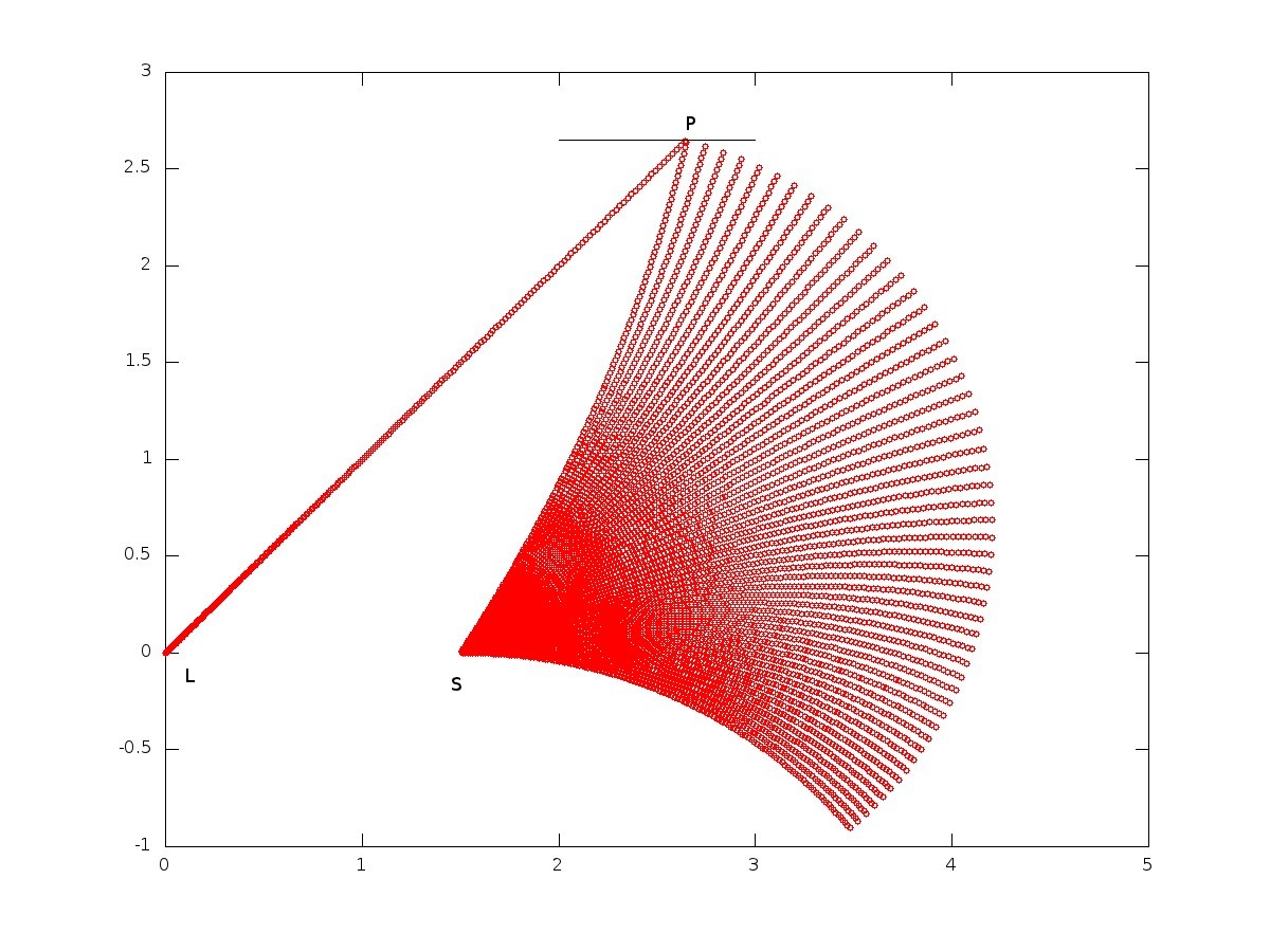
In order to reconstruct the obstacle, we consider the speed of sound $c(x,y,z)$ to be positive and known throughout $\Omega_{0}$ when there is no obstacle present and trace rays from transmitters and receivers as if there is no obstacle. When the sum of ray travel times at an intersection point of a transmitter and a receiver ray is equal to the travel time $t_{k}$ from the corresponding data point, we infer that the intersection point could be a reflection point from $\partial{\Omega_{1}}(t)$. The algorithm is described in the paper on shape and trajectory reconstruction of moving obstacles[10] and its operation is shown in Figure 1.

This work extends the above algorithm with a filtering phase which ensures that the reconstructed solution is unique and contains only points from $\partial{\Omega_{1}}(t)$. This work also extends the first phase of the reconstruction algorithm for computing all reflection points that meet the initial conditions with an adaptive computation of the time step for tracing transmitter and receiver branches of broken rays. We then analyse the conditions for existence and uniqueness of the solution.

The reconstruction algorithms work in two phases. The first phase finds all points in $\Omega_{0}$ that are intersection points of transmitter and receiver rays with initial conditions from the data and for which the sum of travel times of the traced rays from transmitter and receiver endpoints to the intersection point is equal to the travel time from the corresponding

data point. This section presents the first phase of the algorithm. The next section describes and analyses the second filtering phase.

The input to the following algorithm is the speed of sound $c(x)$ for the domain $\Omega_{0}$ when there is no obstacle present and a set of data points or ray coordinates corresponding to the initial conditions of broken rays and their travel times. The output is a set of points in $\mathbb{R}^{3}$ reconstructed from the input data.

The algorithm uses a Runge-Kutta method for the RK step and is flexible to work with other time-dependent numerical methods. When the algorithm is parallelized and caching and other optimization techniques are used then its computational complexity is $O(T)$ where T is the number of discretization points for the travel time of a broken ray. For input $\{B_{k}\}$ from one sampling time interval $T_{k}$, the algorithm reconstructs the shape of the obstacle during this sampling interval and the trajectory of the obstacle is reconstructed when the algorithm is run on the data points for each of the sampling intervals. Resolution of the reconstruction can be very high because the reconstruction method allows collection and processing of a large number of data points corresponding to different points from $\partial{\Omega_{1}(t)}$. Reconstruction with high resolution by the above algorithm of a neighborhood of points from a moving obstacle is shown in Figures 2, 3, 4, 5 and 6.

For a transmitter at $L$ and receiver at $S$ the travel time between L and S along a broken ray $\gamma$ with segments $\gamma_{1}$ and $\gamma_{2}$ and reflection point $P$ is

For a fixed $t$ and constant speed of sound c the above equation implies that the set of points P is an ellipsoid with focci $L$ and $S$. This can be seen by multiplying both sides of the equation by $c$ which leads to

which is the equation of an ellipsoid with focci $L$ and $S$.

Therefore, for constant speed of sound $c$ and a data point with transmitter $L$, receiver $S$, initial angles $\phi$ and $\theta$ and travel time t, a unique point P can be reconstructed because a ray from L with initial angles $\phi$ and $\theta$ travelling along a straight line, because of the constant speed of sound, will intersect the ellipsoid in exactly one point P.

For variable speed of sound $c(x,y,z)$ the set of points $P$ is a surface $K$ which is not necessarily convex. In this case a ray from L with given initial conditions and travelling along a curve could intersect the surface $K$ in more than one point. In other words there can be several rays from the receiver that intersect the transmitter ray at different points such that for each intersection point the sum of travel times from transmitter and receiver to the intersection point is equal to the total travel time.

In order to find the unique reflection point for the measurement ray, the above algorithm is extended by adding a second filtering phase after the first phase of the algorithm. The first phase finds all solution points for which the sum of travel times from transmitter and receiver to the solution point is equal to the travel time from the data point. The filtering phase finds the unique reflection point by reconstructing the shape via several pairs of transmitters and receivers and selecting those points which have been recontructed by a sufficiently large threshold number $q$, $q\geq 3$, of (transmitter, receiver) pairs. This implies that the data must contain at least q data points with different transmitter receiver pairs for each reconstructed point. Therefore, the observation boundary must contain a sufficient number of transmitters and receivers that are located so that each point in $\partial{\Omega_{1}}(t)$ is seen from at least q transmitter receiver pairs. The algorithm with the combined first and second phases is as follows.

The proof of the correctness of the filtering phase and uniquess conditions on the input data are as follows.

Sketch of proof: For each data point $B_{k}$ the first phase of the above reconstruction algorithm finds one or more solution points $P_{1}$,…,$P_{m}$. Only one of these solution points is the unique reflection point P for $B_{k}$’s measurement ray. The remaining solution points for $B_{k}$ will be referred to as intangible solution points. The conditions of the theorem guarantee that for P there are at least q data points with different transmitter receiver pairs and this implies that P will be counted at least q times by the algorithm. The probability $p_{k}$ that any one of the intangible solution points is also an intangible solution point for another data point and its measurement ray is less than 1 and depends on the discretization of the numerical solution. Therefore, the probability that any one of the intangible solution points is counted at least q times by the second phase of the algorithm and each of these times it is an intangible solution point for the corresponding data point is less than or equal to ${(p_{k})}^{q-1}$. For sufficiently large q this probability tends to 0, therefore, with probability one, solution points that are not unique reflection points for at least one measurement ray will be filtered out by the algorithm. Therefore, the conditions of the theorem guarantee that for each $B_{k}$ a unique reflection point P with count greater than or equal to q exists because each point from the obstacle’s boundary is measured from at least q different transmitter receiver pairs.

Consider a circular reflecting obstacle with Lambertian reflectance in the plane xy moving away from the origin along the line $x=y$ in a medium with variable speed of sound $c(x,y)=x+y+1$. We place a transmitter and a receiver at the origin. In this case, the domain $\Omega_{0}$ is a circle of sufficiently large radius that contains the origin. Table 1 shows the computation by the algorithm from section 2 of the trajectory of a point on the obstacle on the line $x=y$ corresponding to data with different travel times from different sampling periods.

We check whether the computation of the above table by the algorithm from 2 is correct as follows. The time for the ray to reach to obstacle can be computed by the formula

Therefore,

By symmetry, for this particular example, this time t is half of the total travel time T. Then for a travel time $T=2$, or $t=1$, we compute $X=Y=1.55$. This result matches the corresponding result for xp and yp from Table 1 obtained by numerical integration. For $T=1.75$ the numerical computation gives $xp\neq yp$ while by the above formula $X=Y$. In this case, the relative error between the values computed by the algorithm and the value computed by the formula is less than 1 percent.

In order to reconstruct more points from $\partial{\Omega_{1}(t)}$ we can vary the transmission angles. Table 2 shows that by varying $\theta$, the initial angle at which we transmit rays from transmitter, we can reconstruct points on the boundary of the circular obstacle. In contrast, in Table 1 both $\phi$ and $\theta$ are constant. In order to reconstruct the boundary with higher resolution we can change the initial angles $\theta$ and $\phi$ in smaller steps. Figure 5 and Figure 6 show how changing the initial angle $\theta$ at the transmitter in smaller steps leads to higher resolution of the reconstruction.

The speed of the obstacle $v(T)$ must be sufficiently slow compared to the speed of the signals $c(x,y,z)$ during every sampling period so that for the signal travel times T from one sampling period, i.e. the times in column T where the sampling period $\Pi$ is the same, for time period $\delta$, where

the obstacle does not move by a noticeable amount. $\Pi$ denotes the index or unique id of a sampling time period and $d(\Pi)$ the duration of this time period. Therefore, the duration $d(\Pi)$ of the sampling time period $\Pi$, during which rays are sent from the transmitter in order to reconstruct the boundary of the obstacle when it is approximately stationary, must be less than or equal to $\delta$ or

Combining the images of the obstacle from successive sampling intervals reconstructs the shape and trajectory of the moving obstacle.

The reconstruction tests show that for high resolution and performance it is essential that the method is run adaptively. In addition to changing the time step, the reconstruction accuracy can be tuned by changing the number of tested angles at the receiver.

The above algorithm adapts the angle resolution and via the algorithm from section 2 it adapts the time step.

In floating point arithmetic

where $t_{LP}$ is the time for the transmitter segment, $t_{PS}$ is the time for the receiver segment and t the total travel time for the broken ray. The check from the algorithm

implies that there are many points that are sufficiently close to a solution. The error is determined by the constants $\epsilon_{1}$ and $\epsilon_{2}$ and it is necessary to choose sufficiently small constants for reconstruction with high accuracy and resolution. Therefore, reconstruction of a point is unique within a ball of sufficiently small diameter which depends on the constants $\epsilon_{1}$ and $\epsilon_{2}$.

The error of the solution is also determined by the sum of the two errors from the numerical integrations for the rays from transmitter and receiver. In addition, the error of the solution is determined by discretization errors. The initial angles at the receiver from the numerical solution belong to a finite set of initial angles that are tried. The differences between the initial angles $\theta_{c},\phi_{c}$ from the numerical solution and real angles $\theta_{i},\phi_{i}$ for the ray at the receiver are

and

These differences are guaranteed to be sufficiently small when the initial angles space is tested in sufficiently small equal steps.

One performance optimization of the algorithm for shape and trajectory reconstruction of moving obstacles is the use of a data structure or a database for looking up points on the receiver rays for a given discretization of the initial angles space. Consider a cover of $\Omega_{0}$ by a finite number of cubes. Let M be a cube, $\Omega_{0}\subset M$, centered at the origin and with sides parallel to the xy, yz and xz planes. Let $l_{m}$ be the length of one side of $M$ and divide $M$ into cubes with side length $b=\frac{l_{m}}{N_{v}}$ where $N_{v}$ is a natural number that determines the resolution of the mesh. Assign each of the cubes with side b from the resulting mesh a unique natural number from 1 to ${N_{v}}^{3}$. All precomputed points on receiver rays are stored in a database table RT with the following schema:

The region column corresponds to the number of the cube from the mesh to which point $(x,y,z)$ belongs. The region or cube number of a point can be defined by the function

The optimized first phase of the algorithm with a fixed time step and lookup of cached receiver rays is as follows.

References

• [1] Eskin G. Lectures on Linear Partial Differential Equations, Graduate Studies in Mathematics, vol. 123. American Mathematical Society: Providence, Rhode Island, 2011.
• [2] VMBabicˇ\check{c}, Buldyrev V. Short-Wavelength Diffraction Theory. Springer Verlag: Berlin Heidelberg, 1991.
• [3] Julian B, Gubbins D. Three-dimensional seismic ray tracing. J. Geophys. 1977; 43:95–1113.
• [4] Eliseevnin V. Analysis of waves propagating in an inhomogeneous medium. Soviet Physics 1965; Acoustics(10):242–245.
• [5] Sambridge M, Kennet B. Boundary value ray tracing in a heterogeneous medium: a simple and versatile algorithm. Geophys. J. Int. 1990; 101:157–168.
• [6] Červený V. Seismic Ray Theory. Cambridge University Press: Cambridge, 2001.
• [7] Bleinstein N, Cohen J, Stockwell J. Mathematics of Multidimensional Seismic Imaging Migration and Inversion. Springer Verlag: New York, 2001.
• [8] Arnold W, Hirsekorn S ( (eds.)). Acoustical Imaging, vol. 27. Springer Netherlands.
• [9] Pasovic M, Danilouchkine M, van Neer P, Cachard C, Van Der Steen AFW, Basset O, De Jong N. Second harmonic inversion for ultrasound contrast harmonic imaging. Physics in Medicine and Biology 2011; 56(11).
• [10] Lozev K. Algorithms for shape and trajectory reconstruction of obstacles in domains with variable speed of sound. J. Physics Conf. Ser. 2013; 410(012171):1–4.