Turing Instability in Reaction-Diffusion Systems with a Single Diffuser: Characterization Based on Root Locus

©2013 IEEE. Personal use of this material is permitted. Permission from IEEE must be obtained for all other uses, in any current or future media, including reprinting/republishing this material for advertising or promotional purposes, creating new collective works, for resale or redistribution to servers or lists, or reuse of any copyrighted component of this work in other works.

Hiroki Miyazako Yutaka Hori Shinji Hara ^†^†thanks: H. Miyazako, Y. Hori and S. Hara are with the Department of Information Physics and Computing, The University of Tokyo, Tokyo 113-8656, Japan. {Hiroki_Miyazako, Yutaka_Hori, Shinji_Hara}@ipc.i.u-tokyo.ac.jp

Abstract

Cooperative behaviors arising from bacterial cell-to-cell communication can be modeled by reaction-diffusion equations having only a single diffusible component. This paper presents the following three contributions for the systematic analysis of Turing instability in such reaction-diffusion systems. (i) We first introduce a unified framework to formulate the reaction-diffusion system as an interconnected multi-agent dynamical system. (ii) Then, we mathematically classify biologically plausible and implausible Turing instabilities and characterize them by the root locus of each agent’s dynamics, or the local reaction dynamics. (iii) Using this characterization, we derive analytic conditions for biologically plausible Turing instability, which provide useful guidance for the design and the analysis of biological networks. These results are demonstrated on an extended Gray-Scott model with a single diffuser.

1 Introduction

In biological compartments, spatial diffusion of molecules can lead to an ordered spatial pattern of chemical concentrations (see [9, 10] for examples). The dynamical model of such diffusion-driven pattern formation, or Turing pattern formation, was first introduced by Turing [14] as a reaction-diffusion system. Then, intensive efforts during the past half-century have revealed essential mechanisms of diffusion-driven instability, or Turing instability, such as the activator-inhibitor theory [5, 8, 4].

In recent synthetic biology, researchers have attempted to design gene regulatory networks that result in spatially patterned gene expression over a population of bacterial cells [2, 1]. One of the ideas to realize such a biological circuit is to utilize a cell-to-cell communication mechanism mediated by a diffusible molecule called an autoinducer [11]. We can then expect that the diffusion of the autoinducer drives a certain spatial mode and generates spatial patterns of gene expression. In contrast to the classical ones, the reaction-diffusion model for such system has a distinctive feature that there is only one diffusible molecule, or the autoinducer, in the system. Thus, a novel theoretical framework is desirable to systematically study reaction-diffusion systems having only one diffusible component.

In particular, there still remains an important fundamental question that whether Turing patterns can be generated in reaction-diffusion systems with a single diffuser. This question was partly tackled in the recent theoretical study [7], where a gene regulatory network showing spatial patterns was proposed. Our study, however, has verified that the patterns emerging from the examples in [7] result in extremely fine spatial patterns dominated by infinitely large spatial frequency, which is biologically implausible. Hence, it is desirable to theoretically characterize biologically plausible Turing instability and to develop a systematic way to explore the conditions for such instability.

This paper presents the following three contributions on reaction-diffusion systems with a single diffuser.

(i)

We propose a unified framework to systematically formulate the reaction-diffusion system as an interconnected multi-agent dynamical system.
(ii)

We then characterize biologically plausible and implausible Turing instabilities by the root locus of the local reaction dynamics.
(iii)

Using this characterization, we derive analytic conditions for biologically plausible Turing instability.

In particular, our analysis proves that it is possible to generate biologically plausible patterns only with a single diffusible molecule. These results provide useful guidance for the design of synthetic biological circuits.

The organization of this paper is as follows. In the next section, we introduce the reaction-diffusion system considered in this paper and formulate it as a multi-agent dynamical system. In Section III, we mathematically define biologically plausible and implausible Turing instabilities. Then, in Section IV, these instabilities are characterized by the root locus. In Section V, we derive analytic conditions for the biologically plausible Turing instability. Then, Section VI is devoted to the demonstration of our result on an extended Gray-Scott model [15]. Finally, Section VII concludes this paper.

The following notations are used throughout this paper. $\mathbb{C}_{+}:=\{s\in\mathbb{C}~|~\mathrm{Re}[s]>0\}$ and $\mathbb{C}_{0+}:=\{s\in\mathbb{C}~|~\mathrm{Re}[s]\geq 0\}$ . $\mathbb{R}_{\geq 0}:=\{c\in\mathbb{R}~|~c\geq 0\}$ . $\mathbb{N}:=\{1,2,3,\cdots\}$ .

2 Control Theoretic Formulation of Reaction Diffusion Systems

In this section, we first introduce reaction-diffusion systems with a single diffuser and show that the systems can be viewed as multi-agent dynamical systems.

2.1 Reaction-Diffusion systems with a single diffuser

We consider a set of chemical reactions consisting of $n$ molecular species, $\mathcal{M}_{1},\mathcal{M}_{2},\cdots,\mathcal{M}_{n}$ , in one dimensional space $\Omega:=[0,L]$ . Let $x_{i}(\xi,t)$ denote the concentration of $\mathcal{M}_{i}~(i=1,2,\cdots,n)$ at position $\xi\in\Omega$ and at time $t$ , and define ${\bm{x}}(\xi,t):=[x_{1}(\xi,t),x_{2}(\xi,t),\cdots,x_{n}(\xi,t)]^{T}$ ¹¹ 1 In what follows, we may denote ${\bm{x}}(\xi,t)$ by ${\bm{x}}$ to avoid notational clutter. . In this paper, we consider the case where only $\mathcal{M}_{n}$ can diffuse in the spatial domain. The dynamics of the reactions and diffusion is then given by

\displaystyle\frac{\partial{\bm{x}}}{\partial t}=f({\bm{x}})+D{\bm{\nabla}}^{2}{\bm{x}},

(1)

where the nonlinearity $f(\cdot)$ is a Lipschitz continuous function representing the dynamics of local reactions, and $D:=\mathrm{diag}(0,\cdots,0,\mu)\in\mathbb{R}_{\geq 0}^{n\times n}$ is the matrix with a diffusion coefficient $\mu$ . It should be noted that only the $(n,n)$ -th entry is non-zero, since only $\mathcal{M}_{n}$ can diffuse. Throughout this paper, we assume the Neumann boundary condition as follows.

\displaystyle\frac{\partial{\bm{x}}}{\partial\xi}(0,t)=0,~~\frac{\partial{\bm{x}}}{\partial\xi}(L,t)=0.

(2)

We here introduce a linearized model of (1) to analyze Turing patterns based on local stability analysis in the following sections. Let $\bar{{\bm{x}}}\in\mathbb{R}_{\geq 0}^{n}$ denote a spatially homogeneous equilibrium of (1). The linearized system around $\bar{{\bm{x}}}$ is then obtained as

\displaystyle\frac{\partial\tilde{\bm{x}}}{\partial t}=A\tilde{\bm{x}}+D{\bm{\nabla}}^{2}\tilde{{\bm{x}}},

(3)

where $A\in\mathbb{R}^{n\times n}$ is the Jacobian of $f(\cdot)$ evaluated at $\bar{{\bm{x}}}$ , and $\tilde{\bm{x}}$ is defined by $\tilde{{\bm{x}}}:={\bm{x}}-\bar{{\bm{x}}}$ .

2.2 Formulation as a multi-agent dynamical system

Refer to caption — Figure 1: Block diagram of the system (2.2).

The linearized model (3) can be equivalently written as

\displaystyle\begin{array}[]{cc}\displaystyle\frac{\partial{\tilde{{\bm{x}}}}}{\partial t}=A\tilde{{\bm{x}}}+{\bm{e}}_{n}u\\ y={\bm{e}}_{n}^{T}\tilde{{\bm{x}}},\end{array}

where $u=\mu\nabla^{2}y$ and ${\bm{e}}_{n}:=[0,\cdots,0,1]^{T}\in\mathbb{R}^{n}$ . The equations (2.2) imply that for each fixed position $\xi$ , the dynamics of local reactions, which we denote by $h(s)$ , can be modeled as a SISO linear time-invariant system with the input $u(\xi,t)$ and the output $y(\xi,t)$ . Specifically, $h(s)$ can be written as

\displaystyle h(s):={\bm{e}}_{n}^{T}(sI_{n}-A)^{-1}{\bm{e}}_{n}~(=:n(s)/d(s)),

(6)

where we define $n(s)$ and $d(s)$ as the numerator and the denominator of $h(s)$ , respectively. The reaction-diffusion system (2.2) can then be interpreted as the feedback system illustrated in Fig. 1, where $\mathcal{I}$ is an identity operator, and $\nabla^{2}=\partial^{2}/\partial\xi^{2}.$ Note that this system can be viewed as a multi-agent dynamical system, where the homogeneous dynamical agents $h(s)$ are coupled with the nearest neighbor agents by the Laplace operator, and the stability analysis of such class of systems was studied in [13, 6].

The infinitely large-scale multi-agent system can be decomposed into small subsystems by diagonalizing the Laplace operator $\nabla^{2}$ as $\mathcal{F}\nabla^{2}\mathcal{F}^{-1}=\mathrm{diag}[h(s),h(s),\cdots]$ with the Fourier transform operator $\mathcal{F}$ . The eigenvalues $\lambda_{k}$ and the associated eigenfunctions $\phi_{k}(\xi)$ of $-\mu\nabla^{2}$ are specifically obtained as

\displaystyle\lambda_{k}\!:=\!\mu\left(\frac{k\pi}{L}\right)^{2},~\phi_{k}(\xi)\!:=\!\cos\left(\frac{k\pi\xi}{L}\right)

(7)

for $k=0,1,2,\cdots$ . Consequently, the closed-loop system in Fig. 1 can be decomposed into the subsystems $\Sigma_{k}~(k=0,1,2,\cdots)$ depicted in Fig. 2.

It should be noticed that the dynamics of each subsystem $\Sigma_{k}$ represents that of each spatial mode $\phi_{k}(\xi)$ . In fact, it follows that

\displaystyle\tilde{{\bm{x}}}(\xi,t)=\sum_{k=0}^{\infty}\hat{{\bm{x}}}_{k}(t)\cos\left(\frac{k\pi\xi}{L}\right),

(8)

where $\hat{{\bm{x}}}_{k}$ is the state of the subsystem $\Sigma_{k}$ as depicted in Fig. 2. In particular, the spatial pattern formation is expected when the growth rate of a non-zero spatial mode $\phi_{k}(\xi)~(k=1,2,\cdots)$ is positive. Therefore, the analysis of pattern formation in reaction-diffusion systems reduces to the stability analysis of the small subsystems $\Sigma_{k}$ .

Let the characteristic polynomial of the closed-loop system composed of $h(s)$ and a gain $\lambda$ be denoted by

\displaystyle p(\lambda,s):=d(s)+\lambda n(s).

(9)

The characteristic polynomial of each subsystem $\Sigma_{k}$ is then written as $p_{k}(s):=p(\lambda_{k},s)$ . Thus, a subsystem $\Sigma_{k}$ is asymptotically stable, if and only if $p_{k}(s)$ is Hurwitz. Moreover, we can also see that the linear infinite dimensional system (3) is exponentially stable if and only if $p_{k}(s)$ is Hurwitz for all $k=0,1,2,\cdots$ ²² 2 We can prove this since the Laplace operator is a Riesz spectral operator, though the proof of the sufficiency requires careful treatment in general infinite dimensional linear systems (see Section 5 of [3] for details)..

3 Definitions of Biologically Plausible and Implausible Turing Instability

In this section, we first introduce the definition of Turing instability, by which the reaction-diffusion system exhibits spatial patterns. Then, the Turing instability is classified into two types from a viewpoint of biological plausibility.

Definition 1. The reaction-diffusion system with a single diffuser modeled by (1) is Turing unstable around an equilibrium $\bar{{\bm{x}}}$ , if

(i) $p_{0}(s)=d(s)\neq 0$ ; $\forall s\in\mathbb{C}_{0+}$ and
(ii) $p_{k}(s)=0$ ; $\exists s\in\mathbb{C}_{0+}$ and $\exists k\in\mathbb{N}\cup\{\infty\}$ .

That is, (i) all the poles of $\Sigma_{0}$ lie in the open left half-plane, i.e., $A$ is Hurwitz, and (ii) at least one pole of $\Sigma_{k}$ lies in the close right half-plane for some $k=1,2,\cdots$ .

We can see that at least one non-zero spatial mode has a positive growth rate around the equilibrium when the system (1) is Turing unstable. Thus, we expect that the reaction-diffusion system exhibits a spatial pattern after a small perturbation to the homogeneous equilibrium $\bar{\bm{x}}$ . It should be noticed that the stability of $\Sigma_{0}$ implies that the dynamics of local reactions $h(s)$ is stable, i.e., $A$ is Hurwitz, thus Turing instability is exclusively driven by the diffusion of the molecule $\mathcal{M}_{n}$ .

When there are multiple unstable subsystems $\Sigma_{k}$ , the spatial profile of the pattern depends on the growth rate of the subsystems’ outputs. More specifically, the spatial mode corresponding to the most unstable subsystem tends to be dominant as $t\rightarrow\infty$ . Thus, the rightmost pole of the closed-loop system is of particular interest in our study.

Definition 2. A pole $\sigma$ of $\Sigma_{k}$ is called a dominant closed-loop pole, if (i) $\mathrm{Re}[\sigma]\geq 0$ and (ii) $\sigma$ has the largest real part among all the poles of $\Sigma_{k}~(k=0,1,2\cdots)$ . More precisely, the set of all dominant poles is defined by

	$\displaystyle\Pi:=\{$	$\displaystyle s_{0}\in\mathbb{C}_{0+}~\|~p_{k}(s_{0})=0;\exists k\in\mathbb{N}\cup\{\infty\},\mathrm{and}$
		$\displaystyle p_{k}(s\!+\!\mathrm{Re}[s_{0}])\neq 0;k\in\mathbb{N}\!\cup\!\{\infty\}~\mathrm{and}~\forall s\!\in\!\mathbb{C}_{+}\}.$

When the dominant pole is given by a subsystem $\Sigma_{k}$ , the output of $\Sigma_{k}$ has the largest growth rate , thus the $k$ -th spatial mode is expected to appear at steady state.

The following definition further classifies Turing instability into two types based on the location of the dominant pole. Note that the notation $\mathbb{N}$ does not include infinity.

Definition 3. The reaction-diffusion system with a single diffuser modeled by (1) is Type-I Turing unstable around an equilibrium $\bar{{\bm{x}}}$ , if the following (A) and (B-I) are satisfied. Similarly, it is Type-II Turing unstable if the following (A) and (B-II) are satisfied.

(A) The system is Turing unstable.
(B-I) $p_{k}(s_{0})=0$ ; $\exists k\in\mathbb{N}$ and $\exists s_{0}\in\Pi$ .
(B-II) $p_{k}(s_{0})\neq 0$ ; $\forall k\in\mathbb{N}$ and $\forall s_{0}\in\Pi$ .

In other words, the system is Type-I Turing unstable, if the dominant closed-loop pole is given by $\Sigma_{k}$ with some finite $k$ , and it is Type-II Turing unstable, if the dominant closed-loop pole is the pole of $\Sigma_{k}$ as $k\rightarrow\infty$ .

Figure 3 illustrates the two types of Turing instability and the corresponding spatio-temporal evolutions of the diffuser. In what follows, the spatial patterns associated with Type-I and Type-II Turing instabilities are referred to as Type-I and Type-II Turing patterns, respectively.

We see from Fig. 3 that the dominant spatial mode is expected to be infinite for Type-II Turing patterns, while it is finite for Type-I Turing patterns. The spatial patterns with the infinitely large spatial mode are, however, questionable from a viewpoint of biological plausibility. Thus, we shall explore the conditions for Type-I Turing instability, which excludes the biologically implausible patterns in Section V.

Remark 1. Definitions 1,2 and 3 can also be used when there are multiple diffusers in the system. For such cases, the characteristic polynomial $p_{k}(s)$ can be obtained by $p_{k}(s)=|sI-A+\lambda_{k}\hat{D}|$ , where $\hat{D}:=\mathrm{diag}(\mu_{1},\mu_{2},\cdots,\mu_{n})$ . Nevertheless, the classification of Type-I and Type-II Turing instabilities was not actively studied in the classical works of reaction-diffusion systems [12, 4] where the systems are composed of $n=2$ molecules and both can diffuse in the spatial domain. This is because such a system is always Type-I Turing unstable, when it is Turing unstable. On the other hand, Type-II Turing instability can happen when the number of diffusers is restricted. In [7], it was shown that a reaction-diffusion system with one diffuser can exhibit Turing instability, but the classification of the instability was not discussed. In fact, the examples presented in [7] are classified into Type-II Turing instability. Hence, there still remains an important question that whether Type-I Turing instability, which is physically plausible, is possible in reaction-diffusion systems with a single diffuser. $\hfill\Box$

4 Characterization of Turing Instabilities by Root Locus

In this section, we show that the two types of Turing instability introduced in the previous section can be characterized by the root locus of $h(s)$ , which is the local reaction dynamics. This characterization then leads to analytic conditions for Type-I Turing instability in the next section.

It should be first noticed that $\Sigma_{k}$ is a negative feedback system with the feedback gain $\lambda_{k}$ defined in (7), and the feedback gain $\lambda_{k}$ monotonically increases in terms of $k$ . This implies that the poles of the subsystems $\Sigma_{k}~(k=0,1,2,\cdots)$ lie on the root locus of the local reaction dynamics $h(s)$ . In other words, the poles of the subsystems $\Sigma_{k}~(k=0,1,2,\cdots)$ move from the poles toward the zeros of $h(s)$ as $k\rightarrow\infty$ . This allows us to characterize the two types of Turing instabilities using the root locus of $h(s)$ as seen below.

In order to examine the root locus in detail, we partition the matrix $A\in\mathbb{R}^{n\times n}$ as

A=\left[\begin{array}[]{c:c}\tilde{A}\hfil\lx@intercol\vrule\lx@add@cssclass&{\bm{b}}\\ \hline\cr{\bm{c}}\hfil\lx@intercol\vrule\lx@add@cssclass&d\end{array}\right],

(10)

where $\tilde{A}\in\mathbb{R}^{(n-1)\times(n-1)},{\bm{b}}\in\mathbb{R}^{n-1},{\bm{c}}\in\mathbb{R}^{1\times(n-1)}$ and $d\in\mathbb{R}$ . The matrix $\tilde{A}$ represents the interactions between non-diffuser molecules, and $d$ is the production or degradation rate of the single diffusible molecule. The vectors ${\bm{b}}$ and ${\bm{c}}$ express the interactions between the non-diffusers and the diffuser. Then, the denominator $d(s)$ and the numerator $n(s)$ of $h(s)$ can be specifically calculated as follows.

Lemma 1. The local reaction dynamics $h(s)$ is written as

\displaystyle h(s)=\frac{n(s)}{d(s)}=\frac{|sI_{n-1}-\tilde{A}|}{|sI_{n}-A|}.

(11)

Proof. We first note that

\displaystyle h(s)=\frac{{\bm{e}_{n}}^{T}\mathrm{adj}(sI_{n}-A){\bm{e}_{n}}}{|sI_{n}-A|},

(12)

where $\mathrm{adj}(X)$ represents the adjugate matrix of $X$ . It follows from the definition of the adjugate matrix that the $(n,n)$ -th entry of $\mathrm{adj}(sI_{n}-A)$ is $|sI_{n-1}-\tilde{A}|$ . Thus, ${\bm{e}}_{n}^{T}\mathrm{adj}(sI_{n}-A){\bm{e}}_{n}=|sI_{n-1}-\tilde{A}|$ . $\hfill\Box$

Remark 2. Lemma 1 provides an important physical interpretation of the denominator and the numerator of $h(s)$ . Specifically, we can see that that the zeros of $h(s)$ are determined from the dynamics of the non-diffusers, $\mathcal{M}_{1},\mathcal{M}_{2},\cdots,\mathcal{M}_{n-1}$ , which is specified by $\tilde{A}$ . The poles are, on the other hand, determined from the overall local reaction dynamics including the diffuser $\mathcal{M}_{n}$ . This implies that the starting and the ending point of the root locus can be characterized by these two dynamics. $\hfill\Box$

The following lemma summarizes the relation between the stability of subsystems $\Sigma_{k}~(k=0,1,2,\cdots)$ and the root locus of $h(s)$ .

Lemma 2. The poles of $\Sigma_{k}~(i=1,2,\cdots)$ are given by the roots of

\displaystyle p(\lambda,s)=d(s)+\lambda n(s)=|sI_{n}-A|+\lambda|sI_{n-1}-\tilde{A}|=0

with $\lambda=\lambda_{k}$ . In particular, they are given by $\mathrm{spec}(A)$ for $k=0$ and move to $\mathrm{spec}(\tilde{A})$ as $k\rightarrow\infty$ .

We can see that that the difference between Type-I and Type-II Turing instabilities essentially boils down to the relation between the dominant closed-loop pole and the terminal point of the root locus (see Fig. 3). In particular, Lemma 2 implies that the terminal of the root locus is $\mathrm{spec}(\tilde{A})$ . In the next section, these properties allow us to analytically explore conditions for Type-I Turing instability.

We note that the poles of $\Sigma_{k}~(k=0,1,2,\cdots)$ are discrete, whereas the root locus of $h(s)$ is continuous in terms of the feedback gain $\lambda$ . Thus, careful treatment is necessary to rigorously study instability conditions based on the root locus. In practice, however, the length of the spatial domain $L$ is sufficiently large such that the discrete feedback gains $\lambda_{k}=\mu(k\pi/L)^{2}~(k=0,1,2,\cdots)$ are close to each other. Moreover, our interest here is not the instability induced by the size of the domain but the diffusion of a molecule. Hence, following the convention [12, 4], we hereafter analyze Turing instability under the next assumption.

Assumption 1. We assume $L$ is sufficiently large such that if $p(\lambda,s)=0$ for some $\lambda>0$ and some $s\in\mathbb{C}_{+}$ , then $p(\lambda_{k},s)=0$ for some $k\in\mathbb{N}\cup\{\infty\}$ and some $s\in\mathbb{C}_{+}$ .

5 Conditions for Type-I Turing Instability

In this section, we first provide a general necessary and sufficient condition for Type-I Turing instability in reaction-diffusion systems with one diffuser. Using this condition, we further explore Type-I Turing instability for systems composed of $n=2$ and $n=3$ molecules.

5.1 Necessary and sufficient condition

We can first derive the following necessary and sufficient condition for Type-I Turing instability from Lemma 2.

Lemma 3. Consider the reaction-diffusion system with a single diffuser modeled by (1). This system is Type-I Turing unstable around $\bar{{\bm{x}}}$ , if and only if (i), and (ii-a) or (ii-b) hold.

(i) $A$ is Hurwitz.

(ii-a) $\tilde{A}$ is Hurwitz, and

\displaystyle\mathrm{Re}[p(\lambda,j\omega)]=0,~~\mathrm{Im}[p(\lambda,j\omega)]=0

(13)

for some $\lambda>0$ and some $\omega\in\mathbb{R}$ .

(ii-b) $\tilde{A}$ is not Hurwitz, and

\displaystyle\mathrm{Re}[p(\lambda,\beta+j\omega)]=0,~~\mathrm{Im}[p(\lambda,\beta+j\omega)]=0

(14)

for some $\lambda>0$ and some $\omega\in\mathbb{R}$ , where $\beta:=\max_{\nu\in\mathrm{spec}(\tilde{A})}\mathrm{Re}[\nu]$

The conditions (ii-a) and (ii-b) guarantee that the rightmost zeros of the local reaction dynamics $h(s)$ are not identical with the dominant closed-loop pole, thus the root locus is of Type-I in Fig. 3. The difference between (ii-a) and (ii-b) is whether $h(s)$ is minimum phase or not, that is, the terminal point of the root locus locates in the left-half complex plane or not, respectively. In the next section, we analytically derive conditions for Type-I Turing instability based on Lemma 3.

Using the properties of the root locus, we can also prove the following proposition.

Proposition 1. Consider the reaction-diffusion system with a single diffuser modeled by (1). If the system is Type-I Turing unstable, the dominant closed-loop poles satisfy $\mathrm{Im}[\sigma]\neq 0$ for all $\sigma\in\Pi$ .

This proposition implies that the imaginary part of the dominant closed-loop pole is always non-zero when the system has a single diffuser and is Type-I Turing unstable. Therefore, temporal oscillations are always expected together with spatial patterns.

5.2 Conditions for systems composed of $n=2$ and $n=3$ molecules

In this section, we explore the question of whether Type-I Turing instability is possible in reaction-diffusion systems with a single diffuser, then we analytically derive conditions for Type-I Turing instability. We define the coefficients $\alpha_{i}$ and $\tilde{\alpha}_{i}$ of the characteristic polynomials as follows.

		$\displaystyle\|sI_{n}-A\|=s^{n}+\alpha_{n-1}s^{n-1}+\cdots+\alpha_{0},$		(15)
		$\displaystyle\|sI_{n-1}-\tilde{A}\|=s^{n-1}+\tilde{\alpha}_{n-2}s^{n-2}+\cdots+\tilde{\alpha}_{0}.$		(16)

Motivated by the classical activator-inhibitor model [5], we first study the case of $n=2$ .

Theorem 1. Consider the reaction-diffusion system (1) with a single diffuser composed of $n=2$ molecules. This system cannot be Type-I Turing unstable.

Proof. We first note that $|sI-\tilde{A}|=s+\tilde{\alpha}_{0}$ . In what follows, the proof will be given based on Lemma 3. Suppose $A$ is Hurwitz, which corresponds to the condition (i) in Lemma 3, and we consider the following two cases.

Case 1: $\tilde{A}$ is Hurwitz: It follows from the definition that $\mathrm{Im}[p(\lambda,j\omega)]=\omega(\alpha_{1}+\lambda)$ . We see that $\mathrm{Im}[p(\lambda,j\omega)]\neq 0$ for all $\lambda>0$ and $\omega\neq 0$ , since $\alpha_{1}>0$ holds when $A$ is Hurwtiz. For $\omega=0$ , it follows that $\mathrm{Re}[p(\lambda,0)]=\alpha_{0}+\lambda\tilde{\alpha}_{1}$ , and $\mathrm{Re}[p(\lambda,j\omega)]\neq 0$ for all $\lambda>0$ . Thus, the condition (ii-a) in Lemma 3 cannot be satisfied.

Case 2: $\tilde{A}$ is not Hurwitz: It follows that $\mathrm{Im}[p(\lambda,\beta+j\omega)]=\omega(2\beta+\alpha_{1}+\lambda)$ . Note that the definition of $\beta$ implies $\beta=-\tilde{\alpha}_{0}$ , and $\beta\geq 0$ , because $\tilde{A}$ is not Hurwitz. We see that $\mathrm{Im}[(\lambda,\beta+j\omega)]\neq 0$ for all $\lambda>0$ and $\omega\neq 0$ , since $\beta\geq 0$ and $\alpha_{1}>0$ . For $\omega=0$ , it follows that $\mathrm{Re}[p(\lambda,\beta)]=\beta^{2}+\alpha_{0}+\lambda\tilde{\alpha}_{1}$ , thus $\mathrm{Re}[p(\lambda,j\omega)]\neq 0$ for all $\lambda>0$ . This implies that the condition (ii-b) in Lemma 3 cannot be satisfied.

Therefore, neither (ii-a) nor (ii-b) in Lemma 3 can be satisfied when $A$ is Hurwitz, which completes the proof. $\hfill\Box$

This theorem implies that biologically plausible patterns cannot be obtained by any interactions of $n=2$ molecules unlike the activator-inhibitor models [5].

Thus, at least $n=3$ molecules are necessary to obtain Type-I Turing patterns. The following theorem provides analytic conditions for Type-I Turing instability for the case of $n=3$ .

Theorem 2. Consider the reaction-diffusion system (1) with a single diffuser composed of $n=3$ molecules. Then, the conditions (i), (ii-a) and (ii-b) in Lemma 3 are satisfied, if and only if the following (I), (II-A) and (II-B) are satisfied.

	$\displaystyle\mathrm{(I)}$	$\displaystyle~~\alpha_{2}>0,~\alpha_{1}\alpha_{2}-\alpha_{0}>0,~\alpha_{0}>0,$
	$\displaystyle\mathrm{(II\mathchar 45A)}$	$\displaystyle~~\tilde{\alpha}_{1}>0,~\tilde{\alpha}_{0}>0,$
		$\displaystyle~~\alpha_{1}+\tilde{\alpha}_{1}\alpha_{2}-\tilde{\alpha}_{0}\leq-2\sqrt{\tilde{\alpha}_{1}(\alpha_{1}\alpha_{2}-\alpha_{0})},$
	$\displaystyle\mathrm{(II\mathchar 45B)}$	$\displaystyle~~\tilde{\alpha}_{1}\leq 0,~\tilde{\alpha}_{1}^{2}-4\tilde{\alpha}_{0}<0,$
		$\displaystyle~~-\tilde{\alpha}_{1}^{2}+\tilde{\alpha}_{0}+\tilde{\alpha}_{1}\alpha_{2}-\alpha_{1}>0.$

In fact, the conditions (I), (II-A) and (II-b) in Theorem 2 are equivalent to (i), (ii-a) and (ii-b) in Lemma 3, respectively. The proof of Theorem 2 can be found in Appendix A.

Using Theorems 2, we can determine the existence of Type-I Turing patterns for a given reaction-diffusion system. In particular, the parameters $\tilde{\alpha}_{i}~(i=0,1)$ are obtained only from the dynamics of non-diffuser molecules, i.e., the matrix $\tilde{A}$ . Thus, given the dynamics of non-diffuser molecules, we can determine how the dynamics of diffuser molecule and its interaction with non-diffusers, i.e., $d,{\bm{b}}$ and ${\bm{c}}$ , should be chosen by tuning $\alpha_{i}~(i=0,1,2)$ .

6 Numerical Example of Extended Gray-Scott Model

In this section, we consider the extended Gray-Scott model [15] as an example of reaction-diffusion systems with $n=3$ molecules and demonstrate Type-I Turing patterns induced by a single diffuser. Let the three molecules be denoted by $X,Y$ and $Z$ . The local reactions of these molecules are written as

\displaystyle X+2Y\rightleftarrows 3Y,~~~Y\rightleftarrows Z.

We here assume that $X$ and $Y$ are non-diffusers and only $Z$ can diffuse in the spatial domain $\Omega=[0,1]$ , although $Y$ and $Z$ were also assumed as diffusers in the original model in [15].

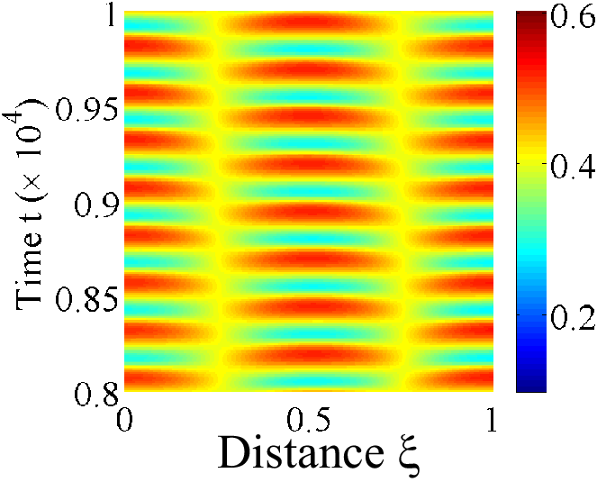
The dynamics of the extended Gray-Scott model with a single diffuser are then obtained as

\displaystyle\begin{array}[]{ll}\displaystyle\frac{\partial x}{\partial t}=-xy^{2}+\eta_{1}y^{3}+\gamma(1-x)\\ \displaystyle\frac{\partial y}{\partial t}=xy^{2}-\eta_{1}y^{3}-k(y-\eta_{2}z)-\gamma y\\ \displaystyle\frac{\partial z}{\partial t}=k(y-\eta_{2}z)-\gamma z+\mu\nabla^{2}z,\end{array}

where $x(\xi,t),y(\xi,t)$ and $z(\xi,t)$ are normalized concentrations of $X,Y$ and $Z$ , respectively. The parameters $(\eta_{1},\eta_{2},k,\gamma)$ and $\mu$ are normalized reaction and diffusion rates, respectively (see [15] for the details).

In what follows, we linearize the system (6) around a homogeneous equilibrium and demonstrate a Type-I Turing pattern predicted by Theorem 2. To this end, we first obtain the three homogeneous equilibria of (6) as

		$\displaystyle(x_{0},y_{0},z_{0})=(1,0,0),$
		$\displaystyle(x_{+},y_{+},z_{+})=\left(\frac{\eta_{1}y_{+}^{3}+\gamma}{y_{+}^{2}+\gamma},\frac{v+\sqrt{w}}{2\left((1+\eta_{1})v+k\right)},\frac{ky_{+}}{v}\right),$
		$\displaystyle(x_{-},y_{-},z_{-})=\left(\frac{\eta_{1}y_{-}^{3}+\gamma}{y_{-}^{2}+\gamma},\frac{v-\sqrt{w}}{2\left((1+\eta_{1})v+k\right)},\frac{ky_{-}}{v}\right),$

where $w:=v^{2}-4\gamma(k+v)\left\{(1+\eta_{1})v+k\right\}$ and $v:=\gamma+k\eta_{2}$ . The Jacobian of (6) at $(x_{*},y_{*},z_{*})$ is then calculated as

\displaystyle\begin{bmatrix}-y_{*}^{2}-\gamma&-2x_{*}y_{*}+3\eta_{1}y_{*}^{2}&0\\ y_{*}^{2}&2x_{*}y_{*}-3\eta_{1}y_{*}^{2}-k-\gamma&k\eta_{2}\\ 0&k&-k\eta_{2}-\gamma\end{bmatrix}.

(20)

Note that we can verify that the equilibrium $(x_{+},y_{+},z_{+})$ can be Turing unstable, whereas $(x_{0},y_{0},z_{0})$ is always stable.

Hence, we hereafter explore Type-I Turing instability around the equilibrium $(x_{+},y_{+},z_{+})$ . Let $\eta_{1}=\eta_{2}=0.1$ . The Jacobian then depends on the two parameters $\gamma$ and $k$ , which are the normalized degradation and production rates of the diffuser $Z$ , respectively. Thus, using Theorem 2, we can specify the parameter region of $(\gamma,k)$ such that the system (6) is Type-I Turing unstable around $(x_{+},y_{+},z_{+})$ as illustrated in Fig. 4.

In order to verify the Type-I Turing unstable condition, we numerically simulated the model (6) for the parameter sets shown in Table 1.

Table 1: The parameter sets for the simulations in Fig. 5

Set	$\gamma$	$k$	$\mu$
A	$1.0\times 10^{-2}$	$6.2\times 10^{-2}$	$1.0\times 10^{-3}$
B	$1.0\times 10^{-2}$	$5.5\times 10^{-2}$	$1.0\times 10^{-3}$

The simulation results are illustrated in Fig. 5 (Right) and Fig. 6 (Right) for the sets $A$ and $B$ , respectively We can verify that the chemical concentration forms the Type-I Turing pattern when the parameter is chosen from the colored region in Fig. 4, while it converges to a spatially homogeneous equilibrium point for the parameters outside the region. Moreover, we can see that the profile of the spatial pattern in Fig. 5 (Right) is the second mode corresponds to the fact that the dominant closed-loop pole is given by $\Sigma_{2}$ (see Fig. 5 (Left)).

The simulations in Figs. 5 and 6 were implemented by the command ‘pdepe’ in MATLAB R2010b. The initial conditions were set as $[x(\xi,0),y(\xi,0),z(\xi,0)]^{T}=\sum_{k=1}^{20}0.01$ $\cos(k\pi\xi)[1,1,1]^{T}$ for both examples.

7 Conclusion

In this paper, we have developed a control theoretic framework to analyze the reaction-diffusion systems with a single diffusible component. We have first shown that the instability analysis of the reaction-diffusion system can be greatly simplified by formulating as a multi-agent dynamical system. This formulation has then allowed us to characterize biologically plausible and implausible Turing instabilities using the root locus of each agent’s dynamics. Thus, using the properties of the root locus, we have proven that the reaction-diffusion systems can exhibit biologically plausible Turing patterns even when there is only one diffusible component. Then, the conditions for the pattern formation have been analytically obtained for systems with three components.

Acknowledgments: This work was supported in part by the Ministry of Education, Culture, Sports, Science and Technology in Japan through Grant-in-Aid for Scientific Research (A) No. 21246067, and Grant-in-Aid for JSPS Fellows No. 23-9203.

References

[1] S. Basu, Y. Gerchman, C. H. Collins, F. H. Arnold, and R. Weiss. A synthetic multicellular system for programmed pattern formation. Nature, 434(7037):1130–1134, 2005.
[2] S. Basu, R. Mehreja, S. Thiberge, M.-T. Chen, and R. Weiss. Spatiotemporal control of gene expression with pulse-generating networks. Proceedings of National Academy of Sciences, 101(17):6355–6360, 2004.
[3] R. F. Curtain and H. J. Swart. An introduction to infinite-dimensional linear systems theory. Springer, 1995.
[4] L. Edelstein-Keshet. Mathematical models in biology. SIAM, 2005.
[5] A. Gierer and H. Meinhardt. A theory of biological pattern formation. Kybernetik, 12(1):30–39, 1972.
[6] S. Hara, H. Tanaka, and T. Iwasaki. Stability analysis of systems with generalized frequency variables. IEEE Transactions on Automatic Control. (to appear).
[7] J. Hsia, W. J. Holtz, D. C. Huang, M. Arcak, and M. M. Maharbiz. A feedback quenched oscillator produces Turing patterning with one diffuser. PLOS Computational Biology, 8(1), 2012. e1002331.
[8] A.J. Koch and H. Meinhardt. Biological pattern formation: from basic mechanisms to complex structures. Reviews of Modern Physics, 66(4):1481–1507, 1994.
[9] S. Kondo and T. Miura. Reaction-diffusion model as a framework for understanding biological pattern formation. Science, 329(5999):1616–1620, 2010.
[10] M. Loose, K. Kruse, and P. Schwille. Protein self-organization: lessons from the min system. Annual Review of Biophysics, 40:315–336, 2011.
[11] M.B. Miller and B.L. Bassler. Quorum sensing in bacteria. Annual Review of Microbiology, 55:165–199, 2001.
[12] J.D. Murray. Mathematical Biology II. Springer, 3rd edition edition, 2003.
[13] H. Tanaka, S. Hara, and T. Iwasaki. LMI stability condition for linear systems with generalized frequency variables. In Proceedings of Asian Control Conference, pages 136–141, 2009.
[14] A. M. Turing. The chemical basis of morphogenesis. Philosophicals Transactions of the Royal Society of London B, 237(641):37–72, 1952.
[15] J. A. Vastano, J. E. Pearson, W. Horsthemke, and H. L. Swinney. Turing patterns in an open reactor. The Journal of Chemical Physics, 88(6175), 1988.

Appendix A Proof of Theorem 2

We prove the theorem by showing equivalent conditions to (i), (ii-a) and (ii-b) in Lemma 3.

It can be verified that $A$ is Hurwitz if and only if

\displaystyle\alpha_{2}>0,~\alpha_{1}\alpha_{2}-\alpha_{0}>0,~\alpha_{0}>0,

(21)

which is equivalent to the condition (i) in Lemma 3.

In what follows, we derive the conditions (II-A) and (II-B) by considering the case where $\tilde{A}$ is Hurwitz and not Hurwitz, respectively. We can easily verify that neither (ii-a) nor (ii-b) of Lemma 3 can be satisfied when $\omega=0$ . Hence, we hereafter show the proof for the case of $\omega\neq 0$ .

Case 1: $\tilde{A}$ is Hurwitz: A necessary condition for $\tilde{A}$ being Hurwitz is

\displaystyle\tilde{\alpha}_{1}>0~\mathrm{and}~\tilde{\alpha}_{0}>0.

(22)

Moreover, $p(\lambda,j\omega)=0$ implies that

		$\displaystyle\mathrm{Re}[p(\lambda,j\omega)]=-\alpha_{2}\omega^{2}+\alpha_{0}+\lambda(-\omega^{2}+\tilde{\alpha}_{0})=0$		(23)
		$\displaystyle\mathrm{Im}[p(\lambda,j\omega)]=-\omega\{\omega^{2}-(\alpha_{1}+\lambda\tilde{\alpha}_{1})\}=0.$		(24)

It follows from (24) that $\omega^{2}=\alpha_{1}+\lambda\tilde{\alpha}_{1}(>0)$ , since $\omega\neq 0$ . We can then eliminate $\omega^{2}$ from (23), and we have the following quadratic equation of $\lambda$ .

\displaystyle\tilde{\alpha}_{1}\lambda^{2}+(\alpha_{1}+\tilde{\alpha}_{1}\alpha_{2}-\tilde{\alpha}_{0})\lambda+\alpha_{1}\alpha_{2}-\alpha_{0}=0.

(25)

Since $\tilde{\alpha}_{1}>0$ and $\alpha_{1}\alpha_{2}-\alpha_{0}>0$ hold from (21) and (22), a necessary and sufficient condition for (25) having a positive real solution is given by the following (C1) and (C2).

(C1) The determinant of (25) is non-negative. That is,

\displaystyle(\alpha_{1}+\tilde{\alpha_{1}}\alpha_{2}-\tilde{\alpha}_{0}^{2})^{2}-4\tilde{\alpha}_{1}(\alpha_{1}\alpha_{2}-\alpha_{0})\geq 0.

(26)

(C2) The coefficient of $\lambda$ in (25) is negative. That is,

\displaystyle\alpha_{1}+\tilde{\alpha}_{1}\alpha_{2}-\tilde{\alpha}_{0}<0.

(27)

Summarizing (26) and (27), we have

\displaystyle\alpha_{1}+\tilde{\alpha}_{1}\alpha_{2}-\tilde{\alpha}_{0}\leq-2\sqrt{\tilde{\alpha}_{1}(\alpha_{1}\alpha_{2}-\alpha_{0})}.

(28)

The condition (II-A) is obtained from (22) and (28).

Case 2: $\tilde{A}$ is not Hurwitz A necessary condition for $\tilde{A}$ not being Hurwitz is

\displaystyle\tilde{\alpha}_{1}\leq 0~\mathrm{or}~\tilde{\alpha}_{0}\leq 0.

(29)

Let $\beta\pm j\gamma~(\beta,\gamma\geq 0)$ denote a pair of eigenvalues of $\tilde{A}$ with the largest real part. Then, $|(\beta+j\gamma)I_{2}-\tilde{A}|=0$ implies

		$\displaystyle\beta^{2}+\tilde{\alpha}_{1}\beta+\tilde{\alpha}_{0}-\gamma^{2}=0$		(30)
		$\displaystyle(2\beta+\tilde{\alpha}_{1})\gamma=0.$		(31)

In what follows, we first show that $p(\lambda,\beta+j\gamma)\neq 0$ for all $\lambda>0$ and $\omega$ when $\gamma=0$ . It follows from $\mathrm{Im}[p(\lambda,\beta+j\omega)]=0$ that

\displaystyle\omega^{2}=3\beta^{2}+2\alpha_{2}\beta+\alpha_{1}+\lambda(2\beta+\tilde{\alpha}_{1}).

(32)

Substituting this into $\mathrm{Re}[p(\lambda,\beta+j\omega)]=0$ yields the following equation of $\lambda$ .

	$\displaystyle(2\beta+\tilde{\alpha}_{1})\lambda^{2}$	$\displaystyle+\{9\beta^{2}+(4\alpha_{2}+3\tilde{\alpha}_{1})\beta+\alpha_{1}+\tilde{\alpha}_{1}\alpha_{2}\}\lambda$
		$\displaystyle+\{8\beta^{3}+8\alpha_{2}\beta^{2}+2(\alpha_{1}+\alpha_{2}^{2})\beta+(\alpha_{1}\alpha_{2}-\alpha_{0})\}=0.$		(33)

It should be noted that the coefficient of $\lambda^{2}$ is non-negative, or $2\beta+\tilde{\alpha}_{1}\geq 0$ , since $\beta$ is the largest real root of $s^{2}+\tilde{\alpha}_{1}s+\tilde{\alpha}_{0}=0$ from the definition. Moreover, (21) and (29) imply that the coefficient of $\lambda$ and the constant terms of (33) are positive as well. Thus, $p(\lambda,\beta+j\gamma)\neq 0$ for all $\lambda>0$ and $\omega$ when $\gamma=0$ .

When $\gamma\neq 0$ , the determinant of $|sI_{2}-\tilde{A}|=0$ is negative, thus we have

\displaystyle\tilde{\alpha}_{1}^{2}-4\tilde{\alpha}_{0}<0.

(34)

Moreover, $\mathrm{Im}[p(\lambda,\beta+j\omega)]=0$ implies

\displaystyle\omega^{2}=3\beta^{2}+2\alpha_{2}\beta+\alpha_{1}.

(35)

Substituting this into $\mathrm{Re}[p(\lambda,\beta+j\omega)]=0$ yields

\displaystyle\{\gamma^{2}-(3\beta^{2}+2\alpha_{2}\beta+\alpha_{1})\}\lambda-\{8\beta^{3}+8\alpha_{2}\beta^{2}+2(\alpha_{1}+\alpha_{2}^{2})\beta+(\alpha_{1}\alpha_{2}-\alpha_{0})\}=0.

(36)

Note that the constant term of (36) is negative because of (21) and $\beta>0$ . Thus, (36) has a positive real root if and only if

\displaystyle\gamma^{2}-(3\beta^{2}+2\alpha_{2}\beta+\alpha_{1})>0.

(37)

The condition (II-B) is obtained from (29), (30), (31), (34) and (37). $\hfill\Box$