Achieving the Optimal Steaming Capacity and Delay Using Random Regular Digraphs in P2P NetworksThanks: The research reported here was funded by NSF grant CNS-0964081 and AFOSR MURI FA 9550-10-1-0573.

The peer-pairing algorithm constructs $M$ independent 1-regular digraphs. The topology of the P2P system is the union of these $M$ digraphs. For the theoretical results in the paper, $M$ can be as little as two, but can be larger for robustness reasons in a practical implementation. Since every peer has one incoming edge and one outgoing edge in a 1-regular digraph, it has $M$ incoming edges and $M$ outgoing edges, and thus the resulting topology is a $M$-regular digraph. We index the $M$ incoming edges and the $M$ outgoing edges from 1 to $M$, respectively. We call the peer at the other end of the $m$-th incoming edge of peer $v$ the $m$-th parent of peer $v$ and denote by $p_{m}(v)$. Similarly, we call the peer in the other end of the $m$-th outgoing edge of peer $v$ the $m$-th child and denote by $c_{m}(v)$. Peer $v$ receives chunks from the parents through its incoming edges and send chunks to the children through its outgoing edges.

We present the peer pairing algorithm, i.e., the algorithm used by every peer $v$ to find its parents and children, in Algorithm 1. At a given time instant, let $L_{m}=(V,E_{m})$ denote a digraph with all peers and their $m$-th outgoing edges, i.e., $E_{m}=\{(v,c_{m}(v))|v\in V\}$. We call this graph layer $m$ for $m=1,2,\cdots,M$. The network topology is then the graph formed by the superposition of all the layers. A layer begins with an initial peer, the source, with a loop. When a new peer $v$ joins, it chooses an edge from the layer and breaks into the middle of the edge or creates a loop. When an existing peer leaves, its incoming edge and outgoing edge in the layer are connected directly. Hence, at any given movement, a layer must be a 1-regular digraph where every peer has only one incoming edge and one outgoing edge in the layer.

Let $\Pi(V)$ be the set of all possible 1-regular digraphs that can be made of peers in $V$. A simple way to construct a 1-regular digraph is by a permutation of the peers. For $V=\{1,\cdots,N\}$, let $(v^{(1)},v^{(2)},\cdots,v^{(N)})$ be a permutation of $(1,2,\cdots,N)$. If we draw an edge from $i$ to $v^{(i)}$ for each $i$, all peers will have exactly one incoming edge and one outgoing edge. Hence, the resulting graph becomes 1-regular digraph. Since the number of all possible permutations is $N!$, we can make $N!$ different 1-regular digraphs using $N$ peers, i.e., $\Pi(V)=|V|!$. The following result shows that each layer is one of these graphs equally likely and is independent of other layers:

Note the key difference of the peer-pairing algorithm in this paper from that in our previous paper [6]. In the previous algorithm, the name server first chooses $(w_{1},\cdots,w_{M})$ from $V$ and then adds new peer $v$ to $V$, which eliminates the probability of having $w_{m}=v$. Hence, new peers do not create a loop and thus each layer is a Hamiltonian cycle, which is a special case of regular-1 digraphs (see [6] for the details). In contrast, new peers in this paper may create loops in a layer and thus a layer could have multiple cycles or loops.

Although the algorithm constructs and maintains the network topology in a distributed fashion, it still needs a name server that provides a new peer with the IP addresses of $M$ existing peers. The server performing this minimal function is called a tracker, and is commonly used in most P2P networks. Under our algorithm, the name server only knows the set of existing peers and does not need to know the connections between them. Further, the set of existing peers could be outdated, in which case new peers contact the name server again if some of the retrieved peers are not reachable. Lastly, our algorithm is scalable because every peer exchanges chunks with $2M$ peers, regardless of the network size.

We next present the chunk-exchange algorithm that disseminates chunks over the network topology constructed by the aforementioned peer-pairing algorithm. We assume that the network is time-slotted and the source generates up to $M$ unit-size chunks from real-time video contents during every time slot. We also assume that every peer can upload at most one chunk through every outgoing edge. Since every peer has $M$ outgoing edges, we are assuming that every peer has an upload bandwidth of $M$. Since every peer has $M$ incoming edges, the download bandwidth required for our algorithm is also $M$. When a peer receives a chunk at a give time slot, this peer can transmit the chunk from the next time slot.

For chunk dissemination, we split the chunks into $M$ flows, named flow 1, flow 2, …, flow $M$. When the source generates $M$ or less chunks at a given time slot, it assigns the $M$ flows to the chunks uniquely. We call the chunk assigned flow-$f$ flow-$f$ chunks. Every peer also assigns $M$ flows to its $M$ incoming edges uniquely. As a result, every edge is assigned one of the $M$ flows. We call edges assigned flow-$f$ flow-$f$ edges. Let $f_{m}(v)$ be the flow assigned to the $m$-th incoming edge of peer $v$. Every peer $v$ determines $f_{m}(v)$ for each $m$ using the flow-assignment algorithm in Algorithm 2. Under the flow-assignment algorithm, every peer assigns $M$ flows to all the incoming edges uniquely while a peer may have two or more outgoing edges with the same flow.

Under our chunk dissemination algorithm, each chunk from a flow is transmitted through the same-flow edges. Specifically, we assume that every peer maintains a FIFO (First-In-First-Out) queue for each outgoing edge. When a peer receives a flow-$f$ chunk from a parent or the source peer generates a flow-$f$ chunk, the peer adds the chunk to the queues associated with the flow-$f$ outgoing edges. At the beginning of a time slot, every peer takes the oldest chunk from each queue and transmits the chunk through the outgoing edge associated with the queue.

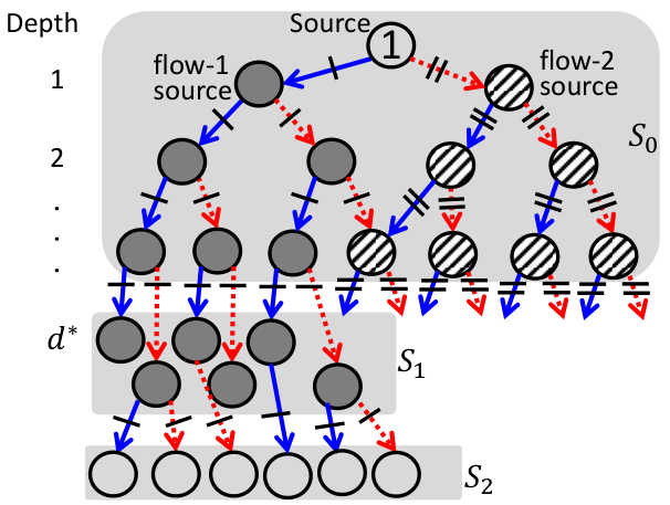
Our chunk dissemination algorithm called RFA is presented in Algorithm 2. We next describe how the RFA algorithm works. See Fig. 1 that shows flow assignment for the simplest case $M=2$. Under the algorithm, the $m$-th child of the source assigns flow-$m$ to its $m$ incoming edge from the source. Hence, the source sends flow-$m$ chunks through its $m$-th outgoing edge. Since the $m$-th child is the peer that directly receives flow-$m$ chunks from the source, we call it flow-$m$ source. The $m$-th child then sets its distance to be 1, i.e., $d(v)=1$, and $\chi(v)=m$. We call the peers with $d(v)\leq d^{*}$ and $\chi(v)=m$ flow-m peers because flow-m chunks are disseminated through these peers. The children $v$ of the flow-1 source will choose $d(v)=2$, and $\chi(v)=1$. $d(v)=2$ means the distance of peer $v$ from the source is 2, and $\chi(v)=1$ implies that peer $v$ is closer to the flow-1 source than the flow-2 source. This holds for $d(v)=1,2,\cdots,d^{*}$, for an appropriately chosen $d^{*}$ which will be described later. Note that if a peer has the same distance from the flow-1 source or the flow-2 source and has two parents with different main flows (as the forth peer in depth 3 in Fig. 1) it decides its main flow randomly and then the children will be affected by the decision. Beyond depth $d^{*}$, peers assign flow 1 to one of its incoming edges randomly regardless of the depth or the main flow of its parents.

In this subsection, we first consider the number of peers in each depth $d\leq d^{*}$. Let $\mathcal{N}_{d}$ be the peers $v$ in depth $d$, i.e., $d(v)=d$, and let $N_{d}\triangleq|\mathcal{N}_{d}|.$ For simplicity, we also define $\mathcal{N}_{\leq d}\triangleq\cup_{h=0}^{d}\mathcal{N}_{d}$ and $\mathcal{N}_{>d}\triangleq\mathcal{N}_{\leq d}^{C}$ to be the set of peers that are within and beyond, respectively, depth $d$. Let $N_{\leq d}=|\mathcal{N}_{\leq d}|$ and $N_{>d}=|\mathcal{N}_{>d}|$.

Recall that each layer constructed by our peer-pairing algorithm is a random 1-regular digraph uniformly distributed among all possible 1-regular digraphs, and an equivalent graph can be constructed by random permutation. Specifically, for given peers and no initial edges, we pick the first peer arbitrarily and draw an edge from the peer to a peer randomly chosen among the peers that do not have an incoming edge. Initially, all the peers can be a candidate because there is no edge drawn. We then pick the second peer among the peers that do not have an outgoing edge and draw an edge from the peer to a peer randomly chosen among the peers that do not have an incoming edge. If we draw $N$ edges repeating this method, the resulting graph becomes a random 1-regular digraph, which has the same distribution as an each layer.

Using this edge drawing procedure with random permutation, we find the distribution of the number $N_{d}$ of peers in each depth $d$. Define $\mathcal{G}(d)$ to be the graph of peers within depth $d+1$ and the outgoing edges from the peers within depth $d$. See the example in Fig. 3(a). Note that when $\mathcal{G}(d)$ is given, $N_{0},N_{1},\cdots,N_{d+1}$, $N_{\leq d+1}$, and $N_{>d+1}$ are determined. In the example in Fig. 3(a), conditioned on $\mathcal{G}(1)$, i.e., conditioned on that the network topology up to depth $2$ is given $\mathcal{G}(1)$, we first draw layer-1 edges from the peers in depth $2$, i.e., $\mathcal{N}_{2}$. When we draw a layer-1 outgoing edge from the first peer in depth 2, there is one layer-1 edge from each peer in $\mathcal{N}_{\leq 1}$. This means that there are $N_{\leq 1}$ peers that have a layer-1 incoming edge. Hence, the new edge can be drawn to one of the remaining $N_{>1}$ peers. If we draw an edge to one of the $N_{>2}$ peers that are not within depth 2, the peer will be added to $\mathcal{N}_{3}$ as shown in Fig. 3(b). If we draw an edge to one of the peers within depth $2$ (see the fourth peer in $\mathcal{N}_{2}$), the peer will not be added to $\mathcal{N}_{3}$. Hence, drawing layer-1 edges from the peers in $\mathcal{N}_{2}$ can be seen as the experiment where the peers in $\mathcal{N}_{2}$ choose one peer without repetition among $N_{>1}$ peers and a peer chosen from $\mathcal{N}_{>2}$ is considered to be a success.

Define $\mathcal{N}_{d}^{\prime}$ to be the set of the peers in depth $d$ that are connected from the peers in depth $d-1$ through layer-1 edges. Let $N_{d}^{\prime}=|\mathcal{N}_{d}^{\prime}|$. In the example, $N_{3}^{\prime}$ is equivalent to the number of red balls among $N_{2}$ balls drawn from a jar containing $N_{>1}$ balls including $N_{>2}$ red balls without replacing balls. The number of the red balls in this example is known to be a hyper geometric random variable with parameters $(N_{>1},N_{>2},N_{2})$. In general, conditioned on $N_{0},N_{1},\cdots,N_{d}$, $N_{d+1}^{\prime}$ is a hyper geometric random variable with $(N_{>d-1},N_{>d},N_{d})$ which has the following mean:

After drawing the layer-1 edges from the peers in depth 2, we next draw layer-2 edges from the same peers. Let $\mathcal{N}_{d}^{\prime\prime}$ be the set of the peers in depth $d$ that are connected from the peers in depth $d-1$ only through layer-2 edges. Let $N_{d}^{\prime\prime}=|\mathcal{N}_{d}^{\prime\prime}|$. Since there is one layer-2 edge from each peers in $\mathcal{N}_{\leq 1}$, there are $N_{>1}$ peers that we can draw layer-2 edges to. If we drawn an edge from a peer in $\mathcal{N}_{2}$ to a peer not in $\mathcal{N}_{\leq 2}\cup\mathcal{N}_{3}^{\prime}$, the peer is newly added to $\mathcal{N}_{3}^{\prime\prime}$, which will be considered to be a success. Otherwise, $\mathcal{N}_{3}^{\prime\prime}$ is not incremented. (See that the third peer in $\mathcal{N}_{3}$ in Fig 3(c) does not belong to $\mathcal{N}_{3}^{\prime\prime}$, but $\mathcal{N}_{3}^{\prime}$.). Hence, drawing layer-2 edges from $\mathcal{N}_{2}$ can be seen as the experiment that $N_{2}$ peers are drawn without replacement from a jar containing $N_{>1}$ balls including $N_{>2}$ red balls. Hence, $\mathcal{N}_{3}^{\prime\prime}$ is equivalent to the number of the red drawn balls in the experiment, which is a hyper geometric random variable with $(N_{>1},N_{>2}-N_{3}^{\prime},N_{2})$. In general, $N_{d+1}^{\prime\prime}$ is a hyper geometric random variable with $(N_{>d-1},N_{>d}-N_{d+1}^{\prime},N_{d})$, which has the following mean:

Combining (1) and (2), the mean of the number of the peers in depth $d+1$ is given by

From (3), when $N_{\leq d}$ is small, i.e., the number of the peers within depth $d$ is small compared to $N$, the number $N_{d}$ of the peers in depth $d$ is expected to double approximately as $d$ increases. We want to show that this phenomenon continues to hold for all $d\leq d^{*}$, which requires a stronger concentration result.

Using a property of a hyper geometric distribution, we derive the concentration result for pretty small $N_{d}$:

The proof is provided in Appendix A in our online technical report [25]. The proof is provided in Appendix -A. The lemma implies that the arborescence is 2-ary up to depth $\frac{1}{2}(1-\epsilon)\log_{2}N$ with high probability. However, this concentration result does not hold for a higher depth. We can derive another concentration result for this case:

The detailed proof is provided in Appendix B in [25]. The detailed proof is provided in Appendix -B.

The proof is provided in Appendix C in [25]. The proof is provided in Appendix -C.

Proposition 3 implies that the number of the peers in each depth $d$ doubles up to depth $d_{1}$ with probability 1. For depth $d_{1}<d\leq d^{*}$, the number of the peers in depth $d$ increases by $2\phi_{d}$ times with high probability. Since $2\phi_{d}$ in this case is nearly 2, the arborescence up to depth $d^{*}$ is nearly a binary tree with high probability.

We next consider the number of flow-1 peers in each depth. Recall that under the RFA algorithm, every peer $v$ within depth $d^{*}$ determines its main flow $\xi(v)$. In Fig. 1, flow-1 peers are shown in gray. Let $\mathcal{X}_{d}$ be the set of gray peers in depth $d$, and $X_{d}=|\mathcal{X}_{d}|$. By symmetry, the expected number of flow-1 peers in depth $d$ must be a half of the peers in the same depth, i.e., $X_{d}=E[N_{d}/2]$. The next proposition shows that when the arborescence up to depth $d^{*}$ is nearly a binary tree, the portion of flow-1 peers in each depth is concentrated on a half, $X_{d}/N_{d}\approx 1/2$:

The proof is provided in Appendix D in [25]. The proof is provided in Appendix -D.

In this subsection, we have shown that the arborescence up to $d^{*}$ is nearly a binary tree and a half of the peers in each depth are flow-1 peers with high probability. Since every flow-1 peer in the arborescence is connected from the source only with $d^{*}$ or less flow-1 edges, the flow-1 peers in the arborescence are connected from the source in flow graph 1 within $d^{*}$ hops. This means that the flow-1 peers can receive flow-1 chunks with delay $d^{*}=O(\log N)$. In the next subsection, we will consider how these chunks can be disseminated to the peers beyond $d^{*}$ through the flow-1 peers in depth $d^{*}$.

We now show that the maximum distance from the flow-1 peers within depth $d^{*}$ to peers $v$ with $d>d^{*}$ in flow graph 1.

Let $\mathcal{S}_{0}$ be the set of the peers within depth $d^{*}-1$ as shown in Fig. 1, i.e., $\mathcal{S}_{0}=\{v\in V\;|\;d(v)<d^{*}\}.$ Let $\mathcal{S}_{1}$ be the set of the flow-1 peers in depth $d^{*}$, i.e., $\mathcal{S}_{1}=\{v\in V\;|\;d(v)=d^{*},\chi(v)=1\}.$ We have shown that the number of the peers in depth $d^{*}$ is larger than $\frac{N}{\log^{c}N}$ with high probability in Proposition 3 and a half of them are flow-1 peers that belong to $\mathcal{S}_{1}$ in Proposition 4 with high probability. We then iteratively define $\mathcal{S}_{h}\subset V$ for $h>1$ and $m=1,2$ as follows:

In other words, $\mathcal{S}_{h}$ is the set of the peers not in $\cup_{l=0}^{h-1}\mathcal{S}_{l}$ that are connected from the peers in $\mathcal{S}_{h-1}$ through flow-1 incoming edges. (See the example in Fig 1. We also define $\mathcal{S}_{\leq h}\triangleq\cup_{d=0}^{h}\mathcal{S}_{d}$ and $\mathcal{S}_{>h}\triangleq\mathcal{S}_{\leq h}^{C}$. For simplicity, let $S_{h}\triangleq|\mathcal{S}_{h}|$, $S_{\leq h}\triangleq|\mathcal{S}_{\leq h}|$, and $S_{>h}\triangleq|\mathcal{S}_{>h}|$.

Since the peers in $\mathcal{S}_{h}$ are connected from the peers in $\mathcal{S}_{h-1}$ through flow-1 edges, the distance from the peers in $\mathcal{S}_{0}$ to the peers in $\mathcal{S}_{h}$ in flow graph 1 is exactly $h$. Since the peers in $\mathcal{S}_{1}$ are $d^{*}$ hops away from the source in flow graph 1, the peers in $\mathcal{S}_{h}$ must be $d^{*}+h$ hops from the source in flow graph 1. Therefore, our goal in this subsection is to show that $\mathcal{S}_{\leq O(\log N)}$ covers almost all peers in the network with high probability.

While we have used edge expansion in the previous subsection, we use the contraction of the number of remaining peers. Specifically, define contraction ratio $\gamma_{h}$ as

From the result in the previous subsection, the initial contraction ratio $\gamma_{1}$ is upper bounded by

The contraction ratio can be interpreted as the fraction by which the number of peers not within $h$ hops from the source in flow graph 1 decreases at each $h$. We will first show that the sequence of $\gamma_{1},\gamma_{2},\cdots,$ is a martingale in Proposition 5, and then establish the following concentration result:

This concentration result leads to the following:

Taking $h=\log N$, the R.H.S. of (4) approaches $N/\exp({\log^{1-c}N})$, which converges to zero as $N$ increases. This implies that in a large network, only $o(1)$ fraction of peers do not belong to $\mathcal{S}_{\leq\log N}$, hence all the remaining peers beyond depth $d^{*}$ are within $d^{*}+\log N$ hops from the source in flow graph 1.

We consider the distribution of $S_{1},S_{2},\cdots.$ using the example in Fig. 1. Suppose the outgoing edges from the peers in $\mathcal{S}_{0}$ and $\mathcal{S}_{1}$ are given as in the figure, and thus $\mathcal{S}_{2}$ is also determined. We find the distribution of $S_{3}$ by drawing random edges from $\mathcal{S}_{2}$. Recall that each peer beyond depth $d^{*}$ assigns flow 1 to one of its incoming edges uniformly at random. Among the peers in $\mathcal{S}_{>2}$, let $\mathcal{S}_{>2,m}$ be the set of the peers beyond depth $d^{*}$ that assign flow 1 to its $m$-th incoming edge, i.e.,

and let $S_{>2,m}=|\mathcal{S}_{>2,m}|$. When we draw a layer-1 edge from a peer in $\mathcal{S}_{2}$, there is a layer-1 edge outgoing from every peer in $\mathcal{S}_{\leq 1}$. Hence, there are $S_{>1}$ peers that we can draw the layer-1 edge to. Among these peers, if we draw the edge to a peer in $\cap S_{>2,1}$, i.e., a peer that assigned flow 1 to its first incoming edge, the peer in $S_{2}$ and the chosen peer are connected through flow-1 edge, and thus the chosen peer will be added to $\mathcal{S}_{3}$. If we draw the edge to a peer $S_{>2,2}$ that assigned flow 2 to its layer-2 incoming edge, the peer will not be added to $\mathcal{S}_{3}$ because the chosen peer is connected through flow-2 edge. Hence, there are $S_{>1}$ peers that we can draw layer-1 edges from $S_{1}$ to and drawing to a peer in $S_{>2,1}$ will be considered to be a success. Hence, $S_{3,1}$ is a hyper geometric random variable with parameters $(S_{>1},S_{>2,1},S_{2})$. By symmetry, $S_{3,2}$ is a hyper geometric random variable with $(S_{>1},S_{>2,2},S_{2})$. In general, we can conclude the following:

Using the properties of hyper geometric random variables, we can derive the following martingale property:

The proof is provided in Appendix E in [25]. The proof is provided in Appendix -E.

The result implies that the expected ratio $S_{>d}/S_{>d-1}$ of the remaining peers at each hop $d$ remains $\gamma_{1}$ as $d$ increases. We extend the martingale result to the following stronger concentration result:

The proof is provided in Appendix F in [25]. The proof is provided in Appendix -F.

From Proposition 6, the contraction ratio only increases slightly with the number of hops with high probability. Hence, this concentration result holds for $\gamma_{1},\gamma_{2},\cdots,\gamma_{h}$, the numbers of remaining peers, $S_{>1},S_{>2},\cdots,S_{>h}$, decrease exponentially. In the next proposition, we show that $S_{>h}$ becomes smaller than $N/\exp(\log^{1-c}N)$ before $h<\log N$:

The proof is provided in Appendix G in [25]. The proof is provided in Appendix -G.

In the previous section, we have shown that flow-1 peers in $\mathcal{S}_{0}$ are within $d^{*}=O(\log N)$ hops away from the source in flow graph 1. Here, we have shown that ($1-o(1)$) fraction of peers beyond depth $d^{*}$ are within $\log N$ hops away from the flow-1 peers in $S_{0}$ in flow graph 1. Hence, all the aforementioned peers are within $O(\log N)$ hops in flow graph 1. In the next subsection, we show that the flow-2 peers in $\mathcal{S}_{0}$ are also connected in flow graph 1 from the source within $O(\log N)$ hops.

Previously, we have shown that all the flow-1 peers within depth $d^{*}$ and almost all peers below depth $d^{*}$ are connected from the source in flow graph 1 with high probability. In this subsection, we consider how the remaining peers, the flow-2 peers within depth $d^{*}$, are connected in flow graph 1. By showing that most of them are connected from the peers below depth $d^{*}$ with a flow-1 incoming edge with high probability, we show that the flow-2 peers are also connected in flow graph 1 within $O(\log N)$ hops.

We provide the basic idea of the proof and refer to our online technical report for the details. As we can see in Fig. 1, all the outgoing edges from flow-2 peers in $\mathcal{S}_{0}$ are all assigned flow 2. Recall that every peer has one flow-1 incoming edge under the RFA algorithm. Hence, all the flow-1 edges incoming to the flow-2 peers must come from the flow-1 peers in $\mathcal{S}_{0}$ or from the peers below depth $d^{*}$. However, we have shown in Proposition 3 that $N_{d}>2(1-\phi_{d})N_{d-1}$ with high probability. This means that the number of the flow-1 edges that begin at the flow-1 peers in depth $d-1$ and end at flow-2 peers within depth $d$ and the flow-2 edges that begin at flow-2 peers in depth $d-1$ and end at flow-2 peers within depth $d$ is no larger than $2\phi N_{d-1}$, which is a small fraction compared to all the edges outgoing from the peers in depth $2$. In Fig. 1, the second edge outgoing from the second peer in depth 2 corresponds to this case. Overall, only a small fraction $2\max\phi_{d}$ of edges beginning at the peers within depth $d^{*}$ end at the peers with different flows. Hence, most flow-1 incoming edges of the flow-2 peers within depth $d^{*}$ come from the peers below depth $d^{*}$, most of which are $d^{*}+h^{*}$ hops away from the source in flow graph 1. Hence, we can conclude that almost all flow-2 peers in depth 2 are within $d^{*}+h^{*}+1$ hops away from the source in flow graph 1, where $d^{*}+h^{*}+1=O(\log N)$.

To satisfy $N_{d}=2N_{d-1}$, we must have $N_{d}^{\prime}=N_{d}^{\prime\prime}=N_{d-1}$. We first find the probability that the $N_{trial}$ balls drawn without replacement from a jar containing $N_{all}$ balls including $N_{red}$ red balls are all red. Since the number $X$ of the red balls among the drawn balls is a hyper geometric random variable with ($N_{all}$, $N_{red}$, $N_{trial}$), we can derive the probability using [26, Prob. (c), page 11]:

The second term can be seen as the number of possible ways to pick $N_{trial}$ red balls over the number of possible ways to pick any $N_{trial}$ balls.

Recall that $N_{d}^{\prime}$ is a hyper geometric random variable with ($N_{>d-2}$, $N_{>d-1}$, $N_{d-1}$). Applying $N_{d}^{\prime}$ to (5), we have the following bound: conditioned on $N_{0},\cdots,N_{d-1}$,

Conditioned on $N_{d}^{\prime}=N_{d-1}$, $N_{d}^{\prime\prime}$ is also a hyper geometric random variable with ($N_{>d-2}$, $N_{>d-1}-N_{d-1}$, $N_{d-1}$). Hence, we also have

Combining both, we conclude the following bound: conditioned on $N_{0},\cdots,N_{d-1}$,

Note that if $N_{h}=2N_{h-1}$ for all $0<h\leq d$, it is easy to see that $N_{h}=2^{h}$ and $N_{\leq h}=2^{h+1}-1$ for all $h\leq d$. Using this, we derive the following probability:

which is the result of this lemma.

Since $N_{d+1}^{\prime}$ is a hyper geometric random variable with $(N_{>d-1},N_{>d},N_{d})$, the following concentration result holds [26, page 98]:

where $t=(1-\frac{N_{d}}{N_{>d-1}}-\phi)N_{d}\geq\sigma_{d}N_{d}$. From (1), we can infer that if $N_{d+1}^{\prime}<\phi N_{d}$, then $|N_{d+1}^{\prime}-E[N_{d+1}^{\prime}]|>t$. Hence, we have

References

- [1] J. H. Kim and N. C. Wormald, “Random matchings which induce hamilton cycles and hamiltonian decompositions of random regular graphs,” Journal of Combinatorial Theory, Series B, vol. 81, no. 1, pp. 20 – 44, 2001. [Online]. Available: http://www.sciencedirect.com/science/article/pii/S0095895600919919
- [2] C. Law and K.-Y. Siu, “Distributed construction of random expander networks,” in Proceedings of IEEE INFOCOM, vol. 3, April 2003, pp. 2133 – 2143 vol.3.
- [3] Y.-J. Chu and T.-H. Liu, “On the shortest arborescence of a directed graph,” Science Sinica, vol. 14, pp. 1396–1400, 1965.
- [4] J. Edmonds, “Edge-disjoint branchings,” Combinatorial Algorithms, pp. pp. 91–96, 1972.
- [5] R. E. Tarjan, “Finding optimum branchings,” Networks, vol. 7, no. 1, pp. 25–35, 1977. [Online]. Available: http://dx.doi.org/10.1002/net.3230070103
- [6] J. Kim and R. Srikant, “Real-time peer-to-peer streaming over multiple random hamiltonian cycles,” IEEE Transactions on Information Theory, to appear. [Online]. Available: http://arxiv.org/abs/1207.3110
- [7] J. Kim, C. Jiang, and R. Srikant, “A lightweight low-delay streaming protocol for dynamic peer-to-peer networks,” UIUC, Tech. Rep., 2013. [Online]. Available: http://www.ifp.illinois.edu/~joohwan/Kim13tech3.pdf
- [8] R. Kumar, Y. Liu, and K. Ross, “Stochastic Fluid Theory for P2P Streaming Systems,” in Proceedings of IEEE INFOCOM, Anchorage, AL, April 2007.
- [9] J. Mundinger, R. Weber, and G. Weiss, “Optimal scheduling of peer-to-peer file dissemination,” J. of Scheduling, vol. 11, pp. 105–120, April 2008. [Online]. Available: http://dl.acm.org/citation.cfm?id=1349638.1349650
- [10] J. Li, P. A. Chou, and C. Zhang, “Mutualcast: an efficient mechanism for one-to-many content distribution,” in Proceedings of ACM SIGCOMM, Beijing, China, April 2005.
- [11] S. Liu, R. Zhang-Shen, W. Jiang, J. Rexford, and M. Chiang, “Performance bounds for peer-assisted live streaming,” in Proceedings of ACM SIGMETRICS, Annapolis, MD, 2008, pp. 313–324.
- [12] S. Liu, M. Chen, S. Sengupta, M. Chiang, J. Li, and P. A. Chou, “P2p streaming capacity under node degree bound,” in Proceedings of IEEE ICDCS, 2010, pp. 587–598.
- [13] A. M. Frieze and G. R. Grimmett, “The shortest-path problem for graphs with random arc-lengths,” Discrete Applied Mathematics, vol. 10, no. 1, pp. 57 – 77, 1985.
- [14] L. Massoulie, A. Twigg, C. Gkantsidis, and P. Rodriguez, “Randomized decentralized broadcasting algorithms,” in Proceedings of IEEE INFOCOM, 2007, pp. 1073–1081.
- [15] S. Sanghavi, B. Hajek, and L. Massoulie, “Gossiping with multiple messages,” in In IEEE Transactions on Information Theory, 2007, pp. 4640–4654.
- [16] T. Bonald, L. Massoulie, F. Mathieu, D. Perino, and A. Twigg, “Epidemic Live Streaming: Optimal Performance Trade-Offs,” in Proceedings of ACM SIGMETRICS, Annapolis, MD, June 2008.
- [17] C. Zhao, X. Lin, and C. Wu, “The streaming capacity of sparsely-connected p2p systems with distributed control.” in INFOCOM. IEEE, 2011, pp. 1449–1457.
- [18] X. Zhang, J. Liu, B. Li, and Y.-S. Yum, “Coolstreaming/donet: a data-driven overlay network for peer-to-peer live media streaming,” in Proceedings of IEEE INFOCOM, vol. 3, March 2005, pp. 2102 – 2111.
- [19] Y. Zhou, D. M. Chiu, and J. Lui, “A simple model for analyzing p2p streaming protocols,” in Network Protocols, 2007. ICNP 2007. IEEE International Conference on, 2007, pp. 226 –235.
- [20] S. Shakkottai, R. Srikant, and L. Ying, “The asymptotic behavior of minimum buffer size requirements in large p2p streaming networks,” Selected Areas in Communications, IEEE Journal on, vol. 29, no. 5, pp. 928 –937, may 2011.
- [21] J. Liu, S. G. Rao, B. Li, and H. Zhang, “Opportunities and challenges of peer-to-peer internet video broadcast,” in Proceedings of the IEEE, Special Issue on Recent Advances in Distributed Multimedia Communications, 2007.
- [22] D. Ren, Y.-T. Li, and S.-H. Chan, “On reducing mesh delay for peer-to-peer live streaming,” in INFOCOM 2008. The 27th Conference on Computer Communications. IEEE, 2008, pp. 1058–1066.
- [23] G. Dan and V. Fodor, “Delay asymptotics and scalability for peer-to-peer live streaming,” Parallel and Distributed Systems, IEEE Transactions on, vol. 20, no. 10, pp. 1499–1511, 2009.
- [24] S. Traverso, L. Abeni, R. Birke, C. Kiraly, E. Leonardi, R. Lo Cigno, and M. Mellia, “Experimental comparison of neighborhood filtering strategies in unstructured p2p-tv systems,” in Peer-to-Peer Computing (P2P), 2012 IEEE 12th International Conference on, 2012, pp. 13–24.
- [25] J. Kim and R. Srikant, “Achieving the optimal steaming capacity and delay using random regular digraphs in p2p networks,” UIUC, Tech. Rep., 2013. [Online]. Available: http://www.ifp.illinois.edu/~joohwan/Kim13tech2.pdf
- [26] D. Dubhashi and A. Panconesi, Concentration of Measure for the Analysis of Randomized Algorithms, 1st ed. New York, NY, USA: Cambridge University Press, 2009.