P. G. Constantine, E. T. Phipps, T. M. WildeyUQ for network multiphysics systems
Sandia National Laboratories, Optimization and Uncertainty Quantification Department, PO Box 5800, MS-1318, Albuquerque, NM 87185.
Efficient uncertainty propagation for network multiphysics systems
Abstract
We consider a multiphysics system with multiple component models coupled together through network coupling interfaces, i.e., a handful of scalars. If each component model contains uncertainties represented by a set of parameters, a straightfoward uncertainty quantification (UQ) study would collect all uncertainties into a single set and treat the multiphysics model as a black box. Such an approach ignores the rich structure of the multiphysics system, and the combined space of uncertainties can have a large dimension that prohibits the use of polynomial surrogate models. We propose an intrusive methodology that exploits the structure of the network coupled multiphysics system to efficiently construct a polynomial surrogate of the model output as a function of uncertain inputs. Using a nonlinear elimination strategy, we treat the solution as a composite function: the model outputs are functions of the coupling terms which are functions of the uncertain parameters. The composite structure allows us to construct and employ a reduced polynomial basis that depends on the coupling terms; the basis can be constructed with many fewer system solves than the naive approach, which results in substantial computational savings. We demonstrate the method on an idealized model of a nuclear reactor.
keywords
uncertainty quantification, multiphysics systems, network coupling, polynomial chaos, stochastic Galerkin, reduced quadrature1 Introduction
In the growing field of uncertainty quantification (UQ), researchers seek to increase the credibility of computer simulations by modeling uncertainties in the system inputs and measuring the resulting uncertainties in simulation outputs. A common setup in UQ includes a physical model – typically a partial differential equation (PDE) – with imprecisely characterized input data, e.g., boundary conditions or material properties. The uncertainty in the inputs is modeled by a set of random variables, which induces variability in the solution of the physical model. The PDE solution is treated as a map from model inputs to model outputs, and one can use Monte Carlo methods to approximate statistics like moments or density functions of the output. However, if the PDE solution is computationally expensive, then it may not be possible to compute an ensemble with sufficiently many members for accurate statistics. In this case, a cheaper surrogate response surface can be trained on a few input/output evaluations, which is subsequently sampled to approximate statistics.
The procedure just described is blind to the details of the physical model; it only needs a well-posed map from inputs to outputs. This blindness is particularly unsatisfying when the physical model contains rich structure. For example, many models in engineering – e.g., fluid-structure interaction or turbulent combustion – include multiple physical components that are coupled through interfaces. Such multiphysics models are almost always computationally expensive, and thus UQ studies require surrogate response surfaces. However, the process of collecting the uncertainties from each component model into one set of inputs may yield a high-dimensional input space where accurate response surfaces are infeasible. Response surfaces based on polynomial approximation [1, 2] become exponentially more expensive to construct as the dimension of the input space increases; this is related to the so-called curse of dimensionality.
In this work, we propose a method for efficiently constructing accurate polynomial surrogates of the input/ouput map that exploits the coupled structure of a multiphysics model. Tackling all types of multiphysics models is unreasonable, so we focus on a model problem with particular characterstics. We will develop the method in the context of a steady, spatially discretized model with two physical components. These components are coupled through a handful of scalar coupling terms, which we refer to as network coupling. Each physical component contains its own set of parameters representing uncertain inputs, but the nature of the coupling is assumed to be known precisely.
We can summarize our proposed method as follows. We first transform the network coupled multiphysics model to a low dimensional system with a nonlinear elimination method; this approach defines the coupling terms as implicit functions of solutions of the physical component models. We then posit a polynomial model of the coupling terms as functions of the random inputs that follows the formalism of polynomial chaos methods [3]; the coefficients of the polynomial approximation are defined by a Galerkin projection of the nonlinear residual and computed with a Newton method. Up to this point, the method can be considered standard.
The novelty of our proposed method lies in the approach we take to reduce the necessary number of PDE solves when computing the Newton updates for the Galerkin coefficients. We treat the coupling terms as a set of intermediate dependent random variables, which creates a composite structure in PDE solutions; the PDE solutions are functions of the coupling terms, and the coupling terms are functions of the uncertain inputs. Following an approach similar in spirit to [4], we take advantage of the composite structure to create a new polynomial basis of the intermediate random variables on which to project the nonlinear residual and its Jacobian. We use this new basis to produce a modified quadrature rule with many of the weights equal to zero. Each zero weight corresponds to a PDE solve that can be ignored.
The problem setup and methodology are similar in spirit to works published elsewhere [5, 6, 7]. These papers investigate uncertainty quantification methods for PDEs coupled at every point in the computational domain, and numerically construct a low-dimensional interface between the coupled physics via truncated Karhunen-Loève expansions of each problem’s solution field. Here we study network coupled problems where the low-dimensional interface is built into the model, and thus smoothing of the random field input data by the PDE operator is not necessary for efficiency. Our approach for developing the polynomial basis in the intermediate coupling random variables and associated modified quadrature rule is similar to the approach here [6] as well, however we propose a more robust approach for building the basis and quadrature rule that addresses the inherent ill-conditioning.
The remainder of the paper proceeds as follows. In Section 2, we pose the simplified model of a network coupled multiphysics system, and we briefly discuss solution strategies. We then introduce a set of parameters into the model that represent the uncertainties, and we employ polynomial approximation with a Galerkin projection to approximate the coupling terms as functions of the parameters. Section 3 describes the reduction procedure including formulating the PDE solutions as composite functions, building a new polynomial basis, and computing the modified quadrature rule. In Section 4, we demonstrate the reduction procedure on a simple composite function where its accuracy can be measured, and we then apply the full method to a simple model inspired from nuclear engineering.
2 Multiphysics systems
We consider coupled systems of partial differential equations (PDEs) where each component represents a physical component. Such systems may be coupled in various ways. We will focus on so-called network coupling where each component interacts through a fixed set of scalars; this narrow focus is related to the methods we will use to quantify uncertainty. An example would be semiconductor devices coupled together in an electronic circuit. We note that network coupling is often a mathematical idealization of more complex interactions invoked to simplify either computation or analysis through lower fidelity interfaces.
Consider a general steady-state two-component coupled system that has been discretized in space to arrive at a coupled finite dimensional problem
| (1) |
Here and represent the equations defining each component system with corresponding intrinsic variables and . The variables and are the coupling variables between systems, and are defined by the interface functions and . The dimensions and may be large, but the numbers of coupling terms and are small.
There are a variety of nonlinear solution schemes that can be employed to solve Eq. 1. The simplest are relaxation approaches that employ some solution strategy for solving each subequation in Eq. 1, such as a nonlinear Gauss-Seidel [8]. These algorithms are popular when coupling disparate physical simulations together, since different solution procedures can be employed for each sub-problem. The disadvantage is these types of procedures may converge very slowly or fail to converge.
Newton-type solution methods for Eq. 1 generally exhibit much better convergence properties. One approach is to form the augmented system:
| (2) |
for all of the variables . Applying the standard Newton’s method to this system then requires solving linear systems of the form
| (3) |
for the Newton updates. However, developing effective solution strategies for Eq. 3 can be challenging. Moreover if different simulation codes are already implemented for each physics, coupling them together in this fashion often requires significant modifications to the source codes.
A compromise between the two that provides Newton convergence but supports segregated solves for each component is nonlinear elimination. This approach works by eliminating the intrinsic variables and from each component, relying on the implicit function theorem. In particular, the equation defines as an implicit function of . Hence the coupling equation can be written solely as a function of and . When applied to both components we have
| (4) |
Evaluating and for a given requires full nonlinear solves and to compute the intermediate variables and . Applying Newton’s method to Eq. 4 requires evaluation of partial derivatives such as and as well. For that satisfies we have by the implicit function theorem
| (5) |
If Newton’s method is used to solve given , the same Jacobian matrix is used to compute the sensitivities by solving a linear system with multiple right hand sides , and thus is only reasonable if the number of coupling terms is small. Algorithm 1 summarizes the nonlinear elimination procedure. Different solvers can be used for and , and the only additional requirement is the ability to compute the sensitivities (5). Moreover, the resulting network nonlinear system is only size , which is much smaller than the full Newton system above. The disadvantage is the number of nonlinear solves of and can be quite large. Nevertheless, this approach is attractive in many engineering problems when strong coupling is present but different simulation codes with different solution properties must be coupled.
The nonlinear elimination procedure described in Algorithm 1 has some clear connections with certain nonoverlapping domain decomposition methods. In fact, most nonoverlapping domain decomposition methods perform elimination of the subdomain (component) variables and solve a Schur complement system, sometimes referred to as a Steklov-Poincare operator [9], for the interface variables. Often, a matrix-free approach is taken which avoids assembling the Schur complement and only requires subdomain solutions for boundary data obtained from a Newton-Krylov procedure [10, 11, 12, 13]. The nonlinear elimination procedure described in Algorithm 1 is slightly different in the sense that the number of coupling variables is relatively small, which allows the Schur complement to be explicitly constructed.
2.1 Multiphysics systems with uncertain input data
Next we consider a multiphysics model described by equations (4) that contains uncertainty, and we assume that the uncertainty can be represented by a finite collection of independent random variables. The modified version of equations (4) become
| (6) | ||||
where
| (7) |
are the random variables modeling uncertainty in the system; we assume that and are both product spaces. Let be the separable density function for , and let be the separable density function for such that all moments exist. The density function for is then . Notice that even though only directly affects through (and similarly affects through ), both the intrinsic variables , and coupling variables , must be considered as functions of all of the random variables .
In effect, we have added a set of parameters to the model to represent the uncertainties. We assume that the model (6) is well-posed for all possible values of . Moreover, we assume that the model solutions , and the coupling terms , are smooth functions of , which will justify our use of polynomial approximation methods.
The goal is to approximate statistics – such as moments or density functions – of the solutions and coupling terms given the variability induced by the parameters . We assume that computing the solution to (6) given is too costly to permit an exhaustive Monte Carlo study. Therefore, we will construct cheaper surrogate models of the coupling terms as functions of that will permit exhaustive sampling studies to approximate the statistics; given a value for the coupling terms and input parameters, computing and are merely two more PDE solves. In particular, we will approximate , and as a multivariate polynomial in built as a series of orthonormal (with respect to ) basis polynomials. Such a construction is known in the UQ literature as a polynomial chaos expansion [1, 2, 14]. Once the coefficients of such a series are determined, then computing the first and second moments of the solution (roughly, mean and variance) are simple functions of the coefficients.
The polynomial approximation takes the form of a truncated series with terms,
| (8) | ||||
Owing to the separability of the space , the multivariate polynomials are constructed as tensor products of univariate polynomials orthogonal with respect to the density function for each random variable, with total order at most . Thus the number of terms is related to the degree of approximation by . The orthogonality of the basis polynomials can be expressed as
| (9) |
The orthogonality of the basis implies that the coefficients of the series are the Fourier transform and can be written as
| (10) |
These integrals can be approximated with a numerical quadrature rule, where one need only compute the coupling terms at the quadrature points in the space . Such a method can use existing solvers for (6) given , and is therefore known as non-intrusive.
However, the non-intrusive approach must construct the quadrature rule on the potentially high dimensional space , which may result in a prohibitively large number of solves of (6). Also, the non-intrusive approach is blind to the structure of the coupled model. In what follows, we describe an approach that takes advantage of the coupled structure in the context of an intrusive Galerkin technique for approximating the coefficients in (10). We will exploit the low dimensionality of the coupling terms to build a reduced polynomial basis and reduced quadrature rule that will improve the efficiency of the Galerkin computation.
2.2 Galerkin
Next we describe a standard Galerkin approach for computing the coefficients in the series (8). We first formulate the model (6) in the form for nonlinear elimination
| (11) |
The Galerkin system of equations that defines the coefficients of the polynomial series is constructed by first substituting the polynomial approximations and into the residuals and and then requiring the projection of the residuals onto the polynomial basis to be zero. More precisely, the Galerkin system can be written
| (12) | ||||
for . Define the vectors
| (13) | ||||
| (14) | ||||
| (15) | ||||
| (16) |
Then the Galerkin system can be written compactly as
| (17) |
The Newton update to the coefficients is computed by solving the system
| (18) |
The top left block of the Jacobian is equal to an identity matrix of size . Similarly, the bottom right block of the Jacobian is an identity matrix of size . The top right block has size , and has a block structure within itself. For , the sub-block of size is
| (19) | ||||
| (20) |
where (with a slight abuse of notation)
| (21) |
is the th coefficient of a polynomial approximation of the evaluated at . The bottom left block of the Jacobian is similar.
To construct the matrix and right hand side for the Newton update in (18) we need the coefficients , , , and . We compute these with a pseudospectral approach, i.e., approximating the integration with a quadrature rule. Let with be the points and weights of a numerical integration rule for functions defined on ; we assume the weights are positive and associated with the measure such as in Gaussian quadrature rules. Then we approximate
| (22) | ||||
These integrations require the quantities , , , and evaluated at the quadrature points , which are computed from solves of the physical systems and ; see (6). Define the vectors
| (23) | ||||
Then the pseudospectral approximations in (22) can be written conveniently in matrix form as in Figure 1, where is a diagonal matrix of the quadrature weights, and is a matrix of the polynomial basis evaluated at the quadrature points, i.e., .


Thus, in this standard formulation of the Galerkin method, we need evaluations of the multiphysics residual and sensitivities (i.e., partial derivatives) to construct the system for each Newton solve; this requires solves of the physical components and . In what follows, we describe a procedure for constructing a reduced basis and a modified quadrature rule that will decrease the number of residual and derivative evaluations – and consequently PDE solves – needed to approximate the coefficients in (22). The modified quadrature rule will have the same points in the space , but many of the weights will be zero; each quadrature point with a zero weight can be ignored.
3 Reduced basis and reduced quadrature for composite functions
We will develop the procedure for determining and applying the reduced basis and modified quadrature in the context of general composite functions. This simplifies the notation and provides a more general framework. In Section 3.3, we apply this procedure to reduce the work needed to construct the systems in the Newton solves (18).
Consider a general composite function for , where
| (24) |
We wish to compute the pseudospectral coefficients (i.e., discrete Fourier transform) of for the polynomial basis ,
| (25) | ||||
In matrix form,
![[Uncaptioned image]](1308.6520v1/mateq1.png) |
(26) |
where
| (27) |
and for and . This computation requires evaluations of and evaluations of . We wish to take advantage of the composite structure to reduce the number of evaluations of in this computation.
3.1 Reduced basis
The first step is to construct an appropriate change of basis to approximate the function . In particular, we will build a set of multivariate polynomials of the intermediate variables . We first show how to approximate assuming we have the new basis. We will then discuss how to construct the basis.
3.1.1 Approximation with the reduced basis
Let be a multivariate orthonormal polynomial basis in up to degree . The number of basis elements is then so that ; we generally assume that . We approximate as a polynomial in ,
| (28) |
where the coefficients are computed as integrations with respect to the measure of , which we denote by ,
| (29) |
The integrations can be transformed to integrals over and subsequently approximated by quadrature,
| (30) | ||||
Given this representation, we can approximate the desired pseudospectral coefficients as
| (31) |
Written compactly in matrix form,
![[Uncaptioned image]](1308.6520v1/mateq2.png) |
(32) |
where for and .
We have not yet reduced the amount of work for the approximation. Next we describe how to construct the basis , and then we discuss the modification to the quadrature rule that results in reduced computational effort.
3.1.2 Constructing the reduced basis
It is important to note that the components of are not independent. Therefore, the multivariate polynomial bases cannot be constructed as products of univariate polynomial bases of each component of . Instead, we must use a more general procedure based on multivariate monomials of the components of . From the monomial terms, we can construct a multivariate orthonormal basis by appropriate linear combinations, where the coefficients are computed with a modified Gram-Schmidt approach [15].
However, in the computations (30) we only need the basis polynomials evaluated at the points corresponding to the original numerical integration rule on . Since we are only interested in discrete quantities, the basis can be constructed using standard tools of numerical linear algebra. This will also enable us to exploit standard numerical strategies for handling the potentially unwieldy monomial terms.
We first evaluate all components of for each quadrature point . We then construct a matrix of multivariate monomials from these components. Define the set of -term multi-indices by
| (33) |
The number of multi-indices in is exactly , which is the number of basis polynomials . The columns of the matrix of monomials will be uniquely indexed by the multi-indices in . For , define the matrix by
| (34) |
where the superscripts naturally represent powers of the components of while the superscripts represent an index to a quadrature point. We can compute the basis evaluated at the points with a weighted, modified Gram-Schmidt procedure [15], which yields
| (35) |
The matrix has size and is upper triangular. The matrix has size and its elements are , which exactly is what is required in (32). In practice, the computation of may benefit from one or two repetitions of the Gram-Schmidt procedure if the matrix is poorly conditioned. Also, scaling the columns of so that they have unit norm under the weights may increase accuracy. These heuristics help ensure that the orthogonality condition is satisfied to numerical precision.
3.2 Modified quadrature
From (30), it is clear that if is zero, then the corresponding need not be computed. This is the key motivation to seek a modified quadrature rule. In particular, we seek a quadrature rule with the same points but with modified weights such that as many of the weights as possible are zero while retaining discrete orthogonality11 1 Discrete orthogonality of the basis, i.e., orthogonality of the basis under the discrete inner product defined by the quadrature rule, is essential to justify the pseudospectral method of computing the coefficients of the polynomials series. of the reduced basis . We can state such a problem formally as
| (36) |
where the zero-norm counts the number of non-zeros in . The problem can be reformulated as a standard linear program as follows. Notice that the orthogonality constraint can be rewritten as
| (37) |
Define the matrix by
| (38) |
where the columns are uniquely indexed by the multi-indices . Since the vector of weights satisfies the orthogonality condition by construction, we can express orthogonality condition by the linear constraints
| (39) |
However, the matrix does not have full column rank, which can cause problems in practice for linear program solvers. Therefore we seek a matrix with the same column space of that is full rank; this matrix will serve as the set of linear equality constraints for the linear program. In theory, the rank of should be exactly , since the elements are polynomials in of degree at most . However, in practice, we find that finite precision computations can create a matrix whose rank is not exactly . Therefore, to find a full rank constraint set, we resort to numerical heuristics. In particular, we use a column-pivoted, weighted, modified Gram-Schmidt procedure as a heuristic method for a rank-revealing QR factorization [16]. To estimate the rank, we examine the diagonal elements of the upper triangular factor. We compute
| (40) |
where is a permutation matrix and is upper triangular. We then examine the diagonal elements of and find the largest such that for a chosen tolerance TOL. Let be the first columns of . We assume that the parameters of the procedure (e.g., the degree of polynomial approximations and the number of quadrature points) is such that . Ultimately we express the linear program as
| (41) |
The zero vector in the objective is merely to set the problem in the standard form for a linear program solver. In fact, we only need a vector with positive elements that satisfies the linear equality constraints.
By using a simplex method [17] to solve the linear program, we recover a vector with exactly non-zeros. The orthogonality with the modified quadrature weights can be checked. If the basis is not sufficiently orthogonal with respect to the modified weights, , then the procedure can be repeated with a stricter TOL for determining the numerical rank of .
We have found in practice that the quality of the linear program solver can make a significant difference in the computation of the reduced quadrature weights. We strongly recommend solvers such as Gurobi [18] that use extended precision when dealing with the constraints; in the examples below, we use Clp [19].
We incorporate the modified weights into the computation in (30) as
| (42) |
If any is zero, then we can avoid the corresponding computation of . We write the approximation in matrix form as
![[Uncaptioned image]](1308.6520v1/mateq6.png) |
(43) |
where is a diagonal matrix with the modified weights . Each zero entry of corresponds to an evaluation of that can be avoided, thus saving computational effort.
3.3 Approximating the Galerkin coefficients
We next apply the reduction procedure for composite functions to the coefficients needed to construct the Newton system (18), i.e., the computations represented in Figure 1.
Recall that and are the series approximations (8) to the coupling terms and in the multiphysics model (6). Consider the following change of variables:
| (44) |
Formally, and select the proper subset of inputs from the full set of original inputs; writing it this way makes the composite structure of the problem clearer. Under this change of variables, we treat the coupling terms and as coordinate variables. These variables are not independent since and . But independence was not a prerequisite for the reduction procedure; we avoided the need for this assumption by using the monomials in (34).
Under this change of variables, we can view the solutions and of the coupled physical components implied in the Galerkin system (12) as composite functions:
| (45) |
Given and , computing and requires solving an expensive PDE. However, evaluating and as functions of is relatively cheap. To see this, first note that given , evaluating and is trivial. Second, recall that at any point in the Newton procedure we have estimates of the coefficients and . With these coefficients, we can compute and using the series (8). Thus, we are in the situation where the reduction procedure for composite functions will be most beneficial. Specifically, we will reduce the number of PDE solves needed to approximate the coefficients represented by Figure 1.
For each of the intermediate variables and , we construct separate polynomial basis sets evaluated at the quadrature points as described in Section 3.1.2. Denote these matrices by and . For each basis set, we follow the procedure in Section 3.2 for computing a modified set of quadrature weights with and non-zeros respectively. Denote these weight sets by the vectors and .
With reduced polynomial bases and modified weight sets in hand, we can approximate the coefficients needed to construct the Galerkin system (18) using solves of each PDE system. More precisely, we approximate the coefficients, , , , and using the computations written in matrix notation in Figure 2, where and are diagonal matrices of the modified weight vectors and , respectively.


4 Numerical examples
We now study the performance of the above approaches on two problems. First we apply the procedures for generating the reduced basis and associated modified quadrature rule to a simple composite function where the accuracy of the techniques can be easily explored. We then apply them to a set of network coupled PDEs representing an idealized model of a nuclear reactor, demonstrating a significant reduction in computational cost.
4.1 Simple composite function
As a test problem to demonstrate the accuracy of the basis reduction and modified quadrature procedures, consider the following composite function:
| (46) |
for and . Here we consider and allow each to be a uniform random variable over . This form of composite function, where some components of depend linearly on , was chosen because of its similarity to the structure of the network problem described later. Even so, the components of are clearly dependent. For a given polynomial order , we build the pseudospectral approximation , where the polynomials are products of normalized Legendre polynomials of total order at most , using Gauss-Legendre tensor product quadrature with points. We then construct pseudospectral approximations by sampling on the same quadrature grid and using the reduced basis and modified quadrature techniques described above. In the latter case we build the approximation (28) with . Define to be the vector of pseudspectral coefficients in the first case and in the second.
In Table 1 we vary from 1 to 10 and display the polynomial basis size , the quadrature size , the reduced basis size , the number of non-zero weights in the modified quadrature, the largest error in the pseudospectral coefficients, and largest error in the discrete orthogonality of the reduced basis with the modified quadrature. For each , we used the simplex solver in the Clp package [19] to solve the linear program (41). The error in the pseudospectral coefficients is computed by comparing them to the solution using the original (unreduced) basis and and quadrature. We use a tolerance of in the QR factorization (40). One can see a dramatic reduction in the number of samples of needed (approximately an order of magnitude), with essentially no difference in the error in the coefficients. In Table 2 we repeat the experiments with a tolerance of only in the QR factorization. Here one can see this reduces the number of non-zero quadrature weights even more, but dramatically increases the discrete orthogonality error. This additional error pollutes the pseudospectral coefficients once the coefficient error becomes roughly the same order of magnitude as the discrete orthogonality error.
The matrix used to generate the modified quadrature constraint (39) should in exact arithmetic have rank for this problem, but finite precision computations destroys this. To demonstrate this, we repeat the experiments in Table 3 taking the first columns of in (40) instead of using a tolerance on . Note that this is similar to an approach investigated previously [6] where the constraint was based on generating the reduced basis polynomials up to order . We see performance similar to using a looser tolerance in the QR factorization, namely fewer non-zero quadrature weights at the expense of increased discrete orthogonality error that at higher order reduces the accuracy of the coefficients. Thus basing the modified quadrature linear program on directly maintaining discrete orthogonality (36), and employing a relatively tight tolerance to extract a linearly independent set of constraints, appears to be more robust.
| 1 | 5 | 16 | 3 | 5 | 2.93E-02 | 2.93E-02 | 2.22E-16 |
| 2 | 15 | 81 | 6 | 12 | 3.58E-03 | 3.58E-03 | 2.10E-14 |
| 3 | 35 | 256 | 10 | 22 | 3.55E-04 | 3.55E-04 | 1.46E-12 |
| 4 | 70 | 625 | 15 | 47 | 2.94E-05 | 2.94E-05 | 1.37E-12 |
| 5 | 126 | 1296 | 21 | 101 | 2.09E-06 | 2.09E-06 | 1.83E-12 |
| 6 | 210 | 2401 | 28 | 188 | 1.30E-07 | 1.30E-07 | 2.55E-12 |
| 7 | 330 | 4096 | 36 | 346 | 7.18E-09 | 7.18E-09 | 3.81E-12 |
| 8 | 495 | 6561 | 45 | 587 | 3.58E-10 | 3.57E-10 | 6.10E-12 |
| 9 | 715 | 10000 | 55 | 941 | 1.62E-11 | 1.63E-11 | 2.62E-12 |
| 10 | 1001 | 14641 | 66 | 1425 | 0.00E+00 | 1.63E-12 | 2.70E-12 |
| 1 | 5 | 16 | 3 | 5 | 2.93E-02 | 2.93E-02 | 2.22E-16 |
| 2 | 15 | 81 | 6 | 12 | 3.58E-03 | 3.58E-03 | 2.10E-14 |
| 3 | 35 | 256 | 10 | 22 | 3.55E-04 | 3.55E-04 | 1.46E-12 |
| 4 | 70 | 625 | 15 | 35 | 2.94E-05 | 2.94E-05 | 1.90E-11 |
| 5 | 126 | 1296 | 21 | 50 | 2.09E-06 | 1.83E-06 | 2.28E-06 |
| 6 | 210 | 2401 | 28 | 70 | 1.30E-07 | 1.22E-07 | 4.02E-08 |
| 7 | 330 | 4096 | 36 | 92 | 7.18E-09 | 4.24E-07 | 1.11E-06 |
| 8 | 495 | 6561 | 45 | 158 | 3.58E-10 | 4.23E-06 | 1.12E-03 |
| 9 | 715 | 10000 | 55 | 252 | 1.62E-11 | 3.86E-06 | 4.87E-06 |
| 10 | 1001 | 14641 | 66 | 475 | 0.00E+00 | 1.30E-05 | 3.85E-02 |
| 1 | 5 | 16 | 3 | 5 | 2.93E-02 | 2.93E-02 | 2.22E-16 |
| 2 | 15 | 81 | 6 | 12 | 3.58E-03 | 3.58E-03 | 2.10E-14 |
| 3 | 35 | 256 | 10 | 22 | 3.55E-04 | 3.55E-04 | 1.46E-12 |
| 4 | 70 | 625 | 15 | 45 | 2.94E-05 | 2.94E-05 | 1.97E-11 |
| 5 | 126 | 1296 | 21 | 66 | 2.09E-06 | 2.09E-06 | 2.19E-10 |
| 6 | 210 | 2401 | 28 | 91 | 1.30E-07 | 1.40E-07 | 2.76E-08 |
| 7 | 330 | 4096 | 36 | 120 | 7.18E-09 | 9.16E-08 | 2.46E-07 |
| 8 | 495 | 6561 | 45 | 153 | 3.58E-10 | 5.34E-06 | 1.05E-05 |
| 9 | 715 | 10000 | 55 | 190 | 1.62E-11 | 1.46E-04 | 4.24E-04 |
| 10 | 1001 | 14641 | 66 | 231 | 0.00E+00 | 3.63E-03 | 6.06E-03 |
4.2 Nuclear reactor simulation
Finally, we consider a coupled PDE problem, inspired from uncertainty quantification of nuclear reactor simulations, and demonstrate improvement in total computational cost using the reduced basis and quadrature techniques discussed above. Typically these models consist of a high fidelity model of the nuclear reactor core coupled to a low dimensional network model of the rest of the plant representing the various pipes, heat exchanges, turbines, and so on. Uncertainties can arise in any component of this model, and if the system is strongly coupled, these uncertainties must be tracked throughout the whole system. Since there can be many components in the network model giving rise to a very large number of independent sources of uncertainty, and since the reactor core simulations themselves are typically quite computationally expensive, it is often infeasible to propagate all of the uncertainties that arise in the coupled plant-core model and accurately resolve their effects. Thus it becomes necessary to propagate uncertainties in each component (such as the core) separately, making assumptions on how these uncertainties interact with the rest of the system. However by using the basis and quadrature reduction techniques detailed above, we can make the computational cost of expensive components in the model (again, such as the core) effectively independent of the number of independent sources of uncertainty arising from other components in the model. To demonstrate this, we consider a model consisting of two coupled thermal-hydraulics components: a in/out-flow pipe and a reactor vessel. Fluid flows in to the reactor from the pipe, is heated, and flows out of the reactor back into the pipe where it is cooled. The computational domain is shown in Figure 3.
We include a temperature source in the reactor (to represent heating of the fluid from fission) and cool the upper and lower walls of the pipe by holding them at a fixed temperature (which conceptualizes the rest of the thermal-hydraulics of the plant). In each component we solve the coupled steady-state Navier Stokes and energy equations,
| (47) |
where is the kinematic viscosity, is the density, is the coefficient of thermal expansion, is the gravity vector, is the thermal diffusivity and is the heat source. We let and denote the respective interfaces between the inflow of the pipe to the reactor, and the outflow of the reactor to the pipe. We use and to denote the fluid velocities in the pipe and reactor, respectively. We use similar subscript notation for the pressure and temperature fields. Apart from the interfaces and , the fluid velocity and temperature are fixed at all boundaries to zero.
The fluid variables are coupled through the following interface conditions,
| (48) |
and
| (49) |
where and are the unit outward normal to the reactor on and respectively. The temperature fields are coupled through similar interface conditions,
| (50) |
and
| (51) |
We recall the non-dimensional Reynolds number,
where and are reference velocities and length respectively and the nondimensional Rayleigh number,
where is a reference temperature difference. A weak solution to the coupled system can be shown to exist under certain assumptions on the Reynolds and Rayleigh numbers [20, 21].
The components outside of the reactor core are typically modeled at much lower fidelity than the core itself, and are coupled to the core through low dimensional interfaces which define the network model. Thus we define a network problem by simplifying the interface conditions so that only the spatial averages are coupled at the interfaces. We use , and (with the appropriate subscripts) to denote the spatial average of these fields over one of the interfaces. We do not explicitly specify which interface since this is clear from the context. In the pipe and reactor, the chosen boundary conditions imply conservation of mass guaranteeing the average flow coming into the pipe/reactor is equal to the average flow leaving. Thus, the fluid interface conditions on (48) and (49) are automatically satisfied on average. Therefore, the interface coupling conditions that must be explicitly enforced are
| (52) |
and
| (53) |
For each of the reactor and pipe components, the Navier-Stokes equations (47) are discretized in space using bi-linear finite elements with pressure stabilization (PSPG) and upwinding (SUPG) [22]. The reactor and pipe geometries are represented by quadrilateral meshes with side length (1600 and 160 mesh cells respectively). We treat the thermal diffusivity of the pipe as uncertain, by representing it as a correlated random field with exponential covariance (with mean 0.1, standard deviation 0.05, and correlation lengths of 0.1 and 0.01 in the flow and transverse directions respectively) and approximated via a truncated Karhunen-Loève expansion in terms [2]. We assume the resulting random variables are uniformly distributed on and are independent. The spatially discretized equations in each component along with the discretized interface conditions (52), (53) can then be written as the abstract coupled system
| (54) |
where and are the finite element residual equations for the pipe and reactor, and are the nodal vectors of fluid velocity and temperature unknowns in the pipe and reactor, and represent the Neumann data () on and , are the Karhunen-Loève random variables, and
| (55) |
Through elimination of and for realizations of these become Neumann-to-Dirichlet maps that are well-posed due to our choice of boundary conditions away from the interfaces. For a deterministic problem, this is a straightforward modification of a nonoverlapping domain decomposition method [9, 23].
t


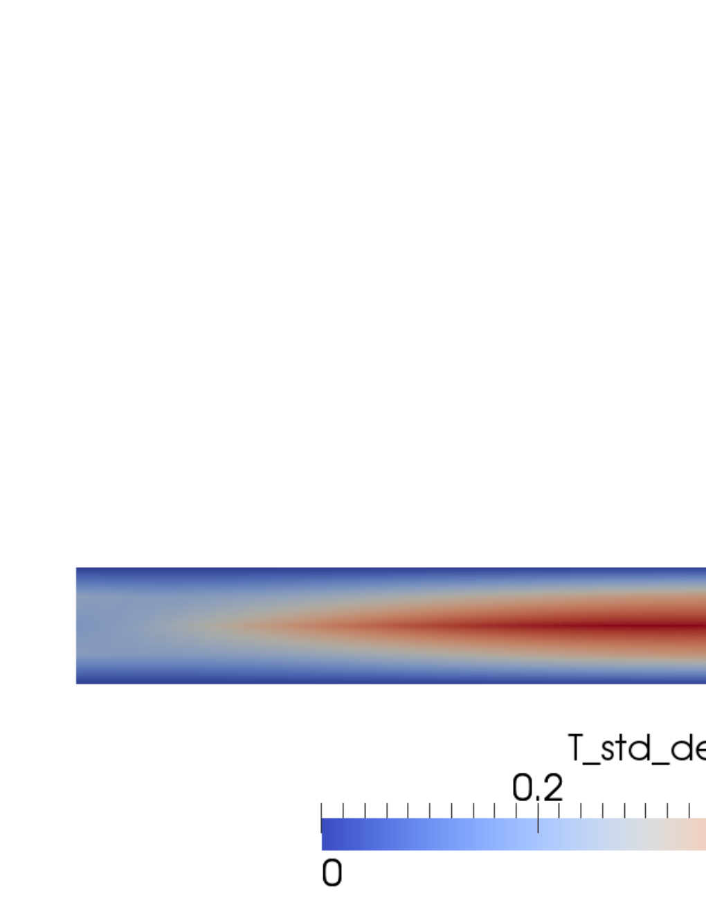
This form of network coupled system is a slight generalization of the system (6), and the techniques presented above can be easily extended to this problem. Given the number of random variables , we apply the nonlinear elimination-based stochastic Galerkin procedure as outlined in Section 2.2 using a total polynomial order . We compute the pseudospectral approximation (see Eq. 22) of the pipe and reactor coupling functions (55) using a tensor-product Gauss-Legendre grid with points for each random variable. Even though uncertainty only appears in the pipe component, its effects must be propagated through the reactor due to the coupling variables and , thus resulting in numerous solves of the reactor problem . All calculations were implemented within the Albany simulation environment leveraging numerous Trilinos [24] packages for assembling and solving the pipe and reactor finite element equations. The finite element solution for each realization of the random variables was computed via a standard Newton method employing a GMRES iterative linear solver preconditioned by an incomplete LU factorization preconditioner. The resulting stochastic Galerkin network equations were assembled and solved using the Stokhos intrusive stochastic Galerkin package [25]. Since the network system after nonlinear elimination is just a system, the cost of solving this system is insignificant compared to the total cost of solving the reactor component at each realization of . Figure 4 shows the resulting mean and standard deviation of the fluid temperature for the uncertain diffusivity field with coefficient of variation of and random variables. The reactor has a temperature source , Reynolds number and mean Rayleigh number .
We then apply the basis reduction and quadrature methods described in Section 3 to the reactor component only. Table 4 compares the resulting total run time for the complete stochastic Galerkin, nonlinear elimination network calculation between both approaches for an increasing number of random variables in the pipe. One can see that for the reduced basis and quadrature approach, the size of the polynomial basis, modified quadrature, and resulting solution time for the reactor component is roughly constant, even though the total number of random variables appearing in the coupled system is increasing.
| Time (sec) | Reduced Time(sec) | |||||||||
|---|---|---|---|---|---|---|---|---|---|---|
| Pipe | Reactor | Total | Pipe | Reactor | Total | |||||
| 2 | 10 | 16 | 10 | 16 | 4 | 62 | 67 | 4 | 53 | 58 |
| 3 | 20 | 64 | 10 | 40 | 17 | 246 | 263 | 17 | 120 | 137 |
| 4 | 35 | 256 | 10 | 41 | 82 | 1052 | 1134 | 73 | 129 | 202 |
| 5 | 56 | 1024 | 10 | 35 | 353 | 4051 | 4405 | 341 | 116 | 458 |
5 Summary & Conclusions
We have presented a method for constructing a polynomial surrogate response surface for the outputs of a network coupled multiphysics system that exploits its structure to increase efficiency. We reduce the full system with a nonlinear elimination method, which results in a smaller system to solve for the coupling terms that depends on the uncertain inputs represented as parameters. We then apply a stochastic Galerkin procedure with a Newton iteration to compute the coefficients of a surrogate response surface that approximates the coupling terms as a polynomial of the input parameters. The residual and Jacobian matrix in the Newton update can be viewed as composite functions: these terms depend on the coupling terms which depend on the uncertain inputs. We take advantage of this composite structure to build a reduced polynomial basis that depend on the coupling terms as intermediate variables. We use this reduced basis to find a modified quadrature rule with relatively few nonzero weights. Each weight equal to zero corresponds to a PDE solve that can be ignored when solving the Newton system. This results in substantial computational savings, which we demonstrated on a simple model of a nuclear reactor.
The method is appropriate when the number of input parameters to the full system is small enough to work with a tensor product quadrature grid. Even though we only evaluate the relatively cheap coupling terms at the full grid to construct the modified quadrature rule, we still have an exponential increase in the number of points in the grid as the dimension of the input space increases; a cheap function evaluated times can still be expensive. This can be alleviated to some extent by standard methods for sensitivity analysis and anisotropic approximation. In principle, sparse grids could also be used in the method by relaxing the non-negativity constraint in the linear program (41), but one must take great care when using sparse grids in conjunction with integration for pseudospectral approximation to maintain discrete orthogonality [26], as well as insuring positive definiteness of the inner products implicit in the QR factorizations (35) and (40). This last difficulty could be alleviated for computing the reduced basis by projecting the monomial matrix (34) onto the original polynomial basis , and thus (35) becomes a standard (unweighted) QR factorization. However one must still choose a sparse grid when defining the modified quadrature rule that has degree of exactness at least for (40). Alternatively, in the spirit of [26], one could incorporate this into a Smolyak sparse grid approach by applying the reduced basis and quadrature techniques to each tensor grid appearing in the Smolyak expansion.
References
- [1] Xiu D, Karniadakis GE. The Wiener-Askey polynomial chaos for stochastic differential equations. SIAM J. Sci. Comput. 2002; 24(2):619–644 (electronic).
- [2] Ghanem RG, Spanos PD. Stochastic finite elements: a spectral approach. Springer-Verlag: New York, 1991.
- [3] LeMaître OP, Knio OM. Spectral Methods for Uncertainty Quantification: With Applications to Computational Fluid Dynamics. Springer, 2010.
- [4] Constantine PG, Phipps ET. A Lanczos method for approximating composite functions. Applied Mathematics and Computation 2012; 218(24):11 751 – 11 762.
- [5] Arnst M, Ghanem R, Phipps E, Red-Horse J. Dimension reduction in stochastic modeling of coupled problems. Int. J. Numer. Meth. Engng 2012; 92(11):940–968.
- [6] Arnst M, Ghanem R, Phipps E, Red-Horse J. Measure transformation and efficient quadrature in reduced-dimensional stochastic modeling of coupled problems. Int. J. Numer. Meth. Engng 2012; 92(12):1044–1080.
- [7] Arnst M, Ghanem R, Phipps E, Red-Horse J. Reduced chaos expansions with random coefficients in reduced-dimensional stochastic modeling of coupled problems. ArXiv e-prints 2012; 1207.0910.
- [8] Porsching T. Jacobi and gauss–seidel methods for nonlinear network problems. SIAM Journal on Numerical Analysis 1969; 6(3):437–449.
- [9] Quarteroni A, Valli A. Domain Decomposition Methods for Partial Differential Equations. Oxford University Press: UK, 2005.
- [10] Glowinski R, Wheeler MF. Domain decomposition and mixed finite element methods for elliptic problems. First International Symposium on Domain Decomposition Methods for Partial Differential Equations, Glowinski R, Golub GH, Meurant GA, Periaux J (eds.), SIAM, 1988; 144–172. Philadelphia.
- [11] Bramble JH, Pasciak JE, Schatz AH. The construction of preconditioners for elliptic problems by substructuring. i. Math. Comput. 1986; 47(175):103–134.
- [12] Bjorstad PE, Widlund OB. Iterative methods for the solution of elliptic problems on regions partitioned into substructures. SIAM J. Numer. Anal. 1986; 23(6):1097–1120.
- [13] Yotov I. A multilevel Newton–Krylov interface solver for multiphysics couplings of flow in porous media. Numer. Linear Algebra Appl 2001; 8(8):551–570.
- [14] Le Maitre OP, Knio OM. Spectral methods for uncertainty quantification With Applications to Computational Fluid Dynamics. Scientific Computation, Springer: New York, 2010.
- [15] Åke Björck. Numerical methods for least squares problems. SIAM, 1996.
- [16] Golub GH, Van Loan CF. Matrix Computations. The Johns Hopkins University Press, 1996.
- [17] Luenberger DG, Ye Y. Linear and Nonlinear Programming. Springer, 2008.
- [18] Gurobi Optimization I. Gurobi optimizer reference manual 2012. URL http://www.gurobi.com.
- [19] Forrest J, de la Nuez D, Lougee-Heimer R. COIN-OR Linear Program Solver. http://www.coin-or.org/Clp/index.html 2012.
- [20] Chae D, Kim SK, Nam HS. Local existence and blow-up criterion of Hölder continuous solutions of the Boussinesq equations. Nagoya Math. J. 1999; 155:55–80.
- [21] Chae D, Imanuvilov OY. Generic solvability of the axisymmetric 3-d euler equations and the 2-d boussinesq equations. J. Diff. Eq. 1999; 156(1):1 – 17.
- [22] Shadid J, Salinger A, Pawlowski R, Lin P, Hennigan G, Tuminaro R, Lehoucq R. Large-scale stabilized FE computational analysis of nonlinear steady-state transport/reaction systems☆. Computer Methods in Applied Mechanics and Engineering Feb 2006; 195(13-16):1846–1871.
- [23] Smith BF, Bjorstad P, Gropp W. Domain Decomposition. Cambridge University Press: UK, 1996.
- [24] Heroux M, Bartlett R, Howle V, Hoekstra R, Hu J, Kolda T, Lehoucq R, Long K, Pawlowski R, Phipps E, et al.. An overview of the Trilinos package. ACM Trans. Math. Softw. 2005; 31(3). http://trilinos.sandia.gov/.
- [25] Phipps ET. Stokhos Stochastic Galerkin Uncertainty Quantification Methods. http://trilinos.sandia.gov/packages/stokhos/ 2011.
- [26] Constantine PG, Eldred MS, Phipps ET. Sparse pseudospectral approximation method. Computer Methods in Applied Mechanics and Engineering 2012; 229-232(0):1–12, 10.1016/j.cma.2012.03.019.