Three-Dimensional Mapped-Grid Finite Volume Modeling of Poroelastic-Fluid Wave Propagation¹¹ 1 Much of this work comes from Section 2.2 and Chapters 8 and 9 of [30]. This is the first widely-distributed version.

Grady I. Lemoine²² 2 Department of Applied Mathematics, University of Washington, Seattle, WA 98195 (gl@uw.edu). Supported in part by NIH grant 5R01AR53652-2 and NSF grants DMS-0914942 and DMS-1216732.

Abstract

This paper extends the author’s previous two-dimensional work with Ou and LeVeque to high-resolution finite volume modeling of systems of fluids and poroelastic media in three dimensions, using logically rectangular mapped grids. A method is described for calculating consistent cell face areas and normal vectors for a finite volume method on a general non-rectilinear hexahedral grid. A novel limiting algorithm is also developed to cope with difficulties encountered in implementing high-resolution finite volume methods for anisotropic media on non-rectilinear grids; the new limiting approach is compatible with any limiter function, and typically reduces solution error even in situations where it is not necessary for correct functioning of the numerical method. Dimensional splitting is used to reduce the computational cost of the solution. The code implementing the three-dimensional algorithms is verified against known plane wave solutions, with particular attention to the performance of the new limiter algorithm in comparison to the classical one. An acoustic wave in brine striking an uneven bed of orthotropic layered sandstone is also simulated in order to demonstrate the capabilities of the simulation code.

keywords

poroelastic, wave propagation, finite-volume, high-resolution, operator splitting, dimensional splitting, mapped grid, interface condition, wave limiter, shear wave

AMS

65M08, 74S10, 74F10, 74J10, 74L05, 74L15, 86-08

1 Introduction

Biot poroelasticity theory is a homogenization technique for modeling the mechanics of a fluid-saturated porous solid. It was developed in the period from the 1930s to the 1960s for problems in soil and rock mechanics [5, 6, 7], but has also found use in in vivo bone [15, 16, 22] and underwater acoustics [11, 23, 24].

In Biot theory, the solid part of the medium (termed the matrix or skeleton) is modeled using linear elasticity, while the fluid is treated using compressible linearized fluid dynamics; Darcy’s law is used to model the aggregate motion of the fluid through the matrix. The interaction of the fluid and solid gives rise to three different types of waves: fast P waves, which are similar to the P waves of elastodynamics; shear waves similar to elastodynamic S waves; and slow P waves, which produce behavior not found in simpler types of media. The interaction of the fluid with the solid part of the medium is important to the behavior of these waves — for the fast P and shear waves, there is little motion of the fluid with respect to the solid, but the slow P waves show relatively large amounts of fluid motion. The viscosity of the pore fluid thus causes light damping and dispersion of the first two wave types, but strong slow P wave damping and a substantial variation of slow P phase velocity with frequency. Carcione provides an excellent treatment of poroelasticity theory in Chapter 7 of his book [12].

A variety of methods have been used to model poroelasticity numerically, including finite difference and pseudospectral [14, 17, 21, 35], finite element [10, 38], boundary element [3], spectral element [19, 36], discontinuous Galerkin [18], and finite volume [32, 37] methods. Semi-analytical methods have been used as well, both in forward problems for their own sake [20] and as the forward solution component of an inversion scheme [8, 9].

Three-dimensional poroelasticity simulation has become somewhat common in recent years due to the increasingly powerful computers available. Recent works on three-dimensional computational poroelasticity on regular grids include those of Naumovich [37], who used a staggered-grid finite volume method on regular, rectilinear grids for isotropic media, and Aldridge et al. [1], who used a staggered-grid finite difference approach. Three-dimensional work capable of using irregular grids includes that of de la Puente et al. [18], who employed a discontinuous Galerkin method on triangular and tetrahedral meshes, and the spectral element work of Morency and Tromp [36].

This paper extends the previous work of Lemoine, Ou, and LeVeque [31, 32] to systems of orthotropic poroelastic and fluid media in three dimensions, modeled using logically rectangular mapped grids. Section 2 develops a first-order linear system of PDEs modeling low-frequency Biot poroelasticity theory, and repeats the interface conditions derived in [31] for convenient reference. Following this, section 3 extends the numerical methods of the previous papers to the three-dimensional system. While most of the extension process is straightforward, some problems occur in 3D that have no counterpart in 2D; section 3.1 discusses a complication that arises when implementing a finite volume method on a non-rectilinear grid of hexahedral cells, while section 3.3 formulates a new wave strength ratio for wave limiting in order to circumvent problems with consistent shear wave identification for mapped grids on orthotropic media. The simulation code implementing these numerical methods is then verified against known plane wave solutions in Section 4, with special attention paid to the behavior of the new limiter algorithm, and results are shown for a poroelastic/fluid demonstration problem showing the ability of the code to model complex systems on mapped grids.

2 Governing equations in three dimensions

2.1 Stress rate-velocity relations

Equations (7.131) and (7.133) of Carcione [12] give the stress-strain relation for an anisotropic poroelastic material in an orthogonal set of axes labeled 1, 2, and 3. Using the summation convention for repeated indices, these equations are

p=M(\zeta-\alpha_{I}e_{I}),\quad\tau_{I}=c_{IJ}^{u}e_{J}-M\alpha_{I}\zeta.

(1)

The quantities in this system are defined as follows:

•

$p$ is the fluid pressure
•

$\zeta$ is the variation of fluid content, $\zeta=-\divg(\phi(\mathbf{u}_{f}-\mathbf{u}_{m}))$
•

$\phi$ is the porosity of the material
•

$\mathbf{u}_{f}$ and $\mathbf{u}_{m}$ are the displacements of the fluid and solid, respectively, from their stress-free configurations
•

$e_{I}$ is the $I$ ’th component of engineering strain, $e=\left(\begin{smallmatrix}\epsilon_{11}&\epsilon_{22}&\epsilon_{33}&\gamma_{23}&\gamma_{13}&\gamma_{12}\end{smallmatrix}\right)^{T}$ . Note that the engineering strains $\gamma_{ij}$ are twice the tensor strains $\epsilon_{ij}$ , $i\neq j$ .
•

$\tau_{I}$ is the $I$ ’th component of the total stress in the material, taken in the same order as the strain
•

$c_{IJ}^{u}=c_{IJ}+\alpha_{I}\alpha_{J}M$ is the undrained elastic stiffness tensor of the matrix
•

$c_{IJ}$ is the drained elastic stiffness tensor of the matrix
•

$\alpha_{I}$ is the $I$ ’th effective stress coefficient, given by $\alpha_{I}=1-\frac{1}{3K_{s}}\sum_{J=1}^{3}c_{IJ}$
•

$K_{s}$ is the bulk modulus of the matrix material
•

$M$ is a parameter related to the bulk compressibility of the medium,

$M=K_{s}\left(\left(1-\frac{K^{*}}{K_{s}}\right)-\phi\left(1-\frac{K_{s}}{K_{f}}\right)\right)^{-1}$ (2)
•

$K_{f}$ is the bulk modulus of the fluid
•

$K^{*}$ is another bulk stiffness coefficient, $K^{*}=\frac{1}{9}\sum_{I=1}^{3}\sum_{J=1}^{3}c_{IJ}$

To begin building a first-order velocity-stress system, note the following relations between velocities and strain rates (presuming space and time derivatives can be interchanged):

	$\displaystyle\begin{aligned} \partial_{t}e_{1}&=v_{1,1},\quad&\partial_{t}e_{2}&=v_{2,2},\quad&\partial_{t}e_{3}&=v_{3,3},\\ \partial_{t}e_{4}&=v_{2,3}+v_{3,2},\quad&\partial_{t}e_{5}&=v_{1,3}+v_{3,1},\quad&\partial_{t}e_{6}&=v_{1,2}+v_{2,1},\\ \end{aligned}$		(3)
	$\displaystyle\partial_{t}\zeta=-q_{1,1}-q_{2,2}-q_{3,3}.$		(4)

Here $\mathbf{v}$ is the velocity of the matrix relative to an inertial frame, and $\mathbf{q}$ is the flow rate of the fluid relative to the matrix (the porosity $\phi$ times the aggregate velocity of the fluid relative to the matrix). Subscript indices before a comma represent components, while those after a comma represent differentiation. Differentiating (1) with respect to time, and defining the vectors of stresses and velocities as $\mbox{$\mathbf{Q}$}_{s}=\left(\begin{smallmatrix}\tau_{11}&\tau_{22}&\tau_{33}&\tau_{23}&\tau_{13}&\tau_{12}&p\end{smallmatrix}\right)^{T}$ and $\mbox{$\mathbf{Q}$}_{v}=\left(\begin{smallmatrix}v_{1}&v_{2}&v_{3}&q_{1}&q_{2}&q_{3}\end{smallmatrix}\right)^{T}$ , results in a system relating $\partial_{t}\mbox{$\mathbf{Q}$}_{s}$ to the gradients of the velocities:

\partial_{t}\mbox{$\mathbf{Q}$}_{s}+\mbox{$\mathbf{A}$}_{sv}\mbox{$\mathbf{Q}$}_{v,1}+\mbox{$\mathbf{B}$}_{sv}\mbox{$\mathbf{Q}$}_{v,2}+\mathbf{C}_{sv}\mbox{$\mathbf{Q}$}_{v,3}=0.

(5)

Rather than give the matrices $\mbox{$\mathbf{A}$}_{sv}$ , $\mbox{$\mathbf{B}$}_{sv}$ , and $\mathbf{C}_{sv}$ individually, it is more convenient to write the matrix $\breve{\mbox{$\mathbf{A}$}}_{sv}=n_{1}\mbox{$\mathbf{A}$}_{sv}+n_{2}\mbox{$\mathbf{B}$}_{sv}+n_{3}\mathbf{C}_{sv}$ that is the coefficient of the directional derivative of $\mbox{$\mathbf{Q}$}_{v}$ in the $(n_{1},n_{2},n_{3})$ direction. If the medium is orthotropic, and the 1-2-3 axes are its principal axes, then

\breve{\mbox{$\mathbf{A}$}}_{sv}=-\begin{pmatrix}n_{1}c_{11}^{u}&n_{2}c_{12}^{u}&n_{3}c_{13}^{u}&n_{1}\alpha_{1}M&n_{2}\alpha_{1}M&n_{3}\alpha_{1}M\\ n_{1}c_{12}^{u}&n_{2}c_{22}^{u}&n_{3}c_{23}^{u}&n_{1}\alpha_{2}M&n_{2}\alpha_{2}M&n_{3}\alpha_{2}M\\ n_{1}c_{13}^{u}&n_{2}c_{23}^{u}&n_{3}c_{33}^{u}&n_{1}\alpha_{3}M&n_{2}\alpha_{3}M&n_{3}\alpha_{3}M\\ 0&n_{3}c_{44}&n_{2}c_{44}&0&0&0\\ n_{3}c_{55}&0&n_{1}c_{55}&0&0&0\\ n_{2}c_{66}&n_{1}c_{66}&0&0&0&0\\ -n_{1}M\alpha_{1}&-n_{2}M\alpha_{2}&-n_{3}M\alpha_{3}&-n_{1}M&-n_{2}M&-n_{3}M\end{pmatrix}.

(6)

2.2 Equations of motion

System (5) does not yet provide a closed set of equations that can be used to describe the dynamics of the poroelastic medium. Equations of motion are still required that relate accelerations to gradients of stress. Equations (7.255) and (7.256) of [12] provide the key. If the medium is orthotropic and the 1-2-3 axes are its principal axes, they relate accelerations to stress gradients:

	$\displaystyle\tau_{ij,j}$	$\displaystyle=\rho\partial_{t}^{2}u_{mi}+\rho_{f}\partial_{t}^{2}w_{i}$		(7)
	$\displaystyle-p_{,i}$	$\displaystyle=\rho_{f}\partial_{t}^{2}u_{mi}+m_{i}\partial_{t}^{2}w_{i}+\frac{\eta}{\kappa_{i}}\partial_{t}w_{i}.$		(7)

Here $i$ ranges from 1 to 3; there is a sum over $j$ in the first equation, but no sum over $i$ in the second. The new variables in these equations are as follows:

•

$\rho$ is the bulk density of the medium, $\rho=(1-\phi)\rho_{s}+\phi\rho_{f}$
•

$\rho_{s}$ is the density of the matrix material
•

$\rho_{f}$ is the density of the fluid
•

$\mathbf{w}$ is the displacement of the fluid relative to the matrix, scaled by the porosity. The rate of change of $\mathbf{w}$ is $\partial_{t}\mathbf{w}=\mathbf{q}$ .
•

$m_{i}$ is the fluid inertia along axis $i$ , $m_{i}=\rho_{f}T_{i}/\phi$
•

$T_{i}$ is the tortuosity of the matrix along axis $i$ , defined as the factor by which the kinetic energy of the fluid must be higher than its density would indicate for straight-line motion, in order to have a given bulk velocity along that axis

For each $i$ , (7) is a system of two equations in two unknowns. Noting that $\partial_{t}u_{mi}=v_{i}$ , this system becomes

	$\displaystyle\rho\partial_{t}v_{i}+\rho_{f}\partial_{t}q_{i}$	$\displaystyle=\tau_{ij,j}$		(8)
	$\displaystyle\rho_{f}\partial_{t}v_{i}+m_{i}\partial_{t}q_{i}$	$\displaystyle=-p_{,i}-\frac{\eta}{\kappa_{i}}q_{i}.$		(8)

Solving with Cramer’s Rule results in

	$\displaystyle\partial_{t}v_{i}$	$\displaystyle=\frac{m_{i}}{\Delta_{i}}\tau_{ij,j}+\frac{\rho_{f}}{\Delta_{i}}p_{,i}+\frac{\rho_{f}\eta}{\Delta_{i}\kappa_{i}}q_{i}$		(9)
	$\displaystyle\partial_{t}q_{i}$	$\displaystyle=-\frac{\rho_{f}}{\Delta_{i}}\tau_{ij,j}-\frac{\rho}{\Delta_{i}}p_{,i}-\frac{\rho\eta}{\Delta_{i}\kappa_{i}}q_{i},$		(9)

where $\Delta_{i}:=\rho m_{i}-\rho_{f}^{2}$ .

It is now possible to write a linear system relating the rates of change of the velocities to the gradients of stress, of the form

\partial_{t}\mbox{$\mathbf{Q}$}_{v}+\mbox{$\mathbf{A}$}_{vs}\mbox{$\mathbf{Q}$}_{s,1}+\mbox{$\mathbf{B}$}_{vs}\mbox{$\mathbf{Q}$}_{s,2}+\mathbf{C}_{vs}\mbox{$\mathbf{Q}$}_{s,3}=\mbox{$\mathbf{D}$}_{v}\mbox{$\mathbf{Q}$}_{v}.

(10)

Again, it is more convenient to provide $\breve{\mbox{$\mathbf{A}$}}_{vs}=n_{1}\mbox{$\mathbf{A}$}_{vs}+n_{2}\mbox{$\mathbf{B}$}_{vs}+n_{3}\mathbf{C}_{vs}$ , rather than the individual matrices of (10):

\breve{\mbox{$\mathbf{A}$}}_{vs}=-\begin{pmatrix}n_{1}\frac{m_{1}}{\Delta_{1}}&0&0&0&n_{3}\frac{m_{1}}{\Delta_{1}}&n_{2}\frac{m_{1}}{\Delta_{1}}&n_{1}\frac{\rho_{f}}{\Delta_{1}}\\ 0&n_{2}\frac{m_{2}}{\Delta_{2}}&0&n_{3}\frac{m_{2}}{\Delta_{2}}&0&n_{1}\frac{m_{2}}{\Delta_{2}}&n_{2}\frac{\rho_{f}}{\Delta_{2}}\\ 0&0&n_{3}\frac{m_{3}}{\Delta_{3}}&n_{2}\frac{m_{3}}{\Delta_{3}}&n_{1}\frac{m_{3}}{\Delta_{3}}&0&n_{3}\frac{\rho_{f}}{\Delta_{3}}\\ -n_{1}\frac{\rho_{f}}{\Delta_{1}}&0&0&0&-n_{3}\frac{\rho_{f}}{\Delta_{1}}&-n_{2}\frac{\rho_{f}}{\Delta_{1}}&-n_{1}\frac{\rho}{\Delta_{1}}\\ 0&-n_{2}\frac{\rho_{f}}{\Delta_{2}}&0&-n_{3}\frac{\rho_{f}}{\Delta_{2}}&0&-n_{1}\frac{\rho_{f}}{\Delta_{2}}&-n_{2}\frac{\rho}{\Delta_{2}}\\ 0&0&-n_{3}\frac{\rho_{f}}{\Delta_{3}}&-n_{2}\frac{\rho_{f}}{\Delta_{3}}&-n_{1}\frac{\rho_{f}}{\Delta_{3}}&0&-n_{3}\frac{\rho}{\Delta_{3}}\end{pmatrix}.

(11)

The matrix $\mbox{$\mathbf{D}$}_{v}$ models the viscous dissipation, and is given by

\mbox{$\mathbf{D}$}_{v}=\begin{pmatrix}0&0&0&\frac{\rho_{f}\eta}{\Delta_{1}\kappa_{1}}&0&0\\ 0&0&0&0&\frac{\rho_{f}\eta}{\Delta_{2}\kappa_{2}}&0\\ 0&0&0&0&0&\frac{\rho_{f}\eta}{\Delta_{3}\kappa_{3}}\\ 0&0&0&-\frac{\rho\eta}{\Delta_{1}\kappa_{1}}&0&0\\ 0&0&0&0&-\frac{\rho\eta}{\Delta_{2}\kappa_{2}}&0\\ 0&0&0&0&0&-\frac{\rho\eta}{\Delta_{3}\kappa_{3}}\end{pmatrix}.

(12)

2.3 First-order velocity-stress system

Combining (5) and (10), and letting the full 13-element state vector be $\mbox{$\mathbf{Q}$}=\left(\begin{smallmatrix}\mbox{$\mathbf{Q}$}_{s}^{T}&\mbox{$\mathbf{Q}$}_{v}^{T}\end{smallmatrix}\right)^{T}$ , the first-order stress-velocity system describing three-dimensional poroelasticity is

\partial_{t}\mbox{$\mathbf{Q}$}+\mbox{$\mathbf{A}$}\mbox{$\mathbf{Q}$}_{,1}+\mbox{$\mathbf{B}$}\mbox{$\mathbf{Q}$}_{,2}+\mathbf{C}\mbox{$\mathbf{Q}$}_{,3}=\mbox{$\mathbf{D}$}\mbox{$\mathbf{Q}$},

(13)

where

	$\displaystyle\mbox{$\mathbf{A}$}$	$\displaystyle=\begin{pmatrix}0_{7\times 7}&\mbox{$\mathbf{A}$}_{sv}\\ \mbox{$\mathbf{A}$}_{vs}&0_{6\times 6}\end{pmatrix},$	$\displaystyle\mbox{$\mathbf{B}$}$	$\displaystyle=\begin{pmatrix}0_{7\times 7}&\mbox{$\mathbf{B}$}_{sv}\\ \mbox{$\mathbf{B}$}_{vs}&0_{6\times 6}\end{pmatrix},$		(14)
	$\displaystyle\mathbf{C}$	$\displaystyle=\begin{pmatrix}0_{7\times 7}&\mathbf{C}_{sv}\\ \mathbf{C}_{vs}&0_{6\times 6}\end{pmatrix},$	$\displaystyle\mbox{$\mathbf{D}$}$	$\displaystyle=\begin{pmatrix}0_{7\times 7}&0_{6\times 7}\\ 0_{7\times 6}&\mbox{$\mathbf{D}$}_{v}\end{pmatrix}.$		(14)

The reader should note that, as in [32], this system describes low-frequency Biot poroelasticity theory — that is, it is valid only for angular frequencies below the critical value $\omega_{c}:=\min_{i}\frac{\eta\phi}{\rho_{f}T_{i}\kappa_{i}}$ .

2.4 Energy density

Since the constitutive relation of the poroelastic medium is linear, the strain energy $V$ is just half the sum of the products of the stresses with their corresponding strains,

\mathcal{V}=\frac{1}{2}\left(\sum_{I=1}^{6}\tau_{I}e_{I}+p\zeta\right)=\frac{1}{2}\left(\mbox{\boldmath$\tau$}^{T}\mathbf{e}+p\zeta\right).

(15)

Using equation (7.132) from [12], $\tau_{I}=c_{IJ}e_{J}-\alpha_{I}p$ , we can write $c_{IJ}e_{J}=\tau_{I}+\alpha_{I}p$ . (Note that in the principal axes of an orthotropic material, $\alpha_{I}=0$ for $I>3$ — there is no equivalent shear stress in the principal axes associated with the fluid pressure.) Letting $\mathbf{S}$ be the compliance matrix of the drained skeleton — the inverse of the matrix formed by the drained elastic parameters $c_{IJ}$ — in matrix notation we have

\mathbf{e}=\mathbf{S}(\mbox{\boldmath$\tau$}+p\mbox{\boldmath$\alpha$}).

(16)

Here $\tau$ and $\mathbf{e}$ are arranged as $6\times 1$ column vectors, not as symmetric $3\times 3$ matrices.

To get the variation of fluid content $\zeta$ , let us return to equation (7.131) of [12], $p=M(\zeta-\alpha_{I}e_{I})$ . In matrix notation, this is $p=M(\zeta-\mbox{\boldmath$\alpha$}^{T}\mathbf{e})=M(\zeta-\mbox{\boldmath$\alpha$}^{T}\mathbf{S}\mbox{\boldmath$\tau$}-p\mbox{\boldmath$\alpha$}^{T}\mathbf{S}\mbox{\boldmath$\alpha$})$ . Solving for $\zeta$ in terms of the stress variables gives

\zeta=\left(\tfrac{1}{M}+\mbox{\boldmath$\alpha$}^{T}\mathbf{S}\mbox{\boldmath$\alpha$}\right)p+\mbox{\boldmath$\alpha$}^{T}\mathbf{S}\mbox{\boldmath$\tau$}.

(17)

Substituting (16) and (17) into (15), and using the symmetry of $\mathbf{S}$ , we get

\mathcal{V}=\tfrac{1}{2}\left(\mbox{\boldmath$\tau$}^{T}\mathbf{S}\mbox{\boldmath$\tau$}+2p\mbox{\boldmath$\alpha$}^{T}\mathbf{S}\mbox{\boldmath$\tau$}+p^{2}\left(\tfrac{1}{M}+\mbox{\boldmath$\alpha$}^{T}\mathbf{S}\mbox{\boldmath$\alpha$}\right)\right).

(18)

In matrix form this is

\mathcal{V}=\tfrac{1}{2}\mbox{$\mathbf{Q}$}_{s}^{T}\mbox{$\mathbf{E}$}_{s}\mbox{$\mathbf{Q}$}_{s},\quad\mbox{$\mathbf{E}$}_{s}:=\begin{pmatrix}\mathbf{S}&\mathbf{S}\mbox{\boldmath$\alpha$}\\ \mbox{\boldmath$\alpha$}^{T}\mathbf{S}&\tfrac{1}{M}+\mbox{\boldmath$\alpha$}^{T}\mathbf{S}\mbox{\boldmath$\alpha$}\end{pmatrix}.

(19)

Meanwhile, the derivation of kinetic energy from the two-dimensional case in [32] carries over directly to three dimensions, and the kinetic energy is

\mathcal{T}=\tfrac{1}{2}\mbox{$\mathbf{Q}$}_{v}^{T}\mbox{$\mathbf{E}$}_{v}\mbox{$\mathbf{Q}$}_{v},

(20)

where the matrix $\mbox{$\mathbf{E}$}_{v}$ is

\mbox{$\mathbf{E}$}_{v}=\begin{pmatrix}\rho\mathbf{I}_{3\times 3}&\rho_{f}\mathbf{I}_{3\times 3}\\ \rho_{f}\mathbf{I}_{3\times 3}&\mathop{\operator@font diag}\nolimits(m_{1},m_{2},m_{3})\end{pmatrix}.

(21)

Combining (19) and (20) gives the total energy per unit volume in terms of the state vector $\mathbf{Q}$ as

\mathcal{E}=\mathcal{T}+\mathcal{V}=\tfrac{1}{2}\mbox{$\mathbf{Q}$}^{T}\mbox{$\mathbf{E}$}\mbox{$\mathbf{Q}$},\quad\mbox{$\mathbf{E}$}:=\begin{pmatrix}\mbox{$\mathbf{E}$}_{s}&0_{7\times 6}\\ 0_{6\times 7}&\mbox{$\mathbf{E}$}_{v}\end{pmatrix}.

(22)

We may expect $\mathbf{E}$ to be positive-definite on physical grounds — if it were not, it would be possible to deform the medium, change its fluid content, or set it in motion without doing work.

2.5 Symmetrization

In terms of the block structure of the system, $\mbox{$\mathbf{E}$}\breve{\mbox{$\mathbf{A}$}}$ is symmetric if and only if $\mbox{$\mathbf{E}$}_{s}\breve{\mbox{$\mathbf{A}$}}_{sv}=(\mbox{$\mathbf{E}$}_{v}\breve{\mbox{$\mathbf{A}$}}_{vs})^{T}$ . After substantial algebra, it can in fact be shown that

\mbox{$\mathbf{E}$}_{s}\breve{\mbox{$\mathbf{A}$}}_{sv}=(\mbox{$\mathbf{E}$}_{v}\breve{\mbox{$\mathbf{A}$}}_{vs})^{T}=-\begin{pmatrix}n_{1}&0&0&0&0&0\\ 0&n_{2}&0&0&0&0\\ 0&0&n_{3}&0&0&0\\ 0&n_{3}&n_{2}&0&0&0\\ n_{3}&0&n_{1}&0&0&0\\ n_{2}&n_{1}&0&0&0&0\\ 0&0&0&-n_{1}&-n_{2}&-n_{3}\end{pmatrix}.

(23)

Thus $\mathbf{E}$ does indeed symmetrize the system.

Since $\mathbf{E}$ symmetrizes the system, we immediately know that the governing equations of three-dimensional poroelasticity are hyperbolic by the argument of Section 2.7 of [32]. An energy norm and energy inner product can also be defined in exactly the same fashion as in that work. Furthermore, we can easily see that $\mathbf{E}$ $\mathbf{D}$ is a symmetric negative-semidefinite matrix in three dimensions as well, since

\mbox{$\mathbf{E}$}\mbox{$\mathbf{D}$}=\begin{pmatrix}0_{10\times 10}&0_{10\times 3}\\ 0_{3\times 10}&-\mathop{\operator@font diag}\nolimits\left(\eta/\kappa_{1},\eta/\kappa_{2},\eta/\kappa_{3}\right)\end{pmatrix}.

(24)

By the arguments of Section 2.8 of [32], almost all of the conditions are satisfied for the energy density $\mathcal{E}$ to be a strictly convex entropy function in the sense of Chen, Levermore, and Liu [13]. There is one final condition, involving the operator $\mathbf{\Pi}$ that maps from the full to the reduced system; following Section 3.3 of [32], in three dimensions the matrix $\mathbf{\Pi}$ that maps from the full poroelastic state vector $\mathbf{Q}$ to the vector of conserved quantities of the dissipation part of the system $\mathbf{u}$ is

\mathbf{\Pi}:=\begin{pmatrix}\mathbf{I}_{7\times 7}&0_{7\times 6}\\ 0_{3\times 7}&\mathbf{\Pi}_{v}\end{pmatrix},\quad\mathbf{\Pi}_{v}:=\begin{pmatrix}1&0&0&\rho_{f}/\rho&0&0\\ 0&1&0&0&\rho_{f}/\rho&0\\ 0&0&1&0&0&\rho_{f}/\rho\end{pmatrix}

(25)

As in two dimensions, the fact that $\mathbf{u}$ is conserved under the action of the dissipation can be seen immediately because $\mathbf{\Pi}\mbox{$\mathbf{D}$}=0$ . The matrix $\mathbf{G}$ that from any $\mathbf{u}$ gives the unique equilibrium $\mbox{$\mathbf{Q}$}_{\text{eq}}$ satisfying both $\mbox{$\mathbf{D}$}\mbox{$\mathbf{Q}$}_{\text{eq}}=0$ and $\mathbf{\Pi}\mbox{$\mathbf{Q}$}_{\text{eq}}=\mathbf{u}$ is

\mbox{$\mathbf{G}$}:=\begin{pmatrix}\mathbf{I}_{10\times 10}\\ 0_{3\times 10}\end{pmatrix}.

(26)

From these two matrices, the reduced system can be formed:

\partial_{t}\mathbf{u}+\mathbf{\Pi}\mbox{$\mathbf{A}$}\mbox{$\mathbf{G}$}\mathbf{u}_{,1}+\mathbf{\Pi}\mbox{$\mathbf{B}$}\mbox{$\mathbf{G}$}\mathbf{u}_{,2}+\mathbf{\Pi}\mathbf{C}\mbox{$\mathbf{G}$}\mathbf{u}_{,3}=0.

(27)

The matrix $\mathbf{\Pi}$ allows us to see that the statements $\mbox{$\mathbf{D}$}\mbox{$\mathbf{Q}$}=0$ and $\mathcal{E}^{\prime}(\mbox{$\mathbf{Q}$})^{T}\mbox{$\mathbf{D}$}\mbox{$\mathbf{Q}$}=\mbox{$\mathbf{Q}$}^{T}\mbox{$\mathbf{E}$}\mbox{$\mathbf{D}$}\mbox{$\mathbf{Q}$}=0$ are equivalent to $\mbox{$\mathbf{Q}$}^{T}\mbox{$\mathbf{E}$}=\mathbf{v}^{T}\mathbf{\Pi}$ for some $\mathbf{v}\in\mathbb{R}^{10}$ . As in [32], if $\mbox{$\mathbf{Q}$}^{T}\mathbf{E}=\mathbf{v}^{T}\mathbf{\Pi}$ , we immediately have $\mbox{$\mathbf{Q}$}^{T}\mathbf{E}\mbox{$\mathbf{D}$}\mbox{$\mathbf{Q}$}=\mathbf{v}^{T}\mathbf{\Pi}\mbox{$\mathbf{D}$}\mbox{$\mathbf{Q}$}=0$ since $\mathbf{\Pi}\mbox{$\mathbf{D}$}=0$ . Conversely, if $\mbox{$\mathbf{D}$}\mbox{$\mathbf{Q}$}=0$ , the form of $\mathbf{D}$ also immediately gives $q_{x}=q_{y}=q_{z}=0$ . Thus in this case the last six components of $\mbox{$\mathbf{Q}$}^{T}\mbox{$\mathbf{E}$}$ are $(\mbox{$\mathbf{Q}$}^{T}\mathbf{E})_{8}=\rho v_{x}$ , $(\mbox{$\mathbf{Q}$}^{T}\mathbf{E})_{9}=\rho v_{y}$ , $(\mbox{$\mathbf{Q}$}^{T}\mathbf{E})_{10}=\rho v_{z}$ , $(\mbox{$\mathbf{Q}$}^{T}\mathbf{E})_{11}=\rho_{f}v_{x}$ , $(\mbox{$\mathbf{Q}$}^{T}\mathbf{E})_{12}=\rho_{f}v_{y}$ , and $(\mbox{$\mathbf{Q}$}^{T}\mathbf{E})_{13}=\rho_{f}v_{z}$ . This implies that if $\mbox{$\mathbf{D}$}\mbox{$\mathbf{Q}$}=0$ , $\mbox{$\mathbf{Q}$}^{T}\mbox{$\mathbf{E}$}=\mathbf{v}^{T}\mathbf{\Pi}$ , with $\mathbf{v}$ given by

\mathbf{v}^{T}=\begin{pmatrix}\mbox{$\mathbf{Q}$}_{s}^{T}\mbox{$\mathbf{E}$}_{s}&\rho v_{x}&\rho v_{y}&\rho v_{z}\end{pmatrix}.

(28)

Here the stress parts of $\mathbf{Q}$ and $\mathbf{E}$ have been separated out for convenience.

As in two-dimensional poroelasticity, this condition implies that the reduced system (27) is hyperbolic, and satisfies a nonstrict subcharacteristic condition. Equality can again be realized in the subcharacteristic condition — the example of this found in Section 3.3 of [32] carries over to three dimensions — but the argument from two dimensions that this is harmless to the numerical solution also carries over to three dimensions. In addition, the matrix $\mathbf{\Pi}\breve{\mbox{$\mathbf{A}$}}\mbox{$\mathbf{G}$}$ again takes the form of orthotropic elasticity, with the fluid pressure coming along as an additional variable that does not feed back into the elastic variables. The flux Jacobian of the reduced system is

\mathbf{\Pi}\breve{\mbox{$\mathbf{A}$}}\mbox{$\mathbf{G}$}=\begin{pmatrix}0&0&0&0&0&0&0&-n_{1}c_{11}^{u}&-n_{2}c_{12}^{u}&-n_{3}c_{13}^{u}\\ 0&0&0&0&0&0&0&-n_{1}c_{12}^{u}&-n_{2}c_{22}^{u}&-n_{3}c_{23}^{u}\\ 0&0&0&0&0&0&0&-n_{1}c_{13}^{u}&-n_{2}c_{23}^{u}&-n_{3}c_{33}^{u}\\ 0&0&0&0&0&0&0&0&-n_{3}c_{44}&-n_{2}c_{44}\\ 0&0&0&0&0&0&0&-n_{3}c_{55}&0&-n_{1}c_{55}\\ 0&0&0&0&0&0&0&-n_{2}c_{66}&-n_{1}c_{66}&0\\ 0&0&0&0&0&0&0&n_{1}M\alpha_{1}&n_{2}M\alpha_{2}&n_{3}M\alpha_{3}\\ -\frac{n_{1}}{\rho}&0&0&0&-\frac{n_{3}}{\rho}&-\frac{n_{2}}{\rho}&0&0&0&0\\ 0&-\frac{n_{2}}{\rho}&0&-\frac{n_{3}}{\rho}&0&-\frac{n_{1}}{\rho}&0&0&0&0\\ 0&0&-\frac{n_{3}}{\rho}&-\frac{n_{2}}{\rho}&-\frac{n_{1}}{\rho}&0&0&0&0&0\end{pmatrix}.

(29)

2.6 Linear acoustics

For this work the PDEs of acoustics will be cast in the same form as the poroelastic system (13), with the same state vector; however, in a fluid the variables $\tau$ and $\mathbf{v}$ will be defined to be identically zero, as in [31]. The state variable $p$ will be used for the fluid pressure, and $\mathbf{q}$ for its velocity. The three-dimensional system’s coefficient matrices have the same block form as those for poroelasticity; the blocks are

\displaystyle\breve{\mbox{$\mathbf{A}$}}_{sv}

\displaystyle=\begin{pmatrix}0_{6\times 3}&0_{6\times 3}\\ 0_{1\times 3}&K_{f}\mathbf{n}^{T}\end{pmatrix},

\displaystyle\breve{\mbox{$\mathbf{A}$}}_{vs}

\displaystyle=\begin{pmatrix}0_{3\times 6}&0_{3\times 1}\\ 0_{3\times 6}&\mathbf{n}/\rho_{f}\end{pmatrix}.

(30)

The properties of a fluid are assumed isotropic, so $\breve{\mbox{$\mathbf{A}$}}=n_{x}\mbox{$\mathbf{A}$}+n_{y}\mbox{$\mathbf{B}$}+n_{z}\mathbf{C}$ here is written in terms of a vector $\mathbf{n}=(n_{x},n_{y},n_{z})$ in the global problem coordinates. (When used in linear algebra, $\mathbf{n}$ is taken to be a column vector.) In a fluid, the dissipation matrix $\mathbf{D}$ is identically zero.

Just as with poroelasticity, linear acoustics also possesses an energy density that can be expressed as a quadratic form, $\mathcal{E}=\frac{1}{2}\mbox{$\mathbf{Q}$}^{T}\mbox{$\mathbf{E}$}\mbox{$\mathbf{Q}$}$ . The energy divides neatly into kinetic and potential, giving the same block structure for $\mathbf{E}$ as before, with the blocks for acoustics equal to

\mbox{$\mathbf{E}$}_{s}=\begin{pmatrix}0_{6\times 6}&0_{6\times 1}\\ 0_{1\times 6}&1/K_{f}\end{pmatrix},\quad\mbox{$\mathbf{E}$}_{v}=\begin{pmatrix}0_{3\times 3}&0_{3\times 3}\\ 0_{3\times 3}&\rho_{f}\mathbf{I}_{3\times 3}\end{pmatrix}

(31)

This matrix $\mathbf{E}$ is only positive-semidefinite, not positive-definite as for poroelasticity. Similarly to the two-dimensional case discussed in [31], however, the null space of $\mathbf{E}$ consists only of the variables that are defined to be identically zero in the fluid. This means $\mathbf{E}$ is essentially positive-definite, and can still be used to define an energy inner product and norm for acoustics. Just as for poroelasticity, $\mathbf{E}$ symmetrizes the first-order hyperbolic system for acoustics.

2.7 Interface conditions

The same interface conditions are used here in three dimensions as were used in two dimensions in [31] — and in fact the same vector formulas may be used, since the ones written in Section 2.4 of [31] are equally valid in two or three dimensions.

To reprise, open pores, closed pores, or imperfect hydraulic contact between two poroelastic media may be expressed as the set of conditions

$\displaystyle\mbox{\boldmath$\tau$}_{l}\cdot\mathbf{n}$	$\displaystyle=\mbox{\boldmath$\tau$}_{r}\cdot\mathbf{n}$	(32)
$\displaystyle\mathbf{v}_{l}$	$\displaystyle=\mathbf{v}_{r}$
$\displaystyle\mathbf{q}_{l}\cdot\mathbf{n}$	$\displaystyle=\mathbf{q}_{r}\cdot\mathbf{n}$
$\displaystyle\eta_{d}(p_{l}-p_{r})$	$\displaystyle=Z_{f}(1-\eta_{d})\widehat{\mathbf{q}\cdot\mathbf{n}},$

where the subscripts $l$ and $r$ denote the arbitrarily-chosen left and right sides of the interface, the vector $\mathbf{n}$ is the unit interface normal pointing from the left medium to the right one, $Z_{f}$ is the acoustic impedance of the fluid in the left medium, and $\eta_{d}$ is the interface discharge efficiency, a nondimensional measure of the resistance of the interface to fluid flow. In this formulation, $\eta_{d}=1$ corresponds to fluid flowing across the interface unhindered, while $\eta_{d}=0$ corresponds to a completely impermeable interface, and values of $\eta_{d}$ between 0 and 1 indicate an interface that allows fluid to pass, but only if driven by a pressure difference. The quantity $\widehat{\mathbf{q}\cdot\mathbf{n}}$ is equal to both $\mathbf{q}_{l}\cdot\mathbf{n}$ and $\mathbf{q}_{r}\cdot\mathbf{n}$ . Similar interface conditions between a poroelastic medium and a fluid may be expressed as

$\displaystyle\mathbf{q}_{f}\cdot\mathbf{n}$	$\displaystyle=(\mathbf{v}_{p}+\mathbf{q}_{p})\cdot\mathbf{n}$	(33)
$\displaystyle-p_{f}\mathbf{n}$	$\displaystyle=\mbox{\boldmath$\tau$}_{p}\cdot\mathbf{n}$
$\displaystyle\eta_{d}(p_{p}-p_{f})$	$\displaystyle=Z_{f}(1-\eta_{d})\mathbf{q}_{p}\cdot\mathbf{n},$

where $Z_{f}$ is the impedance of the fluid medium, the subscripts $p$ and $f$ denote the poroelastic and fluid media, and the unit vector $\mathbf{n}$ points from the poroelastic medium into the fluid.

3 Finite volume methods for mapped grids in three dimensions

Despite the increase in the number of spatial dimensions and the expansion of the state vector from 8 to 13 elements, most of the details of the numerical method for three-dimensional poroelasticity and poroelastic-fluid systems on mapped grids are closely analogous to the two-dimensional methods of [32] and [31]. It is primarily the changes between the two-dimensional and three dimensional method that are described here. Section 3.1 describes how mapped grids are used in three dimensions, while in Section 3.2 the Riemann solution process is discussed, including the interface condition matrices used to solve the Riemann problem between a fluid and a poroelastic medium in three dimensions.

There are also some algorithmic details that differ between two dimensions and three. Specifically, the combination of mapped grids and anisotropic materials requires a change to the limiter algorithm in order to cope with potential difficulties in consistently tracking the polarization of the shear waves; this change is discussed and evaluated in two dimensions in Section 3.3. Also, since the transverse Riemann solutions for three-dimensional high-resolution finite volume methods are both computationally expensive and time-consuming to program, dimensional splitting becomes very attractive. While dimensional splitting is by no means a new algorithmic development, Section 3.4 gives a simple overview. Finally, Section 3.5 gives a brief summary of the software frameworks in which these algorithms are implemented.

3.1 Mapped grids in three dimensions

As in [31], the three-dimensional numerical solution procedure uses logically rectangular mapped grids. In three dimensions, though, mapped grid quantities such as interface normals and cell face areas are more difficult to define.

Each cell in the mapped grid is defined by the physical coordinates of its vertices, which are computed by applying the mapping function to the vertices of the cell in the computational domain. Physical coordinates will be denoted by $x$ , $y$ , and $z$ , or the position vector $\mathbf{r}$ , while computational coordinates are $\xi_{1}$ , $\xi_{2}$ , and $\xi_{3}$ . From its vertices, cells are defined by a trilinear mapping. Let $\eta_{1}$ , $\eta_{2}$ , and $\eta_{3}$ be cell-local computational coordinates, defined from the global computational coordinates by

\eta_{i}=\frac{\xi_{i}-\xi_{i0}}{\Delta\xi_{i}},

(34)

where $\xi_{i0}$ is the lowest extent of the cell in global computational coordinate $i$ and $\Delta\xi_{i}$ is the grid spacing in computational coordinate $i$ . In local computational coordinates, the cell is thus the unit cube $[0,1]^{3}$ . From these coordinates, the cell is parameterized in physical coordinates by

\mathbf{r}(\eta_{1},\eta_{2},\eta_{3})=\sum_{i=1}^{2}\sum_{j=1}^{2}\sum_{k=1}^{2}\mathbf{r}_{ijk}N_{i}(\eta_{1})N_{j}(\eta_{2})N_{k}(\eta_{3}),

(35)

where the $\mathbf{r}_{ijk}$ are the vertices, with each subscript denoting the position in the corresponding computational direction (so for example $\mathbf{r}_{112}$ is the $-\xi_{1}$ , $-\xi_{2}$ , $+\xi_{3}$ vertex), and the $N$ functions are $N_{1}(\eta)=1-\eta$ , $N_{2}(\eta)=\eta$ .

Defining the normal vector to a cell face stretched between four essentially arbitrary vertices is not trivial, because the vertices may not be coplanar. A sensible requirement, though, seems to be for the normal $\mathbf{n}$ and area $A$ of a face to satisfy

\mathbf{n}A=\int_{\text{face}}\mathbf{n}_{\text{local}}\,dA,

(36)

where $\mathbf{n}_{\text{local}}$ is the local unit normal at each point on the face. If the normals point outward, this implies

\sum_{i\,\in\,\text{faces}}\mathbf{n}_{i}A_{i}=\int_{\partial(\text{cell})}\mathbf{n}_{\text{local}}\,dA=0,

(37)

a fundamental property of a closed surface. In particular, for a conservative finite volume method this implies that the net flux of a constant vector through the cell is zero, which it should be since the divergence of a constant vector is zero.

The simplest way to satisfy (36) is to calculate the integral on the right, then let $A$ be the magnitude of the resulting vector and $\mathbf{n}$ be the unit vector in that direction. For the parameterization (35), this integral reduces to the cross product of the vectors connecting the midpoints of the face edges, so, for example, on the $+\xi_{1}$ face we get

\mathbf{n}A=\left(\tfrac{1}{2}\left(\mathbf{r}_{221}+\mathbf{r}_{222}\right)-\tfrac{1}{2}\left(\mathbf{r}_{211}+\mathbf{r}_{212}\right)\right)\times\left(\tfrac{1}{2}\left(\mathbf{r}_{212}+\mathbf{r}_{222}\right)-\tfrac{1}{2}\left(\mathbf{r}_{211}+\mathbf{r}_{221}\right)\right).

(38)

The cell volume, needed for calculation of the capacity $\kappa$ , is more difficult to compute. While an analytical expression can be developed for the integral of the Jacobian of (35), this expression is quite cumbersome, and it is easier to evaluate the integral by quadrature. The Jacobian is quadratic in each local coordinate $\eta_{i}$ , so a tensor product of two-point Gauss-Legendre quadrature in each direction evaluates it to machine precision. The cell centroid location, which is not a fundamental part of the finite volume method but is useful for evaluating spatially-varying initial and boundary conditions, can be calculated the same way — since the position vector (35) is first-order in each local coordinate, its product with the Jacobian is at most third-order, so two-point Gauss-Legendre quadrature still evaluates it exactly.

3.2 Riemann problems on three-dimensional mapped grids

The solution process for Riemann problems on three-dimensional mapped grids is very similar to the process on two-dimensional mapped grids detailed in [31]. This section will primarily focus on the changes necessary in passing to three dimensions.

3.2.1 Eigenvalues and eigenvectors

As in two dimensions, the eigenvectors for three-dimensional acoustics are quite simple; for the matrix $\breve{\mbox{$\mathbf{A}$}}=n_{x}\mbox{$\mathbf{A}$}+n_{y}\mbox{$\mathbf{B}$}+n_{z}\mathbf{C}$ the vectors for left- and right-going waves may easily be verified as

	$\displaystyle\mathbf{r}_{\text{acoustic, left}}$	$\displaystyle=\begin{pmatrix}0&0&0&0&0&0&-Z_{f}&0&0&0&n_{x}&n_{y}&n_{z}\end{pmatrix}^{T}$		(39)
	$\displaystyle\mathbf{r}_{\text{acoustic, right}}$	$\displaystyle=\begin{pmatrix}0&0&0&0&0&0&Z_{f}&0&0&0&n_{x}&n_{y}&n_{z}\end{pmatrix}^{T}.$		(39)

For three-dimensional poroelasticity, the eigenvectors may be found by a procedure very similar to that used in two dimensions in [31], converting the problem to a symmetric generalized eigenproblem and exploiting the block structure of $\breve{\mbox{$\mathbf{A}$}}$ . A detailed account of this process is given in Section 8.3.1 of [30].

3.2.2 Solution of the Riemann problem

For the case of identical materials on either side of an interface, $\mathbf{E}$ -orthogonality of the eigenvectors allows easy extraction of the wave strengths from the difference in states, just as in [31]. For the case of different materials, with an interface condition between them, the overall solution procedure is the same as in that paper, but some of the specifics differ because of the different state vector.

Because there is nothing specific to a having particular number of spatial dimensions in the solution procedure for Riemann problems with interface conditions in [31], the same overall procedure can be used here, the only differences being the size of the state vector $\mathbf{Q}$ and the number of waves. The only task remaining is to write the matrices $\mathbf{C}_{l}$ and $\mathbf{C}_{r}$ corresponding to the interface conditions (32) and (33).

The fluid-poroelastic interface condition will be treated first. Taking the left medium to be poroelastic, and introducing the parameter $Z^{\prime}:=Z_{f}(1-\eta_{d})$ for brevity, a component-by-component accounting of the correspondence between physical variables and the entries of $\mathbf{Q}$ gives

\mathbf{C}_{l,\text{poro-fluid}}\\ =\begin{pmatrix}0&0&0&0&0&0&0&n_{x}&n_{y}&n_{z}&n_{x}&n_{y}&n_{z}\\ n_{x}&0&0&0&n_{z}&n_{y}&0&0&0&0&0&0&0\\ 0&n_{y}&0&n_{z}&0&n_{x}&0&0&0&0&0&0&0\\ 0&0&n_{z}&n_{y}&n_{x}&0&0&0&0&0&0&0&0\\ 0&0&0&0&0&0&\eta_{d}&0&0&0&-Z^{\prime}n_{x}&-Z^{\prime}n_{y}&-Z^{\prime}n_{z}\end{pmatrix}

(40)

\mathbf{C}_{r,\text{poro-fluid}}=\begin{pmatrix}0&0&0&0&0&0&0&0&0&0&n_{x}&n_{y}&n_{z}\\ 0&0&0&0&0&0&-n_{x}&0&0&0&0&0&0\\ 0&0&0&0&0&0&-n_{y}&0&0&0&0&0&0\\ 0&0&0&0&0&0&-n_{z}&0&0&0&0&0&0\\ 0&0&0&0&0&0&\eta_{d}&0&0&0&0&0&0\end{pmatrix}.

(41)

The vector $\mathbf{n}=(n_{x},n_{y},n_{z})$ is the unit interface normal pointing from the poroelastic medium into the fluid; $Z_{f}$ is the fluid acoustic impedance, and $\eta_{d}$ is the interface discharge efficiency, defined in Section 2.7. If the poroelastic medium is on the right, the subscripts $l$ and $r$ may simply be exchanged and the normal $\mathbf{n}$ negated.

For the poroelastic-to-poroelastic interface condition, as in [31], write the quantity $\widehat{\mathbf{q}\cdot\mathbf{n}}$ from (32) as a weighted average of the normal flow rates on both sides of the interface, $\widehat{\mathbf{q}\cdot\mathbf{n}}=(1-\zeta)\mathbf{q}_{l}\cdot\mathbf{n}+\zeta\mathbf{q}_{r}\cdot\mathbf{n}$ . Then the interface condition matrices $\mathbf{C}_{l}$ and $\mathbf{C}_{r}$ become

\mathbf{C}_{l,\text{poro-poro}}\\ =\begin{pmatrix}n_{x}&0&0&0&n_{z}&n_{y}&0&0&0&0&0&0&0\\ 0&n_{y}&0&n_{z}&0&n_{x}&0&0&0&0&0&0&0\\ 0&0&n_{z}&n_{y}&n_{x}&0&0&0&0&0&0&0&0\\ 0&0&0&0&0&0&0&1&0&0&0&0&0\\ 0&0&0&0&0&0&0&0&1&0&0&0&0\\ 0&0&0&0&0&0&0&0&0&1&0&0&0\\ 0&0&0&0&0&0&0&0&0&0&n_{x}&n_{y}&n_{z}\\ 0&0&0&0&0&0&\eta_{d}&0&0&0&-Z_{l}^{\prime}n_{x}&-Z_{l}^{\prime}n_{y}&-Z_{l}^{\prime}n_{z}\end{pmatrix}

(42)

\mathbf{C}_{r,\text{poro-poro}}=\begin{pmatrix}n_{x}&0&0&0&n_{z}&n_{y}&0&0&0&0&0&0&0\\ 0&n_{y}&0&n_{z}&0&n_{x}&0&0&0&0&0&0&0\\ 0&0&n_{z}&n_{y}&n_{x}&0&0&0&0&0&0&0&0\\ 0&0&0&0&0&0&0&1&0&0&0&0&0\\ 0&0&0&0&0&0&0&0&1&0&0&0&0\\ 0&0&0&0&0&0&0&0&0&1&0&0&0\\ 0&0&0&0&0&0&0&0&0&0&n_{x}&n_{y}&n_{z}\\ 0&0&0&0&0&0&\eta_{d}&0&0&0&Z_{r}^{\prime}n_{x}&Z_{r}^{\prime}n_{y}&Z_{r}^{\prime}n_{z}\end{pmatrix}.

(43)

As with the fluid-poroelastic matrices, the parameters $Z^{\prime}_{l}:=(1-\zeta)Z_{f}(1-\eta_{d})$ and $Z_{r}^{\prime}:=\zeta Z_{f}(1-\eta_{d})$ have been introduced for convenience. Based on the results of Section 3.2 of [31], $\zeta=\frac{1}{2}$ is used in all cases.

Aside from these new interface condition matrices, the Riemann solution procedure in three dimensions is identical to that in two dimensions in [31].

3.3 Shear waves and revised limiter algorithm

One subtle difficulty in using high-resolution finite volume methods for three dimensional elasticity and poroelasticity comes with the shear waves. In three dimensions, for any given propagation direction there are two possible polarizations of shear wave, which in an orthotropic material may or may not have the same speed. The possibility of different speeds obliges a general-purpose code to treat them as two distinct waves, but if the speeds are the same, the matrix $\breve{\mbox{$\mathbf{A}$}}$ has a two-dimensional eigenspace, without any intrinsic way to assign waves to one family or the other. This still does not present difficulties in the core Lax-Wendroff method, but applying a limiter to a wave requires comparing it to the upwind wave in the same family. On a rectilinear grid it would be possible to arbitrarily define (say) vertically-polarized shear waves to be one family and horizontally-polarized ones to be the other, but on a general mapped grid it is impossible to choose polarization directions in a way that smoothly varies over all possible cell interface directions — the popular result that “you can’t comb the hair on a sphere” — so there could be discontinuities in the chosen polarization directions from one Riemann problem to the next. The limiter would see these as solution discontinuities, and would act to suppress the higher-order terms of the method around them, even if the solution were in fact smooth. This combination of possibly anisotropic materials and mapped grids makes it challenging to formulate a good wave limiting algorithm.

The solution used here is to exploit the $\mathbf{E}$ -orthogonality of the eigenvectors of $\breve{\mbox{$\mathbf{A}$}}$ to find the component of the upstream waves in the direction of the wave to be limited, rather than using the wave family number. In the classical approach to wave limiting, the wave strength ratio $\theta$ for wave $m$ at cell interface $(i-1/2,j,k)$ is computed as

\theta_{\text{classical}}:=\frac{(\mathcal{W}^{m}_{i-1/2,j,k})^{T}\mathcal{W}^{m}_{I-1/2,j,k}}{(\mathcal{W}^{m}_{i-1/2,j,k})^{T}\mathcal{W}^{m}_{i-1/2,j,k}},

(44)

where interface $(I-1/2,j,k)$ is the upwind interface. In its most minimal form, applied only to the shear waves, the new energy inner product limiter ( $\mathbf{E}$ -limiter for short) replaces the unweighted inner products with energy inner products, and takes the inner product of the shear wave to be limited with the sum of the upwind shear waves; if the shear waves are identified as S1 and S2, the wave strength ratio is

\theta_{\mbox{$\mathbf{E}$},\text{shear}}:=\frac{(\mathcal{W}^{m}_{i-1/2,j,k})^{T}\mbox{$\mathbf{E}$}(\mathcal{W}^{\text{S1}}_{I-1/2,j,k}+\mathcal{W}^{\text{S2}}_{I-1/2,j,k})}{(\mathcal{W}^{m}_{i-1/2,j,k})^{T}\mbox{$\mathbf{E}$}\mathcal{W}^{m}_{i-1/2,j,k}}.

(45)

For an inhomogeneous domain, $\mathbf{E}$ is the energy density matrix for the medium into which the wave to be limited is propagating. Because the wave eigenvectors are $\mathbf{E}$ -orthogonal, the numerator of (45) gives exactly the component of the upwind shear waves in the direction of the wave being limited, regardless of the choice of eigenvectors and assignment of wave family numbers at the upwind interface. Once the wave strength ratio $\theta$ has been calculated, the limiter function $\phi(\theta)$ is applied and the wave is scaled accordingly, exactly as in [33].

There is a potential implementation difficulty with the $\mathbf{E}$ -limiter wave strength as computed in (45). As written, the formula for computing $\theta$ requires knowing which upstream waves are the shear waves. Normally the shear waves are intermediate in speed between the fast and slow P waves, but that does not necessarily have to be the case. If the shear modulus is extremely low, for example, both shear waves might be slower than the slow P wave. While this difficulty could be avoided by formulating a procedure that explicitly computes the shear and longitudinal wave eigenvectors separately, such a procedure would be complex to implement in the context of waves propagating in an arbitrary direction through an orthotropic medium, since the shear and extensional deformation are coupled in any set of axes other than the material principal axes. Rather than attempt to determine which wave is which, here the $\mathbf{E}$ -orthogonality is again exploited by adding together all the upstream waves. The full form of the $\mathbf{E}$ -limiter wave strength ratio as implemented in the three-dimensional simulation code is then

\theta_{\mbox{$\mathbf{E}$}}:=\frac{(\mathcal{W}^{m}_{i-1/2,j,k})^{T}\mbox{$\mathbf{E}$}\sum_{n,\text{same direction}}\mathcal{W}^{n}_{I-1/2,j,k}}{(\mathcal{W}^{m}_{i-1/2,j,k})^{T}\mbox{$\mathbf{E}$}\sum_{n,\text{same direction}}\mathcal{W}^{n}_{i-1/2,j,k}},

(46)

where the sums are over waves going in the same direction (left or right) as the wave to be limited. The expression in the denominator is a more efficient way of calculating $(\mathcal{W}^{m}_{i-1/2,j,k})^{T}\mbox{$\mathbf{E}$}\mathcal{W}^{m}_{i-1/2,j,k}$ for multiple waves — the two expressions are equal by $\mathbf{E}$ -orthogonality of the waves, but computing $\mbox{$\mathbf{E}$}\sum\mathcal{W}^{n}_{i-1/2,j,k}$ , storing it, and successively computing its inner product with each $\mathcal{W}^{m}_{i-1/2,j,k}$ requires fewer floating-point operations than computing $(\mathcal{W}^{m}_{i-1/2,j,k})^{T}\mbox{$\mathbf{E}$}\mathcal{W}^{m}_{i-1/2,j,k}$ for each wave separately.

The $\mathbf{E}$ -orthogonality of the waves means that the new formula (46) gives the same results as the original formula (44) for fast and slow P waves for homogeneous media if successive cell interfaces are parallel. However, because the $\breve{\mbox{$\mathbf{A}$}}$ matrix depends on the normal direction of the grid interface, on more general mapped grids a wave in one family may not be $\mathbf{E}$ -orthogonal to waves in different families at the upwind interface. It may in fact be appropriate to include contributions from other wave families in such cases — for instance, a plane wave in one direction in a single wave family may have components in multiple families if expressed in terms of eigenvectors of an $\breve{\mbox{$\mathbf{A}$}}$ matrix computed for a different direction. In order to assess the effect of this, the cylindrical scatterer test cases of [31] are re-run here with the original limiter formulation and the $\mathbf{E}$ -limiter, both using the Monotonized Centered (MC) limiter function for $\phi(\theta)$ . All 18 scatterer cases are examined. Because the $\mathbf{E}$ -limiter adds together waves from different families, it seems appropriate to also test it in combination with the $f$ -wave approach of Bale, LeVeque, Mitran, and Rossmanith [4], to see whether weighting the different waves by their speeds in the sum would give noticeably different results. The original limiter formulation is not run here with $f$ -waves because the poroelastic material in the scatterer model is isotropic — the $f$ -wave formulation weights waves by their speeds, and because the wave speeds are the same in all directions, this weighting would have no effect on the wave strength ratios when comparing within the same wave family.

Table 1: Percentage change in error caused by using the

\mathbf{E}

-limiter, with ordinary waves or

f

-waves, on the cylindrical scatterer test cases of [31]. Percentage change is relative to error in solution obtained using the conventional wave strength ratio (44). Statistics are computed across all 18 scatterer test cases.

All grids
	Ordinary waves		$f$ -waves
	1-norm	Max-norm	1-norm	Max-norm
Maximum	$+3.42$ %	$+2.86$ %	$+61.95$ %	$+10.24$ %
Minimum	$-8.21$ %	$-21.43$ %	$-2.48$ %	$-22.48$ %
Mean	$-1.97$ %	$-1.54$ %	$+5.77$ %	$-0.28$ %
Median	$-2.05$ %	$-0.62$ %	$+2.40$ %	$-0.22$ %
Finest grid
Maximum	$+3.21$ %	$+1.60$ %	$+61.95$ %	$+5.41$ %
Minimum	$-7.75$ %	$-8.55$ %	$-2.48$ %	$-9.49$ %
Mean	$-3.05$ %	$-0.63$ %	$+9.55$ %	$-0.35$ %
Median	$-3.65$ %	$+0.23$ %	$+5.63$ %	$+1.23$ %

Table 1 lists the percent changes in error due to incorporating the $\mathbf{E}$ -limiter with or without $f$ -waves. Adding the $\mathbf{E}$ -limiter by itself typically gives a modest reduction in error, with some cases seeing substantial reduction and others seeing slight increases. Using the $\mathbf{E}$ -limiter in combination with $f$ -waves, on the other hand, typically increases the error, sometimes dramatically. Because of this, the 3D simulation code uses the $\mathbf{E}$ -limiter wave strength ratio (46) with ordinary waves, not $f$ -waves.

As a final comment, note that while the new wave strength ratio (46) is formulated using additional knowledge of the structure of the poroelasticity system compared to the classical strength ratio (44) — namely knowledge of the $\mathbf{E}$ -orthogonality of the waves — and thus is not as easy to generalize, similar formulas could be constructed for other systems if similar orthogonality relations can be found. This would be advantageous for applying high-resolution finite volume methods to hyperbolic systems where it is not always clear which wave should be compared to which when applying the limiter. The reader should also note that, because this is a new way to calculate the wave strength ratio $\theta$ , it is compatible with any limiter function $\phi(\theta)$ , and can be used in conjunction with recent advances in limiter functions such as those reviewed by Kemm [26].

3.4 Dimensional splitting

Transverse wave propagation in three dimensions is both complex and computationally expensive. Beyond the normal Riemann solve, which is always necessary, the classical 3D transverse propagation approach worked out by Langseth and LeVeque [29] and implemented in clawpack requires eight transverse Riemann solves per cell interface, and in addition eight double-transverse Riemann solves, which provide third-order terms that are necessary for stability. Extending the new two-dimensional transverse solve scheme of [31] to three dimensions in an analogous fashion would require 16 transverse Riemann solves and perhaps as many as 32 double-transverse solves; including the normal solve, this could be as many as 49 Riemann solves per interface, a prohibitively high computational cost. Most of the computational effort in the poroelastic Riemann solver is in a lengthy setup phase where eigenvectors and coefficient matrices are computed, and since this phase does not depend on the cell states or fluctuations, it would be possible to bundle together all of the transverse or double-transverse solves for a particular interface, and solve them all together for a cost only marginally higher than a single solve. This would reduce the number of times the setup phase is run to three times per cell interface, but it would require a substantial rewrite of the clawpack internals, which would be prohibitively time-consuming and error-prone.

Because of the computational expense of the transverse solves, all three-dimensional results in this work are run using dimensional splitting. For the dimensionally-split approach the normal Riemann problems are solved in only one grid direction at a time. Their solutions are used to update the cells to an intermediate state, and this intermediate state is used to solve the normal Riemann problems in the next grid direction; the results are used to update the cells to a new intermediate state, which is used to solve the normal Riemann problems in the final grid direction and update the cells to the next time step. In combination with Strang splitting for the source term, then, the procedure to advance the solution by $\Delta t$ from time step $n$ to $n+1$ with dimensional splitting runs as follows:

1.

Advance $\mbox{$\mathbf{Q}$}^{n}$ by $\Delta t/2$ using the source term, giving $\mbox{$\mathbf{Q}$}^{(0)}$ .
2.

Advance $\mbox{$\mathbf{Q}$}^{(0)}$ by $\Delta t$ using Riemann solves in the $i$ direction, giving $\mbox{$\mathbf{Q}$}^{(1)}$ .
3.

Advance $\mbox{$\mathbf{Q}$}^{(1)}$ by $\Delta t$ using Riemann solves in the $j$ direction, giving $\mbox{$\mathbf{Q}$}^{(2)}$ .
4.

Advance $\mbox{$\mathbf{Q}$}^{(2)}$ by $\Delta t$ using Riemann solves in the $k$ direction, giving $\mbox{$\mathbf{Q}$}^{(3)}$ .
5.

Advance $\mbox{$\mathbf{Q}$}^{(3)}$ by $\Delta t/2$ using the source term again. The result is $\mbox{$\mathbf{Q}$}^{n+1}$ .

While it is only first-order accurate, this work nonetheless uses dimensional splitting exclusively, because it appears to be the only timely way to obtain numerical solutions for these cases, both in terms of software development time and program execution time.

3.5 Numerical software

The numerical solution techniques described here were implemented using a hybrid of several different versions of the clawpack finite volume software. A pure-Fortran implementation was written to interface with clawpack 4.3, which was the last version before clawpack 5.0 (which was not yet available as of this writing) to support three-dimensional problems. A hybrid Python-Fortran implementation was also written for PyClaw [27] in order to be able to use the PetClaw [2] variant of PyClaw to run in parallel on large workstation-class computers or clusters.

4 Results

With the numerical methods formulated for three-dimensional poroelasticity and poroelastic-fluid systems, it is now time to apply these methods to some test problems. Section 4.1 details the construction of plane wave solutions analogous to those of Section 4.1 of [32]. Section 4.2 then uses these solutions to examine the convergence behavior of the numerical methods of Section 3, and section 4.3 examines the performance the new $\mathbf{E}$ -limiter. Following this, the results of a demonstration problem that exercises almost all of the functionality of the three-dimensional code are presented in section 4.4.

4.1 Analytic plane wave solution

The process of generating a plane wave solution begins by prescribing a unit vector $\boldsymbol{\ell}$ in the direction of the desired wavevector, an angular frequency $\omega$ , the orientation of the principal axes of the material, a desired wave family, and for shear waves a desired polarization direction $\mathbf{s}$ . Given these inputs, first the vectors $\boldsymbol{\ell}$ and $\mathbf{s}$ are transformed into the material principal coordinates to simplify subsequent calculations. Following this, the complex wavenumber $k$ and wave eigenvector $\mathbf{v}$ are obtained by taking an ansatz for the solution $\mathbf{Q}$ of the form

\mbox{$\mathbf{Q}$}=\mathbf{v}\exp\left(i(k(\ell_{1}x_{1}+\ell_{2}x_{2}+\ell_{3}x_{3})-\omega t)\right).

(47)

Here $\ell_{1}$ , $\ell_{2}$ , and $\ell_{3}$ are the components of $\boldsymbol{\ell}$ in the material principal coordinates, and $x_{1}$ , $x_{2}$ , and $x_{3}$ are distances along the principal material axes.

Substituting this ansatz into the first-order system for three-dimensional poroelasticity (13) results in the eigenproblem

-i\omega\mathbf{v}+ik\breve{\mbox{$\mathbf{A}$}}\mathbf{v}=\mbox{$\mathbf{D}$}\mathbf{v},

(48)

where as usual $\breve{\mbox{$\mathbf{A}$}}=\ell_{1}\mbox{$\mathbf{A}$}+\ell_{2}\mbox{$\mathbf{B}$}+\ell_{3}\mathbf{C}$ . Rearranging and rescaling by making the substitution $\mathbf{v}=\mbox{$\mathbf{E}$}^{-1/2}\mathbf{w}$ , then multiplying from the left by $\mbox{$\mathbf{E}$}^{-1/2}$ results in the complex symmetric generalized eigenproblem

\mbox{$\mathbf{E}$}^{1/2}\breve{\mbox{$\mathbf{A}$}}\mbox{$\mathbf{E}$}^{-1/2}\mathbf{w}=k^{-1}\left(\omega\mathbf{I}-i\mbox{$\mathbf{E}$}^{1/2}\mbox{$\mathbf{D}$}\mbox{$\mathbf{E}$}^{-1/2}\right)\mathbf{w}.

(49)

This second form of the eigenproblem is easier to work with numerically — multiplying by the square root and inverse square root of the energy density matrix $\mathbf{E}$ improves the relative scaling of the components of $\breve{\mbox{$\mathbf{A}$}}$ , and letting $k^{-1}$ be the eigenvalue allows the null vectors of $\breve{\mbox{$\mathbf{A}$}}$ to correspond to zero eigenvalues rather than the infinite ones that would result if $k$ were placed in the role of eigenvalue.

From the solutions of the eigenproblem (49), the eigenvector $\mathbf{w}$ and complex wavenumber $k$ are extracted that correspond to the desired wave family. The wave eigenvector $\mathbf{v}$ is then computed using $\mathbf{v}=\mbox{$\mathbf{E}$}^{-1/2}\mathbf{w}$ . In the case where a shear wave is requested and the two shear wave speeds are equal, the vector from the two-dimensional shear eigenspace is chosen that has solid velocity as close to parallel to the prescribed direction $\mathbf{s}$ as possible. The vector $\mathbf{v}$ is then normalized to unit $\mathbf{E}$ -norm, and its complex phase is adjusted so that the dot product of its solid velocity component with a reference direction — $\boldsymbol{\ell}$ for fast and slow P waves, $\mathbf{s}$ for shear waves — is pure real and positive. Finally, since the eigenproblem was solved using the system matrices for the principal material axes, $\mathbf{v}$ is transformed back into the global computational axes.

4.2 Plane wave convergence studies

As in [32] in two dimensions, the three-dimensional code is first tested using analytical plane wave solutions. Based on the results of [32], and because of the high computational cost of three-dimensional simulation, only viscous high-frequency test cases are run here. Good convergence behavior for these cases implies that the underlying wave propagation algorithm would also perform well for inviscid cases, and from [32] we already know to expect first-order convergence for low-frequency viscous cases, regardless of how well the code would perform otherwise. Even with the restriction to viscous high-frequency cases, only a relatively small number of cases are examined in order to keep the computational cost of these convergence studies reasonable.

Table 2: Properties of the orthotropic sandstone used in test cases, take from de la Puente et al. [18]. Wave speeds are correct in the high-frequency limit;

c_{pf}

is the fast P wave speed,

c_{s}

is the S wave speed,

c_{ps}

is the slow P wave speed, and

\tau_{d}

is the time constant for dissipation. Subscript numbers indicate principal directions. The material is isotropic in the 1-2 plane, so the 2-direction properties are related to the tabulated values by

c_{22}=c_{11}

c_{23}=c_{13}

c_{44}=c_{55}

c_{66}=(c_{11}-c_{12})/2

\kappa_{2}=\kappa_{1}

, and

T_{2}=T_{1}

Base properties				Derived properties
$K_{s}$	80 GPa	$\kappa_{1}$	$600\times 10^{-15}$ m²	$c_{pf1}$	6000 m/s
$\rho_{s}$	2500 kg/m³	$\kappa_{3}$	$100\times 10^{-15}$ m²	$c_{pf3}$	5260 m/s
$c_{11}$	71.8 GPa	$T_{1}$	2	$c_{s1}$	3480 m/s
$c_{12}$	3.2 GPa	$T_{3}$	3.6	$c_{s3}$	3520 m/s
$c_{13}$	1.2 GPa	$K_{f}$	2.5 GPa	$c_{ps1}$	1030 m/s
$c_{33}$	53.4 GPa	$\rho_{f}$	1040 kg/m³	$c_{ps3}$	746 m/s
$c_{55}$	26.1 GPa	$\eta$	$10^{-3}$ kg/m $\cdot$ s	$\tau_{d1}$	5.95 $\mu$ s
$\phi$	0.2			$\tau_{d3}$	1.82 $\mu$ s

All test cases are run with the orthotropic, transversely isotropic sandstone of Table 2, at a frequency of 10 kHz. The computational domain for each case is a cube with its center at the origin, discretized with an equal number of cells in each direction; for most cases the sides of the cube are aligned with the global computational axes, but the grid is rotated for some cases to provide a simple test of the mapped grid capabilities of the code. For the fast P wave and both S waves, the edge length of the domain is one wavelength of the solution (computed as $2\pi/|\real{k}|$ for complex $k$ ), and the total simulation time is 1.25 periods of the plane wave. For the slow P wave, the edge length is one decay length of the wave, computed as $1/|\imag{k}|$ , which is substantially less than one wavelength even at this high frequency, and the total simulation time is set to 1.25 times the time for a fast P wave in the material $1$ -direction to cross the domain. The simulation time step is chosen so that the global maximum CFL number is 0.9. For all cases, boundary conditions are implemented by filling the ghost cells with the true solution evaluated at cell centroids. Limiting is not used for any of the tests in this section in order to avoid obscuring the convergence behavior of the underlying wave propagation algorithm.

Table 3: Summary of plane wave test cases in three dimensions. Within each group, cases are ordered by wave speed, fastest first. The components of the

\boldsymbol{\ell}

vector are given in grid axes.

Cases	Yaw	Pitch	Roll	Yaw	Pitch	Roll	$\boldsymbol{\ell}$ vector
	Grid axes			Material axes
0-3	$0^{\circ}$	$0^{\circ}$	$0^{\circ}$	$0^{\circ}$	$0^{\circ}$	$0^{\circ}$	$(1,0,0)$
4-7	$0^{\circ}$	$0^{\circ}$	$0^{\circ}$	$0^{\circ}$	$0^{\circ}$	$0^{\circ}$	$(0,0,1)$
8-11	$30^{\circ}$	$20^{\circ}$	$10^{\circ}$	$0^{\circ}$	$0^{\circ}$	$0^{\circ}$	$(1,0,0)$
12-15	$30^{\circ}$	$20^{\circ}$	$10^{\circ}$	$0^{\circ}$	$0^{\circ}$	$0^{\circ}$	$(0,1,0)$
16-19	$30^{\circ}$	$20^{\circ}$	$10^{\circ}$	$0^{\circ}$	$0^{\circ}$	$0^{\circ}$	$(0,0,1)$
20-23	$0^{\circ}$	$0^{\circ}$	$0^{\circ}$	$30^{\circ}$	$20^{\circ}$	$10^{\circ}$	$(1,0,0)$
24-27	$0^{\circ}$	$0^{\circ}$	$0^{\circ}$	$30^{\circ}$	$20^{\circ}$	$10^{\circ}$	$(0,1,0)$
28-31	$0^{\circ}$	$0^{\circ}$	$0^{\circ}$	$30^{\circ}$	$20^{\circ}$	$10^{\circ}$	$(0,0,1)$
32-35	$0^{\circ}$	$0^{\circ}$	$0^{\circ}$	$0^{\circ}$	$0^{\circ}$	$0^{\circ}$	$\left(\frac{1}{\sqrt{3}},\frac{1}{\sqrt{3}},\frac{1}{\sqrt{3}}\right)$

Table 3 lists the plane wave cases by groups of four. Within each group, each wave family is tested, in decreasing order of speed — the first case of each group is the fast P wave, and the last is the slow P wave. Cases 5 and 6 are shear waves in the material’s plane of isotropy, so their polarizations must be explicitly specified; case 5 is polarized with its solid velocity in the $x$ direction, while case 6 is polarized in the $y$ direction. Cases 0-7 are the simplest, with neither the grid nor the material principal axes rotated from the global computational axes. Note that these cases only propagate waves in the $x$ and $z$ directions; the $y$ direction would be redundant because the $x$ - $y$ plane is the material’s 1-2 plane, in which it is isotropic. Cases 8-19 provide a basic test of the mapped grid capabilities of the simulation code — specifically handling of grid interfaces that are not parallel to the global coordinate planes — while cases 20-31 test correct handling of principal material directions that are not aligned with the global axes. The rotation matrix transforming from the grid or material axes in cases 8-31 to the global $xyz$ axes is $\mbox{\boldmath$\alpha$}=\mathbf{R}_{z}(\psi)\mathbf{R}_{y}(-\phi)\mathbf{R}_{x}(\theta)$ , where $\psi$ is the yaw angle listed in the table, $\phi$ is pitch, $\theta$ is roll, and $\mathbf{R}_{\xi}(\delta)$ is the elementary rotation matrix that rotates counterclockwise by an angle $\delta$ about the $\xi$ axis. All of the above cases examine only waves propagating in the direction of one of the grid axes, giving variation only in one grid direction for dimensional splitting. Cases 32-35, however, send waves propagating obliquely through the grid, in order to see the full effect of dimensional splitting on accuracy in three dimensions.

Tables 4 and 5 list the results of these convergence studies. The 1-norm and max-norm errors in these tables are normalized by the corresponding grid norm of the true solution. The convergence behavior of the three-dimensional code is exactly what would be expected from the two-dimensional viscous high-frequency results of [32] and the formal order of accuracy of dimensional splitting: all cases display second-order convergence in both the 1-norm and the max-norm, except for cases 32-35, which involve waves not propagating straight along the grid directions, and display first-order convergence in both norms. Because the solution is always well-resolved on the fine grid, the error values are quite small in all cases; on the $200^{3}$ grid, they only reach as high as 1.5% relative error in the max-norm for the off-axis cases, and 0.058% relative error in the max-norm for the grid-aligned cases.

Table 4: Convergence results for the grid-aligned cases (numbers 0-31) of Table 3.

		Convergence rate			Error on $200^{3}$ grid
	Error norm	Best	Worst	Mean	Best	Worst
Fast P	1-norm	2.05	2.03	2.05	$8.81\times 10^{-5}$	$1.73\times 10^{-4}$
Fast P	Max-norm	2.01	1.96	2.00	$2.09\times 10^{-4}$	$4.56\times 10^{-4}$
Shear 1	1-norm	2.04	2.03	2.04	$2.15\times 10^{-4}$	$2.22\times 10^{-4}$
Shear 1	Max-norm	2.05	1.94	2.03	$4.67\times 10^{-4}$	$5.86\times 10^{-4}$
Shear 2	1-norm	2.04	2.03	2.04	$2.19\times 10^{-4}$	$2.46\times 10^{-4}$
Shear 2	Max-norm	2.05	1.94	2.01	$4.73\times 10^{-4}$	$5.80\times 10^{-4}$
Slow P	1-norm	2.02	2.02	2.02	$9.50\times 10^{-7}$	$3.46\times 10^{-6}$
Slow P	Max-norm	1.95	1.83	1.92	$1.57\times 10^{-6}$	$5.18\times 10^{-6}$

Table 5: Convergence results for the non-grid-aligned cases (numbers 32-35) of Table 3.

Wave family	Error norm	Convergence rate	Error on $200^{3}$ grid
Fast P	1-norm	1.01	$4.19\times 10^{-3}$
Fast P	Max-norm	1.01	$5.67\times 10^{-3}$
Shear 1	1-norm	1.01	$5.95\times 10^{-3}$
Shear 1	Max-norm	0.91	$1.26\times 10^{-2}$
Shear 2	1-norm	1.01	$6.99\times 10^{-3}$
Shear 2	Max-norm	0.93	$1.49\times 10^{-2}$
Slow P	1-norm	1.00	$1.26\times 10^{-4}$
Slow P	Max-norm	0.91	$5.87\times 10^{-4}$

4.3 Test of the revised limiter

Having verified the numerical solution process without a limiter present, it is now time to verify that the $\mathbf{E}$ -limiter defined in Section 3.3 in fact correctly limits shear waves on non-rectilinear mapped grids. To do this, a specially constructed grid mapping is used, in order to make the two polarizations of shear wave produced by the Riemann solver switch places when sorted in order of speed. While this example is somewhat contrived, such a situation could easily happen by accident when using a more realistic mapped grid in combination with an orthotropic material.

For this problem, the computational domain is the cube $[-1,1]^{3}$ , and the mapping from computational coordinates $\xi_{1}$ , $\xi_{2}$ , $\xi_{3}$ to physical coordinates $x$ , $y$ , $z$ is

x=\xi_{1}L/2,\quad y=\xi_{2}L/2,\quad z=\begin{cases}(\xi_{3}+\sigma\xi_{1}\xi_{3}^{3})L/2,\quad&\xi_{3}<0\\ (\xi_{3}+\sigma\xi_{2}\xi_{3}^{3})L/2,\quad&\xi_{3}\geq 0.\end{cases}

(50)

This is a $\mathcal{C}^{2}$ map whose $\xi_{3}$ grid surfaces are tilted in the $x$ direction for $\xi_{3}<0$ , but in the $y$ direction for $\xi_{3}>0$ . The slope parameter $\sigma$ is set to 0.1. Using the orthotropic sandstone of Table 2, with the material 1-2-3 axes coinciding with the $x$ - $y$ - $z$ axes, this means that the $x$ -direction shear waves found by the Riemann solver will be the faster polarization for $z<0$ , but the $y$ -direction waves will be faster for $z>0$ . If the common convention of sorting the waves by their speeds is used, then as discussed in Section 3.3, the conventional wave strength ratio (44) can be expected to cause difficulties.

Table 6: Comparison of performance of classical limiter wave strength ratio and

\mathbf{E}

-limiter for plane wave case 5 of Table 3, using the tilted grid map of (50).

Strength ratio		Relative error on grid of size
Strength ratio	Error norm	$50^{3}$	$100^{3}$	$200^{3}$
Classical	1-norm	$5.97\times 10^{-3}$	$1.85\times 10^{-3}$	$6.43\times 10^{-4}$
Classical	Max-norm	$4.21\times 10^{-2}$	$2.20\times 10^{-2}$	$1.16\times 10^{-2}$
$\mathbf{E}$ -limiter	1-norm	$3.97\times 10^{-3}$	$1.29\times 10^{-3}$	$5.05\times 10^{-4}$
$\mathbf{E}$ -limiter	Max-norm	$1.58\times 10^{-2}$	$5.77\times 10^{-3}$	$2.14\times 10^{-3}$

To show the difference between the two wave strength ratios to greatest effect, this grid is used to simulate test case 5 of Table 3 — a shear wave propagating in the $+z$ direction, and polarized in the $x$ direction. The length parameter $L$ in the mapping is set to one wavelength of the wave; all other parameters are identical to the rectilinear grid case. Table 6 compares the results using the new wave strength ratio of (46) and the old ratio (44), both using the MC limiter function. The $\mathbf{E}$ -limiter reduces the error in both the 1-norm and the max-norm; while the 1-norm error reduction is modest, the reduction of the max-norm error is quite substantial, up to a factor of five on the finest grid.

4.4 Demonstration problem

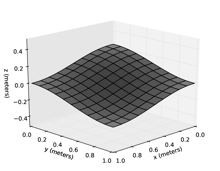
To demonstrate the numerical methods developed here, and the capabilities of the code implementing them, this section discusses the simulation of an acoustic pulse in brine striking an undulating bed of orthotropic layered sandstone. The surface of the bed is defined by

z_{\text{int}}(x,y)=z_{0}+H_{x}\cos\left(\frac{2\pi x}{L_{x}}\right)+H_{y}\cos\left(\frac{2\pi y}{L_{y}}\right),

(51)

with the parameters $z_{0}$ , $H_{x}$ , $L_{x}$ , $H_{y}$ , and $L_{y}$ given in Table 7. Figure 1 shows the surface. Below this $z$ coordinate, the domain is composed of the orthotropic sandstone of Table 2; above, it is composed of the brine from this sandstone. The curved interface between the two media is incorporated into the model using a mapped grid. At every point within the sandstone, the material’s plane of isotropy (the plane of the principal 1-2 axes) is parallel to the tangent plane of the surface above, in order to simulate a bed that has been folded, or deposited on a pre-existing uneven surface. In the simulation code, these variable principal axes are implemented by assigning constant material principal directions to each cell, equal to the directions evaluated at the cell centroid. The interface is taken to have open pores ( $\eta_{d}=1$ in interface condition (33)), and the incoming acoustic pulse propagates straight downward in the $-z$ direction. This problem exercises almost all of the capabilities of the three-dimensional code — it involves mapped grids, an orthotropic material with a variable principal direction, and a fluid-poroelastic interface.

Table 7: Surface and mapping parameters for demonstration problem. Note that the domain has horizontal dimensions

L_{x}/2

L_{y}/2

Surface parameter	$z_{0}$	$L_{x}$	$L_{y}$	$H_{x}$	$H_{y}$
Value	0 m	2 m	2 m	$\frac{3L_{x}}{16\pi}$	$\frac{3L_{y}}{16\pi}$
Mapping parameter	$z_{\text{bot}}$	$z_{\text{top}}$	$\xi_{\text{bot}}$	$\xi_{\text{int}}$	$\xi_{\text{top}}$	$r_{\text{bot}}$	$r_{\text{top}}$
Value	$-1$ m	0.5 m	0.15	0.6	0.9	$\frac{2}{\xi_{\text{bot}}}$	$\frac{2}{1-\xi_{\text{top}}}$

Refer to caption — Fig. 1: Brine-sandstone interface surface for demonstration problem.

The grid mapping for this problem is defined so that one of computational coordinate surfaces follows the interface, with the rest of the map chosen as a compromise between simplicity, smoothness, and the ability to have a flat grid plane at a useful distance below the interface to output slices of the solution for later plotting. The computational domain is the unit cube $[0,1]^{3}$ ; in the $xy$ plane, the problem’s symmetry allows the physical domain to be chosen as one quarter of a periodic tile of the surface, $[0,L_{x}/2]\times[0,L_{y}/2]$ . The grid mapping function in the horizontal axes is a simple scaling, $x:=\xi_{1}L_{x}/2$ and $y:=\xi_{2}L_{y}/2$ , while the mapping function for the $z$ coordinate is defined in terms of the horizontal physical coordinates $x$ and $y$ , and the vertical computational coordinate $\xi_{3}$ , as

z:=\begin{cases}z_{\text{bot}}+\frac{z^{\prime}_{\text{bot}}}{r_{\text{bot}}}\sinh r_{\text{bot}}(\xi_{3}-\xi_{\text{bot}}),&\xi_{3}<\xi_{\text{bot}}\\ z_{\text{bot}}+z^{\prime}_{\text{bot}}(\xi_{3}-\xi_{\text{bot}})+a_{\text{bot}}(x,y)\,b(\xi_{3};\xi_{\text{bot}}),&\xi_{\text{bot}}\leq\xi_{3}<\xi_{\text{int}}\\ z_{\text{top}}+z^{\prime}_{\text{top}}(\xi_{3}-\xi_{\text{top}})+a_{\text{top}}(x,y)\,b(\xi_{3};\xi_{\text{top}}),&\xi_{\text{int}}\leq\xi_{3}<\xi_{\text{top}}\\ z_{\text{top}}+\frac{z^{\prime}_{\text{top}}}{r_{\text{top}}}\sinh r_{\text{top}}(\xi_{3}-\xi_{\text{top}}),&\xi_{3}\geq\xi_{\text{top}},\end{cases}

(52)

where the derived quantities $z^{\prime}_{\text{bot}}$ , $z^{\prime}_{\text{top}}$ , $a_{\text{bot}}(x,y)$ , $a_{\text{top}}(x,y)$ , and $b(\xi_{3};\xi^{*})$ in the mapping function are defined by

\begin{gathered}\begin{aligned} z^{\prime}_{\text{bot}}&:=\frac{z_{0}-H_{x}-H_{y}-z_{\text{bot}}}{\xi_{\text{int}}-\xi_{\text{bot}}}&z^{\prime}_{\text{top}}&:=\frac{z_{\text{top}}-z_{0}-H_{x}-H_{y}}{\xi_{\text{top}}-\xi_{\text{int}}}\\ a_{\text{bot}}(x,y)&:=z_{\text{int}}(x,y)-(z_{0}-H_{x}-H_{y})&a_{\text{top}}(x,y)&:=z_{\text{int}}(x,y)-(z_{0}+H_{x}+H_{y})\end{aligned}\\ b(\xi_{3};\xi^{*}):=\frac{1}{2}\left(\sqrt{1+8\left(\frac{\xi_{3}-\xi^{*}}{\xi_{\text{int}}-\xi^{*}}\right)^{2}}-1\right).\end{gathered}

(53)

The values of the mapping parameters are given in Table 7.

The intent of the mapping (52) is to provide uniform grid spacings in the shortest grid columns above and below the interface, in order to prevent cells in these columns from being any smaller than necessary. The parameters $z^{\prime}_{\text{top}}$ and $z^{\prime}_{\text{bot}}$ are rates of change of $z$ with respect to $\xi_{3}$ in these shortest columns. Coordinates $z_{\text{top}}$ , $\xi_{\text{top}}$ , $z_{\text{bot}}$ , and $\xi_{\text{bot}}$ are the boundaries in physical and computational space of the part of the domain where the solution is considered “interesting.” Beyond these coordinates, the hyperbolic sine term smoothly stretches the grid in the vertical direction to move the boundaries of the computational domain further away from the interface, with the intent of improving the performance of the non-reflecting boundary conditions. The stretching will tend to blur the solution in the elongated cells, but this is acceptable because a high-quality solution is not required more than a little distance outside the region between $z_{\text{bot}}$ and $z_{\text{top}}$ . Note that for $\xi_{3}\leq\xi_{\text{bot}}$ and $\xi_{3}\geq\xi_{\text{top}}$ , surfaces of constant $\xi_{3}$ are horizontal planes. This is convenient for outputting a horizontal slice of the solution just below $z_{\text{bot}}$ for plotting. In the middle portion of the grid, the mapping is designed to have a continuous first derivative everywhere except at the sandstone-brine interface, in order to avoid any possible spurious internal reflections that might be caused by a nonsmooth mapping, and to improve accuracy in general. The mapping is allowed to be nonsmooth at the sandstone-brine interface because the second-order correction term is omitted there in any case, as in [31] — accuracy will already be degraded there, and requiring the mapping to be smooth at the interface would result in greater cell size variation elsewhere. Figure 2 shows the resulting grid. Note that the closely-spaced cells above the interface are not problematic for stability — since they are in the brine, not the sandstone, the wave speed within them is the acoustic wave speed of 1550 m/s, whereas the fast P wave speed in the sandstone is always at least 5260 m/s. The smallest vertical dimension of the cells above the interface is still over half the smallest vertical dimension below it, so stability is restricted by the fast P wave in the sandstone, not the acoustic wave in the brine.

By symmetry, the boundary conditions at the lateral faces of the domain are set to be reflective — for the faces parallel to the $yz$ plane, ghost cells are set to the value of the adjacent cell in the computational domain but with $\tau_{xz}$ , $\tau_{xy}$ , $v_{x}$ , and $q_{x}$ negated, while for the faces parallel to the $xz$ plane, $\tau_{yz}$ , $\tau_{xy}$ , $v_{y}$ , and $q_{y}$ are negated. Non-reflecting boundary conditions at the top and bottom face are implemented using zero-order extrapolation, with the elongation of the grid mapping near the top and bottom boundaries used to move these boundaries further away from the interface. Moving the boundaries further away allows the waves generated at the sandstone-brine interface to have angles of incidence closer to normal, which reduces reflections from this simple approach, and also postpones the arrival of waves at the boundary. The initial state is set to zero everywhere, except for the incoming plane wave, which is defined by its pressure field,

p_{\text{in}}(x,y,z):=\begin{cases}0.5\,\text{Pa}\left(1+\cos\left(\frac{2\pi(z-z_{0,\text{wave}})}{\lambda_{\text{wave}}}\right)\right),\quad&|z-z_{0,\text{wave}}|<\lambda_{\text{wave}}/2\\ 0,\quad&\text{otherwise},\end{cases}

(54)

where $z_{0,\text{wave}}=z_{0}+H_{x}+H_{y}+0.6\lambda_{\text{wave}}$ , $\lambda_{\text{wave}}=c_{\text{wave}}/f_{\text{wave}}$ , $c_{\text{wave}}$ is the sound speed in the brine (1550 m/s), and the fundamental frequency $f_{\text{wave}}$ is 10 kHz. To give a downward-propagating acoustic wave, the vertical fluid velocity is set to $q_{z}=-p_{\text{in}}/Z_{f}$ , where $Z_{f}$ is the acoustic impedance of the brine. The total simulation time is 400 $\mu$ s, and the dimensions of the grid used are $300\times 300\times 600$ cells. The MC limiter is used with all waves, with the full energy inner product wave strength ratio (46).

In order to obtain a solution more quickly, this demonstration problem was run in parallel using PetClaw. While there is a significant memory overhead associated with the PETSc distributed arrays used by PetClaw, as of this writing it is the only clawpack variant capable of running in parallel using dimensional splitting, which made it the only practical option in terms of run time for a large three-dimensional problem. With PetClaw the maximum memory footprint for the $300\times 300\times 600$ cell grid was roughly 105 GB. The problem was run on an Amazon EC2 CR1 high-memory cluster compute node, with 16 MPI processes; a total of 835 time steps were required, with a run time of 25.5 hours without viscosity included or 26.5 hours with viscosity, giving an aggregate throughput of roughly 30,000 cell time steps per CPU-second on the Intel Xeon E5-2670 CPUs used on this machine.

Figures 3 and 4 show the solution at time 399.9 $\mu$ s, the beginning of the final time step, with Figure 3 showing the solution without viscosity included and Figure 4 showing it with viscosity. The plots show an isometric view of the computational domain, with plots rendered on the $xz$ and $yz$ planes and on the horizontal plane at the $z$ coordinate of the centroids of the first layer of cells below $z=z_{\text{bot}}$ ; this is the highest layer of cells in the sandstone whose centroids all lie in a horizontal plane, so that a plot rendered on the surface defined by these centroids is easy to interpret. The plotted values on the $xz$ and $yz$ planes are generated by first projecting the values from the centroids of the layer of cells on that side of the domain to the appropriate plane, using the problem symmetry — that is, for values on the $xz$ plane, $\tau_{yz}$ , $\tau_{xy}$ , $v_{y}$ , and $q_{y}$ are set to zero, while for values on the $yz$ plane, $\tau_{xz}$ , $\tau_{xy}$ , $v_{x}$ , and $q_{x}$ are set to zero. The locations associated with these values for plotting purposes are the orthogonal projections of the corresponding cell centroids onto the axis planes. The problem symmetry is also used to extend the computed solution to the lateral corners of the computational domain – values at $(x,y)=(0,0)$ , $(L_{x}/2,0)$ , $(0,L_{y}/2)$ , and $(L_{x}/2,L_{y}/2)$ are obtained by copying the values at the nearest cells, then setting all the shear stresses and horizontal velocity components to zero. In addition, since computing the energy density requires knowing the material principal directions, the principal directions on the $xz$ and $yz$ faces are computed at the points on these planes associated with the projected values, not the original cell centroids. Values plotted in the horizontal plane near the bottom of the domain are associated with the $z$ coordinate of the cell centroids, which is $-1.0014$ m; this is the $z$ coordinate of the plane shown.

The solution of this demonstration problem is quite complex, but there are a number of clearly recognizable features. For the inviscid case, Figure 3a, which shows the energy density, provides a broad view with most of the solution features identifiable. At the bottom, the light arc across the horizontal slice and stretching up into the lower parts of the sides of the domain is the initial fast P wave created when the acoustic wave struck the peak of the sandstone. The additional arc sweeping up and inward from the intersection of the fast P wave with the domain edge is the same initial fast P wave reflected off the boundary. Further inward toward the $z$ axis, the light diagonal bands are shear waves originating from the acoustic wave striking the flanks of the sandstone peak. Just below the surface, the slow P wave is clearly visible as a narrow bright band; because the pore structure is open at the surface, a strong slow P wave is excited by the incident acoustic wave. Finally, above the surface, the incident wave has been reflected and has already partially left the computational domain. Figure 3b shows some numerical artifacts in the low-pressure region at the very top of the domain, but these are outside the designated area of interest for the problem.

For the viscous case, the solution is generally similar, but the slow P wave is almost entirely suppressed by the viscous dissipation. It is, however, faintly visible as a band of increased pressure just under the surface in Figure 4b. Comparing the energy density plots of Figures 3a and 4a, the fast P and S waves are also somewhat dissipated and slowed by viscosity, although the vertical direction stress fields (Figures 3c and 4c) are hardly affected aside from the loss of the slow P wave.

5 Summary and future work

This paper has covered the extension of the finite volume wave propagation methods for poroelasticity developed in [31] and [32] to three dimensions. Section 2 covered the development of a first-order linear hyperbolic system of PDEs describing three-dimensional Biot theory at low frequencies. An energy density functional $\mathcal{E}$ was developed for the three-dimensional system, and as in [32] $\mathcal{E}$ was found to be a strictly convex entropy function of the system in the sense of Chen, Levermore, and Liu [13]. Interface conditions for coupling fluid and poroelastic media were also exhibited.

Section 3 discussed the implementation of high-resolution finite volume methods for fluid-poroelastic problems on mapped grids in three dimensions. The complications associated with defining cell face normals on an arbitrary hexahedral grid were discussed, and a technique was developed for defining suitable normal vectors for a finite volume scheme. The solution procedure for poroelastic-fluid and poroelastic-poroelastic Riemann problems with interface conditions developed in [31] was also extended to three dimensions. In addition, a new strength ratio for wave limiting was developed for three-dimensional poroelasticity, which avoided the problems with ambiguous shear wave polarization directions that would otherwise be encountered; besides avoiding the inappropriate suppression of higher-order terms that could be encountered with the traditional wave strength ratio calculation, the new limiting approach also gave a modest reduction in error for most cases when applied to the cylindrical scatterer test problems of [31].

With all the algorithmic pieces in place, Section 4 applied the methods of Section 3 to some test problems to verify their effectiveness. The first test problems were simple plane waves, for which the numerical solution could easily be compared to an analytical solution for the same problem. Due to the use of dimensional splitting, only first-order accuracy could be achieved in the general case of waves propagating obliquely to the grid, although when the wavevector was aligned with the grid axes second-order convergence was achieved, consistent with previous results [31, 32]. A special set of test problems was then run to demonstrate the new $\mathbf{E}$ -limiter on a problem of the type it was developed for, where the different polarizations of shear wave switch order in the Riemann solution output; the $\mathbf{E}$ -limiter gave a modest reduction in 1-norm error, and a substantial reduction — up to a factor of five — in max-norm error. A more complex demonstration problem involving an acoustic wave in brine striking a periodically undulating bed of sandstone was also run. This problem was intended to exercise as many capabilities of the simulation code as possible, and included a fluid-poroelastic interface, an orthotropic poroelastic medium with continuously varying principal axes, and a non-rectilinear mapped grid designed to conform to the uneven surface of the sandstone bed. Results for this demonstration problem were quite complex, with waves of all three types visible, but the simulation code handled it without difficulty.

There are many opportunities for extension of the work presented here. The most obvious route for improvement would be the replacement of the dimensional splitting scheme with a more accurate method. While extending the transverse propagation scheme from [31] into three dimensions would require an inordinate number of transverse Riemann solutions, a more promising approach would be to use the SharpClaw package of Ketcheson et al. [28], which employs a semidiscrete approach. Switching to a semidiscrete scheme would also allow the use of an exponential integrator [25], which may allow better accuracy in the stiff regime identified in [32]. Another opportunity to build upon this work would be extension to higher frequencies — the numerical scheme used here could be extended in a straightforward fashion to include additional memory variables to model a frequency-dependent kernel used to generalize Darcy’s law to higher frequencies [34].

In order to facilitate reproduction of these results, all the code used to produce them has been archived at http://dx.doi.org/10.6084/m9.figshare.783056.

6 Acknowledgements

This work has benefited greatly from the direct input and advice of Prof. Randall J. LeVeque of the Department of Applied Mathematics, University of Washington, as well as from the clawpack simulation framework. The author also wishes to thank Prof. M. Yvonne Ou of the University of Delaware, who introduced him to poroelasticity theory and whose help has been invaluable in understanding the mechanics of porous media. In addition, the treatment of mapped grids in three dimensions in Section 3.1, particularly the appropriate handling of face areas and normals, was inspired by correspondence with Prof. Donna Calhoun of Boise State University.

This work was funded in part by NIH grant 5R01AR53652-2, and by NSF grants DMS-0914942 and DMS-1216732.

References

[1] D. F. Aldridge, N. P. Symons, and L. C. Bartel, Poroelastic wave propagation with a velocity-stress-pressure algorithm, in Poromechanics III, 2005, pp. 253–258.
[2] A. Alghamdi, A. Ahmadia, D. I. Ketcheson, M. G. Knepley, K. T. Mandli, and L. Dalcin, Petclaw: A scalable parallel nonlinear wave propagation solver for python, in Proceedings of the 19th High Performance Computing Symposia, Society for Computer Simulation International, 2011, pp. 96–103.
[3] K. Attenborough, D. L. Berry, and Y. Chen, Acoustic scattering by near-surface inhomogeneities in porous media., tech. report, Defense Technical Information Center OAI-PMH Repository [http://stinet.dtic.mil/oai/oai] (United States), 1998.
[4] D. S. Bale, R. J. LeVeque, S. Mitran, and J. A. Rossmanith, A wave propagation method for conservation laws and balance laws with spatially varying flux functions, SIAM Journal on Scientific Computing, 24 (2002), pp. 955–978.
[5] M. A. Biot, Theory of propagation of elastic waves in a fluid-saturated porous solid. I. Low-frequency range, Journal of the Acoustical Society of America, 28 (1956), pp. 168–178.
[6] , Theory of propagation of elastic waves in a fluid-saturated porous solid. II. Higher frequency range, Journal of the Acoustical Society of America, 28 (1956), pp. 179–191.
[7] , Mechanics of deformation and acoustic propagation in porous media, Journal of Applied Physics, 33 (1962), pp. 1482–1498.
[8] J. L. Buchanan and R. P. Gilbert, Determination of the parameters of cancellous bone using high frequency acoustic measurements, Mathematical and Computer Modelling, 45 (2007), pp. 281–308.
[9] , Determination of the parameters of cancellous bone using high frequency acoustic measurements II: inverse problems, Journal of Computational Acoustics, 15 (2007), pp. 199–220.
[10] J. L. Buchanan, R. P. Gilbert, and K. Khashanah, Determination of the parameters of cancellous bone using low frequency acoustic measurements, Journal of Computational Acoustics, 12 (2004), pp. 99–126.
[11] J. L. Buchanan, R. P. Gilbert, A. Wirgin, and Y. S. Xu, Marine acoustics: direct and inverse problems, SIAM, Philadelphia, 2004.
[12] J. M. Carcione, Wave Fields in Real Media: Wave Propagation in Anisotropic, Anelastic, and Porous Media, Elsevier, Oxford, 2001.
[13] G.-Q. Chen, C. D. Levermore, and T.-P. Liu, Hyperbolic conservation laws with stiff relaxation terms and entropy, Communications in Pure and Applied Mathematics, 47 (1994), pp. 787–830.
[14] G. Chiavassa and B. Lombard, Wave propagation across acoustic/Biot’s media: a finite-difference method, Communications in Computational Physics, 13 (2013), pp. 985–1012.
[15] S. C. Cowin, Bone poroelasticity, Journal of Biomechanics, 32 (1999), pp. 217–238.
[16] S. C. Cowin and L. Cardoso, Fabric dependence of bone ultrasound, Acta of Bioengineering and Biomechanics, 12 (2010).
[17] N. Dai, A. Vafidis, and E. Kanasewich, Wave propagation in heterogeneous porous media: a velocity-stress, finite-difference method, Geophysics, 60 (1995), pp. 327–340.
[18] J. de la Puente, M. Dumbser, M. Käser, and H. Igel, Discontinuous Galerkin methods for wave propagation in poroelastic media, Geophysics, 73 (2008), pp. T77–T97.
[19] G. Degrande and G. De Roeck, FFT-based spectral analysis methodology for one-dimensional wave propagation in poroelastic media, Transport in Porous Media, 9 (1992), pp. 85–97.
[20] E. Detournay and A. H.-D. Cheng, Poroelastic response of a borehole in a non-hydrostatic stress field, International Journal of Rock Mechanics and Mining Sciences and Geomechanics Abstracts, 25 (1988), pp. 171–182.
[21] S. K. Garg, A. H. Nayfeh, and A. J. Good, Compressional waves in fluid-saturated elastic porous media, Journal of Applied Physics, 45 (1974), pp. 1968–1974.
[22] R. P. Gilbert, P. Guyenne, and M. Y. Ou, A quantitative ultrasound model of the bone with blood as the interstitial fluid, Mathematical and Computer Modelling, 55 (2012), pp. 2029–2039.
[23] R. P. Gilbert and Z. Lin, Acoustic field in a shallow, stratified ocean with a poro-elastic seabed, Zeitschrift für Angewandte Mathematik und Mechanik, 77 (1997), pp. 677–688.
[24] R. P. Gilbert and M. Y. Ou, Acoustic wave propagation in a composite of two different poroelastic materials with a very rough periodic interface: a homogenization approach, International Journal for Multiscale Computational Engineering, 1 (2003), pp. 431–440.
[25] M. Hochbruck and A. Ostermann, Exponential integrators, Acta Numerica, 19 (2010), pp. 209–286.
[26] F. Kemm, A comparative study of TVD-limiters – well-known limiters and an introduction of new ones, International Journal for Numerical Methods in Fluids, 67 (2011), pp. 404–440.
[27] D. I. Ketcheson, K. Mandli, A. J. Ahmadia, A. Alghamdi, M. Q. de Luna, M. Parsani, M. G. Knepley, and M. Emmett, Pyclaw: Accessible, extensible, scalable tools for wave propagation problems, SIAM Journal on Scientific Computing, 34 (2012), pp. C210–C231.
[28] D. I. Ketcheson, M. Parsani, and R. J. LeVeque, High-order wave propagation algorithms for hyperbolic systems, SIAM Journal on Scientific Computing, 35 (2013), pp. A351–A377.
[29] J. O. Langseth and R. J. LeVeque, A wave propagation method for three-dimensional hyperbolic conservation laws, Journal of Computational Physics, 165 (2000), pp. 126–166.
[30] G. I. Lemoine, Numerical modeling of poroelastic-fluid systems using high-resolution finite volume methods, PhD thesis, University of Washington, 2013.
[31] G. I. Lemoine and M. Y. Ou, Finite volume modeling of poroelastic-fluid wave propagation with mapped grids. http://arxiv.org/abs/1305.2952, 2013.
[32] G. I. Lemoine, M. Y. Ou, and R. J. LeVeque, High-resolution finite volume modeling of wave propagation in orthotropic poroelastic media, SIAM Journal on Scientific Computing, 35 (2013), pp. B176–B206.
[33] R. J. LeVeque, Finite Volume Methods for Hyperbolic Problems, Cambridge University Press, New York, 2002.
[34] J.-F. Lu and A. Hanyga, Wave field simulation for heterogeneous porous media with singular memory drag force, Journal of Computational Physics, 208 (2005), pp. 651–674.
[35] B. G. Mikhailenko, Numerical experiment in seismic investigations, Journal of Geophysics, 58 (1985), pp. 101–124.
[36] C. Morency and J. Tromp, Spectral-element simulations of wave propagation in porous media, Geophysical Journal International, 179 (2008), pp. 1148–1168.
[37] A. Naumovich, On finite volume discretization of the three-dimensional Biot poroelasticity system in multilayer domains, Computational Methods in Applied Mathematics, 6 (2006), pp. 306–325.
[38] J. E. Santos and E. J. Oreña, Elastic wave propagation in fluid-saturate porous media, part II: The Galerkin procedures, Mathematical Modeling and Numerical Analysis, 20 (1986), pp. 129–139.

Three-Dimensional Mapped-Grid Finite Volume Modeling of Poroelastic-Fluid Wave Propagation11 1 Much of this work comes from Section 2.2 and Chapters 8 and 9 of [30]. This is the first widely-distributed version.