Viable $f(T)$ models are practically indistinguishable from $\Lambda$CDM

The $\Lambda$CDM model is currently the simplest model consistent with practically all cosmological observations. It assumes homogeneity and isotropy on large cosmological scales and the presence of a cosmological constant $\Lambda$ in the context of general relativity. Despite of its simplicity and its overall consistency with observations, $\Lambda$CDM has two weak points:

1. 1.

   It requires a theoretically unnatural and fine-tuned value for $\Lambda$.

2. 2.

   It is marginally consistent with some recent large scale cosmological observations (for instance the cosmic microwave background anomalies).

Motivated by these two weak points, a wide range of more complex generalized cosmological models has been investigated. Most of these models reduce to $\Lambda$CDM for specific values of their parameters. They can be classified in two broad classes: Modified gravity models constitute the one class (see for instance [1]), with the other being the scalar field dark energy that adheres to general relativity (see for instance [2, 3]). Among the variety of modified gravity theories, $f(T)$ gravity has recently gained a lot of attention. It is based on the old formulation of the teleparallel equivalent of general relativity (TEGR) [4, 5, 6]. In teleparallel formulations the dynamical fields are the four linearly independent vierbeins, while one uses the curvatureless Weitzenböck connection instead of the torsionless Levi-Civita one. Thus, one can construct the torsion tensor, which includes all the information concerning the gravitational field, and then by suitable contractions one can write down the corresponding Lagrangian density $T$ [5] (assuming invariance under general coordinate transformations, global Lorentz and parity transformations, and requiring up to second-order terms of the torsion tensor). Finally, $f(T)$ gravity arises as a natural extension of TEGR, if one generalizes the Lagrangian to be a function of $T$ [7, 8, 9], inspired by the well-known extension of $f(R)$ Einstein-Hilbert action. However, the significant advantage is that although the curvature tensor contains second-order derivatives of the metric and thus $f(R)$ gravity gives rise to fourth-order equations which may lead to pathologies, the torsion tensor includes only products of first derivatives of the vierbeins, giving rise to second-order field equations.

Although TEGR coincides completely with general relativity both at the background and perturbation levels, $f(T)$ gravity exhibits novel structural and phenomenological features. In particular, imposing a cosmological background one can extract various cosmological solutions, consistent with the observable behavior [7, 8, 9, 10, 11, 12, 13]. Additionally, imposing spherical geometry one can investigate the spherical, black-hole solutions of $f(T)$ gravity [14]. However, we stress that although TEGR coincides with GR, $f(T)$ gravity does not coincide with $f(R)$ extension, but it rather constitutes a different class of modified gravity.

One crucial question is what classes of $f(T)$ extensions are allowed by observations. At the theoretical level, the aforementioned cosmological and spherical solutions lead to a variety of such expressions. However, taking into account observational data, either from cosmological [11, 12, 15, 16] as well as from Solar System observations [13], one can show that the deviations from TEGR must be small.

In the present work we are interested in constraining the $f(T)$ forms using the latest cosmological data, both at the background and perturbation levels. In order to do so we need to define the Hubble parameter as a function of redshift. The issue of using iterative techniques in order to treat the Hubble expansion in $f(R)$ gravity has been proposed by Starobinsky in Ref. [17]. Furthermore, in a recent paper some of us [18] used a new iterative approach in order to observationally constrain deviations of $f(R)$ models from $\Lambda$CDM and general relativity. In this context, we first showed that all known viable $f(R)$ models may be written as perturbations around $\Lambda$CDM with a deviation parameter we called $b$ (for $b=0$ these models reduce to $\Lambda$CDM). Using a novel perturbative iterative technique we were able to construct analytic cosmological expansion solutions of a highly nonlinear and stiff system of ordinary differential equations and impose cosmological observational constraints on the deviation parameter $b$.

We also showed that the observationally viable $f(R)$ models effectively include the cosmological constant even though they were proposed as being free from a cosmological constant in the original $f(R)$ papers [19, 17]. Inspired by our previous similar work on $f(R)$ gravity [18], we extend it to the case of $f(T)$ gravity models and use the standard joint likelihood analysis of the recent supernovae type Ia data (SnIa), the cosmic microwave background (CMB) shift parameters, the baryonic acoustic oscillations (BAO) and the growth rate data provided by the various galaxy surveys. Based on these cosmological observations we identify the viable range of parameters of five previously proposed $f(T)$ models. Additionally, comparing the resulting analytical expressions of the $f(T)$ Hubble parameter with the numerical solutions at low and intermediate redshifts, we verify that our iterative perturbative technique is highly accurate.

The plan of the work is as follows: In Sec. II we briefly discuss the main properties of the $f(T)$ gravity, while in Sec. III we apply the $f(T)$ gravity in a cosmological framework, providing the relevant equations both at the background and perturbation levels. In Sec. IV we present and we analytically elaborate on all the $f(T)$ models of the literature with two parameters (out of which one is independent). In Sec. V we impose observational constraints, utilizing three parametrizations of the growth index. Finally, the main conclusions are summarized in Sec. VI.

In this section we briefly review the $f(T)$ gravitational paradigm. In this construction the dynamical variables are the vierbein fields ${\mathbf{e}_{A}(x^{\mu})}$ ¹¹ 1 Throughout the manuscript, greek indices $\mu,\nu,$… and capital Latin indices $A,B,$… run over all coordinate and tangent space-time 0, 1, 2, 3, while lower case latin indices (from the beginning of the alphabet) $a,b,$… and lower case latin indices (from the middle of the alphabet) $i,j,...$, run over tangent-space and spatial coordinates 1, 2, 3 respectively.. The vierbeins at each point $x^{\mu}$ of the manifold form an orthonormal basis for the tangent space, that is $\mathbf{e}_{A}\cdot\mathbf{e}_{B}=\eta_{AB}$, with $\eta_{AB}={\rm diag}(1,-1,-1,-1)$, and they can be expressed in terms of the components $e_{A}^{\mu}$ in a coordinate basis as $\mathbf{e}_{A}=e^{\mu}_{A}\partial_{\mu}$. Therefore, the metric tensor is obtained from the dual vierbein through

While in usual gravitational formalism one uses the torsionless Levi-Civita connection, in the present formulation one uses the curvatureless Weitzenböck connection defined as $\overset{\mathbf{w}}{\Gamma}^{\lambda}_{\nu\mu}\equiv e^{\lambda}_{A}\>\partial_{\mu}e^{A}_{\nu}$ [20], and the corresponding torsion tensor is written as

Furthermore, the contorsion tensor, which provides the difference between Weitzenböck and Levi-Civita connections, is given by $K^{\mu\nu}_{\>\>\>\>\rho}\equiv-\frac{1}{2}\Big(T^{\mu\nu}_{\>\>\>\>\rho}-T^{\nu\mu}_{\>\>\>\>\rho}-T_{\rho}^{\>\>\>\>\mu\nu}\Big)$, while for convenience we define $S_{\rho}^{\>\>\>\mu\nu}\equiv\frac{1}{2}\Big(K^{\mu\nu}_{\>\>\>\>\rho}+\delta^{\mu}_{\rho}\>T^{\alpha\nu}_{\>\>\>\>\alpha}-\delta^{\nu}_{\rho}\>T^{\alpha\mu}_{\>\>\>\>\alpha}\Big)$. Finally, imposing coordinate, Lorentz and parity symmetries, and the additional requirement the Lagrangian to be second order in the torsion tensor [5, 6], one obtains the teleparallel Lagrangian (called “torsion scalar” too)

Thus, in the teleparallel gravitational paradigm, all the information concerning the gravitational field is embedded in the torsion tensor ${T}^{\lambda}_{\>\mu\nu}$, which produces the torsion scalar $T$ in a similar way as the curvature Riemann tensor gives rise to the Ricci scalar in standard general relativity.

In the teleparallel equivalent of general relativity the action is just $T$. However, one can be inspired by the $f(R)$ extensions of general relativity and extend $T$ to a function $T+f(T)$. Therefore, the corresponding action of $f(T)$ gravity reads as

where $e=\text{det}(e_{\mu}^{A})=\sqrt{-g}$, $G_{N}$ is the gravitational constant, and we use units where the light speed is equal to 1. Lastly, TEGR and thus general relativity is restored when $f(T)=0$, while if $f(T)=$ const we recover general relativity with a cosmological constant.

We now proceed to the cosmological application of $f(T)$ gravity. In order to construct a realistic cosmology we have to incorporate in the action the matter and the radiation sectors respectively. Therefore, the total action is written as

where the matter and radiation Lagrangians are assumed to correspond to perfect fluids with energy densities $\rho_{m}$, $\rho_{r}$ and pressures $P_{m}$, $P_{r}$ respectively.

Secondly, in order to examine a universe governed by $f(T)$ gravity, we have to impose the usual homogeneous and isotropic geometry. Therefore, we consider the common choice for the vierbien form, that is,

which corresponds to a flat Friedmann-Robertson-Walker (FRW) background geometry with metric

with $a(t)$ the scale factor.

In this section we review all the specific $f(T)$ models that have appeared in the literature, with two parameters out of which one is independent. We calculate the function $y(z,{\bf r})$ using (18) and their $G_{\rm eff}(a)$ using (32). We quantify the deviation of the function $y(z,{\bf r})$ from its $\Lambda$CDM value (constant) through a distortion parameter $b$. The considered models are as follows.

1. 1.

   The power-law model of Bengochea and Ferraro (hereafter $f_{1}$CDM) [8], with

   $$f(T)=\alpha(-T)^{b},$$

   (33)

   where $\alpha$ and $b$ are the two model parameters. Substituting this $f(T)$ form into the modified Friedmann equation (9) at present, we obtain

   $\displaystyle\alpha=(6H_{0}^{2})^{1-b}\frac{\Omega_{F0}}{2b-1},$

   (34)

   while (18) gives

   $$y(z,b)=E^{2b}(z,b)\;.$$

   (35)

   Additionally, the effective Newton’s constant from (32) becomes

   $$G_{\rm eff}(z)=\frac{G_{N}}{1+\frac{b\Omega_{F0}}{(1-2b)E^{2(1-b)}}}\;.$$

   (36)

   It is evident that for $b$ strictly equal to zero the $f_{1}$CDM model reduces to $\Lambda$CDM cosmology, namely $T+f(T)=T-2\Lambda$ (where $\Lambda=3\Omega_{F0}H_{0}^{2}$, $\Omega_{F0}=\Omega_{\Lambda 0}$), while for $b=1/2$ it reduces to the Dvali, Gabadadze and Porrati (DGP) ones [33]. Note that in order to obtain an accelerating expansion, it is required that $b<1$.

2. 2.

   The Linder model (hereafter $f_{2}$CDM) [9]

   $\displaystyle f(T)=\alpha T_{0}(1-e^{-p\sqrt{T/T_{0}}}),$

   (37)

   with $\alpha$ and $p$ the two model parameters. In this case from (9) we find that

   $\displaystyle\alpha=\frac{\Omega_{F0}}{1-(1+p)e^{-p}}\;,$

   (38)

   and from (18) we acquire

   $$y(z,p)=\frac{1-(1+pE)e^{-pE}}{1-(1+p)e^{-p}}\;,$$

   (39)

   while from (32) we obtain

   $$G_{\rm eff}(z)=\frac{G_{N}}{1+\frac{\Omega_{F0}p~e^{-pE}}{2E[1-(1+p)e^{-p}]}}\;.$$

   (40)

   Thus, for $p\rightarrow+\infty$ the $f_{2}$CDM reduces to $\Lambda$CDM cosmology, since

   $$\lim_{p\rightarrow+\infty}[T+f(T)]=T-2\Lambda\;.$$

   (41)

   The parameter $p$ of the present $f_{2}$CDM model has a different interpretation comparing to $b$ for the $f_{1}$CDM model, since the two models are obviously different. However, since in the limiting case they both reduce to $\Lambda$CDM paradigm, we can rewrite the present $f_{2}$CDM model replacing $p=1/b$. In this case (39) leads to

   $$y(z,b)=\frac{1-(1+\frac{E}{b})e^{-E/b}}{1-(1+\frac{1}{b})e^{-1/b}},$$

   (42)

   which indeed tends to unity for $b\rightarrow 0^{+}$.

3. 3.

   Motivated by exponential $f(R)$ gravity [48], one can construct the following $f(T)$ model (hereafter $f_{3}$CDM):

   $\displaystyle f(T)=\alpha T_{0}(1-e^{-pT/T_{0}}),$

   (43)

   with $\alpha$ and $p$ the two model parameters. In this case we obtain

   $\displaystyle\alpha=\frac{\Omega_{F0}}{1-(1+2p)e^{-p}}\;,$

   (44)

   $$y(z,p)=\frac{1-(1+2pE^{2})e^{-pE^{2}}}{1-(1+2p)e^{-p}}\;.$$

   (45)

   and

   $$G_{\rm eff}(z)=\frac{G_{N}}{1+\frac{\Omega_{F0}p~e^{-pE^{2}}}{1-(1+2p)e^{-p}}}\;.$$

   (46)

   Similarly to the previous case we can rewrite $f_{3}$CDM model using $p=1/b$, obtaining

   $$y(z,b)=\frac{1-(1+\frac{2E^{2}}{b})e^{-E^{2}/b}}{1-(1+\frac{2}{b})e^{-1/b}}\;.$$

   (47)

   Again, we see that for $p\rightarrow+\infty$, or equivalently for $b\rightarrow 0^{+}$, the $f_{3}$CDM model tends to the $\Lambda$CDM cosmology.

4. 4.

   The Bamba et al. logarithmic model (hereafter $f_{4}$CDM) [49]

   $\displaystyle f(T)=\alpha T_{0}\sqrt{\frac{T}{qT_{0}}}\;{\rm ln}\left(\frac{qT_{0}}{T}\right)$

   (48)

   with $\alpha$ and $q$ the two model parameters. In this case we obtain

   $\displaystyle\alpha=\frac{\Omega_{F0}\sqrt{q}}{2}\;,$

   (49)

   $$y(z)=E(z)\;,$$

   (50)

   and

   $\displaystyle G_{\rm eff}(z)=\frac{G_{N}}{1+\frac{\Omega_{F0}}{2E}\left[\ln\left(\frac{\sqrt{q}}{E}\right)-1\right]}.$

   (51)

   The fact that the distortion function does not depend on the model parameters, allows us to write (16) as

   	$\displaystyle E(z)$	$\displaystyle=$	$\displaystyle\frac{1}{2}\sqrt{\Omega^{2}_{F0}+4\left[\Omega_{m0}(1+z)^{3}+\Omega_{r0}(1+z)^{4}\right]}$		(52)
   		$\displaystyle+$	$\displaystyle\frac{\Omega_{F0}}{2}.$

   Interestingly enough, from the above relation we deduce that at the background level the $f_{4}$CDM model coincides with the flat DGP one (with $\Omega_{F0}=\Omega_{DGP}$), which implies that the two nonstandard gravity models are cosmologically equivalent as far as the cosmic expansion is concerned, in spite of the fact that the two models have a completely different geometrical basis. At the perturbative level, however, we do expect to find differences between $f_{4}$CDM and DGP, since $G_{\rm eff}(z)$ evolves differently in two models [in flat DGP gravity we have $\frac{G_{\rm eff}(z)}{G_{N}}=\frac{2+4\Omega^{2}_{m}(z)}{3+3\Omega^{2}_{m}(z)}$].

   Notice that this model does not give $\Lambda$CDM cosmology for any value of its parameters. However, in this work we are interested in the viable $f(T)$, in the sense that these $f(T)$ models can describe the matter and dark energy eras as well as they are consistent with the observational data (including Solar System tests), and finally they have stable perturbations. Although these necessary analysis have not yet been performed for all the above $f(T)$ models, a failure of a particular model to pass one of these is enough to exclude it. Therefore, since the present $f_{4}$CDM model coincides with DGP at the background level, it inherits its disadvantages concerning the confrontation with observations. Thus, as anticipated from previous studies [50], we verify in the following section that this model is nonviable when tested using the latest cosmological observations.

5. 5.

   The hyperbolic-tangent model (hereafter $f_{5}$CDM) [51]

   $\displaystyle f(T)=\alpha(-T)^{n}{\rm tanh}\left(\frac{T_{0}}{T}\right)$

   (53)

   with $\alpha$ and $n$ the two model parameters. In this case we obtain

   $\displaystyle\alpha=-\frac{\Omega_{F0}(6H_{0})^{1-n}}{\left[2{\rm sech}^{2}(1)+(1-2n){\rm tanh}(1)\right]}\;,$

   (54)

   $\displaystyle y(z,n)=E^{2(n-1)}\frac{2{\rm sech}^{2}\left(\frac{1}{E^{2}}\right)+(1-2n)E^{2}{\rm tanh}\left(\frac{1}{E^{2}}\right)}{2{\rm sech}^{2}(1)+(1-2n){\rm tanh}(1)}$

   (55)

   and

   $\displaystyle G_{\rm eff}(z)=\frac{G_{N}}{1+\frac{\Omega_{F0}E^{2(n-2)}\left[nE^{2}{\rm tanh}\left(\frac{1}{E^{2}}\right)-{\rm sech}^{2}\left(\frac{1}{E^{2}}\right)\right]}{2{\rm sech}^{2}(1)+(1-2n){\rm tanh}(1)}}.$

   (56)

   The $f_{5}$CDM model does not give $\Lambda$CDM cosmology for any value of its parameters. However, as we show in the next section, this model is in mild tension with the data as it has a best fit $\chi_{min}^{2}=(579.583,580.723,578.027)$ for the $\Gamma_{0}$, $\Gamma_{1}$ and $\Gamma_{2}$ growth rate parameterizations respectively, which is significantly larger than that of $f_{1-3}$CDM and $\Lambda$CDM models respectively (see Table 1). Additionally the current $f(T)$ model has one more free parameter. For the reasons developed above we consider it as nonviable (see also akaike information criterion (AIC) test in Table I.)

The above five $f(T)$ forms are the ones that have been used in the literature of $f(T)$ cosmology, possessing up to two parameters, out of which one is independent. Clearly, in principle one could additionally consider their combinations too; however, the appearance of many free parameters would be a significant disadvantage. Therefore, in the present work we focus only on these five elementary Ansätze.

As we showed, for the first three the distortion parameter measures the smooth deviation from the $\Lambda$CDM model. The other two models do not have $\Lambda$CDM cosmology as a limiting case; however, as we show in the next section, they are in tension with observations. Thus, in the rest of this section we focus on the first three models, namely on $f_{1-3}$CDM ones.

Having performed the above elaboration of various $f(T)$ models, we can now follow the procedure and iterative techniques of Basilakos, Nesseris and Perivolaropoulos [18], in which we have shown that all the observationally viable $f(R)$ parameterizations can be expressed as perturbations deviating from $\Lambda$CDM cosmology.

For the $f_{1}$CDM model there are two different, but complementary, ways we can find analytical approximations for the Hubble parameter. The first method involves doing a Taylor expansion of $E^{2}(z,b)$ around $b=0$, while in the second we perform the Taylor expansion in the modified Friedman equation directly. Below, we briefly review and test both methods, called $M_{1}$ and $M_{2}$ respectively.

First, from (16) with (35) we can write explicitly the Hubble parameter for the $f_{1}$CDM model as

where

Obviously, in Eq. (57) if we set $b$ strictly equal to zero then we get the Hubble parameter for the $\Lambda$CDM model

Now, performing a Taylor expansion, up to second order, on $E^{2}(z,b)$ around $b=0$ and with the help of (57) we arrive at

The terms involving the derivatives of $y(z,b)$ can readily be calculated from Eq. (58) as

and evaluating the above equation for $b=0$ we have

Similarly for the second derivative term we have

Thus, the Taylor expansion up to second order for the first method $M_{1}$ becomes

The second method $M_{2}$ involves performing a Taylor expansion in the modified Friedman equation (57) directly. For the details in this case we refer the interested reader to the Appendix and just present the result here:

where $\mathcal{W}_{k}(\omega)$ is the Lambert function defined via $\omega\equiv\mathcal{W}_{k}(\omega)e^{\mathcal{W}_{k}(\omega)}$ for all complex numbers $\omega$. The Lambert function has branch-cut discontinuities, so the different branches are indicated by the integer $k$. Our solution has $k=0$ (the principal branch) for $b\leq 0$ and $k=-1$ for $b>0$.²² 2 The Lambert function $\mathcal{W}_{k}(\omega)$ is defined in Mathematica as ProductLog$\left[k,\omega\right]$ and can be evaluated to arbitrary precision for integer values of $k$ and real or complex values of $\omega$..

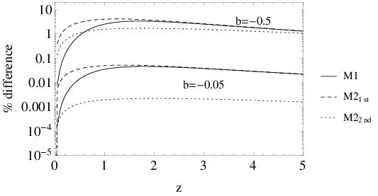
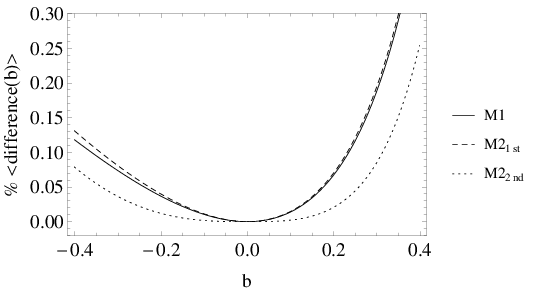
In order to examine the accuracy of the approximations of (64) and (65), we calculate the average percent deviation from the exact numerical solution of (57), defined as

where the average is taken over redshifts in the range $z\in[0,100]$. In Fig. 1 we show the corresponding results. In particular, on the left plot we show the percent difference between the numerical solution of Eqs. (16) and (35) and the analytical approximations of Eqs. (64) and (65) as a function of $z$, for various values of the parameter $b$ for both methods $M_{1}$, at first (dashed line) and second order (dotted line) and $M_{2}$ (solid black line). As it can be seen, at redshifts $z\lesssim 2$ method $M_{2}$ is significantly better than the first-order $M_{1}$, but overall, obviously the second-order method $M_{2}$ is much better than the other two.

On the right plot we show the average percent difference $\langle\textrm{difference}(b)\rangle$ between the numerical solution of Eqs. (16) and (35) and the analytical approximations of Eqs. (64) and (65) as a function of the parameter $b$. In this case, the average over the redshift is taken in the range $z\in[0,100]$. Clearly, on average the second-order method is significantly better than the other two methods, the first-order $M_{1}$ and the $M_{2}$. Thus, we conclude that the second order series expansion of Eq. (64) around $\Lambda$CDM for the $f_{1}$CDM model is a very good approximation, especially for realistic values of the parameter $b$.

Unfortunately, for the $f_{2}$CDM and $f_{3}$CDM models it is not possible to analytically obtain similar expressions, due to the presence of terms like $\sim e^{-1/b}$, which do not admit a Taylor expansion around $b\sim 0$. However, as mentioned earlier, they both have the $\Lambda$CDM model as a limit for $b\rightarrow 0^{+}$.

In this section we perform a complete and detailed observational analysis of the above five $f(T)$ models. In particular, we implement a joint statistical analysis with the appropriate Akaike information criterion [52], involving the latest expansion data (SnIa [53], BAO [54, 55] and the 9-year WMAP CMB shift parameter [56]) and the growth data (as collected by [18]). The likelihood analysis, the Akaike information criterion, the expansion data, the growth data and the corresponding covariances can be found in Table I and Sec. IV of our previous work [18]. Moreover, we mention that since in order to deal with the growth data we need to know the value of $\sigma_{8}$, which is the rms mass fluctuation on $R_{8}=8h^{-1}$ Mpc scales at redshift $z=0$, we treat $\sigma_{8}$ either as $\sigma_{8}=0.8$ or as a free parameter. This analysis is significantly improved, comparing to previous observational constraining of $f(T)$ gravity [15, 49, 11, 51].

Let us now provide a presentation of our statistical results. In Table I we give the resulting best fit parameters for the various $f(T)$ models under study (we impose here $\sigma_{8}=0.8$), in which we also show the corresponding quantities for $\Lambda$CDM for comparison.

It is clear that utilizing the combination of the most recent growth data set with the expansion cosmological data, we can put tight constraints on $(\Omega_{m},\gamma)$. In all cases the best fit value $\Omega_{m}=0.272\pm 0.003$ is in a very good agreement with the one found by WMAP9+SPT+ACT, that is, $\Omega_{m}=0.272$ [56].

References

- [1] S. Capozziello and M. De Laurentis, Phys. Rept. 509, 167 (2011).
- [2] E. J. Copeland, M. Sami and S. Tsujikawa, Intern. Journal of Modern Physics D, 15, 1753,(2006); R. R. Caldwell and M. Kamionkowski, Ann.Rev.Nucl.Part.Sci., 59, 397 (2009); I. Sawicki and W. Hu, Phys. Rev. D, 75, 127502 (2007).
- [3] L. Amendola and S. Tsujikawa, Dark Energy Theory and Observations, Cambridge University Press, Cambridge UK, (2010).
- [4] A. Einstein, Sitz. Preuss. Akad. Wiss. p. 17, 217 (1928); 17 224 (1928); A. Unzicker and T. Case, physics/0503046.
- [5] K. Hayashi and T. Shirafuji, Phys. Rev. D 19, 3524 (1979); Addendum-ibid. 24, 3312 (1981).
- [6] J. W. Maluf, J. Math. Phys. 35 (1994) 335; H. I. Arcos and J. G. Pereira, Int. J. Mod. Phys. D 13, 2193 (2004).
- [7] R. Ferraro and F. Fiorini, Phys. Rev. D 75, 084031 (2007); R. Ferraro, F. Fiorini, Phys. Rev. D78, 124019 (2008).
- [8] G. R. Bengochea, & R. Ferraro, Phys. Rev. D, 79, 124019, (2009).
- [9] E. V. Linder, Phys. Rev. D 81, 127301 (2010); Erratum, Phys. Rev. D, 82, 109902.
- [10] K. K. Yerzhanov, S. .R. Myrzakul, I. I. Kulnazarov and R. Myrzakulov, arXiv:1006.3879 [gr-qc]; K. Bamba, C. -Q. Geng and C. -C. Lee, arXiv:1008.4036 [astro-ph.CO]; R. -J. Yang, Europhys. Lett. 93, 60001 (2011); Y. Zhang, H. Li, Y. Gong, Z. -H. Zhu, JCAP 1107, 015 (2011); R. Ferraro, F. Fiorini, Phys. Lett. B702, 75 (2011). Y. -F. Cai, S. -H. Chen, J. B. Dent, S. Dutta, E. N. Saridakis, Class. Quant. Grav. 28, 2150011 (2011); M. Sharif, S. Rani, Mod. Phys. Lett. A26, 1657 (2011); S. Capozziello, V. F. Cardone, H. Farajollahi and A. Ravanpak, Phys. Rev. D 84, 043527 (2011); K. Bamba and C. -Q. Geng, JCAP 1111, 008 (2011); C. -Q. Geng, C. -C. Lee, E. N. Saridakis, Y. -P. Wu, Phys. Lett. B704, 384 (2011); H. Wei, Phys. Lett. B 712, 430 (2012); C. -Q. Geng, C. -C. Lee, E. N. Saridakis, JCAP 1201, 002 (2012); Y. -P. Wu and C. -Q. Geng, Phys. Rev. D 86, 104058 (2012); C. G. Bohmer, T. Harko and F. S. N. Lobo, Phys. Rev. D 85, 044033 (2012); H. Farajollahi, A. Ravanpak and P. Wu, Astrophys. Space Sci. 338, 23 (2012); K. Atazadeh and F. Darabi, Eur. Phys. J. C 72, 2016 (2012); M. Jamil, D. Momeni, N. S. Serikbayev and R. Myrzakulov, Astrophys. Space Sci. 339, 37 (2012); J. Yang, Y. -L. Li, Y. Zhong and Y. Li, arXiv:1202.0129 [hep-th]; K. Karami and A. Abdolmaleki, JCAP 1204, 007 (2012); C. Xu, E. N. Saridakis and G. Leon, JCAP 1207, 005 (2012); K. Bamba, R. Myrzakulov, S. ’i. Nojiri and S. D. Odintsov, arXiv:1202.4057 [physics.gen-ph]; D. Liu, P. Wu and H. Yu, Int. J. Mod. Phys. D 21, 1250074 (2012); H. Dong, Y. -b. Wang and X. -h. Meng, Eur. Phys. J. C 72, 2002 (2012); N. Tamanini and C. G. Boehmer, Phys. Rev. D 86, 044009 (2012); K. Bamba, S. Capozziello, S. ’i. Nojiri and S. D. Odintsov, Astrophys. Space Sci. 342, 155 (2012); A. Behboodi, S. Akhshabi and K. Nozari, Phys. Lett. B 718, 30 (2012); A. Banijamali and B. Fazlpour, Astrophys. Space Sci. 342, 229 (2012); D. Liu and M. J. Reboucas, Phys. Rev. D 86, 083515 (2012); M. E. Rodrigues, M. J. S. Houndjo, D. Saez-Gomez and F. Rahaman, Phys. Rev. D 86, 104059 (2012); Y. -P. Wu and C. -Q. Geng, arXiv:1211.1778 [gr-qc]; S. Chattopadhyay and A. Pasqua, Astrophys. Space Sci. 344, 269 (2013); M. Jamil, D. Momeni and R. Myrzakulov, Gen. Rel. Grav. 45, 263 (2013); K. Bamba, J. de Haro and S. D. Odintsov, JCAP 1302, 008 (2013); M. Jamil, D. Momeni and R. Myrzakulov, Eur. Phys. J. C 72, 2267 (2012); J. -T. Li, C. -C. Lee and C. -Q. Geng, Eur. Phys. J. C 73, 2315 (2013); H. M. Sadjadi, Phys. Rev. D 87, 064028 (2013); A. Aviles, A. Bravetti, S. Capozziello and O. Luongo, Phys. Rev. D 87, 064025 (2013); Y. C. Ong, K. Izumi, J. M. Nester and P. Chen, Phys. Rev. D 88, 024019 (2013); K. Bamba, S. ’i. Nojiri and S. D. Odintsov, arXiv:1304.6191 [gr-qc]; H. Dong, J. Wang and X. Meng, arXiv:1304.6587 [gr-qc]; G. Otalora, JCAP 1307, 044 (2013); J. Amoros, J. de Haro and S. D. Odintsov, Phys. Rev. D 87, 104037 (2013); F. Darabi, arXiv:1305.5378 [gr-qc]; G. Otalora, arXiv:1305.5896 [gr-qc]; C. -Q. Geng, J. -A. Gu and C. -C. Lee, Phys. Rev. D 88, 024030 (2013); I. G. Salako, M. E. Rodrigues, A. V. Kpadonou, M. J. S. Houndjo and J. Tossa, arXiv:1307.0730 [gr-qc]; A. V. Astashenok, arXiv:1308.0581 [gr-qc]; M. E. Rodrigues, I. G. Salako, M. J. S. Houndjo and J. Tossa, arXiv:1308.2962 [gr-qc].
- [11] P. Wu, H. W. Yu, Phys. Lett. B693, 415 (2010).
- [12] G. R. Bengochea, Phys. Lett. B695, 405 (2011).
- [13] L. Iorio and E. N. Saridakis, Mon. Not. Roy. Astron. Soc. 427, 1555 (2012).
- [14] T. Wang, Phys. Rev. D84, 024042 (2011); R. -X. Miao, M. Li and Y. -G. Miao, JCAP 1111, 033 (2011); C. G. Boehmer, A. Mussa and N. Tamanini, Class. Quant. Grav. 28, 245020 (2011); M. Hamani Daouda, M. E. Rodrigues and M. J. S. Houndjo, Eur. Phys. J. C 71, 1817 (2011); R. Ferraro, F. Fiorini, Phys. Rev. D 84, 083518 (2011); M. H. Daouda, M. E. Rodrigues and M. J. S. Houndjo, Eur. Phys. J. C 72, 1890 (2012); P. A. Gonzalez, E. N. Saridakis and Y. Vasquez, JHEP 1207, 053 (2012); H. Wei, X. -J. Guo and L. -F. Wang, Phys. Lett. B 707, 298 (2012); S. Capozziello, P. A. Gonzalez, E. N. Saridakis and Y. Vasquez, JHEP 1302 (2013) 039; K. Atazadeh and M. Mousavi, Eur. Phys. J. C 72, 2272 (2012).
- [15] W. -S. Zhang, C. Cheng, Q. -G. Huang, M. Li, S. Li, X. -D. Li and S. Wang, Sci. China Phys. Mech. Astron. 55, 2244 (2012).
- [16] V. F. Cardone, N. Radicella and S. Camera, Phys. Rev. D 85, 124007 (2012).
- [17] A. A. Starobinsky, JETP Lett. 86, 157 (2007).
- [18] S. Basilakos, S. Nesseris and L. Perivolaropoulos, Phys. Rev. D 87, 123529 (2013).
- [19] W. Hu and I. Sawicki, Phys. Rev. D, 76, 064004 (2007).
- [20] Weitzenböck R., Invarianten Theorie, Nordhoff, Groningen (1923).
- [21] R. Dave, R. R. Caldwell and P. J. Steinhardt, Phys. Rev. D, 66, 023516 (2002).
- [22] R. Gannouji, B. Moraes and D. Polarski, JCAP, 62, 034 (2009).
- [23] A. Lue, R. Scossimarro, and G. D. Starkman, Phys. Rev. D, 69, 124015 (2004).
- [24] E. V. Linder, Phys. Rev. D, 72, 043529 (2005).
- [25] F. H. Stabenau and B. Jain, Phys. Rev. D, 74, 084007 (2006).
- [26] P. J. Uzan, Gen. Rel. Grav., 39, 307 (2007).
- [27] S. Tsujikawa, K. Uddin and R. Tavakol, Phys. Rev. D, 77, 043007 (2008).
- [28] P. J. E. Peebles, Principles of Physical Cosmology, Princeton University Press, Princeton New Jersey (1993).
- [29] V. Silveira and I. Waga, Phys. Rev. D, 50, 4890 (1994).
- [30] L. Wang and J. P. Steinhardt, Astrophys. J, 508, 483 (1998).
- [31] E. V. Linder, Phys. Rev. D, 70, 023511 (2004); E. V. Linder, and R. N. Cahn, Astrop. Phys., 28, 481 (2007).
- [32] S. Nesseris and L. Perivolaropoulos, Phys. Rev. D 77, 023504 (2008).
- [33] G. Dvali, G. Gabadadze, M. Porrati, Phys. Lett. B 485, 208 (2000).
- [34] Y. Gong, Phys. Rev. D, 78 123010 (2008).
- [35] H. Wei, Phys. Lett. B., 664, 1 (2008).
- [36] Y.G. Gong, Phys. Rev. D, 78, 123010 (2008) X.-y Fu, P.-x Wu and H.-w, Phys. Lett. B., 677, 12 (2009).
- [37] S. Tsujikawa, R. Gannouji, B. Moraes and D. Polarski, Phys. Rev. D, 80, 084044 (2009).
- [38] S. Basilakos and P. Stavrinos, Phys. Rev. D, 87, 043506 (2013).
- [39] T. D. Saini, S. Raychaudhury,V. Sahni, and A. A. Starobinsky, Phys. Rev. Lett., 85, 1162, (2000); D. Huterer, and M. S. Turner, Phys. Rev. D, 64, 123527 (2001).
- [40] D. Polarski and R. Gannouji, Phys. Lett. B 660, 439 (2008).
- [41] A. B. Belloso, J. Garcia-Bellido and D. Sapone, JCAP, 1110, 010 (2011).
- [42] C. Di Porto, L. Amendola and E. Branchini, Mon. Not. Roy. Astron. Soc. 419, 985 (2012).
- [43] M. Ishak and J. Dosset, Phys. Rev. D, 80, 043004 (2009).
- [44] R. Zheng, Q. -G. Huang, JCAP 1103, 002 (2011).
- [45] R. Myrzakulov, Entropy, 14, 1627 (2012), arXiv:1212.2155
- [46] R. Ferraro, AIP Conf. Proc. 1471, 103 (2012), arXiv:1204.6273
- [47] S. H. Chen, J. B. Dent, S. Dutta and E. N. Saridakis, Phys. Rev. D 83, 023508 (2011); J. B. Dent, S. Dutta, E. N. Saridakis, JCAP 1101, 009 (2011). K. Izumi and Y. C. Ong, JCAP 1306, 029 (2013).
- [48] E. V. Linder, Phys. Rev. D, 80, 123528, (2009).
- [49] Bamba, K., Geng Chao-Qiang, Lee Chung-Chi, Luo Ling-Wei, JCAP 1101, 021 (2011).
- [50] W. Fang, S. Wang, W. Hu, Z. Haiman, L. Hui and M. May, Phys. Rev. D 78, 103509 (2008).
- [51] P. Wu and H. W. Yu, Eur. Phys. J. C 71, 1552 (2011).
- [52] H. Akaike, IEEE Transactions of Automatic Control, 19, 716 (1974); N. Sugiura, Communications in Statistics A, Theory and Methods, 7, 13 (1978).
- [53] N. Suzuki, D. Rubin, C. Lidman, G. Aldering, R. Amanullah, K. Barbary, L. F. Barrientos and J. Botyanszki et al., Astrophys. J 746, 85 (2012).
- [54] C. Blake, E. Kazin, F. Beutler, T. Davis, D. Parkinson, S. Brough, M. Colless and C. Contreras et al., Mon. Not. Roy. Astron. Soc. 418, 1707 (2011).
- [55] W. J. Percival, Mon. Not. Roy. Astron. Soc., 401 2148 (2010).
- [56] G. Hinshaw et al. [WMAP Collaboration], Astrophys. J. Suppl. 208, 19 (2013) [arXiv:1212.5226 [astro-ph.CO]].
- [57] L. Samushia, W. J. Percival and A. Raccanelli, Mon. Not. Roy. Astron. Soc. 420, 2102 (2012).
- [58] S. Basilakos, Int. J. Mod. Phys. D 21, 1250064 (2012).
- [59] S. Basilakos and A. Pouri, Mon. Not. Roy. Astron. Soc., 423, 3761 (2012).
- [60] M. J. Hudson and S. J. Turnbull, Astrophys. J. Let. 751, 30 (2012).
- [61] L. Samushia, B. A. Reid, M. White, W. J. Percival, A. J. Cuesta, L. Lombriser, M. Manera and R. C. Nichol et al., Mon. Not. Roy. Astron. Soc. 429, 1514 (2013).
- [62] C. Di Porto and L. Amendola, Phys. Rev. D, 77, 083508 (2008).
- [63] J. Dossett, M. Ishak, J. Moldenhauer, Y. Gong and A. Wang, JCAP 1004, 022 (2010).
- [64] B. Li, T. P. Sotiriou and J. D. Barrow, Phys. Rev. D 83, 064035 (2011);
- [65] C. M. Will, Living Rev. Rel. 9, 3 (2006); Q. G. Bailey, R. D. Everett and J. M. Overduin, Phys. Rev. D 88, 102001 (2013);