Statistical mechanics of Roskilde liquids: configurational adiabats, specific heat contours and density dependence of the scaling exponent
Abstract
We derive exact results for the rate of change of thermodynamic quantities, in particular the configurational specific heat at constant volume, , along configurational adiabats (curves of constant excess entropy ). Such curves are designated isomorphs for so-called Roskilde liquids, in view of the invariance of various structural and dynamical quantities along them. Their slope in a double logarithmic representation of the density-temperature phase diagram, can be interpreted as one third of an effective inverse power-law potential exponent. We show that in liquids where increases (decreases) with density, the contours of have smaller (larger) slope than configurational adiabats. We clarify also the connection between and the pair potential. A fluctuation formula for the slope of the -contours is derived. The theoretical results are supported with data from computer simulations of two systems, the Lennard-Jones fluid and the Girifalco fluid. The sign of is thus a third key parameter in characterizing Roskilde liquids, after and the virial-potential energy correlation coefficient . To go beyond isomorph theory we compare invariance of a dynamical quantity, the self-diffusion coefficient along adiabats and -contours, finding it more invariant along adiabats.
I Introduction
The traditional notion of a simple liquid–involving point-like particles interacting via radially symmetric pair potentials[1, 2, 3, 4, 5, 6, 7, 8, 9, 10, 11, 12, 13] (for example the Lennard-Jones (LJ )system)–is challenged by the existence of examples like the Gaussian core model,[14] and the Lennard-Jones Gaussian model[15, 16] which exhibit complex behavior. Moreover many molecular models have simple behavior in computer simulations, and experiments on van der Waals liquids show that these are generally regular with no anomalous behavior. We have recently suggested redefining a simple liquid–termed now a Roskilde-simple liquid, or just a Roskilde liquid—as one with strong correlations between the equilibrium virial () and potential-energy () fluctuations in the canonical fixed-volume (NVT) ensemble.[17] The basic phenomenology and theoretical understanding of Roskilde liquids were presented in a series of five papers published in the Journal of Chemical Physics. [18, 19, 20, 21, 22] In particular, Appendix A of Ref. 21 established an essential theorem of Roskilde liquids: A system has strong correlations if and only if it has good isomorphs (curves in the thermodynamic phase diagram along which a number of properties are invariant in reduced units [21]). The degree of simplicity depends on the thermodynamic state point—all realistic systems lose simplicity when approaching the critical point and gas states. To illustrate this, Figure 1 shows the Lennard-Jones diagram including contours of the correlation coefficient between and . We choose an (arbitrary) cut-off as the boundary of simple-liquid behavior. It is clear from the figure that the correlation coefficient decreases rapidly as the liquid-gas spinodal is approached.

The theory of isomorphs starts with their definition and derives consequences from this which can be tested in simulations. For a system with particles, two density-temperature state points and are isomorphic to each other if the Boltzmann factors for corresponding configurational microstates are proportional:
| (1) |
Here is the potential energy function and depends on the two state points, but not on which microstates are considered. Corresponding microstates means , or , where a tilde denotes so-called reduced units. Reduced units for lengths means multiplying by , for energies dividing by , and for times dividing by (for Newtonian dynamics). An isomorph is a curve in the phase diagram of points which are isomorphic to each other. From the definition it follows that all structural and dynamical correlation functions are isomorph invariant when expressed in reduced units. Thermodynamic quantities which do not involve volume derivatives, such as the excess entropy and excess specific heat at constant volume , are also isomorph invariant. Another consequence of the isomorph definition is that phase boundaries lying within the simple region of the phase diagram are isomorphs—note that the isomorph shown in Fig. 1 is nearly parallel to the liquid-solid coexistence lines. Reference 28 gives a brief review of the theory and its experimentally relevant consequences.
Only inverse power-law (IPL) systems, i.e., systems for which the potential energy is an Euler homogeneous function, have 100% virial potential-energy correlation and perfect isomorphs. Thus for realistic Roskilde liquids the isomorph concept is only approximate. Extensive computer simulations have shown, however, that the predicted isomorph invariants apply to a good approximation for several systems. [17, 21, 29, 30, 22, 31, 32, 33] A few predictions have also been confirmed experimentally.[33, 34]
Despite the success of the isomorph concept, it remains a “zero-order” theory, analogous to the ideal gas. In particular there is so systematic theory for describing realistic systems in terms of perturbations about the ideal case. The purpose of this work is to examine deviations from perfect isomorph behavior in Roskilde liquids. One motivation is to understand what kind of deviations from IPL behavior (for example constancy of the scaling exponent) are allowed while remaining in the “simple part” of the phase diagram. A second motivation is the hope of using Roskilde liquids to identify a general theory of liquids. For example, the existence of good isomorphs explains many observed connections between dynamics, structure and thermodynamics, but also means that cause-and-effect interpretations of such connections (“the dynamics is controlled by …”) must be re-examined. Given perfect isomorphs, any isomorph-invariant quantity can be said to control all the others. This puts a constraint on general theories, referred to as the “isomorph filter”,[21] but prevents one from sorting among theories that pass the filter. Examining carefully whether dynamical properties are more invariant when holding one isomorph-invariant quantity fixed versus holding another fixed could provide a means to select theories.
Strong correlation in the equilibrium NVT ensemble is a hallmark, and the first identified feature,[35] of Roskilde liquids. It is characterized at the level of second moments by the correlation coefficient
| (2) |
and the slope
| (3) |
Here represents the deviation of a quantity from its NVT ensemble average. It has been shown that may be thought of in terms of an effective inverse power-law (IPL) potential with exponent 3 (which in general depends on state point).[18, 19] It has also a thermodynamic interpretation, namely it is the ratio of the excess pressure coefficient and excess specific heat per unit volume,
| (4) |
As mentioned, in IPL systems the correlation is indeed perfect, but non-IPL systems exist which yet have strong -correlations, in particular the usual LJ fluid. While in any system the fluctuation formula for can be used to generate curves of constant (excess) entropy (configurational adiabats) via[21]
| (5) |
in Roskilde-simple liquids several properties related to structure, thermodynamics, and dynamics are invariant along these curves. This leads to their designation as “isomorphs”; note that quantities must be expressed in thermodynamically reduced units to exhibit the invariance. [21] One of the most basic isomorph-invariant quantities is the specific heat at constant volume: perfect isomorphs are also -contours, while in imperfectly correlating systems the contours and configurational adiabats may differ.
One might expect that the closer is to unity, the better approximated the system would be by a single IPL potential. So it is perhaps surprising that we have recently identified systems where changes much more than in the LJ case, over a range in which strong -correlation () is maintained. One such system is the “repulsive Lennard-Jones” potential, in which the sign of the term is made positive.[32] It seems that the property of strong correlation, and the existence of isomorphs are somehow more robust than the constancy of . It can be surprising how well isomorphs “work” for non-IPL systems. This robustness allows for a richer variety of behavior, since the shapes of isomorphs are no longer necessarily straight lines in a -plot. The theory of the thermodynamics of Roskilde-simple liquids [32] implies that may be considered a function of only. This immediately gives us a new quantity (in addition to and ) to characterize Roskilde liquids: , or more simply, its sign. This result depends on the assumption that configurational adiabats and -contours exactly coincide. It is not clear what to expect when this does not hold exactly; this paper is an attempt to address the topic of imperfect correlation from statistical mechanical considerations. Because is also a fundamental thermodynamic quantity, the difference between adiabats and -contours should be a useful probe of the breakdown of perfect isomorphs as -correlation becomes less than perfect, and will be the focus of this paper.
While as mentioned above, the arguments of Ref. 32 (which assume perfect isomorphs) show that , in practice does depend on but the dependence is much smaller than that on , and we can ignore it most of the time. This is apparent for the single-component LJ system in Fig. 5 of Ref. 18. A more explicit quantitative comparison, of the logarithmic derivatives of with respect to and , was made in Ref. 33 for two molecular systems. We present further data on this below. Fluids with LJ and similar potentials (for example generalized-LJ potentials with different exponents) tend to have : It is clear that must converge to one third of the repulsive exponent at very high densities and temperatures while typical values are larger.[19] On the other hand potentials may be constructed which have , simply by shifting the potential radially outwards so that the repulsive divergence occurs at a finite value of pair separation. Such potentials naturally involve a hard core of absolutely excluded volume. They are relevant to experiments,[33] because tests of the isomorph theory[34] typically involve molecules rather than single atoms, with the interaction range being relatively short compared to the particle size (colloids are of an even more extreme example of this, of course). The Dzugutov system,[36] although only Roskilde-simple at high densities and temperatures, is another example with , but where there is no hard core. Another such system is the above-mentioned repulsive Lennard-Jones potential; in this case the effective exponent increases monotonically, interpolating between the low density limit 6 () and the high density limit 12 ().
For brevity we term curves of constant adiabats (the qualifier “configurational” is to be understood); in this paper, unlike all our other works on isomorphs, we deliberately avoid calling them isomorphs, since the point of this work is to examine deviations from perfect isomorph behavior. We also drop the subscript ex for notational simplicity, and similarly use to mean the configurational part of specific heat (the kinetic part is also isomorph invariant, though, being 3/2 for a classical monatomic system). Below we derive some exact results concerning the relation between adiabats and -contours, and argue how this connects to whether is an increasing or decreasing function of (more specifically the sign of ). The argument involves relating to an exponent determined by derivatives of the pair potential, introduced in Ref. 19. The claim is supported by simulations of two Roskilde liquids: the LJ fluid (with ) and the Girifalco fluid (with at least for high densities). The Girifalco potential was constructed to model the C60 molecules as spheres containing a uniform density of Lennard-Jones particles on their surface. Rotationally averaging gives the following C60-C60 pair interaction[37]
| (6) |
We have chosen the parameters and such that the potential well has a depth of approximately 1 and the potential diverges at unit distance, with .
For simulations we use systems of 1000 particles simulated at constant volume and temperature (NVT) using the RUMD code[38] for simulating on NVIDIA graphical processing units (GPUs). Although the state points considered do not involve long relaxation times, the speed provided by GPUs is desirable because reasonably accurate determination of third moments requires of order one million independent samples; we typically run 50 million steps and sample every 50 steps (the time step sizes were 0.0025-0.004 for LJ and 0.0004 for Girifalco). The temperature was controlled using a Nosé-Hoover thermostat. Part (d) in Fig. 3 shows the correlation coefficient along an adiabat for each system. Both systems are Roskilde-simple (have ) in the simulated part of the phase diagram.
In Section II a general fluctuation formula for derivatives of thermodynamic quantities along adiabats is derived, and applied to the case of In Section III we show the connection between the derivative of and derivatives of . The results are illustrated with data from simulations. In Section IV a fluctuation formula for the slope of contours of is derived, and illustrated with simulation data. The final two sections are the discussion and a brief conclusion.
II Thermodynamic derivatives at constant entropy
II.1 as linear-regression slope
Before proceeding to thermodynamic derivatives we recall the connection between the above definition of and linear regression. Following Appendix C of Ref. 21 we characterize the deviation from perfect correlation via the fluctuating variable
| (7) |
which vanishes for perfect correlation. The linear regression slope is defined by minimizing with respect to , leading to Eq. (3).[39] A consequence of this definition of is seen by writing
| (8) |
and correlating11 1 To “correlate with” means to multiply by and take an ensemble average. this with :
| (9) |
From this and the definition of it follows that
| (10) |
that is, and are (linearly) uncorrelated, independent of whether perfect correlation holds between and .
II.2 Density-derivatives of averages on adiabats
We are interested in the derivatives of thermodynamic quantities along certain curves in the phase diagram, in particular those of constant , so we start by presenting general formulas for the derivatives with respect to and (holding the other constant). From standard statistical mechanics (see, for example, appendix B of Ref. 18) we have (with ; in the following we set )
| (11) |
which implies
| (12) |
Likewise (see appendix A )
| (13) |
where differentiation with respect to inside an expectation value—that is, for an arbitrary configuration rather than an ensemble average—is understood to imply that the reduced coordinates of the configuration, , are held fixed. Equations (12) and (13) can be used to construct the derivative with respect to along an arbitrary direction; that is instead of keeping constant (a line of zero slope) we take a direction with slope (in space):
| (14) | ||||
| (15) | ||||
| (16) |
Note that we use subscript to indicate that is the slope in the plane, rather than the quantity held constant, in the derivative. This expression can be used to find formulas for the direction in which a given thermodynamic variable is constant, as we do below. For now we choose , to obtain a formula for derivatives along adiabats (Eq. (5)):
| (17) |
As an example, we take . Noting that and Eq. (10), we get
| (18) |
which is a general result that can also be derived thermodynamically starting with the fundamental thermodynamic identity (here the variables , refer to macroscopic, or thermally averaged quantities, the omission of angle-brackets notwithstanding). As a second application of Eq. (17), consider a system with perfect correlation. Then , and we get
| (19) |
which means that in such systems the derivative along an adiabat is given entirely by the “intrinsic” density dependence for individual configurations; fluctuations do not contribute. This is of course the case of perfect isomorphs, where the probabilities of scaled configurations are identical along an isomorph.
II.3 Variation of on adiabats
We consider the derivative of with respect to on an adiabat. From , we have
| (20) | ||||
| (21) |
Writing and making use of the general result of Eq. (17), after some algebra (see appendix B) we obtain the simple result
| (22) |
This is a major result of this paper. Note that the right side vanishes for perfect correlation ()—in which case is constant on the same curves that is; in other words, is a function of entropy only. For less than perfect correlation, the most interesting feature is the sign, which we argue in the next section, is the opposite of that of .
III Connection between and derivatives of
III.1 Relation to temperature-dependence of
We wish to understand the sign of . We know from Eq. (10) that and are linearly uncorrelated; we must now consider higher order correlations. Recall that may also be interpreted[18] as the slope of isochores in the phase diagram–the linear regression of the scatter-plot of instantaneous values at one state point gives the slope of versus at fixed density. The triple correlation is related to the curvature of the isochore, and thus to . We can get the exact relation differentiating with respect to :
| (23) | ||||
| (24) | ||||
| (25) | ||||
| (26) |
where we have used Eq.(11) and some algebraic manipulation as in Appendix B. Combining this result with Eq. (22) gives
| (27) |
or more concisely
| (28) |
III.2 Relation to density-dependence of via the effective IPL exponent
The last result implies, in particular, that the sign of the density-derivative of along an isomorph is opposite to that of . Since the latter derivative is neglected in the theory of isomorphs, it is useful to find a connection with a density derivative of . The relevant derivative turns out not to be but , i.e. the derivative of along the adiabat. For many systems of interest this derivative has the same sign as , while those signs can be positive or negative depending on the system (or even for a given system). We shall now argue that this sign-equivalence is to be expected by considering how is related to the pair potential . This is an interesting question in its own right, and was explored in Ref.19. For potentials with strong repulsion at short distances, we can indeed relate directly, albeit approximately, to , or more precisely, to its derivatives. As discussed in Ref. 19 the idea is to match an IPL to the actual potential; is then one third of the “effective IPL exponent”. There are many ways to define such an exponent, but a key insight is that it should involve neither the potential itself (because shifting the zero of potential has no consequences), nor its first derivative (because the contributions to the forces from a linear term tend to cancel out in dense systems at fixed volume).[19] The simplest possibility within these constraints involves the ratio of the second and third derivatives. For an IPL, , and indicating derivatives with primes, we have , so can be extracted as . For a general pair potential this quantity will be a function of , and thus we define the -dependent second-order effective IPL exponent as[19]
| (29) |
The superscript “(2)” indicates which derivative appears in the denominator; one can similarly[19] define for ; is the first not involving or . Interestingly, the IPL is not the only solution to with constant ; so is the so-called extended IPL
| (30) |
introduced in Ref.19. The resemblance of the Lennard-Jones potential to such a form can be considered an explanation of why it behaves like an IPL system. For a general potential, the question that now arises is at which one should evaluate . It was argued in Ref. 19 that evaluated at a point near the maximum of —let us call it —should correspond to . One expects that, like the peak in , , where is of order unity and depends weakly on temperature, but we do not know it precisely a priori. There are two crucial things we can say, however: First, we can certainly identify a posteriori by inspection for a given state point: That is, having simulated a reference state point and determined there, it is straightforward to (typically numerically) solve the equation for . The second crucial point is that whatever details of the liquid’s statistical mechanics determine (for instance a kind of -weighted average), these details do not vary along an isomorph (this argument assumes good isomorphs, so that the statement can be applied to adiabats). Therefore is an isomorph invariant—more precisely its reduced-unit form is constant along an adiabat, which implies . So is given by
| (31) |
or
| (32) |
In the form with we explicitly recognize that is constant on an isomorph, or equivalently, that it depends on ; the second form shows how can be determined using a simulation at one density to identify there.
For the Lennard-Jones potential decreases as decreases (corresponding to as increases), while for potentials such as the Girifalco potential with a divergence at finite (see Fig. 3 below), it increases as decreases ( increases), although at low densities the opposite behavior is seen. The validity of Eq. (31) has been investigated by Bøhling et al.[41] Under which circumstances does Eq. (31) give a good estimate of the density dependence of ? The system must have sufficiently strong correlations, since as , must also vanish irrespective of ’s behavior. (For example, in a Lennard-Jones-like liquid, as increases, the curvature of the pair potential becomes negative at some , at which point diverges. At or below the corresponding density, and not too high temperature, a single phase is likely to have a negative pressure and be mechanically unstable, giving way to liquid-gas coexistence. In this regime correlations tend to break down completely and goes to zero; see Fig. 3 (c) and (d) in particular the Girifalco data.)
Equation (31) shows how depends on , but we need to consider temperature dependence in order to connect with the result for along an adiabat. This comes in through . We cannot right away determine how depends on but we know it is a weak dependence, since is expected to remain close to the peak in .[41] For liquids with a repulsive core this peak moves slowly to shorter distances as temperature, and hence entropy, increase at fixed . We expect the same to be true for , since in the high-temperature limit potential energy and virial fluctuations, and thus , are dominated by ever smaller pair separations. Thus we expect that
| (33) |
while the weak dependence on entropy/temperature at fixed density can be expressed as
| (34) |
(the use of to make the left side dimensionless, instead of for example. differentiating with respect to , is done for convenience below; note that varies slowly and has a similar order of magnitude to the entropy differences between isomorphs in the liquid region of the phase diagram). From Eq. (33) it follows that both increasing at fixed , and increasing at fixed , decrease the argument of . (Recall that in the earliest work on Roskilde liquids it was noted that the slope of the correlation converges down towards 12/3=4 for the LJ case both in the high temperature and the high density limits.[35]) Taking the appropriate derivatives of Eq. (31) yields
| (35) | ||||
| (36) |
Combining these gives
| (37) |
From Eqs. (33) and (34) the quantity in brackets on the right side is positive but much smaller than unity. We therefore have
| (38) |
which is expected to hold for liquids with repulsive cores, with sufficiently strong -correlations. It remains to be investigated thoroughly to what extent Eq. (38) holds, both regarding in how large a region of the phase diagram it holds for a given liquid, and for which liquids it holds in a reasonably large region. Its validity depends both on that of Eq. (31) and the conjecture that decreases, slowly, as entropy increases. Some data is shown in Table 1 which compares the signs of the two derivatives for different systems and Fig. 2 which compares the two derivatives at state points along an adiabat for the LJ system. For comparison the density derivative at fixed temperature is also shown, obtained via chain-rule combination of the other two derivatives. This involves a minus sign and therefore the two terms (which have the same sign) tend to cancel.
| Potential | -range | -range | ||
|---|---|---|---|---|
| Lennard-Jones | 0.6-1.2 | 0.8-5.0 | - | - |
| Buckingham | 0.7-1.2 | 2-6 | - | - |
| Dzugutov | 0.55-0.8 | 0.75-1.2 | + | + |
| Girifalco | 0.45-0.5 | 6-54 | + | + |
| Repulsive Lennard-Jones | 0.1-10 | 0.4-2.0 | + | + |

In the limit of perfect correlation we know vanishes. There is no reason to expect to become constant in this limit,22 2 Our method of determining fails when is constant, but the value of where one should evaluate is in principle well-defined. therefore must also vanish in the limit. This corresponds to becoming constant: IPL or extended IPL systems (Eq. 30). But because the dependence of on is in general weak, there is a regime—that of general Roskilde liquids—where we can neglect it, but where cannot be considered constant. In this approximation, then, we can write the density derivative as an ordinary derivative. Combining this with Eq. (28) we have the following result for the sign of the :
| (39) |
Thus we can predict—based on the estimate of —that the rate of change of along an adiabat has the opposite sign as the density dependence of (along the adiabat if we need to be specific). Thus from knowing only the pair potential one can say something reasonably accurate about both the adiabats and the -contours.
III.3 Simulation results for variation of along adiabats
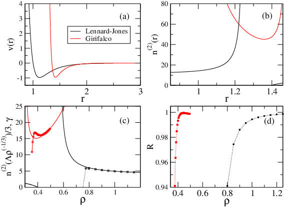
To confirm the relation between the sign of and that of and exhibit the relation between adiabats and contours we carried out simulations on two model systems. Figure 3(a) shows the pair potentials. Note that the Girifalco potential diverges at ; this hard core restricts the density to be somewhat smaller than for the LJ case, if a non-viscous liquid is to be considered. Part (b) shows the effective exponent . There is a singularity where the second derivative vanishes (the transition from concave up to concave down), which can be seen in the figure at for LJ and for Girifalco; as decreases from the singularity decreases monotonically in the LJ case, while in the Girifalco case it first decreases and then has a minimum before increasing and in fact diverging as is approached. Part (c) of the figure shows the estimate of from Eq. (31) along with calculated in simulations along an adiabat for each system. Here was determined by matching with at the highest density. The agreement is good for not too low densities—as mentioned above when diverges due to the curvature of the potential vanishing, then both and will rapidly approach zero, which is what we can see happening for the Girifalco system in parts (c) and (d) and low density. Note that the adiabat for the Girifalco system rapidly reaches rather high temperatures, since the exponent is always greater than 15, or roughly three times that of the LJ system. More interestingly, for the Girifalco system changes sign at a density around 0.4, so we can expect the dependence of along an adiabat to reflect this. The location and value of the minimum in do not match those for , however—perhaps the vanishing of the curvature is already having an effect.


The procedure for determining adiabats is described in Appendix C. Figures 4 and 5 show along adiabats for the LJ and Girifalco systems, respectively. For the LJ case the slope is positive, which is consistent with being negative as discussed in Section III. It is worth noting that the overall variation of is quite small, of order 0.1 per particle for the density range shown, but it is not negligible, even though the system has strongly correlations and the structure and dynamics have been shown to be quite invariant along the adiabats. For the Girifalco system the slope is positive at low density until a maximum is reached, with a negative slope at higher densities. This is also broadly consistent with the expectations from Fig. 3 (the locations of the maxima are not expected to be accurately given by Eq. (31)).
III.4 Contours of and directly compared


As an alternative to considering how varies along an adiabat, we can find the contours of separately. First we simulated several isochores, then the data were interpolated to allow constant- curves to be constructed. Specifically, we find that the dependence of on temperature along an isochore can be accurately fitted by the expression
| (40) |
where , and are functions of . This expression was inspired by the Rosenfeld-Tarazona expression for the specific heat;[43] we do not constraint the exponent to be 2/5, however. The expression can easily be inverted to yield the temperature corresponding to a given value of , as a function of density
| (41) |
The contours are shown along with the adiabats in Figs. 6 and 7. Recall that in typical liquids we expect to increase as decreases or increases. For the LJ case the contours have a higher slope than the adiabats, therefore as increases along an adiabat we cross contours corresponding to higher values of . For the Girifalco system the contours have initially (at low density) higher slopes than the adiabats but then bend over and have lower slopes. Thus the picture is consistent with the data for along adiabats shown in Figs. 4 and 5. It cannot be otherwise, but there is more information here compared to those figures. For example the adiabats are closer to the straight lines (in the double-log representation) expected for IPL systems, while the -contours have more non-trivial shapes. Furthermore a small variation of along an adiabat could hide a relatively large difference in slope between -contours and adiabats (since is typically a relatively slowly varying function).
IV Fluctuation formula for generating contours of
Apart from investigating the variation of along an adiabat, it is of interest to identify the contours of ; the non-constancy of along an adiabat is equivalent to the statement that the contours do not coincide with the adiabats, although we can expect them to be close for Roskilde liquids. In practice we identify contours using the interpolation procedure described above, but it is potentially useful from a theoretical point of view to have a fluctuation formula for the slope of these curves. This we derive in this section.
Since the variation of along an adiabat (Eq. 22) involves the difference between two triple correlations (which vanishes for perfect correlation); it is tempting to speculate that the ratio
| (42) |
which equals for perfect correlation, gives the slope of curves of constant . In fact, it is not quite so simple. The total derivative of with respect to along an arbitrary slope in the , plane is
| (43) |
We need to calculate the partial derivatives with respect to and . From appendix D:
| (45) | ||||
| (46) | ||||
| (47) |
Inserting this into Eq. (44) gives
| (48) |
It might seem surprising that the third moment appears, since one expects the limit of large that the distribution converges to a Gaussian, in accordance with the central limit theorem. A closer look at the proof of that theorem shows that when considering the summed variable (here the total potential energy), all the so-called cumulants are proportional to , and both the second and third moments are equal to the corresponding cumulants, and therefore proportional to . It is when one considers the average instead of the sum (potential energy per particle instead of total potential energy) that one finds the third moment and cumulant vanishing faster than the second ( as opposed to ) in the limit of large .
The density derivative of
| (49) |
is evaluated in Appendix D with the result
| (50) |
The derivative of along an arbitrary slope is then
| (51) |
Note that with we recover Eq. (22). When the correlation is not perfect we can set this expression to zero and solve for the slope which gives curves of constant , now calling it :
| (52) |
or
| (53) |
Again we check the case of perfect correlation where we can replace by and see that we get as we should. We can also write this as plus a correction term:
| (54) |


Figure 8 shows the fluctuation-determined slope of a contour in the -plane along the contour of the LJ system. We present the -contour here to be able to check the validity of the exponent: The (fixed) exponent determined by a fit of the contour to a power law is also indicated for comparison. A clear trend is observed with higher than , and like the latter decreasing towards 4 as the density increases. There is some scatter due to the difficulty in determining third moments (compare the data for which are based on second moments), so this would not be a practical method for determining the contours. On the other hand, if we are interested in knowing roughly how big the difference in slope between an adiabat and a -contour is, we do not need to simulate a -contour–we can simulate a few state points, perhaps on an isochore, and estimate the from fluctuations. The scatter is not a big problem if we are not using to determine where to simulate next. Fig. 9 compares with for both LJ and Girifalco system along an adiabat, and the trends are very clear: the -contours have definitely larger slope for the LJ system, closer to 6 than 5 (they must converge to 4 at high density). For the Girifalco system the differences are quite dramatic, more so than the direct comparison of the contours in Fig. 7 (where a logarithmic temperature scale was used). It is worth noting that all the data here correspond to state points with , i.e., very strong correlation, and that nothing special happens when the exponents are equal (e.g. in Fig. 9(b)) (in any system one can define phase-space curves along which ; it would be significant only if a two-dimensional region of equality existed).
V Discussion
V.1 Roskilde liquids are more than, and more interesting than, IPL liquids
IPL liquids are perfectly correlating and have perfect isomorphs—straight lines in the plane with slope given by one third of the IPL exponent. In this case the phase diagram is completely degenerate—the isomorphs are contours of excess entropy, and all structural and dynamical properties (when expressed in reduced units). Liquids which have strong, but not perfect correlation are much more interesting: we can still identify excellent isomorphs via Eq. (5), as adiabats, but these are no longer constrained to be power laws; the effective exponent can vary along an isomorph/adiabat and can exhibit non-trivial density dependence.[41] Moreover contours deviate now from the isomorphs/adiabats in a manner connected to the density dependence of .
It is interesting to compare the insight obtained from statistical mechanical versus thermodynamic considerations. Using statistical mechanics —the arguments leading to Eq. (38)—we have shown that vanishes when correlation is perfect, and this occurs only for (extended) IPL systems (see Eq. 30). We have also argued that in liquids with strong but not perfect correlations the temperature derivative is relatively small, therefore as a first approximation it can be ignored, leaving the density dependence of as a new characteristic for a Roskilde liquid. On the other hand the purely thermodynamic arguments presented in Ref. 32 constrain only to be zero, leaving free to depend on density, which allows for the richer set of behaviors just mentioned. The thermodynamic argument leads more directly (and elegantly) to the empirical truth—that in practice ’s temperature dependence is small compared to its density dependence—while the statistical mechanical arguments fill in the details of why this is the case.
V.2 Status of and relation between different derivatives
The claim (38) needs to be thoroughly investigated by simulation for a wider range of systems as does the validity of Eq. (31) as an estimate of . While we have argued these for high temperatures and densities, their validity could turn out to depend on how strong -correlation a liquid has, though it seems that is not necessarily required, that is, they apply more generally than strong correlation. One could imagine that it would be useful to derive a fluctuation formula for . We have indeed derived such a formula, see Appendix E, but it is not particularly simple, and we have not been able to use it to make a more rigorous theoretical connection with —even the sign is far from obvious due to near cancellation of the various terms. Its usefulness in simulations is also expected to be limited since it involves fluctuations of the so-called hypervirial (the quantity used to determine the bulk modulus from fluctuations[44]) which is not typically available in an MD simulation. On the other hand, given our results, one can use the quantity or the formula for to determine the sign of from a simulation of a single state point.
V.3 Adiabats versus contours in non-Roskilde-simple liquids

It is interesting to consider a non-simple liquid, where there is no reason to expect that -contours at all coincide with adiabats (i.e. there are not good isomorphs). We have done so for two liquids without actually determining the -contours; instead we just calculated the exponent from the fluctuations. As mentioned above this is accurate enough to give an idea of the trends, in particular which way the -contours are oriented with respect to the adiabats. The first example is the Dzugutov fluid.[36] Fig. 10 shows and for this system along an adiabat. In the range shown takes values from to . As the figure shows is substantially smaller than . We can note also that this is consistent with the positive slope , and suggests the arguments leading to Eq. (38) do not necessarily require strong correlation. Another example is the Gaussian core potential,[14] for which data is also shown in Fig. 10. In this case there is almost no correlation; , and in fact and even have opposite sign (although both are close to zero). Moreover this system clearly violates Eq. (38), since decreases with density on the adiabat shown, which should correspond to the case (as in the LJ case); this is not surprising since it does not have a hard core.
V.4 Relevance of adiabats versus contours

In our simulation studies of isomorphs, the procedure has always been to use Eq. (5) to generate adiabats (straightforward, since an accurate estimate of is readily computed from the fluctuations) and then examine to what extent the other isomorph-invariant quantities are actually invariant along these curves. One could also generate contours and check for invariance along them. While it is not obvious that adiabats are more fundamental, Rosenfeld has proposed that transport properties are in fact governed by the excess entropy.[45] Given the not insignificant difference between adiabats and -contours it is worth checking explicitly whether measures of dynamics are more invariant along one versus the other. This is done in Fig. 11 for the reduced diffusivity . It is clear that by the this measure, the dynamics are more invariant along adiabats than along -contours, consistent with Rosenfeld’s theory. We note also that the adiabats seem to be simpler than the -contours in that the exponent varies less than the exponent . This is true for the all the systems presented here including simple and non-simple ones. This implies is more practical as a liquid characteristic than and suggests that adiabats provide a more useful, and fundamental basis for describing the phase diagram than -contours. In fact a phase diagram would be consistent with the traditional starting point of statistical mechanics—a function expressing the dependence of internal energy on entropy and volume (though typically the total entropy, not , is considered).
VI Conclusion
We have derived several exact results relating to Roskilde-simple liquids (previously termed strongly correlating liquids) in the form of fluctuation formulas for various thermodynamic derivatives. These include the derivative (with respect to ) of an arbitrary NVT averaged dynamical variable along a configurational adiabat, Eq. (17), the derivative of along an adiabat, Eq. (22), the temperature derivative of itself on an isochore, Eq. (27), and the slope of contours of in the plane, Eq. (53). In addition to the exact formulas we have argued that when is negative (positive) one expects that is positive (negative) and that the slopes of -contours are greater (less) than those of adiabats. This we have tested with two model Roskilde-simple liquids, the Lennard-Jones fluid with and the Girifalco potential which has at low density but switches to at high density. From this argument emerged a claim, Eq. (38) equating the sign of the temperature derivative of to the density derivative along an adiabat for a wide class of liquids (wider than Roskilde-simple liquids). Finally we note that the data presented here provide support for the use of the exponent, determined purely by the pair potential, as a quick and convenient way to estimate and its density dependence.
Appendix A Derivation of Eq. (13)
As in appendix A of Ref. 18, we use a discrete-state notation for convenience, such that is the value of observable in microstate and the (configurational) partition function is . We have
| (55) | ||||
| (56) | ||||
| (57) | ||||
| (58) |
In the second last step the definition of the virial for a micro-configuration, was used; the density derivative is understood to mean that the reduced coordinates are held fixed while the volume is changed.
Appendix B Derivation of Eq. (22)
Here we give the details of the derivation of the expression for the derivative of at constant . Writing the variance of as allows us to use Eq. (17) to take the derivative of and Eq. (18) to differentiate .
| (59) | ||||
| (60) | ||||
| (61) | ||||
| (62) |
where we have used Eqs. (3) to write the covariance in terms of the variance of . Inserting this result with Eq. (21) gives the relatively simple formula
| (63) |
We make one more change by writing , so that
Appendix C Generating configurational adiabats
Eq. (5) indicates a general procedure for generating adiabats: (1) evaluate from the fluctuations at the current state point; (2) choose a small change in density, say of order 1% or less; (3) use Eq. (5) to determine the corresponding change in temperature:
| (67) | ||||
| (68) |
We have used this method for the Girifalco system with for values of between 0.4 and 0.5. For generalized Lennard-Jones systems there is now an analytic expression for the -dependence of which allows large changes in , the so-called “long jump method”:[32, 33]
| (69) | ||||
| (70) |
where the energy/temperature scaling function is defined by (see Refs. 32, 33; the normalization is such that ).
| (71) |
Here is a parameter which according to the theory of isomorph---i.e., assuming perfect isomorphs for LJ systems---is a constant. More generally one may expect that it is fixed for a given isomorph, but can vary weakly among isomorphs, analogous33 3 There is in fact a close connection between and ; by identifying Eq. 31 with the logarithmic derivative of we find that can be expressed in terms of the curvature of the pair potential, and moreover it becomes clear how to include dependence on in . This connection will be discussed in more detail elsewhere.[41] to in Eq. (31). It can be evaluated at a given density via (since [32])
| (72) |
(at this becomes simply ). Since the theory is not exact, and determined this way will also vary weakly along the isomorph, in order to get the best determination of the adiabats we re-evaluate at each state point. It therefore also has an index . We observe a systematic variation in of at most 0.5% for a given adiabat, and a few percent variation between adiabats. We have used the long-jump formula for the LJ system with for values of between 0.8 and 1.4. We noticed more noise in the data for the Girifalco system, but have not checked whether this is due to not having a long-jump formula or to differences in effective sampling rate (because of different relaxation times) giving different statistical errors.
Appendix D Derivation of exponent
The temperature derivative of , Eq. (44), is obtained as follows:
| (78) | ||||
| (79) |
For the density derivative of we have likewise
| (80) |
Starting with the second term, using Eq. (13)
| (82) | ||||
| (83) |
Combining the two terms then gives
| (84) | ||||
| (85) |
which is Eq. (50). Now we can assemble the derivative of along an arbitrary slope (Eq. (43)):
| (86) | ||||
| (87) |
which can be rewritten as Eq. (51).
Appendix E Fluctuation formula for the derivative of
We include here, omitting the derivation, the fluctuation formula for the derivative of with respect to at constant . The quantity is the hypervirial, which appears in fluctuation expressions for the bulk modulus.[44]
| (88) |
For IPL systems we have and , so that the derivative is zero.
Acknowledgements.
The centre for viscous liquid dynamics “Glass and Time” is sponsored by the Danish National Research Foundation’s grant DNRF61.References
- [1] I. Z. Fisher, Statistical theory of liquids (University of Chicago, Chicago, 1964).
- [2] S. A. Rice and P. Gray, The statistical mechanics of simple liquids (Interscience, New York, 1965).
- [3] H. N. V. Temperley, J. S. Rowlinson, and G. S. Rushbrooke, Physics of simple liquids (Wiley, 1968).
- [4] N. K. Ailawadi, Phys. Rep. 57, 241 (1980).
- [5] J. S. Rowlinson and B. Widom, Molecular theory of capillarity (Clarendon, Oxford, 1982).
- [6] C. G. Gray and K. E. Gubbins, Theory of molecular fluids (Oxford University Press, 1984).
- [7] D. Chandler, Introduction to modern statistical mechanics (Oxford University Press, 1987).
- [8] J. L. Barrat and J. P. Hansen, Basic concepts for simple and complex liquids (Cambridge University Press, 2003).
- [9] P. G. Debenedetti, AICHE J. 51, 2391 (2005).
- [10] J. P. Hansen and I. R. McDonald, Theory of Simple Liquids (Academic Press, New York, 1986), 3rd ed.
- [11] J. F. Douglas, J. Dudowicz, and K. F. Freed, J. Chem. Phys. 127, 224901 (2007).
- [12] B. Kirchner, Phys. Rep. 440, 1 (2007).
- [13] B. Bagchi and C. Chakravarty, J. Chem. Sci. 122, 459 (2010).
- [14] F. H. Stillinger, J. Chem. Phys. 65, 3968 (1976).
- [15] M. Engel and H.-R. Trebin, Phys. Rev. Lett. 98, 225505 (2007).
- [16] V. Van Hoang and T. Odagaki, Physica B 403, 3910 (2008).
- [17] T. S. Ingebrigtsen, T. B. Schrøder, and J. C. Dyre, Phys. Rev. X 2, 011011 (2012a).
- [18] N. P. Bailey, U. R. Pedersen, N. Gnan, T. B. Schrøder, and J. C. Dyre, J. Chem. Phys. 129, 184507 (2008a).
- [19] N. P. Bailey, U. R. Pedersen, N. Gnan, T. B. Schrøder, and J. C. Dyre, J. Chem. Phys. 129, 184508 (2008b).
- [20] T. B. Schrøder, N. P. Bailey, U. R. Pedersen, N. Gnan, and J. C. Dyre, J. Chem. Phys. 131, 234503 (2009).
- [21] N. Gnan, T. B. Schrøder, U. R. Pedersen, N. P. Bailey, and J. C. Dyre, J. Chem. Phys. 131, 234504 (2009).
- [22] T. B. Schrøder, N. Gnan, U. R. Pedersen, N. P. Bailey, and J. C. Dyre, J. Chem. Phys. 134, 164505 (2011).
- [23] J. K. Johnson, J. A. Zollweg, and K. E. Gubbins, Mol. Phys. 78, 591 (1993).
- [24] E. A. Mastny and J. J. de Pablo, J. Chem. Phys. 127, 104504 (2007).
- [25] V. V. Brazhkin, Y. D. Fomin, A. G. Lyapin, V. N. Ryzhov, and K. Trachenko, JETP Lett. 95, 164 (2012a).
- [26] V. V. Brazhkin, Y. D. Fomin, A. G. Lyapin, V. N. Ryzhov, and K. Trachenko, Phys. Rev. E 85, 031203 (2012b).
- [27] V. V. Brazhkin, Y. D. Fomin, A. G. Lyapin, V. N. Ryzhov, E. N. Tsiok, and K. Trachenko (2013), eprint 1305.3806.
- [28] U. R. Pedersen, N. Gnan, N. P. Bailey, T. B. Schrøder, and J. C. Dyre, J. Non-Cryst Solids 357, 320 (2011).
- [29] A. A. Veldhorst, L. Bøhling, J. C. Dyre, and T. B. Schrøder, Eur. Phys. J. B 85, 21 (2013).
- [30] T. S. Ingebrigtsen, T. B. Schrøder, and J. C. Dyre, J. Phys. Chem. B 116, 1018 (2012b).
- [31] N. Gnan, C. Maggi, T. B. Schrøder, and J. C. Dyre, Phys. Rev. Lett. 104, 125902 (2010).
- [32] T. S. Ingebrigtsen, L. Bøhling, T. B. Schrøder, and J. C. Dyre, J. Chem. Phys. 136, 061102 (2012c).
- [33] L. Bøhling, T. S. Ingebrigtsen, A. Grzybowski, M. Paluch, J. C. Dyre, and T. B. Schrøder, New J. Phys. 14, 113035 (2013a), eprint arXiv:1112.1602.
- [34] D. Gundermann, U. R. Pedersen, T. Hecksher, N. P. Bailey, B. Jakobsen, T. Christensen, N. B. Olsen, T. B. Schrøder, D. Fragiadakis, R. Casalini, et al., Nature Physics 7, 816 (2011).
- [35] U. R. Pedersen, N. P. Bailey, T. B. Schrøder, and J. C. Dyre, Phys. Rev. Lett. 100, 015701 (2008).
- [36] M. Dzugutov, Phys. Rev. A 46, R2984 (1992).
- [37] L. A. Girifalco, J. Phys. Chem. 96, 858 (1992).
- [38] (2012), URL http://rumd.org.
- [39] H. Robbins and J. Van Ryzin, Introduction to statistics (Science Research Associates, 1975).
- [40] To “correlate with” means to multiply by and take an ensemble average.
- [41] L. Bøhling, N. B. Bailey, T. B. Schrøder, and J. C. Dyre (2013b), manuscript in preparation.
- [42] Our method of determining fails when is constant, but the value of where one should evaluate is in principle well-defined.
- [43] Y. Rosenfeld and P. Tarazona, Mol. Phys. 95, 141 (1998).
- [44] M. P. Allen and D. J. Tildesley, Computer Simulation of Liquids (Oxford University Press, 1987).
- [45] Y. Rosenfeld, J. Phys.: Condens. Matter 11, 5415 (1999).
- [46] There is in fact a close connection between and ; by identifying Eq. 31 with the logarithmic derivative of we find that can be expressed in terms of the curvature of the pair potential, and moreover it becomes clear how to include dependence on in . This connection will be discussed in more detail elsewhere.[41].