Multiple Higgs-Portal and Gauge-Kinetic Mixings
S. Y. Choi1, C. Englert2, and P. M. Zerwas3
1 Department of Physics, Chonbuk National University, Jeonju 561-756, Republic of Korea
2 SUPA, School of Physics and Astronomy, University of Glasgow, Glasgow, G12 8QQ, United Kingdom
3 Theory Group, Deutsches Elektronen-Synchrotron DESY, D-22603 Hamburg, Germany
(August 24, 2026)
Abstract
We develop a phenomenological formalism for mixing effects between the Standard Model and hidden-sector fields, motivated by dark matter in the Universe as well as string theories. The scheme includes multiple Higgs-portal interactions in the scalar sector as well as multiple gauge-kinetic mixings in the abelian gauge sector. While some of the mixing effects can be cast in closed form, other elements can be controlled analytically only by means of perturbative expansions in the ratio of standard scales over large hidden scales. Higgs and vector-boson masses and mixings are illustrated numerically for characteristic processes.
1 Basics
A large fraction of matter in the Universe is invisible
[1]. This hidden sector may have structures at least
as complex as matter and interactions in the visible Standard Model
[SM] sector (see e.g. [2]), unlike one-component
theories as realized in supersymmetry approaches to the dark
sector. Opportunities to explore structures in this hidden sector are
offered by mixing effects with fields of the SM. Couplings between
the two sectors are provided by Higgs-portal interactions
[3, 4, 5, 6, 7]
and gauge-kinetic mixings
[4, 8, 9]. Higgs-portal interactions couple
the invariant bilinear product of the Higgs field in the Standard
Model with Higgs SM-singlets in the hidden sector [HS], the strength
of the interaction measured by . Kinetic mixing couples abelian
hypercharge -field tensors in both sectors with strength .
The coupling can be varied in the analysis in a large range
[10], , and the kinetic coupling in the most
general scenario in a similar range , depending strongly
however on the underlying microscopic picture of the mixing
mechanism.11
1
We are very grateful to J. Jaeckel for valuable
advice on field- and string-theoretic models of kinetic mixing and
consequences for the potential range of . If in
field-theoretic models loops of mediators link the hypercharge
fields in the two sectors, the size of is expected to be
restricted to , set in detail by the gauge
couplings, the hypercharges and the masses [8]. On the
other hand, the kinetic coupling as mediated by string states is less
stringently restricted in general, and it can be quite large depending
on the type of string theory realized, see e.g. [11].
We will not delve into building a detailed model of the joined
[SM][HS] system, nor of dark-matter candidates. However, the
HS system may be taken as a SM-type system [12], properly
extended to accommodate the dark-matter properties. The lightest
fermion field, among others, could be a stable candidate in such a
scenario for the dark-matter field. The hidden-sector scales will be
assumed of TeV size, contrasting approaches in which fields are
assumed super-light. The present analysis aims at exploring the
potential of high energy colliders, LHC
and LC, for shedding light on the structure of a heavy hidden sector.
The SM electroweak gauge interaction of the -field is unaltered by
kinetic mixing to leading order and the procedure of high-precision SM
analyses is modified only to second order. Also, the Higgs-portal
interactions have been introduced in renormalizable form. As a result,
well-explored low-energy physics is not dramatically affected, and
changes are just
restricted to potentially small corrections.
It turns out that the re-diagonalization of the gauge sector after
switching on kinetic mixing is surprisingly straightforward and the
results can largely be presented in transparent analytic
form. However, the re-diagonalization of the effective mass matrix of
the gauge fields, parallel to the re-diagonalization of the mass
matrix in the Higgs sector, can in general be carried out analytically
only by expanding mass eigenvalues and field eigenvectors in the ratio
of SM masses over dark masses, the latter assumed to be large, i.e.
in the TeV regime [13].
First we will discuss both Higgs-portal mixing and gauge-kinetic
mixing quite generally. Thereafter we will turn to numerical examples
for Higgs and vector fields in a hidden sector coupled either by one or
two links to the SM, i.e. and mixing
scenarios. Specifically we will address the problem of how to encircle
parameters such that the structure of the combined system can be
tested. We will analyze the problem of how to extract, at LHC and LC,
the basic mass parameters
and the mixings between the hidden sector and the measurable SM.
1.1 Higgs Portal : Multiple Couplings
In the extended Higgs sector we will assume that the SM iso-doublet
Higgs field is complemented by a set of complex scalar
fields that generate the hidden gauge boson masses, including the
U(1) gauge bosons , which are mixed with
the hypercharge SM gauge boson. Expanding the fields about the minimum
of the scalar potential, the real SM Higgs field and
hidden-sector Higgs fields will emerge,
corresponding to scalars located primarily in the visible SM sector
and the invisible hidden sector, respectively. The two sectors are
coupled weakly and they are linked
by bi-linear quartic couplings, leaving the system renormalizable.
Cast into the standard formalism of spontaneous symmetry breaking, the Higgs potential is introduced as
| (1) |
The parameters are negative, shifting the ground states to
non-zero vacuum values, and the parameters are positive to
stabilize the system. As we focus primarily on the direct coupling of
the SM Higgs field and the hidden-sector Higgs fields, quartic
interactions among the hidden-sector Higgs fields can be ignored to
leading order in this context if the couplings of the mixing terms are
taken to be small. Their impact on any physical observables will be
suppressed when passing the Higgs-portal. [For illustration, the
analysis including small quartic mixing
in the hidden sector is summarized in Appendix A.
Introducing the vacuum Higgs values at the minimum of the potential,
| (2) |
where is the neutral component of the SM iso-doublet Higgs field etc, they can be expressed by the potential parameters after solving the minimum conditions:
| (3) | |||||
| (4) |
Inserting mutually into and v.v., the set of two equations
has been solved for and supplementing the original values
of the individual sectors, and
, before they are coupled by
.
The bilinear kinetic terms and the mass terms of the physical Higgs fields are described by the effective Lagrangian:
| (5) |
The parameter denotes the mass of the SM Higgs boson in the current basis, the matrix denotes the mass matrix of the Higgs bosons in the hidden sector [for simplicity assumed to be diagonal], and the -dimensional column vector accounts for the couplings of the scalars in the SM and the hidden sectors:
| (6) | |||||
| (7) | |||||
| (8) |
expressed by the basic parameters of the potential. [In the general
case with quartic terms of hidden-sector Higgs fields, the matrix
is non-diagonal but symmetric so that it can be diagonalized
by an orthogonal transformation. The mixing vector is changed
slightly as a result, see Appendix A.]
The mass matrix in the current representation will be transformed to the diagonal mass matrix in the mass representation by applying the orthogonal transformation :
| (9) |
while the Higgs fields transform as
| (10) |
For and higher, the eigenvalues and eigenfunctions of the mass matrix cannot be written in closed or transparent form anymore. But they can be expanded consistently for small mixing up to second order in the expansion parameter [13]:
| (11) | |||||
| (12) |
while the orthogonal transformation matrix up to second order reads
The corrections of the heavy hidden Higgs masses are in general
not diagonal. However, re-diagonalization gives rise to changes of the
eigenvalues and mixing matrices only beyond the order considered so
that the off-diagonal elements can simply be truncated [see the proof
in the Appendix].
By assuming the mass parameters in the hidden sector to be heavy compared with the SM sector and the mixing parameters, the norm of the vector is small and serves as an expansion parameter, in parallel with . The SM Higgs mass parameter however could be modified sizably if the mixing parameter is not much smaller than the SM parameter [consistent with the expansion]. To lowest order, the modifications of the masses and the mixing matrix,
| (16) | |||||
| (17) |
mcc and
| (18) |
are particularly simple. This set of transformations of the
wave-functions generates the reduced couplings of the SM-type Higgs boson
and the couplings of the hidden Higgs bosons
with the SM gauge and matter fields to first order in the mixing.
In the Higgs scenario the solution can be reconstructed
analytically without any expansion [10, 14]. The
mixing matrix is the standard 22 matrix built up by
and of the rotation angle . After reducing the vector
to the small mixing angle , the above
relations are readily recovered from the system, as
will be recalled later.
Starting from the lowest order, masses and mixings can iteratively be
constructed to arbitrary order in the expansion parameter
, both of
which are small for large masses in the hidden sector, compared to
SM masses and mixings. The perturbative recursion formulae are derived
in the Appendix.
1.2 Kinetic Mixing
The interaction between the SM hypercharge -field and the set of gauge fields concentrated in the hidden sector, is described by the Lagrangian
where is the current gauge-boson mass matrix given by
in terms of the mass parameter ,
the sine/cosine of the electroweak mixing angle
etc, as well as the dimensionless matrix ,
after including the mixing of the SM neutral iso-spin -field and
the hypercharge -field due to electroweak symmetry breaking. While
the field vectors are denoted by , the field
tensors are denoted by ; is the -dimensional vector accounting for the kinetic
- mixings. For the sake of notational simplicity we have
refrained from introducing mixing among the fields in the hidden
sector, which can easily be added .
Applying an matrix transformation, consisting of a kinetic transformation [KT] and a rotation, to the gauge fields, the kinetic mixing of the field strengths can be absorbed in the redefinition of the fields. Thereafter, the mass matrix must be diagonalized by a matrix split into the block-diagonalization matrix and the rotation matrix re-diagonalizing the mass submatrix in the hidden sector. The block-diagonalization can be performed only approximately; the expansion parameters being and , with the norms assumed to be small. The final result of this procedure can be written as follows:
| (39) |
leading to the massless photon field , and the massive vector fields and . The KT matrix and the block- and re-diagonalization matrices read
with the -dimensional column vector
| (50) |
to lowest order in the mixing. [ actually proves
ineffective
to lowest order, as derived in the Appendix.]
The submatrix in is a symmetric matrix defined by the dyadic product of the mixing parameters ,
| (51) |
which can be diagonalized by the orthogonal matrix ,
generating the diagonal matrix . The set of eigenvalues of
the dyadic matrix consists of one non-zero value
followed by zero values, giving rise to the diagonal
matrix .
The spectrum and the eigenvectors are derived in the Appendix.
Switching from the current basis to the mass basis, the mass matrix is transformed, up to second order, to the diagonal mass matrix in Eq. (39), representing the zero photon mass and the non-zero mass eigenvalues up to second order as
| (52) | |||||
| (53) | |||||
| (54) |
where diagonalizes the matrix up to the second-order
approximation of the mixing.
Special attention should be payed to the peripheral null-vector in the matrix . This form is essential to keep the SM gauge interactions intact to leading order. This is apparent by noting the covariant derivative which transform as
| (55) | |||||
with and up to linear approximation
in the kinetic mixing; as usual, , and . The coefficients of the and fields are not
altered preserving the standard structures in the original
electroweak sector after electroweak symmetry breaking at this level.
2 Analysis
The simplest example of portal models combines the SM with just one
new degree of freedom in the hidden sector. With some elements
worked out already a while ago, cf. Ref. [3], we extend
the analysis in this section at the level of phenomenology as well as
analytical solutions based on perturbative expansions. Note that the
Higgs and the gauge sectors are entangled, the connecting link being
the transformed vacuum expectation values of the Higgs fields affecting
the current mass parameters of the gauge fields.
2.1 Higgs system
Specifying the notation in the previous sections, the physical Higgs masses and the Higgs mixing angle , derived from the current Higgs mass matrix,
are given by
| (59) | |||
| (60) | |||
| (61) |
up to the second order approximation in for the masses. It should be noted that the leading mass corrections are not suppressed by the large hidden scale , in contrast to the mixing angle. The current Higgs fields and the mass Higgs fields are related by the orthogonal transformation :
where can be assumed non-negative without loss of generality. These three observables can be exploited, in return, to extract the individual vacuum parameters and according to
| (69) | |||||
| (70) | |||||
| (71) |
While the measurement of the two Higgs masses, and , is self-evident, the mixing parameter can be determined from the Higgs-gauge boson vertex, i.e.
| (72) |
where is given by the mass
| (73) |
with the SU(2)L gauge coupling derived from the measured
-width in a model-independent way to leading order.
[The hypercharge coupling is derived correspondingly from combining
the electron electromagnetic-magnetic coupling and with the
hypercharge relation .]
The quartic couplings , or equivalently the vacuum expectation values , can be separated only by measuring the triple Higgs couplings. Denoting the current triple Higgs couplings by , they can be expressed by the physical couplings in the mass basis as
| (74) |
The tensor components can be written as
| (75) | |||||
| (76) | |||||
| (77) | |||||
| (78) |
with the abbreviations etc; they are symmetric under
index permutations. The Feynman rules follow from multiplying the
above equations by a minus sign and a combinatorial factor that counts
the number of the identical external legs. The parameter of the
hidden sector is naturally associated either with [small] mixing
coefficients or with coupling/mass suppressed degrees of
freedom.
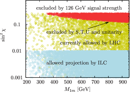
For illustration purposes, we pick, with GeV, a representative parameter point
| (79) |
from the scan of the allowed points depicted in
Fig. 1 [choosing a SM-like width of ].
Identifying the mass of with 125 GeV, the global area of the
two unknown parameters, i.e. the second Higgs mass and the
mixing , is tightly constrained by future precision
measurements of the boson. For a numerical investigation of
the above parameter point we adopt the extrapolations to
for LHC at 14 TeV and adopt an energy of 250 GeV
for ILC as provided in Ref. [16]. A measurement of
and the masses and , which will be well
established at the quoted LHC luminosity, is not enough to separate
vacuum expectation values from quartic couplings in the most general
and complete analysis of the system. We need (at least)
one additional measurement in order to reconstruct all the
parameters individually.
There are two independent approaches to this problem, depending on the
size of the invisible Higgs branching ratios. For large values, we can
use an invisible Higgs measurement to constrain the parameter
as described in Ref. [10].
Since recent measurements of point towards a SM-like total
width (at least when SU(2)L doublets are
involved [17]) we investigate a different
possibility in the following, assuming no direct partial decay width
of to the hidden sector. Then phenomenology is dominated by
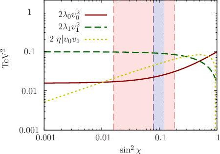
mixing only and we can use an experimentally measured region of
to constrain the system of mass relations in
Eqs. (69), (70) and
(71) as shown in Fig. 2. The
additional information to reconstruct the individual parameters should
then be made available from the measurement of the trilinear Higgs
couplings in Eqs. (75)-(78)
[10, 18], which can be phenomenologically accessed via
light dihiggs production, i.e. predominantly at
the LHC [19]. [Recall that in scenarios
is known from the mass and the SU(2)L gauge coupling
measured by the width, both of which are not affected by U(1)
mixings.]
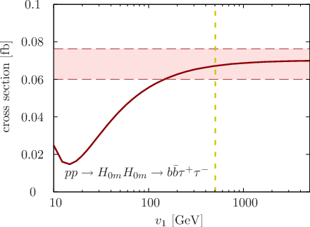
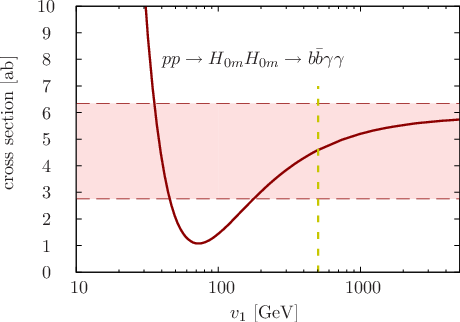
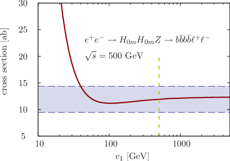
Recent analyses [20] indicate that a
variation of the trilinear Higgs coupling is only feasible in the
context of the SM in the channel
[21] if possible at all. Rare Higgs decays such as
[22] are clean
[ for 12 signal events in
[20].] Nevertheless the involved
uncertainties are too large and the signal yield is too small to
obtain a more fine grained picture. In contrast to the SM, however,
the scenario offers the possibility to discriminate the
signal region from the “continuum”
production. Upon correlating the two regions we can
constrain in different channels: Electroweak precision
measurements, even for rather small mixing angles , indicate that the mass splitting between the 125 GeV boson and
must not be too large. Observing a cascade decay therefore implies small boosts of the bosons
and the analysis of the final
state is not applicable anymore. On the other hand, is inclusive in this sense and we can extract a
limit on in this channel when selecting invariant masses
. The complimentary phase space region
can again be tackled in the boosted selection using the methods of
Ref. [21].
In both analyses interference plays an important role. We therefore
use a complete leading order calculation keeping the full top mass
dependence following Ref. [18]. The result for the
two signal regions including the expected measured interval
at 14 TeV and is shown in
Figs. 3b and 3b. The dip structure
of Fig. 3b highlights the importance of the
interference effects: for
the resonant production has a global minimum due to the vanishing of
. For values the diagrams interfere destructively with the box contributions, but the grows quickly to
outrun the suppression. For the away-from-resonance region this
interference is always destructive, i.e. the smaller the larger
and the smaller the resulting cross
section until the trilinear coupling compensates the
enhanced destructive interference of with the box
contribution and the propagator suppression for very small values of
. In this sense “leaks” into the measurement
region and must not be discarded
in the actual analysis.
The region of large values is determined by the
pieces of and and the asymptotic cross section
settles at a smaller cross section with respect to the SM, mostly as a
consequence of the suppression. By contrast, given the
small mixing and the kinematic suppression, it is impossible to
observe and at the LHC [18].
Depending on the scenario, systematics etc., either the peak or the continuum analysis can perform better. In any case, both analyses can be used for cross checks and for lifting the degeneracy, if present, of the peak analysis. Using the currently known results we find a lower limit of
| (80) |
with the analysis to be compared with the
slightly larger bound for the chosen parameter point. This interval
can be mapped onto the allowed region of Fig. 2
constraining . However, as can be seen from
Figs. 3b and 3b, the
model-independent separation of the parameters and the
vacuum expectation value is in general not feasible for the
planned luminosities at LHC as an upper bound on is very loose
if it can be established at all. Even at an collider running
at GeV (Fig. 4) we can only extract a
lower limit on at an integrated luminosity of
[see Ref. [23] for a general discussion of measuring
the trilinear Higgs coupling at a linear collider]. However, given
that at this luminosity the uncertainties are still statistics-driven,
there might be the possibility to extract an upper limit on in
the far future. In fact, the quoted uncertainty band is entirely
dominated by the statistical uncertainty of the signal counts as the
search is
essentially background-free [24].
However, in theoretical scenarios which predict the values of the gauge coupling and the hypercharge in the hidden sector, the vacuum expectation value can be determined from the two vector-boson masses:
| (81) |
Thus, the fundamental current parameters in the Higgs potential can, in principle, be
extracted from experimental data, the combinations easily extracted from masses and
mixings, and the s separately bounded from trilinear Higgs
couplings or derived from vector-mass measurements in specified
theories. When the gauge couplings and charges are predicted
theoretically, all the fundamental Higgs parameters can be
extracted.
2.2 Kinetic Mixing
Analogously, the mixing of the gauge sector can be worked out explicitly. The kinetic term and the mass term are diagonalized by a kinetic transformation and an orthogonal rotation matrix as
with . The masses, in the current basis,
| (95) | |||||
| (96) | |||||
| (97) | |||||
| (98) |
are defined by the gauge couplings, the vacuum expectation values, and the SU(2) and the U(1) charges of the Higgs fields. Since the charged -field does not mix with the vector field in the hidden sector, the measured values of the -mass and width determine the parameters and and the SM relations and define , , and before mixing. The [neutral] current masses are transformed to the vanishing photon mass and two physical non-zero gauge boson masses by the rotation angle . The exact and the approximate forms, expanded up to second order in and , may be denoted as
| (99) | |||||
| (100) | |||||
| (101) |
with .
The vertices relevant for measuring the parameters of the theory, are
collected in Tab. 1.
| vertex | type | exact | expansion in mixing |
|---|---|---|---|
| 3-gauge bosons | |||
| gauge boson - fermion | |||
| Higgs - gauge boson | |||
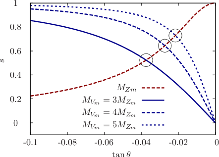
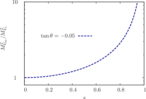
The direct measurement of the mass parameters [see e.g. Refs. [25, 26] for searches as performed by ATLAS and CMS] in the mass basis together with the indirect determination of the mass parameters in the current basis in Eqs. (99), (100) and (101) allows for a complete analysis of the fundamental vector parameters, including the KT parameter and the rotation angle . From the two relations
| (102) | |||||
| (103) |
the mixing parameters, and can be extracted, Fig. 5b. [Note that due to pure U(1) mixing the weak couplings and are fixed and measurable quantities, as outlined above, and is known.] These values can be exploited to derive the third mass parameter in the current basis:
| (104) | |||||
cf. Fig. 5b. These results can be cross-checked for
internal consistency by experimentally analyzing vertices collected in
Tab. 1. Note that oblique corrections due to kinetic
mixing are typically less important as compared to Higgs mixing since
they scale
[27]. Explicit calculation proves that they lead to
bounds which are comparable to the limits currently set by ATLAS and
CMS (see below).
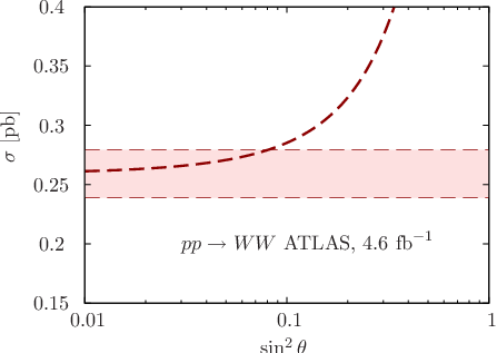
Current constraints on anomalous triple gauge boson vertices, obtained
by ATLAS [28] and CMS [29], restrict to
, Fig. 6, which becomes comparable to the
LEP combination [30]. The analysis is highly
sensitive to modifications denoted in Tab. 1, in light of
a tree-level radiation zero in the SM [31]. There
exists a completely destructive interference between the radiation
diagrams and the Feynman graph involving the vertex in the
SM. Any (non-global) deviation from the SM-predicted coupling pattern
destroys this characteristic angular dip structure resulting in an
increase of the total cross section.22
2
This is strictly true at
tree level. Gluon induced channels of the higher order-corrected
cross section lift the radiation zero. Therefore, the integrated
cross section [supplemented by a jet veto in the actual analysis] is
very sensitive to the suppression of the coupling, which can
be used to extract an upper limit on even if the
is too heavy to be measured directly.
Note that the coupling is not affected by gauge-kinetic
mixing so that it can be used to measure individually.
Subsequently, the measurement of the vertex can in
principle be used to measure the allowed range of the shift of
Tab. 1. Some concrete models of U(1) mixing in the field
and string theories [9, 4] predict the mixing
parameter to be , but string models in general allow
for rather large values well in the sensitivity range of LHC (and
ILC). A hierarchy then results in modification of the
couplings dominated by the Higgs mixing. This leaves
Drell-Yan–like production of as probably the best search
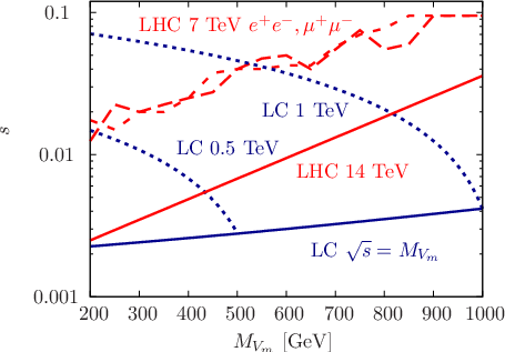
strategy in the mass region that can be covered by the LHC and future
colliders, Fig. 7. Once the vector-boson mass range
is known from LHC, LC scans can improve the sensitivity to
measurements of the kinetic mixing parameter .
3 ANALYSIS
To exemplify the analytic and numerical analyses of the preceding
sections further, we shall discuss next a more complicated system
where the SM Higgs sector is connected by portal interactions with two
Higgs systems in the hidden sector, and the U(1) hypercharge field
is mixed kinematically with two abelian U(1) fields in the
hidden sector with charges . Such a system may be
generated quite easily in superstring theories.
The microscopic parameters in the Higgs sector are chosen such that
physical masses are centered around 125, 300, 1000 GeV before mixing.
For illustration purposes we take these mass parameters to derive
for quartic Higgs-coupling values
and set , such that
is the only free parameter left. The mass associated
with the Standard Model is fixed at , the
gauge masses in the hidden sector are chosen as 300 and 1000 GeV. The
kinetic mixing vector in the gauge sector, defined as , is varied by running from 0 to 1, with
kept fixed. This choice of free parameters is
chosen minimal for the sake of transparency.
3.1 Higgs system
Reading off the bilinear mass terms from the Higgs-portal Lagrangian, the Higgs mass matrix turns out to be
This matrix could in principle be diagonalized
analytically, but the result is not transparent anymore. In the case
of small mixing the approximate results of the previous section can be
applied. In general, however, numerical methods will be adopted and
the results will be illustrated in figures.
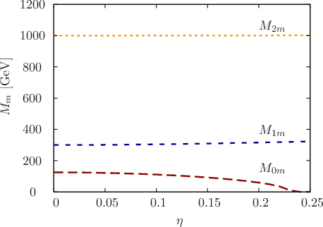
The three eigenvalues of the mass matrix are displayed in Fig. 7b for the fixed parameters as defined earlier, but the mixing parameter parameterizing the value of is varied. For small mixing, and large scales of the hidden sector, the masses are given analytically by
| (111) | |||||
| (112) | |||||
| (113) |
in second order approximation of the mixing.
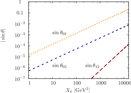
The orthogonal matrix in Eq. (10) is most elegantly parameterized by the three rotation angles associated with the rotations of the planes, i.e. . The sine-functions of the angles are shown in Fig. 7b for varied mixings as defined above. For small mixing the sines of the rotation angles read
| (114) | |||||
| (115) | |||||
| (116) |
up to linear order in the mixing.
Given the parameters, masses and mixings, of the physical states,
the production cross sections and the decay branching ratios can be
predicted in the standard way.
The mixing modifies the couplings of the original SM Higgs boson to the -gauge bosons and it generates the corresponding couplings to the original Higgs bosons in the hidden sector:
| (117) |
The coupling to -boson pairs is more involved if the kinetic
mixing modifies the current eigenstates to mass eigenstates
as discussed later.
In the same way as above, the triple Higgs couplings in the potential can be derived from the triple Higgs couplings of the mass eigenfields which are accessible, in principle, from experimental data of multiple Higgs production cross sections; in self-explaining notation for small mixing:
| (118) | |||||
| (119) | |||||
| (120) | |||||
| (121) | |||||
| (122) | |||||
| (123) |
symmetric under permutations of the Higgs indices.
Thus, three Higgs masses, the couplings of the Higgs bosons to SM pairs
and the triple Higgs couplings allow the determination of the current
parameters in the Higgs potential.
3.2 Kinetic Mixing
The mixing in the gauge sector can be illustrated in a similar
fashion. Disregarding potential mixing of the two abelian gauge fields
within the hidden sector [which could be implemented with no
problem], the kinetic mixing of the hypercharge -field with the
abelian gauge fields, and its weak mixing with the neutral SU(2)
-field, affect masses and couplings of the mass vector-eigenstates.
The KT matrix introduced in Eq. (51) is diagonalized by the orthogonal matrix
| (124) |
with for . The KT matrix turns into a diagonal matrix with . The matrix, transforming the current gauge vector fields to the mass vector fields is given by
up to the second order of the mixing , with the abbreviations
, etc. The matrix affects the
vector-boson masses and the charges when varying the KT factor
and the angle in the mixing column vector .
For a small mixing parameter , the three massive gauge boson masses, in addition to a vanishing photon mass , are given approximately by
| (134) | |||||
| (135) | |||||
| (136) |
up to the second order in the mixing. By construction, the isospin and hypercharge are not changed a priori to leading order, while the generalized charges can be derived from the transformed covariant derivative
| (137) | |||||
| (138) | |||||
| (139) |
to leading order in the mixing.
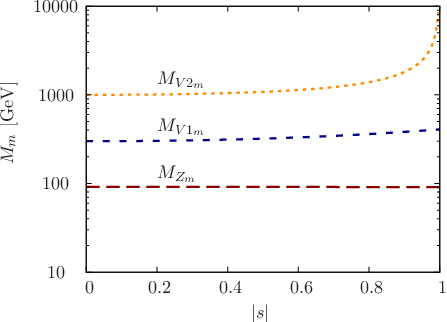
The exact mass eigenvalues of are illustrated in
Fig. 8b as a function of the kinetic mixing
parameters and . The charge components
correspondingly in Fig. 8b for couplings and .
The -dependence in these figures is easy to understand. For large
enough the mass matrix approaches the limit of
two system with only weak coupling. The masses in the hidden
sector grow for , leading to strong dependence of the
heavier hidden mass eigenvalue as a consequence of the diagonalization
of the hidden symmetric submatrix. The coefficient
approximately cancels for the lighter eigenvalue. The
cross-talk of the visible and the hidden sector gives rise to a
larger overlap of the light hidden state with the visible sector. Since
the is orthogonal to the overlap of the former state
with the visible sector becomes minimal in the limit where mixing in
the hidden sector dominates for . In this limit the coupling
of to SM matter saturates, while
decouples.
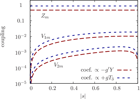
The intertwining of the SM and hidden sectors may be illustrated by noting the diagonal Higgs-vector couplings
| (140) | |||||
| (141) |
and the non-diagonal Higgs-vector couplings
| (142) | |||||
| (143) |
in which the couplings are modified only by Higgs mixing while the
and couplings are affected by the superposition of
Higgs and vector mixings.
4 Summary
In this report we have taken a first modest step in analyzing
scenarios in which the SM is coupled to a hidden sector comprising more
than one degree of freedom. The difficulty of the analysis rises
enormously with the complexity of the hidden sector that can only be
accessed through mixing effects with the SM fields. The simplest
structures of the hidden sector are abelian or [extended] SM-type gauge
theories broken by the Higgs mechanism. The Higgs fields interact with
the SM Higgs field by means of bilinear quartic couplings, the vector
fields by means of kinetic mixing with the SM hypercharge field.
In the first part we have analyzed quite generally the mixing effects
within the Higgs system and within the vector system for an arbitrary
number of degrees of freedom. Closed and transparent analytical
solutions can only be obtained for
configurations. Approximate solutions however can be obtained quite
generally to leading non-trivial order of small mixings. In the Higgs
as well as gauge sector the mass matrix can
systematically be diagonalized to arbitrary order.
Two examples illustrate the abstract analysis. For the
system we have studied a complete set of observables which allow to
reconstruct the set of fundamental parameters in the Lagrangian, in
principle. Higgs and vector-boson masses and their trilinear couplings,
supplemented by fermion couplings, generate such an ensemble. Since
all the Higgs and vector-boson states which are identified experimentally,
are mixed mass eigenstates, the effective vertices are complicated
mixtures in which Higgs mixing and kinetic mixing are intertwined. If
the mixing is too small the associated cross sections may, partly, not
be large enough to measure the vertices involved, but blocks of
essential elements
in the Lagrangian can nevertheless be isolated.
Precision analyses of the electroweak sector allow to constrain the
system at present and future colliders. Direct detection
limits at the LHC in Drell-Yan type production will give upper
production limits on the additional neutral vector boson. Other
channels like production and the search for anomalous
interactions will (and in fact already do) constrain the associated
mixing via modifying the SM coupling pattern, resulting in a
phenomenology sensitive to the described coupling modifications.
A precise measurement of the Higgs self-interaction facilitates a
complete determination of the extended Higgs-sector
parameters. Current extrapolations suggest that only a lower limit on
the hidden-sector vacuum expectation value can be established.
The potentially clean environment of a lepton collider, however,
might be able to amend this conservative statement at high
luminosity.
The study has been extended to the system in which the SM interacts
with a hidden sector comprising two Higgs and vector-boson degrees
of freedom. It could be shown that for small mixing, in addition to
the numerical evaluation, this system also can be analyzed analytically.
Furthermore, the measurement strategies that we have outlined in
Sec. 2 can be directly generalized to the analysis. The situation, however, becomes less transparent due to
the increase in parameters while the number of phenomenologically
accessible measurements [especially in the Higgs sector where large
mixing effects could be present] stays the same.
In toto. If the Standard Model is coupled weakly to a complex
hidden sector, essential elements of this novel sector can be
reconstructed, though the experimental analysis may turn out very
difficult, and partly incomplete, if mixings are too small.
APPENDIX
A Mixing in the Hidden Sector
If quartic [bi-bilinear] mixing terms in the hidden sector are included, the Higgs potential is generalized to
| (A.1) | |||||
in obvious vector/matrix notation in the second row.
The index represents the Higgs field in the SM sector, i.e. and
etc, while indices refer
to hidden-sector scalar fields.
The visible and hidden components of the vacuum Higgs fields are defined by the vanishing of the derivative of the Higgs potential,
| (A.2) | |||||
for small off-diagonal mixing parameters and diagonal parameters .
The term bilinear in the physical fields defines the masses of the Higgs particles,
Restricting the symmetric mass matrix to the components of the hidden sector in the notation of Eq. (7), the matrix can be diagonalized by an orthogonal transformation , modifying subsequently the phenomenological mixing vector in Eq. (8):
| (A.8) |
Notice that the off-diagonal mixing elements change only
to higher order so that the portal interactions between visible and hidden
sector fields are essentially not affected by the quartic mixing
in the hidden sector.
Finally, the self-interactions among the Higgs fields, SM and hidden, can be derived from the potential
| (A.9) |
in terms of the physical Higgs fields in the current [c] representation.
B Dyadic Matrix
It is straightforward to diagonalize the dyadic matrix formed by a -dimensional column vector and its transpose as
| (B.10) |
Making use of the rules for calculating determinants, one eigenvalue emerges as positive and the other eigenvalues as zero:
| (B.11) |
The eigenvectors associated with the eigenvalues read
| (B.12) |
normalized to unity.
C Block-diagonalization : Higgs and Vector Masses
1.) The eigen-masses and mixings in the Higgs sector, when block-diagonalizing the real and symmetric matrix by an orthogonal transformation ,
can iteratively be constructed from the lowest order to arbitrary
order in the expansion parameter . The first, large part of the mass matrix will be
called , the second, small part which
is order compared with . Thus, the
expansion is valid for masses in the hidden
sector large compared to SM masses and the mixings.
The conditions which determine the mixing matrix for block-diagonalization of the mass matrix are orthogonality and diagonality:
| (C.10) | |||
The first two matrices in will occasionally be
identified
with indices and 1, respectively.
(i) The orthogonality condition for determines the symmetric part of the component from as
| (C.18) |
(ii) The diagonalization condition of the mass matrix determines the antisymmetric part of from the off-diagonal block elements, and at the same time the expansion of the mass eigenvalues from the diagonal block elements:
| (C.19) |
for .
To simplify the notation we switch from indexed symbols to one-letter symbols by denoting
| (C.20) |
The matrix is taken symmetric, the antisymmetric part of is defined in the column and row. To unify the mass dimensions and express all the formulae in compact form, we introduce three dimensionless and two dimensionful matrices as
| (C.21) |
where however always come as dimensionless combinations.
The simplified recurrence relations of the matrix blocks may be cast in the following form for the block-diagonal components:
and for the off-diagonal components:
| (C.31) |
The block-diagonal components of the mass matrix are given by
| (C.35) |
2.) In the same way the mass matrix in the gauge sector can be diagonalized recursively for small gauge-kinetic mixing . After applying the KT matrix , given in closed form by
| (C.36) |
with the symmetric matrix , the transformed mass matrix
| (C.37) |
has the characteristic properties which allow the recursive diagonalization according to the algorithm developed in the previous subsection. Disregarding the photonic null-vectors, we can identify, in symbolic notation,
| (C.38) |
for the mass submatrix with
. However, the kinetic mass matrix
includes additional -dependent terms which can be expanded for
small . They add contributions to the matrix
in Eq. (C.19). Since they affect the matrix
only by already known matrices , they are easy to
incorporate. This procedure is straightforward, though technically
cumbersome, and we will not present the additional terms in detail.
D Re-diagonalization
After the block-diagonalization the mass matrix in the hidden sector is not diagonal anymore. Here, the correction
term is of the second order or higher in . It may
be re-diagonalized by the orthogonal transformation . Expanding
all the matrices, and ,
systematically in terms of the power of , the diagonal
mass matrix and the orthogonal transformation matrix can easily be
constructed recursively, as worked out before.
The orthogonality condition determines the symmetric part of in terms of the predetermined lower-order matrices by the relation
| (D.1) |
Introducing the symmetric auxiliary matrix
| (D.2) |
the diagonalization condition
| (D.3) |
can be exploited to project out the antisymmetric part of ,
| (D.4) |
with the abbreviation and the
symmetric part calculated before by means of the orthogonality
condition. The diagonalized eigenvalues are given by the elements of
the matrix in Eq. (D.2), which, at this
point, includes only predetermined matrices on the
right-hand side.
In this way the re-diagonalization of the mass matrix in the hidden sector is completed.
These solutions may be illustrated for the first three non-trivial cases. The second- and third-order terms read
| (D.5) | |||||
| (D.6) | |||||
| (D.7) |
The transformation matrix is apparently antisymmetric. As a result, the newly diagonalized mass matrix in the hidden sector is found by just truncating the mass matrix after block-diagonalization to the diagonal elements up to the third order. However, starting from the fourth order, there appear non-trivial contributions to the diagonal elements from the lower-order terms. The fourth-order terms read
| (D.8) | |||||
| (D.9) | |||||
| (D.10) |
Note that the fourth-order matrix is not antisymmetric any more.
Acknowledgements
C.E. thanks Joerg Jaeckel, Valya Khoze and Michael Spannowsky for helpful discussions. The work of S.Y.C. was supported by Basic Science Research Program through the National Research Foundation (NRF) funded by the Ministry of Education, Science and Technology (NRF-2011-0010835).
References
- [1] P. A. R. Ade et al. [Planck Collaboration], arXiv:1303.5076 [astro-ph.CO].
- [2] J. Fan, A. Katz, L. Randall and M. Reece, Phys. Rev. Lett. 110 (2013) 211302; J. Fan, A. Katz, L. Randall and M. Reece, arXiv:1303.1521 [astro-ph.CO]; M. McCullough and L. Randall, arXiv:1307.4095 [hep-ph].
- [3] R. Schabinger and J. D. Wells, Phys. Rev. D 72 (2005) 093007; B. Patt and F. Wilczek, hep-ph/0605188; M. Bowen, Y. Cui and J. D. Wells, JHEP 0703 (2007) 036; S. Chang, R. Dermisek, J. F. Gunion and N. Weiner, Ann. Rev. Nucl. Part. Sci. 58 (2008) 75; J. D. Wells, In *Kane, Gordon (ed.), Pierce, Aaron (ed.): Perspectives on LHC physics* 283-298 [arXiv:0803.1243 [hep-ph]].
- [4] E. Weihs and J. Zurita, JHEP 1202 (2012) 041.
- [5] R. Foot, H. Lew and R. R. Volkas, Phys. Lett. B 272 (1991) 67; R. Foot, H. Lew and R. R. Volkas, Mod. Phys. Lett. A 7 (1992) 2567; Z. Chacko, H. -S. Goh and R. Harnik, Phys. Rev. Lett. 96 (2006) 231802; Y. G. Kim, K. Y. Lee and S. Shin, JHEP 0805 (2008) 100; M. Kadastik, K. Kannike and M. Raidal, Phys. Rev. D 81 (2010) 015002; T. Hur and P. Ko, Phys. Rev. Lett. 106 (2011) 141802; O. Lebedev and H. M. Lee, Eur. Phys. J. C 71 (2011) 1821; J. -W. Cui, H. -J. He, L. -C. Lu and F. -R. Yin, Phys. Rev. D 85 (2012) 096003; A. Djouadi, O. Lebedev, Y. Mambrini and J. Quevillon, Phys. Lett. B 709 (2012) 65; N. Desai, B. Mukhopadhyaya and S. Niyogi, arXiv:1202.5190 [hep-ph]; L. Lopez-Honorez, T. Schwetz and J. Zupan, Phys. Lett. B 716 (2012) 179; S. Baek, P. Ko and W. -I. Park, JHEP 1202 (2012) 047; C. Englert, J. Jaeckel, V. V. Khoze and M. Spannowsky, JHEP 1304 (2013) 060; M. Heikinheimo, A. Racioppi, M. Raidal, C. Spethmann and K. Tuominen, arXiv:1304.7006 [hep-ph]; S. Baek, P. Ko, W. -I. Park and E. Senaha, JHEP 1305 (2013) 036; V. V. Khoze and G. Ro, arXiv:1307.3764 [hep-ph]; S. Baek, P. Ko and W. -I. Park, JHEP 1307 (2013) 013; M. Heikinheimo, A. Racioppi, M. Raidal and C. Spethmann, arXiv:1307.7146 [hep-ph].
- [6] G. Buchalla, O. Cata and C. Krause, arXiv:1307.5017 [hep-ph]; G. Buchalla and O. Cata, JHEP 1207 (2012) 101.
- [7] J. R. Andersen, M. Rauch and M. Spannowsky, arXiv:1308.4588 [hep-ph].
- [8] B. Holdom, Phy. Lett. B 166 (1986) 196.
- [9] L. B. Okun, Sov. Phys. JETP 56 (1982) 502; Zh. Eksp. Teor. Fiz. 83 (1983) 892; K. R. Dienes, C. F. Kolda and J. March-Russell, Nucl. Phys. B 492 (1997) 104; M. Ahlers, H. Gies, J. Jaeckel, J. Redondo and A. Ringwald, Phys. Rev. D 76 (2007) 115005; S. A. Abel, M. D. Goodsell, J. Jaeckel, V. V. Khoze and A. Ringwald, JHEP 0807 (2008) 124; C. Cheung, J. T. Ruderman, L. -T. Wang and I. Yavin, Phys. Rev. D 80 (2009) 035008; K. L. McDonald and D. E. Morrissey, JHEP 1005 (2010) 056; M. Cicoli, M. Goodsell, J. Jaeckel and A. Ringwald, JHEP 1107 (2011) 114; A. Hook, E. Izaguirre and J. G. Wacker, Adv. High Energy Phys. 2011 (2011) 859762; E. J. Chun, J. -C. Park and S. Scopel, JHEP 1102 (2011) 100; J. Heeck and W. Rodejohann, Phys. Lett. B 705 (2011) 369; M. T. Frandsen, F. Kahlhoefer, A. Preston, S. Sarkar and K. Schmidt-Hoberg, JHEP 1207 (2012) 123.
- [10] C. Englert, T. Plehn, D. Zerwas and P. M. Zerwas, Phys. Lett. B 703 (2011) 298.
- [11] M. Goodsell, J. Jaeckel, J. Redondo and A. Ringwald, JHEP 0911 (2009) 027.
- [12] R. Barbieri, T. Gregoire and L. J. Hall, hep-ph/0509242.
- [13] S. Y. Choi, D. J. Miller and P. M. Zerwas, Nucl. Phys. B 711 (2005) 83; S. Y. Choi, H. E. Haber, J. Kalinowski and P. M. Zerwas, Nucl. Phys. B 778 (2007) 85.
- [14] S. Bock, R. Lafaye, T. Plehn, M. Rauch, D. Zerwas and P. M. Zerwas, Phys. Lett. B 694 (2010) 44; G. Guo, B. Ren and X. -G. He, arXiv:1112.3188 [hep-ph]; B. Batell, S. Gori and L. -T. Wang, JHEP 1206 (2012) 172; D. Bertolini and M. McCullough, JHEP 1212 (2012) 118; B. Batell, D. McKeen and M. Pospelov, JHEP 1210 (2012) 104.
- [15] M. E. Peskin and T. Takeuchi, Phys. Rev. Lett. 65 (1990) 964; Phys. Rev. D 46 (1992) 381.
- [16] M. Klute, R. Lafaye, T. Plehn, M. Rauch and D. Zerwas, Europhys. Lett. 101 (2013) 51001.
- [17] B. A. Dobrescu and J. D. Lykken, JHEP 1302 (2013) 073.
- [18] M. J. Dolan, C. Englert and M. Spannowsky, Phys. Rev. D 87 (2013) 055002.
- [19] E. W. N. Glover and J. J. van der Bij, Nucl. Phys. B 309 (1988) 282; D. A. Dicus, C. Kao and S. S. D. Willenbrock, Phys. Lett. B 203 (1988) 457; T. Plehn, M. Spira and P. M. Zerwas, Nucl. Phys. B 479 (1996) 46 [Erratum-ibid. B 531 (1998) 655]; S. Dawson, S. Dittmaier and M. Spira, Phys. Rev. D 58 (1998) 115012; A. Djouadi, W. Kilian, M. Muhlleitner and P. M. Zerwas, Eur. Phys. J. C 10 (1999) 45; A. Papaefstathiou, L. L. Yang and J. Zurita, Phys. Rev. D 87 (2013) 011301; J. Baglio, A. Djouadi, R. Gröber, M. M. Mühlleitner, J. Quevillon and M. Spira, JHEP 1304 (2013) 151; F. Goertz, A. Papaefstathiou, L. L. Yang and J. Zurita, JHEP 1306 (2013) 016.
- [20] The ATLAS Collaboration, ATL-PHYS-PUB-2012-004.
- [21] M. J. Dolan, C. Englert and M. Spannowsky, JHEP 1210 (2012) 112.
- [22] U. Baur, T. Plehn and D. L. Rainwater, Phys. Rev. D 69 (2004) 053004.
- [23] A. Djouadi, W. Kilian, M. Muhlleitner and P. M. Zerwas, Eur. Phys. J. C 10 (1999) 27.
- [24] Y. Takubo, arXiv:0907.0524 [hep-ph]; J. Tian, K. Fujii and Y. Gao, arXiv:1008.0921 [hep-ex].
- [25] The ATLAS Collaboration, ATLAS-CONF-2012-007.
- [26] S. Chatrchyan et al. [CMS Collaboration], Phys. Lett. B 714 (2012) 158.
- [27] B. Holdom, Phys. Lett. B 259 (1991) 329.
- [28] G. Aad et al. [ATLAS Collaboration], Phys. Rev. D 87 (2013) 112001 [arXiv:1210.2979 [hep-ex]].
- [29] S. Chatrchyan et al. [CMS Collaboration], arXiv:1306.1126 [hep-ex].
- [30] S. Schael et al. [ALEPH and DELPHI and L3 and OPAL and LEP Electroweak Working Group Collaborations], arXiv:1302.3415 [hep-ex].
- [31] S. J. Brodsky and R. W. Brown, Phys. Rev. Lett. 49 (1982) 966; R. W. Brown, K. L. Kowalski and S. J. Brodsky, Phys. Rev. D 28, 624 (1983).
- [32] J. Jaeckel, M. Jankowiak and M. Spannowsky, Phys. Dark Univ. 2 (2013) 111.
- [33] S. T. Boogert and D. J. Miller, hep-ex/0211021.