Shaking-induced dynamics of cold atoms in magnetic traps

It is common to determine the oscillation frequencies of atoms in a magnetic trap by exciting their motion. A sudden displacement of the trap excites a dipole (centre-of-mass) oscillation of the cloud at the trap frequency, while a sudden compression or de-compression induces quadrupole (width) oscillation of the cloud. In many experiments, the trapped cloud is long and thin, with transverse frequencies of 1 kHz or above. The oscillation amplitude is then typically below the resolution of the imaging system and therefore difficult to observe directly. In that case, the oscillation may be driven, and the excitation of the cloud may be detected through the increase in its length, which results from heating. This exhibits a resonant behaviour, with a maximum temperature at a specific driving frequency, related to the natural transverse oscillation frequency.

This paper presents temperature resonances of magnetically trapped atoms, induced by dipole oscillation, with six different trap frequencies. These traps are formed on an atom chip using the field of a permanently magnetised videotape. A full characterisation of the videotape traps is carried out with particular emphasis on the effects of anharmonicity. Our experimental results are compared with a numerical model that provides valuable insight into the dynamics of the cold atoms moving in the real confining potential of the trap under the important influences of collisions and atom loss.

Several references already consider the dipolar excitation of trapped particles by shaking the trap centre [1, 2, 3, 4, 5]. The first three are theory papers [1, 2, 3] that describe heating due to laser noise in harmonic optical traps far from resonance. Ref. [2] calculates the evolving energy distribution, accounting for atom loss, in a truncated harmonic trap. Ref. [4] describes measurements of the resonant frequencies and laser cooling rates for ions in a shaken Penning trap. In Ref. [5] M. Kumakura et al. investigate the excitation of neutral atoms in a shaken cloverleaf magnetic trap. They measure resonances in atom loss and temperature and discuss how different ratios of atomic temperature to effective trap depth result in either heating or cooling after shaking. They use a classical 1D equation of motion, without collisions, to illustrate some features of their experiment.

There have also been discussions of parametric excitation, i.e. modulation of the trap frequency, in various contexts. These include heating and cooling of neutral atoms in optical dipole traps [1, 2, 3, 6, 7, 8], one-dimensional optical lattices [9, 7, 3] or magnetic traps [10], and measurement of oscillation frequencies for electrons in a Penning trap [11, 12], ions in a quadrupole trap [13] or neutral atoms in a MOT [14, 15]. We do not study parametric resonance here because there is no straightforward way to modulate the frequency of our videotape trap without also shaking its position. The same is true of any permanent-magnet atom trap.

The experiments described here determine both the position and the shape of the dipolar temperature resonances. We also investigate these resonances theoretically with the aid of a three-dimensional numerical model that accounts simultaneously for anharmonicity of the trap, atom loss due to finite trap depth, interatomic collisions and evolution of the collision rate during the excitation. All these aspects of our model go beyond what has been done before. Our model yields good quantitative agreement between experiment and theory, even though we use a rather simplified collision model. We anticipate that our simplifying assumption could be exported to a number of ensemble dynamic problems in order to achieve faster simulations.

Our experiment uses the field gradient of a magnetized videotape to trap the atoms. The tape, lying in the $xz$ plane, has magnetisation $M_{1}\cos(kx)\hat{x}$, where $k=(2\pi/110)\,\mu\mbox{m}^{-1}$. Above the surface, this magnetisation produces a transverse (i.e. in the $xy$ plane) magnetic field of $\{B_{x},B_{y}\}=B_{1}e^{-ky}\{-\cos(kx),\sin(ky)\}$ [16] with $B_{1}\simeq 100\,$G. The addition of a transverse bias field, $B_{b}\{\cos(\theta),\sin(\theta)\}$, produces an array of zeros in the total transverse field located at a height $y=\ln(B_{1}/B_{b})/k$. On Taylor expanding the field around any of these zeros one finds a quadrupole field in the $xy$ plane whose orientation depends on the angle $\theta$ of the bias field. The magnitude of the field grows linearly with the cylindrical radius $r$ according to $|B|=kB_{b}r$, providing a cylindrically symmetrical, linear confining potential $\mu_{B}g_{F}m_{F}|B|$ for weak-field seeking atoms with magnetic quantum number $m_{F}$ and $g$-factor $g_{F}$ ($\mu_{B}$ is the Bohr magneton). With the addition of a further bias field $B_{z}\hat{z}$, the trapping potential for transverse displacements becomes approximately harmonic in the region close to the axis, where $kB_{b}r\ll B_{z}$. In that region, atoms oscillate in the trap with a transverse frequency of

where $m$ is the mass of the atom. We use ⁸⁷Rb atoms in the $(F=2,m_{F}=2)$ ground state, for which $g_{F}m_{F}=1$. The bias field $B_{b}$ is tuneable over the range $6-36$ G, which varies the distance from the trap to the videotape between $50$ and $18\,\mu$m. Over this range of positions the axial bias $B_{z}$ drops from $2.58$ to $2.51\,$G. These parameters give transverse harmonic oscillation frequencies in the range $3-20\,\mathrm{kHz}$. The axial bias field has a minimum value near the centre of the videotape and increases roughly quadratically with $z$ to form a weak axial trap with a frequency of $15\,$Hz. In summary, this combination of videotape fields and bias fields produces an array of cigar-shaped 3D traps with strong transverse confinement and weaker trapping along $\hat{z}$. For more details of videotape traps, see [16, 17].

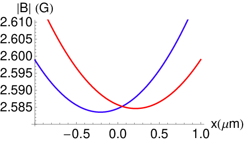
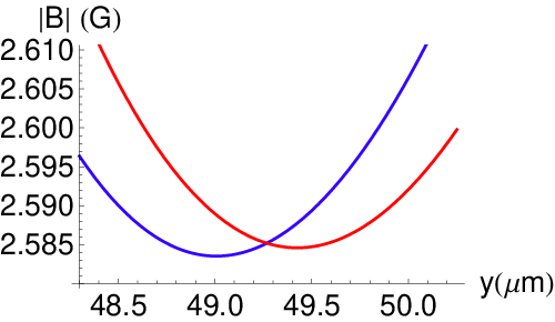
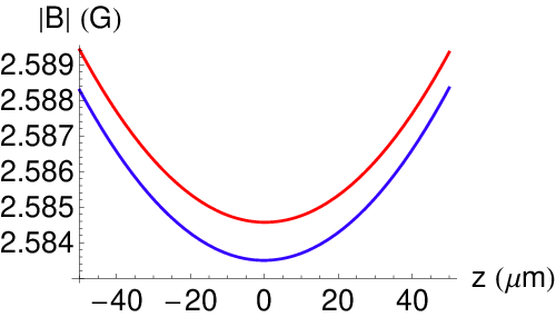
The upper graphs in Figure 1 show how the total magnetic field strength $|B|$ varies along the three Cartesian axes through the centre of the trap. These are calculated using a full numerical model of the apparatus, with $B_{b}=5.9\,$G, directed along $\hat{x}$. The trap along $x$ repeats every $110\,\mu$m because of the periodic magnetisation of the videotape, but only one of these is shown as only one trap is used in the experiments. Along $y$, we see an asymmetric trap, with a strong repulsive wall as the videotape is approached and an asymptote far from the tape that is equal to the total bias field strength. Along $z$, there is the weak trapping due to the inhomogeneous axial bias field.

We load one such trap using an experimental sequence similar to that described in [17]. The temperature of the atom cloud depends on the bias field and ranges from $13\,\mu$K at $B_{b}=5.9\,$G up to $130\,\mu$K at $B_{b}=35.6\,$G. We then add a modulation field $b\cos(2\pi ft)$ along $\hat{x}+\hat{y}$, to displace the trap by a small distance $-\tfrac{b}{kB_{b}}\cos(\omega t)$ along $\hat{x}+\hat{y}$. We choose $b=105\,$mG, which gives a shaking amplitude of $50-300\,$nm over the range of transverse bias fields used. Zooming into the centre of the trap, the three lower graphs in Fig. 1 show the extrema of this modulation. The first two show the (equal) movements along $x$ and $y$ resulting from our particular arrangement of fields. The third shows the absence of movement along $z$ and also illustrates the modulation of the minimum field, due to the variation of $B_{z}$ with transverse displacement of the trap. Since $B_{z}$ affects the transverse trap frequency, this could cause parametric heating, but the effect is considered in [18] and found to be negligible.

With $B_{b}$ initially set at $5.9\,$G, the atoms are shaken for $5\,\mathrm{s}$ and held for $1\,$s, after which the temperature of the trapped cloud is determined by measuring its density distribution along the $z$-direction. This is done using a CCD camera to record the absorption of resonant laser light [17], taking into account the inhomogeneous Zeeman shift of the trapped atoms. The experiment is repeated for a range of shaking frequencies to map out a resonance curve, shown in the leftmost peak of Fig. 2(a). The next two curves are obtained in the same way with $B_{b}=8.9\,$G and $B_{b}=14.8\,$G. At still higher transverse bias fields ($B_{b}=21.9,29.6$ and $35.6\,$G), the atoms are too close to the videotape to yield clean absorption images. In these three cases the trap is moved away from the surface by lowering the bias to $3\,$G over $3\,$s before taking the image. This weakens the trap, thereby cooling the cloud, and it is the lower temperature in this final trap that we plot in Fig. 2(a).

These temperature resonances show that the atoms absorb energy most efficiently near a particular frequency. In the case of a one-dimensional harmonic trap, the physics would be that of a driven, weakly damped harmonic oscillator, whose Lorentzian resonance would be centred on the oscillator frequency with a width given by the collision rate. The actual widths are much greater than the collision rate, but nevertheless, motivated by this thought, we fit a Lorentzian to each resonance curve and plot the centre frequencies (the red squares) as a function of $B_{b}$ in Fig. 3. For comparison, the line in Fig. 3 shows the frequency of small transverse oscillations, given by Eq. 1, with $B_{z}$ evaluated at the centre of the trap for each value of transverse bias. The data points lie below this line because (i) the most energetic atoms move out of the region of small ${x,y}$ where the harmonic approximation of Eq. (1) is valid and (ii) the atoms are also displaced from the centre along $z$, where the increased value of $B_{z}$ reduces the radial frequency. These effects also produce inhomogeneous broadening of the temperature resonances, making them wider for the hotter clouds at higher bias fields, as seen in Fig. 2(a).

Numerically integrating the equations of motion in the full trap potential, we have calculated the period of oscillation along the $x$ direction through the centre of the trap. The inverse of this is plotted as a function of amplitude $A_{x}$ by the solid lines in Fig. 4, the upper(lower) panel being for the case of $B_{b}=5.9(35.6)\,$G. At small amplitude, the frequency coincides with the harmonic approximation indicated by the dotted line. At large amplitude, the potential approaches that of linear trap, and the frequency tends correspondingly to $\tfrac{1}{4}\sqrt{\mu_{B}kB_{b}/(2mA_{x})}$, indicated by the dashed line. The filled circles(squares) mark the rms radius of the cloud in this direction before(after) resonant heating. These show that the atoms explore the anharmonic region of the transverse trap even before the cloud is heated, and move further into this region after heating. These frequency shifts are larger when the bias field is larger. Figure 5 shows how axial displacement from the centre of the trap lowers the harmonic frequency for small transverse oscillations. The essence of this effect is already captured in Eq. (1) through the dependence of $f_{r}$ on $B_{z}$, but here we show the result of the full numerical model of our experiment. Again, the circles(squares) represent the rms size, this time along $z$ before(after) heating. Both of these mechanisms contribute appreciably to the inhomogeneous broadening seen in Fig. 2(a) and the lowering of the trap frequency seen in Fig. 3.

For a more quantitative understanding of the resonances it is necessary to build a dynamical model that allows the atoms to collide. In the next section we develop such a model and use it to simulate the data presented in Fig. 2(a).

We have measured the temperature rise in a cigar-shaped cloud of cold atoms after shaking it sinusoidally in the transverse direction. Unlike most previous measurements, we have modulated the position of the trap, not its curvature. We have recorded temperature resonances as a function of frequency for several values of the bias field that controls the curvature of the transverse trapping potential. Essential to the interpretation of our measurements is the understanding that, at the temperatures involved, atoms oscillate with a wide range of transverse frequencies in the trap and hence that the central frequencies of the observed resonances lie below the calculated harmonic frequencies for small oscillations.

We have developed a simple numerical model that has provided a clear quantitative understanding of the driven dynamics. When compared with other models and simulations in the literature, this provides one of the most detailed and complete attempts to reproduce the observed resonances. No other models include both the collisions between particles and the anharmonicity of the trapping potential, yet both of these are shown to be essential for a full understanding of the behaviour.