Shape identification and classification in echolocationThanks: This work was supported by the ERC Advanced Grant Project MULTIMOD–267184.

Habib Ammari ^†^†thanks: Department of Mathematics and Applications, Ecole Normale Supérieure, 45 Rue d’Ulm, 75005 Paris, France (habib.ammari@ens.fr, tran@dma.ens.fr, han.wang@ens.fr). Minh Phuong Tran²²footnotemark: 2 Han Wang²²footnotemark: 2

Abstract

The paper aims at proposing the first shape identification and classification algorithm in echolocation. The approach is based on first extracting geometric features from the reflected waves and then matching them with precomputed ones associated with a dictionary of targets. The construction of such frequency-dependent shape descriptors is based on some important properties of the scattering coefficients and new invariants. The stability and resolution of the proposed identification algorithm with respect to measurement noise and the limited-view aspect are analytically and numerically quantified.

Mathematics Subject Classification (MSC2000): 35R30, 35B30.

Keywords: echolocation, shape classification, scattering coefficients, frequency-dependent shape descriptors.

•

1 Introduction

Echolocation is a form of acoustics that uses active sonar to locate and identify targets. Many animals, such as bats and dolphins, use this method to avoid collisions, to select, identify, and attack preys, and to navigate by emitting sounds and then analyzing the reflected waves [18, 19]. Animals with the ability of echolocation rely on multiple receivers to allow a better perception of the targets’ distance and direction. By noting a difference in sound level and the delay in arrival time of the reflected sound, the animal determines the size and the location of the target. Moreover, the echolocating animal is able to learn how to identify certain targets and discriminate them from all other targets. As far as we know, shape identification and classification in echolocation is not well understood yet. It is the purpose of this paper to develop the first shape identification algorithm in echolocation. We explain how to identify and classify a target, knowing by advance that the latter belongs to a certain collection of shapes. The model relies on differential imaging, i.e., by forming an image from the echoes due to targets at multiple frequencies, and physics-based classification. Considering a multistatic configuration, we first locate the target using a specific location search algorithm. Then, we extract frequency-dependent scattering coefficients of the target from the perturbation of the echoes using a least-squares algorithm. Computing the invariants under rigid motions and scaling from the extracted features yields shape descriptors. Finally, a target is classified by comparing its invariants with those of a set of learned shapes at multiple frequencies.

The main application we have in mind is an improved autonomous navigation using acoustic waves. It is challenging to equip autonomous robots with echolocation perception and provide them, by mimicking echolocating animals, with acoustic imaging and classification capabilities [16].

The present paper extends our recent results on shape description and perception in electrosensing [2, 3]. For the conductivity equation, the concept of generalized polarization tensors [9, 10, 12, 13] has been successfully used for shape identification and classfication [3, 5, 8]. Invariants with respect to rigid transformations and scaling for the generalized polarization tensors in two and three dimensions have been derived [3, 6].

The paper is organized as follows. In Section 2 we first recall the small-volume framework [10, 14, 15, 17, 20] for imaging acoustic targets. In Section 3 we recover the scattering coefficients from multistatic measurements using a least-squares method and estimate the resolving power of the reconstruction. In Section 4 we construct shape descriptors for multiple frequencies based on scaling, rotation, and translation properties of the scattering coefficients. In Section 5, we illustrate numerically on test examples the perfomance of the proposed classification algorithm and its stability with respect to measurement noise and the limited-view aspect. A few concluding remarks are given in the last section.

2 Problem formulation

Let $D\subset\mathbb{R}^{2}$ be a bounded domain with Lipschitz boundary $\partial D$ . We denote by $\varepsilon_{*}$ the electric permittivity and $\mu_{*}$ the magnetic permeability of $D$ , and $\varepsilon_{0},\mu_{0}$ the electric permittivity and the magnetic permeability of the background medium $\mathbb{R}^{2}\setminus\bar{D}$ , respectively. Then we introduce

\displaystyle\varepsilon=\left\{\begin{array}[]{ll}\varepsilon_{0}&x\in\mathbb{R}^{2}\setminus\bar{D},\\ \varepsilon_{*}&x\in D,\end{array}\right.,\ \ \mu=\left\{\begin{array}[]{ll}\mu_{0}&x\in\mathbb{R}^{2}\setminus\bar{D},\\ \mu_{*}&x\in D,\end{array}\right.

and set $k=\omega\sqrt{\varepsilon_{*}\mu_{*}}$ and $k_{0}=\omega\sqrt{\varepsilon_{0}\mu_{0}}$ , where $\omega$ is the operating frequency.

2.1 Helmholtz equation

Let $\Gamma_{k}$ be the fundamental solution to the Helmholtz equation:

(\Delta+k^{2})\Gamma_{k}(x)=\delta_{0}

(5)

subject to the Sommerfield outgoing radiation condition. In two dimensions, $\Gamma_{k}$ is given by

\Gamma_{k}(x)=-\frac{i}{4}H_{0}^{(1)}(k\mathopen{|}x\mathclose{|})

(6)

with $H_{0}^{(1)}$ being the Hankel function of the first kind of order 0.

We consider the scattered wave $u$ , that is, the solution to following equation:

\begin{cases}\nabla\cdot\displaystyle{\frac{1}{\mu}}\nabla u+\omega^{2}\varepsilon u=0\qquad{\rm in}\,\,\mathbb{R}^{2},\\ (u-U)\,\,\,{\rm satisfies\,\,the\,\,outgoing\,\,radiation\,\,condition},\end{cases}

(7)

where $U$ is a solution to $(\Delta+k_{0}^{2})U=0$ .

2.1.1 Layer potentials and representation of the solution

The solution $u$ to (7) admits an integral representation. For this, we introduce the single layer potential as follows:

{\mathcal{S}_{D}^{k}}\left(\phi\right)(x)=\int_{\partial D}{\Gamma_{k}(x,y)\phi(y)d\sigma(y)},\qquad x\in\mathbb{R}^{2},

(8)

where $\phi\in L^{2}(\partial D)$ . The following jump formula holds [10]:

\displaystyle{\left.\frac{\partial\mathcal{S}_{D}^{k}[\phi]}{\partial\nu}\right|_{\pm}}(x)=\left(\pm\displaystyle{\frac{1}{2}}I+(\mathcal{K}^{k}_{D})^{*}\right)[\phi](x)\qquad{\rm a.e.}\quad x\in\partial D,

(9)

where $f|_{+}$ and $f|_{-}$ denote respectively the limit on $\partial D$ from the outside and the inside of $D$ along the normal direction, and ${\partial}/{\partial}\nu$ denotes the normal derivative. Here, ${\left(\mathcal{K}_{D}^{k}\right)^{*}}$ is the Neumann-Poincaré operator defined by

(\mathcal{K}^{k}_{D})^{*}[\phi](x)=\int_{\partial D}{\displaystyle{\frac{\partial\Gamma_{k}(x,y)}{\partial\nu_{x}}}\phi(y)d\sigma(y)}

(10)

with $\nu_{x}$ being the outward normal vectors of $\partial D$ at $x$ . Then the following system admits a unique solution $(\varphi,\psi)\in L^{2}(\partial D)\times L^{2}(\partial D)$ [9]:

\begin{cases}{\mathcal{S}_{D}^{k}}\left(\varphi\right)-{\mathcal{S}_{D}^{k_{0}}}\left(\psi\right)=U&\text{ on }{\partial}D,\\ \displaystyle{\frac{1}{\mu_{*}}\left.{{\frac{\partial{{\mathcal{S}_{D}^{k}}\left(\varphi\right)}}{\partial\nu}}}\right|_{-}-\frac{1}{\mu_{0}}\left.{{\frac{\partial{{\mathcal{S}_{D}^{k_{0}}}\left(\psi\right)}}{\partial\nu}}}\right|_{+}=\frac{1}{\mu_{0}}{\frac{\partial{U}}{\partial\nu}}}&\text{ on }{\partial}D,\end{cases}

(11)

provided that $k_{0}^{2}$ is not a Dirichlet eigenvalue for $-\Delta$ on $D$ . Moreover, the solution $u$ to (7) can be written as

u(x)=\begin{cases}U(x)+{\mathcal{S}_{D}^{k_{0}}}\left(\psi\right)(x),\qquad x\in\mathbb{R}^{2}\setminus\bar{D},\\ {\mathcal{S}_{D}^{k}}\left(\varphi\right)(x),\qquad x\in D.\end{cases}

(12)

2.1.2 Asymptotic expansion

We first recall Graf’s formula [1]:

H_{0}^{(1)}(k|x-y|)=\sum\limits_{n\in\mathbb{Z}}{H_{n}^{(1)}(k|x|)e^{in\theta_{x}}J_{n}(k|y|)e^{-in\theta_{y}}}\ \text{ for }|x|>|y|,

(13)

where $H_{n}^{(1)}$ is the Hankel function of the first kind of order $n$ defined by

\displaystyle H_{n}^{(1)}(x)=J_{n}(x)+iY_{n}(x),

(14)

and $J_{n},Y_{n}$ are the Bessel function of the first and the second kind of order $n$ , respectively.

Then by plugging Graf’s formula into (12), we obtain an asymptotic form of $u-U$ as $|x|\to\infty$ :

u(x)-U(x)=-\displaystyle{\frac{i}{4}}\sum\limits_{n\in\mathbb{Z}}{H_{n}^{(1)}(k_{0}|x|)e^{in\theta_{x}}\int_{\partial D}J_{n}(k_{0}|y|)e^{-in\theta_{y}}\psi(y)d\sigma(y)}.

(15)

In the following, we use $\mathcal{C}_{m}$ to denote the cylindrical wave of index $m\in\mathbb{Z}$ and of wave number $k_{0}$ , which is defined by

\displaystyle\mathcal{C}_{m}(x)=\mathcal{C}_{m,k_{0}}(x):=J_{m}(k_{0}|x|)e^{im\theta_{x}}.

(16)

2.2 Scattering coefficients

2.2.1 Definition

Let $(\varphi_{m},\psi_{m})$ be the solution to (11) with the cylindrical wave $\mathcal{C}_{m}$ as the source term $U$ . We introduce the scattering coefficients as follows [11].

Definition 2.1.

The scattering coefficients $W_{mn}$ ( $m,n\in\mathbb{Z}$ ) associated with the permittivity and permeability distributions $\varepsilon,\mu$ given by (2) and the frequency $\omega$ are defined by

W_{mn}=W_{mn}[D]=W_{mn}[D,\varepsilon,\mu,\omega]:=\int_{\partial D}{\overline{\mathcal{C}_{n}(y)}\psi_{m}(y)d\sigma(y)}.

(17)

The coefficient $W_{mn}$ decays very fast as the orders $m,n$ increase. In fact, it has been proved in [11] that there is a constant $C_{0}$ depending on $(D,\varepsilon,\mu,\omega)$ such that

\displaystyle\mathopen{|}W_{mn}[D,\varepsilon,\mu,\omega]\mathclose{|}\leq\frac{C_{0}^{\mathopen{|}m\mathclose{|}+\mathopen{|}n\mathclose{|}}}{\mathopen{|}m\mathclose{|}^{\mathopen{|}m\mathclose{|}}\mathopen{|}n\mathclose{|}^{\mathopen{|}n\mathclose{|}}}\,\,\text{ for all }m,n\in\mathbb{Z}.

(18)

2.2.2 Transformation formulas

We introduce the notation for translation, scaling and rotation of a vector $x$ as $x^{z}:=x+z,x^{s}:=sx,x^{\theta}:=R_{\theta}x$ , and those of a shape as

D^{z}:=D+z,D^{s}:=sD,D^{\theta}:=R_{\theta}D,

and define new functions $f^{z},f^{\theta},f^{s}$ so that

f^{z}(x^{z})=f^{\theta}(x^{\theta})=f^{s}(x^{s})=f(x).

Explicit relations exist between the scattering coefficients of $D$ and $D^{z},D^{s},D^{\theta}$ . We will need the following technical lemma:

Lemma 2.1.

We denote by $\psi_{\scriptscriptstyle{U,D}}=\psi_{\scriptscriptstyle{U,D,\omega}}$ the solution to (11) given the domain $D$ , the source term $U$ and the frequency $\omega$ . Then for any $z\in\mathbb{R}^{2}$ , $\theta\in\mathbb{R}$ and $s>0$ :

\displaystyle\psi_{\scriptscriptstyle{U,D}}(x)=\psi_{\scriptscriptstyle{U^{z},D^{z}}}(x^{z})=\psi_{\scriptscriptstyle{U^{\theta},D^{\theta}}}(x^{\theta})=s\psi_{\scriptscriptstyle{U^{s},D^{s},\omega/s}}(x^{s}),\,\forall x\in{\partial}D.

(19)

Proof.

We first prove $\psi_{\scriptscriptstyle{U,D}}(x)=\psi_{\scriptscriptstyle{U^{z},D^{z}}}(x^{z})$ . The following equalities are easily verified:

	$\displaystyle{\mathcal{S}_{D^{z}}^{k}}\left(\phi^{z}\right)(x^{z})$	$\displaystyle={\mathcal{S}_{D}^{k}}\left(\phi\right)(x)\,\text{ for }x\in\mathbb{R}^{2},$		(20)
	$\displaystyle{\left(\mathcal{K}_{D^{z}}^{k}\right)^{*}}\left(\phi^{z}\right)(x^{z})$	$\displaystyle={\left(\mathcal{K}_{D}^{k}\right)^{*}}\left(\phi\right)(x)\,\text{ for }x\in{\partial}D,$

which imply, using the jump formula (9), that if $(\varphi,\psi)$ is the solution to (11), $(\varphi^{z},\psi^{z})$ will be the solution to the following system:

\begin{cases}{\mathcal{S}_{D^{z}}^{k}}\left(\varphi\right)-{\mathcal{S}_{D^{z}}^{k_{0}}}\left(\psi\right)=U^{z}&\text{ on }{\partial}D^{z},\\ \displaystyle{\frac{1}{\mu_{*}}\left.{{\frac{\partial{{\mathcal{S}_{D^{z}}^{k}}\left(\varphi\right)}}{\partial\nu}}}\right|_{-}-\frac{1}{\mu_{0}}\left.{{\frac{\partial{{\mathcal{S}_{D^{z}}^{k_{0}}}\left(\psi\right)}}{\partial\nu}}}\right|_{+}=\frac{1}{\mu_{0}}{\frac{\partial{U^{z}}}{\partial\nu}}}&\text{ on }{\partial}D^{z}.\end{cases}

(21)

Hence we obtain $\psi_{\scriptscriptstyle{U^{z},D^{z}}}(x)=\psi^{z}(x)$ and so forth the first identity in (19). The proof of the identity $\psi_{\scriptscriptstyle{U,D}}(x)=\psi_{\scriptscriptstyle{U^{\theta},D^{\theta}}}(x^{\theta})$ follows analogous arguments and is skipped for brevity.

We prove now $\psi_{\scriptscriptstyle{U,D}}(x)=s\psi_{\scriptscriptstyle{U^{s},D^{s},\omega/s}}(x^{s})$ . Similarly, the following equalities can be verified:

	$\displaystyle s^{-1}{\mathcal{S}_{D^{s}}^{k/s}}\left(\phi^{s}\right)(x^{s})$	$\displaystyle={\mathcal{S}_{D}^{k}}\left(\phi\right)(x)\,\text{ for }x\in\mathbb{R}^{2},\$
	$\displaystyle\frac{{\partial}{\mathcal{S}_{D^{s}}^{k/s}}\left(\phi^{s}\right)(x^{s})}{{\partial}\nu}\bigg\|_{\pm}$	$\displaystyle=\frac{{\partial}{\mathcal{S}_{D}^{k}}\left(\phi\right)(x)}{\partial\nu}\bigg\|_{\pm}\,\text{ for }x\in{\partial}D,$

which implies that if $(\varphi,\psi)$ is the solution to (11), then $(\varphi^{s},\psi^{s})$ will be the solution to the following system:

\begin{cases}{\mathcal{S}_{D^{s}}^{k/s}}\left(\varphi\right)-{\mathcal{S}_{D^{s}}^{k_{0}/s}}\left(\psi\right)=sU^{s}&\text{ on }{\partial}D^{s},\\ \displaystyle{\frac{1}{\mu_{*}}\left.{{\frac{\partial{{\mathcal{S}_{D^{s}}^{k/s}}\left(\varphi\right)}}{\partial\nu}}}\right|_{-}-\frac{1}{\mu_{0}}\left.{{\frac{\partial{{\mathcal{S}_{D^{s}}^{k_{0}/s}}\left(\psi\right)}}{\partial\nu}}}\right|_{+}=\frac{1}{\mu_{0}}{\frac{\partial{\left(sU^{s}\right)}}{\partial\nu}}}&\text{ on }{\partial}D^{s}.\end{cases}

(22)

Hence, we obtain $\psi_{\scriptscriptstyle{sU^{s},D^{s},\omega/s}}(x)=\psi^{s}(x)$ , and so forth the last identity in (19) by noticing that $\psi_{\scriptscriptstyle{sU^{s},D^{s},\omega/s}}(x)=s\psi_{\scriptscriptstyle{U^{s},D^{s},\omega/s}}(x)$ . ∎

Proposition 2.2.

For any $z\in\mathbb{R}^{2},\theta\in[0,2\pi),s>0$ , the following relations hold:


$\displaystyle W_{mn}[D^{z}]$	$\displaystyle=\sum_{a,b\in\mathbb{Z}}{\mathcal{C}_{a}(z)}\overline{\mathcal{C}_{b}(z)}W_{m-a,n-b}[D],$	(23a)
$\displaystyle W_{mn}[D^{\theta}]$	$\displaystyle=e^{i(m-n)\theta}W_{mn}[D],$	(23b)
$\displaystyle W_{mn}[D^{s},\varepsilon,\mu,\omega]$	$\displaystyle=W_{mn}[D,\varepsilon,\mu,s\omega].$	(23c)

Proof.

We establish only (23a) here, and the identities (23b) and (23c) can be proved in a similar way using Lemma 2.1 and change of variables.

We write $\psi_{\scriptscriptstyle{\mathcal{C}_{m},D}}(y):=\psi_{m}(y)$ in order to highlight the dependence on $\mathcal{C}_{m}$ and $D$ , and recall the identity [7]:

\displaystyle\mathcal{C}_{m}(x+y)=\sum_{l\in\mathbb{Z}}\mathcal{C}_{l+m}(x)\overline{\mathcal{C}_{l}(-y)}.

(24)

Then from Lemma 2.1 and by the principle of superposition, it follows that

\displaystyle\psi_{\scriptscriptstyle{\mathcal{C}_{m},D}}(y)=\psi_{\scriptscriptstyle{\mathcal{C}^{z}_{m},D^{z}}}(y^{z})=\sum_{l\in\mathbb{Z}}\overline{\mathcal{C}_{l}(z)}\psi_{\scriptscriptstyle{\mathcal{C}_{l+m},D^{z}}}(y^{z}).

(25)

By the change of variables $y\rightarrow y-z$ in (17) and by substituting (25), we get

	$\displaystyle W_{mn}[D]$	$\displaystyle=\int_{{\partial}D}\overline{\mathcal{C}_{n}(y)}\psi_{\scriptscriptstyle{\mathcal{C}_{m},D}}(y)d\sigma(y)=\sum_{a,b\in\mathbb{Z}}\overline{\mathcal{C}_{a}(z)}{\mathcal{C}_{b}(z)}\int_{{\partial}D^{z}}\overline{\mathcal{C}_{b+n}(y)}\psi_{\scriptscriptstyle{\mathcal{C}_{a+m},D^{z}}}(y)d\sigma(y)$
		$\displaystyle=\sum_{a,b\in\mathbb{Z}}\overline{\mathcal{C}_{a}(z)}{\mathcal{C}_{b}(z)}W_{a+m,b+n}[D^{z}],$

which is equivalent to

\displaystyle W_{mn}[D^{z}]=\sum_{a,b\in\mathbb{Z}}\overline{\mathcal{C}_{a}(-z)}{\mathcal{C}_{b}(-z)}W_{a+m,b+n}[D].

Therefore, we obtain (23a) by the fact $\mathcal{C}_{a}(-z)=\overline{\mathcal{C}_{-a}(z)}$ . Finally, we remark that the sum in (23) converges absolutely, due to the decay (18) of $W_{mn}$ and the decay (46) of the Bessel functions. ∎

Using (19) and (20), we prove easily the identity:

\displaystyle{\mathcal{S}_{D}^{k_{0}}}\left(\psi_{\scriptscriptstyle{U,D}}\right)(x)={\mathcal{S}_{D^{z}}^{k_{0}}}\left(\psi_{\scriptscriptstyle{U^{z},D^{z}}}\right)(x^{z})\,\text{ for }x\in\mathbb{R}^{2}.

Consequently, by the integral representation formula (12) this yields the following result.

Corollary 2.3.

Let $u_{\scriptscriptstyle{U,D}}$ be the solution to (11) given the domain $D$ and the source term $U$ . Then for any $z\in\mathbb{R}^{2}$ :

\displaystyle u_{\scriptscriptstyle{U,D}}(x)-U(x)=u_{\scriptscriptstyle{U^{z},D^{z}}}(x^{z})-U^{z}(x^{z}),\ \forall\,x\in\mathbb{R}^{2}\setminus\bar{D}.

(26)

3 Reconstruction of scattering coefficients and stability analysis

In this section we investigate the reconstruction of scattering coefficients from the measurements, and analyze the stability of the reconstruction. We consider a multistatic configuration [7]. Formally, let $u_{s}$ be the solution to (7) corresponding to the source term $U_{s}$ for $s=1,2\ldots N_{s}$ , and $\{x_{r}\}$ for $r=1,2,...,N_{r}$ be the set of receivers. The multistatic response matrix (MSR) $\mathbf{V}:=(V_{sr})_{sr}$ is defined by

V_{sr}:=u_{s}(x_{r})-U_{s}(x_{r})\quad{\rm for}\quad r=1\ldots N_{r},\text{ and }s=1\ldots N_{s}.

(27)

The entry $V_{sr}$ is the measurement recorded by the $r$ -th receiver when the $s$ -th source $U_{s}$ is in use.

3.1 Full aperture acquisition

In the following, we adopt a circular acquisition system using plane waves, which refers to the situation that the receivers $x_{r}$ are uniformly distributed on a circle of radius $R$ and centered at $z_{0}$ (typically, $z_{0}$ can be obtained using some localization algorithm and we assume that $z_{0}$ is close to the center of $D$ ), and the sources are plane waves with equally distributed wave direction; see Figure 4 (a). More specifically, for the $r$ -th receiver we have $\mathopen{|}x_{r}-z_{0}\mathclose{|}=R$ and the angle $\theta_{r}:=\theta_{x_{r}-z_{0}}=2\pi r/N_{r}$ , where as the $s$ -th plane wave source is given by

\displaystyle U_{s}(x)=e^{ik_{0}\xi_{s}\cdot x}

(28)

with the unit vector $\xi_{s}$ satisfying $\theta_{s}:=\theta_{\xi_{s}}=2\pi s/N_{s}$ . Thanks to (26), we have

\displaystyle V_{sr}=u_{\scriptscriptstyle{U_{s},D}}(x_{r})-U_{s}(x_{r})=u_{\scriptscriptstyle{U_{s}^{-z_{0}},D^{-z_{0}}}}(x_{r}-z_{0})-U_{s}^{-z_{0}}(x_{r}-z_{0}),

(29)

which means that the measurement recorded at $x_{r}$ given the inclusion $D$ and the source $U_{s}$ is the same as that recorded at $x_{r}-z_{0}$ given the inclusion $D^{-z_{0}}$ and the source $U_{s}^{-z_{0}}$ .

3.2 Linear system of scattering coefficients

We deduce from (29) a linear system involving $W_{mn}$ . Recall first the Jacobi-Anger decomposition of plane waves:

U_{s}^{-z_{0}}(x)=e^{ik_{0}\xi_{s}\cdot(x+z_{0})}=e^{ik_{0}\xi_{s}\cdot z_{0}}\sum\limits_{m\in\mathbb{Z}}{e^{im(\frac{\pi}{2}-\theta_{s})}\mathcal{C}_{m}(x)},

(30)

and by the principle of superposition, the solution $\psi_{\scriptscriptstyle{U_{s}^{-z_{0}},D^{-z_{0}}}}$ to (11) given the inclusion $D^{-z_{0}}$ and the source $U_{s}^{-z_{0}}$ reads:

\displaystyle\psi_{\scriptscriptstyle{U_{s}^{-z_{0}},D^{-z_{0}}}}(x)=e^{ik_{0}\xi_{s}\cdot z_{0}}\sum_{m\in\mathbb{Z}}{e^{im(\frac{\pi}{2}-\theta_{s})}\psi_{\mathcal{C}_{m},D^{-z_{0}}}(x)}.

(31)

On the other hand, we assume $R$ large enough so that $R>\mathopen{|}y\mathclose{|}$ for $y\in{\partial}D^{-z_{0}}$ and Graf’s formula (13) holds with $x$ replaced by $x_{r}-z_{0}$ . Then we apply the asymptotic expansion (15) on the last term of (29), by substituting (31), to finally obtain

	$\displaystyle V_{sr}$	$\displaystyle=-\displaystyle{\frac{i}{4}}\sum\limits_{n\in\mathbb{Z}}H_{n}^{(1)}(k_{0}R)e^{in\theta_{r}}\sum_{m\in\mathbb{Z}}e^{ik_{0}\xi_{s}\cdot z_{0}}{e^{im(\frac{\pi}{2}-\theta_{s})}\int_{\partial D^{-z_{0}}}\overline{\mathcal{C}_{n}(y)}\psi_{\mathcal{C}_{m},D^{-z_{0}}}(y)}d\sigma(y)$
		$\displaystyle=-\displaystyle{\frac{i}{4}}\sum\limits_{n\in\mathbb{Z}}H_{n}^{(1)}(k_{0}R)e^{in\theta_{r}}\sum_{m\in\mathbb{Z}}e^{ik_{0}\xi_{s}\cdot z_{0}}e^{im(\frac{\pi}{2}-\theta_{s})}W_{mn}[D^{-z_{0}}].$		(32)

This motivates us to introduce the constants $A_{sm}$ and $B_{rn}$ :

A_{sm}=e^{ik_{0}\xi_{s}\cdot z_{0}}e^{im(\frac{\pi}{2}-\theta_{s})};\quad B_{rn}=\displaystyle{\frac{i}{4}}\overline{H_{n}^{(1)}(k_{0}R)}e^{-in\theta_{r}},\quad m,n\in\mathbb{Z},

(33)

and rewrite (32) as

\displaystyle V_{sr}=\sum_{m,n\in\mathbb{Z}}A_{sm}{W}_{mn}[D^{-z_{0}}]{(B^{H})}_{nr},

(34)

where $B^{H}$ denotes the Hermitian conjugate transpose of $B$ .

3.2.1 Connection with the far-field pattern

The far-field pattern (the scattering amplitude) when the incident field is the plane wave $U(x)=e^{ik_{0}\xi\cdot x},\mathopen{|}\xi\mathclose{|}=1$ at the frequency $\omega$ , is a two-dimensional $2\pi$ -periodic function $A^{\infty}_{D}(\cdot;\omega)$ defined to be [11]

\displaystyle A^{\infty}_{D}({(\theta_{\xi},\theta_{x})}^{\top};\omega)=\int_{{\partial}D}e^{-ik_{0}\mathopen{|}y\mathclose{|}\cos(\theta_{x}-\theta_{y})}\psi_{\scriptscriptstyle{U,D}}(y)d\sigma(y)

(35)

with $\theta_{\xi},\theta_{x}\in[0,2\pi]$ being respectively the angle of $\xi$ and $x$ in polar coordinates.

In particular, for the circular acquisition system mentioned in Section 3.1 the following relation holds between the MSR and the far-field pattern.

Proposition 3.1.

For a circular acquisition system entered at $z_{0}$ and the radius of the measurement circle $R\to+\infty$ :

\displaystyle\mathopen{|}V_{sr}\mathclose{|}\simeq\frac{1}{\sqrt{8\pi k_{0}R}}\left|A^{\infty}_{D^{-z_{0}}}({(\theta_{s},\theta_{r})}^{\top};\omega)\right|.

(36)

Moreover, there exists a constant $C=C(k_{0},k,D^{-z_{0}})$ such that

\displaystyle\mathopen{|}V_{sr}\mathclose{|}\leq C\left(\frac{\mathopen{|}{\partial}D\mathclose{|}}{\sqrt{R}}\right)\ \text{ when }R\rightarrow+\infty.

(37)

Proof.

Recall the following asymptotic of the Hankel function

\displaystyle H_{0}^{(1)}(t)=\sqrt{\frac{2}{\pi t}}e^{i\left(t-\frac{\pi}{4}\right)}+O(1/t)\ \text{ as }t\rightarrow\infty.

(38)

Substituting in the integral representation of (29), we find

	$\displaystyle V_{sr}$	$\displaystyle={\mathcal{S}_{D^{-z_{0}}}^{k_{0}}}\left(\psi_{\scriptscriptstyle{U_{s}^{-z_{0}},D^{-z_{0}}}}\right)(x_{r})$
		$\displaystyle\simeq-\frac{i}{4}e^{-\frac{\pi i}{4}}e^{ik_{0}R}\sqrt{\frac{2}{\pi k_{0}R}}\int_{{\partial}D^{-z_{0}}}e^{-ik_{0}\mathopen{\|}y\mathclose{\|}\cos(\theta_{x}-\theta_{y})}\psi_{\scriptscriptstyle{U_{s}^{-z_{0}},D^{-z_{0}}}}(y)d\sigma(y),$		(39)

which gives (36) by definition of the far-field pattern after taking the modulus.

It is proved in [9] that there exists a constant $C=C(k,k_{0},D)$ such that the solution $(\phi,\psi)$ of (11) satisfies:

\displaystyle\mathopen{\|}\varphi\mathclose{\|}_{L^{2}({\partial}D)}+\mathopen{\|}\psi\mathclose{\|}_{L^{2}({\partial}D)}\leq C(\mathopen{\|}U\mathclose{\|}_{L^{2}({\partial}D)}+\mathopen{\|}\nabla U\mathclose{\|}_{L^{2}({\partial}D)}).

(40)

For the plane wave source $U_{s}$ , this implies:

\displaystyle\mathopen{\|}\psi_{\scriptscriptstyle{U_{s},D}}\mathclose{\|}_{L^{2}({\partial}D)}\leq C(1+k_{0})\mathopen{|}{\partial}D\mathclose{|}^{1/2}.

Substituting back in (39) and applying Cauchy-Schwartz inequality, we obtain (37). ∎

3.2.2 Truncated linear system

A truncated version of (34) using the first $\mathopen{|}m\mathclose{|},\mathopen{|}n\mathclose{|}\leq K$ terms reads

V_{sr}=\sum_{m=-K}^{K}\sum_{n=-K}^{K}{A_{sm}{W}_{mn}[D^{-z_{0}}]{(B^{H})}_{nr}}+E_{sr},

(41)

where $E_{sr}$ denotes the truncation error. For the fixed expansion-order $K$ , we introduce the matrix $\mathbf{W}=({W}_{mn}[D^{-z_{0}}])_{mn}$ of dimension $(2K+1)\times(2K+1)$ , the source matrix $\mathbf{A}=(A_{sm})_{sm}$ of dimension $N_{s}\times(2K+1)$ and the receiver matrix $\mathbf{B}=(B_{rn})_{rn}$ of dimension $N_{r}\times(2K+1)$ , as well as the truncation error matrix $\mathbf{E}=(E_{sr})_{sr}$ of dimension $N_{s}\times N_{r}$ . Then (41) can be put into a matrix form

\displaystyle\mathbf{V}=\mathbf{A}\mathbf{W}\mathbf{B}^{H}+\mathbf{E}=\mathbf{L}(\mathbf{W})+\mathbf{E},

(42)

where the linear operator $\mathbf{L}:\mathbb{R}^{(2K+1)\times(2K+1)}\rightarrow\mathbb{R}^{N_{s}\times N_{r}}$ is given by

\mathbf{L}(\mathbf{X})=\mathbf{A}\mathbf{X}\mathbf{B}^{H}.

(43)

In practical situations, the data $\mathbf{V}$ may be contaminated by some noise ${\mathbf{N}_{\text{noise}}}$ , thereby modifing (42) to

\mathbf{V}=\mathbf{L}(\mathbf{W})+\mathbf{E}+{\mathbf{N}_{\text{noise}}}.

(44)

We suppose that ${\mathbf{N}_{\text{noise}}}=\sigma_{\text{noise}}\mathbf{N}_{0}$ , where $\sigma_{\text{noise}}>0$ and $\mathbf{N}_{0}$ is a $N_{s}$ -by- $N_{r}$ complex random matrix with independent and identically distributed $\mathcal{N}(0,1)$ entries.

From the bound (37), one can see the size of the measurement $V_{sr}$ is of order ${\mathopen{|}{\partial}D\mathclose{|}}/{\sqrt{R}}$ , hence we define signal-to-noise ratio (SNR) to be

\displaystyle{\text{SNR}}=\frac{\mathopen{|}{\partial}D\mathclose{|}/{\sqrt{R}}}{\sigma_{\text{noise}}}.

(45)

3.3 Bound of the truncation error $E_{sr}$

In this section we estimate the truncation error $E_{sr}$ which will be used later to determine the maximal resolving order $K$ that one can achieve in a noisy environment. The following results will be useful:

•

For a fixed $t$ when $n$ is large, we have the following asymptotic behaviors of the Bessel functions [1]:

\displaystyle J_{n}(t)\simeq\displaystyle{\sqrt{\frac{1}{2\pi|n|}}\left(\frac{et}{2|n|}\right)^{|n|}},\ \ Y_{n}(t)\simeq\displaystyle{-\sqrt{\frac{2}{\pi|n|}}\left(\frac{et}{2|n|}\right)^{-|n|}},

(46)

which implies an upper bound of the Hankel function:

\displaystyle\left|H_{n}^{(1)}(k_{0}R)\right|\lesssim{\left(C_{R}\mathopen{|}n\mathclose{|}\right)^{\mathopen{|}n\mathclose{|}}+\left(C_{R}\mathopen{|}n\mathclose{|}\right)^{-\mathopen{|}n\mathclose{|}}},

(47)

where $C_{R}:=2/(ek_{0}R)$ .

•

For $c>0$ and $k\in\mathbb{N}$ such that $k>c/e$ , the following bound holds:

$\displaystyle\sum_{m>k}\left(\frac{c}{m}\right)^{m}\leq\left(\frac{c}{k}\right)^{k}\left(\frac{1}{1+\ln(k/c)}\right).$ (48)

The proof is given in Appendix A.

Proposition 3.2.

Let $C_{R}$ be the constant defined in (47), and $C_{0}>1$ be the constant in (18) with the shape $D^{-z_{0}}$ . Suppose the radius of measurement circle $R$ satisfies $C_{0}^{2}C_{R}<1$ . Then there exists a sufficiently large truncation order $K$ satisfying $K>C_{0}/(C_{R}e)$ , such that the truncation error $E_{sr}$ at the order $K$ decays as

\displaystyle\mathopen{|}E_{sr}\mathclose{|}=O(\rho^{-K})

(49)

with $\rho=\left(C_{0}^{2}C_{R}\right)^{-1}>1$ a constant depending only on $D^{-z_{0}},\varepsilon,\mu,\omega,$ and $R$ .

Proof.

We separate $E_{sr}$ in three terms as follows:

\displaystyle{E_{sr}}=\left(\sum_{\begin{subarray}{c}|m|\leq K\\ |n|>K\end{subarray}}+\sum_{\begin{subarray}{c}|n|\leq K\\ |m|>K\end{subarray}}+\sum_{\begin{subarray}{c}|m|>K\\ |n|>K\end{subarray}}\right){A_{sm}W_{mn}(B^{H})_{rn}}=I_{1}+I_{2}+I_{3}.

Let the radius $R$ be sufficiently large so that $C_{0}^{2}C_{R}<1$ . Then by (18) and (47), we can bound $\mathopen{|}I_{1}\mathclose{|}$ by

	$\displaystyle\mathopen{\|}I_{1}\mathclose{\|}$	$\displaystyle\leq\sum_{\|m\|\leq K}\frac{C_{0}^{\mathopen{\|}m\mathclose{\|}}}{\mathopen{\|}m\mathclose{\|}^{\mathopen{\|}m\mathclose{\|}}}\sum_{\|n\|>K}\left\|H^{(1)}_{n}(k_{0}R)\right\|\frac{C_{0}^{\mathopen{\|}n\mathclose{\|}}}{\mathopen{\|}n\mathclose{\|}^{\mathopen{\|}n\mathclose{\|}}}$
		$\displaystyle\lesssim\left(\sum_{\|m\|\leq K}\frac{C_{0}^{\mathopen{\|}m\mathclose{\|}}}{\mathopen{\|}m\mathclose{\|}^{\mathopen{\|}m\mathclose{\|}}}\right)\left(\sum_{\mathopen{\|}n\mathclose{\|}>K}{\left(C_{0}C_{R}\right)^{\mathopen{\|}n\mathclose{\|}}}+\sum_{\mathopen{\|}n\mathclose{\|}>K}\left(\frac{C_{0}/C_{R}}{\mathopen{\|}n\mathclose{\|}^{2}}\right)^{\mathopen{\|}n\mathclose{\|}}\right).$

Up to some factors independent of $K$ , we can bound the first sum in the last expression by $C_{0}^{K}$ , and the second sum by $(C_{0}C_{R})^{K}$ (since $C_{0}C_{R}<C_{0}^{2}C_{R}<1$ ). Furthermore, as a consequence of (48) the last sum can be neglected by choosing

\displaystyle K>C_{0}/(C_{R}e)

sufficiently large. Therefore, we obtain $\mathopen{|}I_{1}\mathclose{|}\lesssim(C_{0}^{2}C_{R})^{K}$ . Proceeding in a similar way one can establish for $I_{2}$ and $I_{3}$ :

\displaystyle\mathopen{|}I_{2}\mathclose{|}\lesssim(C_{0}^{2}C_{R})^{K},\ \text{ and }\mathopen{|}I_{3}\mathclose{|}\lesssim(C_{0}^{2}C_{R})^{K}K^{-K}.

Putting these bounds together gives (49). ∎

3.4 Stability of the linear operator L

Here we show that the operator $\mathbf{L}$ is ill-conditioned for the circular acquisition system mentioned in section 3.2. If $N_{s},N_{r}\geq 2K+1$ , then it can be verified easily that the matrices $\mathbf{A},\mathbf{B}$ defined in (33) are orthogonal:

\displaystyle\mathbf{A}^{H}\mathbf{A}=N_{s}\mathbf{I},\ \text{ and }\mathbf{B}^{H}\mathbf{B}=N_{r}\mathbf{D},

(50)

where $\mathbf{I}$ is the identity matrix of dimension $\left(2K+1\right)\times\left(2K+1\right)$ and the $\left(2K+1\right)\times\left(2K+1\right)$ diagonal matrix

\displaystyle\mathbf{D}=\begin{pmatrix}|d_{-K}|^{2}&0&\ldots&0\\ 0&|d_{-K+1}|^{2}&\ldots&0\\ \vdots&\vdots&\ddots&\vdots\\ 0&0&\ldots&|d_{K}|^{2}\end{pmatrix}\ \ \text{ with }d_{n}=\displaystyle{\frac{i}{4}}{H_{n}^{(1)}(k_{0}R)}.

(51)

Proposition 3.3.

Suppose $N_{s},N_{r}\geq 2K+1$ . The right singular vector of $\mathbf{L}$ is the canonical basis of $\mathbb{R}^{(2K+1)\times(2K+1)}$ , and the $(m,n)$ -th singular value of operator $\mathbf{L}$ is

\lambda_{mn}=\sqrt{N_{s}N_{r}}|d_{n}|,\ \forall\,m,n=-K,\ldots,K.

(52)

Proof.

For $m,n=-K\ldots K$ , let $\mathbf{v}_{mn}$ be the $\left(2K+1\right)\times\left(2K+1\right)$ square matrix

(\mathbf{v}_{mn})_{ij}=\delta_{mi}\delta_{nj},\ \forall\,i,j=-K,\ldots,K.

(53)

We define the inner product of two complex matrices as $\langle A,B\rangle:=\sum_{m,n}(A^{H})_{mn}B_{mn}$ . A simple computation using (50) shows

\displaystyle\langle\mathbf{L}(\mathbf{v}_{mn}),\mathbf{L}(\mathbf{v}_{m^{\prime}n^{\prime}})\rangle=N_{s}N_{r}\langle\mathbf{v}_{mn},\mathbf{v}_{m^{\prime}n^{\prime}}\mathbf{D}\rangle=\delta_{mm^{\prime}}\delta_{nn^{\prime}}N_{s}\,N_{r}\,\mathopen{|}d_{n}\mathclose{|}^{2}.

This proves that the canonical basis $\{\mathbf{v}_{mn}\}_{m,n=-K\ldots K}$ constitutes the right singular vectors of $\mathbf{L}$ . The $(m,n)$ -th singular value of $\mathbf{L}$ is hence given by

\lambda_{mn}=||\mathbf{L}(\mathbf{v}_{mn})||_{F}=\sqrt{N_{s}N_{r}}|d_{n}|,\quad m,n=-K,\ldots,K,

(54)

where $\mathopen{\|}\cdot\mathclose{\|}_{F}$ denotes the Frobenius norm of matrices. The left singular vectors are given by $\mathbf{u}_{mn}:=\mathbf{L}(\mathbf{v}_{mn})/\lambda_{mn}$ . This completes the proof. ∎

3.4.1 Condition number of $\mathbf{L}$

Remark that as $K\rightarrow+\infty$ , $\mathopen{|}d_{K}\mathclose{|}$ diverges, and hence $\mathbf{L}$ is an unbounded operator and the following bound holds for the condition number of $\mathbf{L}$ :

Corollary 3.4.

Under the same assumptions of Proposition 3.3, we have

\displaystyle\mathrm{\text{cond}}\,(\mathbf{L})\lesssim(C_{R}K)^{K}\ \text{ as }K\rightarrow+\infty

(55)

with the constant $C_{R}$ defined in (47).

Proof.

We denote respectively by ${d_{\text{max}}}$ and ${d_{\text{min}}}$ the maximum and the minimum value of $\mathopen{|}d_{n}\mathclose{|}$ for $n=-K\ldots K$ . Using the asymptotic expansion in (46), we obtain

\displaystyle\mathopen{|}d_{n}\mathclose{|}\propto\left|H^{(1)}_{n}(k_{0}R)\right|\simeq\sqrt{\frac{2}{\pi\mathopen{|}n\mathclose{|}}}\left(C_{R}\mathopen{|}n\mathclose{|}\right)^{\mathopen{|}n\mathclose{|}}\ \text{ as }\mathopen{|}n\mathclose{|}\rightarrow+\infty.

(56)

Hence, when $K$ is large, ${d_{\text{max}}}\simeq d_{K}$ and ${d_{\text{min}}}$ is bounded from below. Therefore, the condition number is bounded by

\displaystyle\text{cond}(\mathbf{L})=\frac{{d_{\text{max}}}}{{d_{\text{min}}}}\lesssim(C_{R}K)^{K},

where the underlying constant depends only on ${d_{\text{min}}}$ . ∎

3.5 Least-squares reconstruction

We can reconstruct $\mathbf{W}$ by solving the least-squares problem

\displaystyle\mathbf{W}^{\text{est}}=\operatornamewithlimits{arg\,min}_{\mathbf{W}\in\operatorname{ker}\mathbf{L}^{\bot}}\left\|\mathbf{L}(\mathbf{W})-\mathbf{V}\right\|_{F},

(57)

where $\operatorname{ker}\mathbf{L}$ denotes the kernel of $\mathbf{L}$ . The solution of (57) is given by $\mathbf{W}^{\text{est}}=\mathbf{L}^{\dagger}(\mathbf{V})$ with $\mathbf{L}^{\dagger}$ being the pseudo-inverse of $\mathbf{L}$ . Since the order $K$ satisfies $2K+1<N_{s},N_{r}$ , the matrices $\mathbf{A}$ and $\mathbf{B}$ have full columns rank and both of them have left pseudo-inverses denoted by $\mathbf{A}^{\dagger}$ and $\mathbf{B}^{\dagger}$ , respectively. Then we have the pseudo-inverse formulas

\displaystyle\mathbf{A}^{\dagger}=(\mathbf{A}^{H}\mathbf{A})^{-1}\mathbf{A}^{H},\quad\mathbf{B}^{\dagger}=(\mathbf{B}^{H}\mathbf{B})^{-1}\mathbf{B}^{H}.

(58)

Using the orthogonal property (50) of $\mathbf{A}$ and $\mathbf{B}$ together with (58), we verify that

\displaystyle\mathbf{L}^{\dagger}(\mathbf{V})=\frac{1}{N_{s}N_{r}}\mathbf{A}^{H}\mathbf{V}\mathbf{B}\mathbf{D}^{-1},

(59)

which provides an analytical reconstruction formula for $\mathbf{W}$ .

3.6 Maximal resolving order

Here we give an estimation of the maximal resolving order $K$ that can be reconstructed by (57) as a function of the SNR.

Let $\rho$ be the constant in Proposition 3.2. We work under the assumption

\rho^{-K}\ll\sigma_{\text{noise}}\ll{\mathopen{|}{\partial}D\mathclose{|}}/{\sqrt{R}},

(60)

which is the regime that the measurement noise is much larger than the truncation error but much smaller than the signal (or ${\text{SNR}}\gg 1$ ).

Since $\mathbf{L}$ is injective, $\mathbf{L}^{\dagger}\mathbf{L}=\mathbf{I}$ and from (44) we have

\displaystyle\mathbb{E}(\left|\left(\mathbf{W}^{\text{est}}-\mathbf{W}\right)_{mn}\right|^{2})^{1/2}=\mathbb{E}(\mathopen{|}{\mathbf{L}^{\dagger}(\mathbf{E}+{\mathbf{N}_{\text{noise}}})}_{mn}\mathclose{|}^{2})^{1/2}\leq\mathopen{|}\mathbf{L}^{\dagger}(\mathbf{E})_{mn}\mathclose{|}+\sigma_{\text{noise}}\lambda_{mn}^{-1}\sqrt{N_{s}N_{r}}.

On one hand, by Cauchy-Schwartz inequality and the bound (49):

\displaystyle\mathopen{|}\mathbf{L}^{\dagger}(\mathbf{E})_{mn}\mathclose{|}\leq\lambda_{mn}^{-1}\mathopen{\|}\mathbf{E}\mathclose{\|}_{F}\lesssim\lambda_{mn}^{-1}\sqrt{N_{s}N_{r}}\rho^{-K},

which can be neglected thanks to the left inequality of (60). Therefore, we obtain

\displaystyle\mathbb{E}(\left|\left(\mathbf{W}^{\text{est}}-\mathbf{W}\right)_{mn}\right|^{2})^{1/2}\lesssim\sigma_{\text{noise}}\lambda_{mn}^{-1}\sqrt{N_{s}N_{r}}=\sigma_{\text{noise}}\mathopen{|}d_{n}\mathclose{|}^{-1},

(61)

which decreases to zero for all $m,n\geq K$ as $K\rightarrow+\infty$ , due to (56). Apparently, this seems to imply that the maximal resolving order is infinity. However, from the decay behavior (18) of $W_{mn}$ , it is reasonable to require the reconstruction error to be smaller than the signal level:

\displaystyle\mathbb{E}(\left|\left(\mathbf{W}^{\text{est}}-\mathbf{W}\right)_{mn}\right|^{2})^{1/2}\leq\tau_{0}\frac{C_{0}^{\mathopen{|}m\mathclose{|}+\mathopen{|}n\mathclose{|}}}{\mathopen{|}m\mathclose{|}^{\mathopen{|}m\mathclose{|}}\mathopen{|}n\mathclose{|}^{\mathopen{|}n\mathclose{|}}}

with $\tau_{0}>0$ being a tolerance number. Using (61) at the order $m=n=K$ , this implies

\displaystyle\sigma_{\text{noise}}\frac{1}{\mathopen{|}d_{K}\mathclose{|}}\lesssim\tau_{0}\left(\frac{C_{0}}{K}\right)^{2K},

which yields $\sigma_{\text{noise}}K^{K+1/2}\lesssim\tau_{0}\rho^{-K}$ by (56). Finally, according to the regime (60) and by definition of the SNR, we find

\displaystyle K^{K+1/2}\lesssim\tau_{0}{\text{SNR}},

(62)

and the maximal resolving order is defined as the largest $K$ satisfying (62).

4 Shape descriptor and identification in a dictionary

In this section we construct the shape descriptors based on the scattering coefficients which are invariant to rigid transform. For a collection of standard shapes, we build a frequency-dependent dictionary of shape descriptors and develop a shape identification algorithm in order to identify a shape from the dictionary up to some translation, rotation and scaling. In the following, we denote by $B$ a reference shape of size $1$ centered at the origin, so that the unknown inclusion $D$ is obtained from $B$ by a rotation with angle $\theta$ , a scaling $s>0$ and a translation $z\in\mathbb{R}^{2}$ as $D=z+sR_{\theta}B$ .

4.1 Translation and rotation invariant shape descriptor

The construction of the shape descriptor starts from the formula (23a), where the convolution relationship suggests us to pass to the Fourier domain. It turns out that the Fourier series of $W_{mn}[D]$ is just the far-field pattern $A^{\infty}_{D}$ [11]. The following proposition holds.

Proposition 4.1.

Let $\xi={(\xi_{1},\xi_{2})}^{\top}\in[0,2\pi]^{2}$ . Then, we have

\displaystyle A^{\infty}_{D}(\xi;\omega)=\sum_{m,n\in\mathbb{Z}}W_{mn}[D,\varepsilon,\mu,\omega]e^{im(\frac{\pi}{2}-\xi_{1})}e^{-in(\frac{\pi}{2}-\xi_{2})}.

(63)

Remark 4.1.

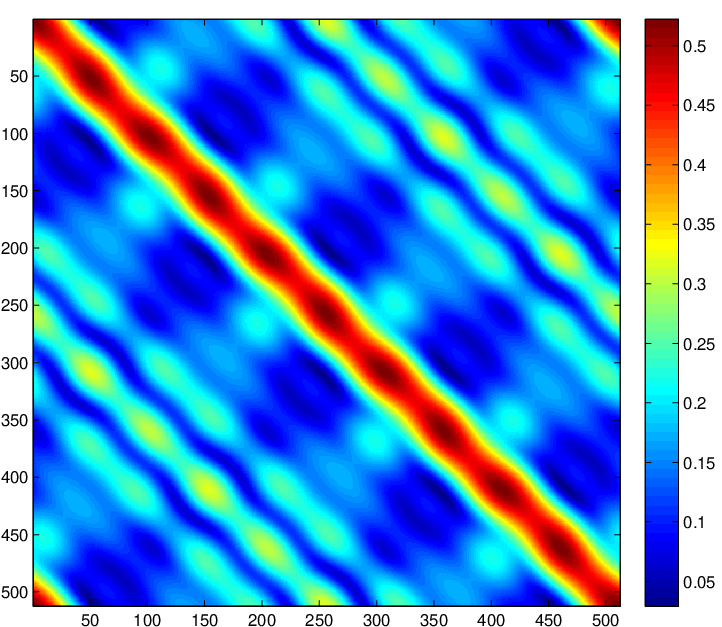
For the circular acquisition system mentioned in Section 3.1, the modulus of the far-field pattern can be read off directly from the measurement when the radius $R$ and the number of sources $N_{s}$ and receivers $N_{r}$ are large, thanks to (36). See Figure 1.

Refer to caption — (a) $\left|V_{sr}\right|$

We emphasize that the Fourier series in (63) converges thanks to the decay (18) of $W_{mn}$ . Then using the translation formula (23a), we establish the relations between the far-field pattern of $D$ and $B$ .

Proposition 4.2.

Let $D=z+sR_{\theta}B$ . We denote by $\theta_{z}$ the angle of $z$ in polar coordinate, and define $\phi_{z}(\xi):=e^{ik_{0}\mathopen{|}z\mathclose{|}\cos(\xi_{1}-\theta_{z})}e^{-ik_{0}\mathopen{|}z\mathclose{|}\cos(\xi_{2}-\theta_{z})}$ . Then, we have

\displaystyle A^{\infty}_{D}(\xi;\omega)=\phi_{z}(\xi)\,A^{\infty}_{B}(\xi_{\theta};s\omega)\ \text{ with }\xi_{\theta}:=\xi-{(\theta,\theta)}^{\top}.

(64)

Proof.

By the transformation formulas (23), we have

	$\displaystyle W_{mn}[D,\varepsilon,\mu,\omega]$	$\displaystyle=\sum_{a,b\in\mathbb{Z}}\mathcal{C}_{a}(z)\overline{\mathcal{C}_{b}(z)}W_{m-a,n-b}[sR_{\theta}B,\varepsilon,\mu,\omega]$
		$\displaystyle=\sum_{a,b\in\mathbb{Z}}\mathcal{C}_{a}(z)\overline{\mathcal{C}_{b}(z)}e^{i(m-a)\theta}e^{-i(n-b)\theta}W_{m-a,n-b}[B,\varepsilon,\mu,s\omega].$		(65)

Using the Jacobi-Anger expansion, the Fourier series of the cylindrical wave reads:

\displaystyle\sum_{a\in\mathbb{Z}}\mathcal{C}_{a}(z)e^{ia(\frac{\pi}{2}-\xi_{1})}=\sum_{a\in\mathbb{Z}}J_{a}(k_{0}\mathopen{|}z\mathclose{|})e^{ia(\frac{\pi}{2}-(\xi_{1}-\theta_{z}))}=e^{ik_{0}\mathopen{|}z\mathclose{|}\cos(\xi_{1}-\theta_{z})}.

Therefore, computing the Fourier series on the both sides of (65) yields (64). ∎

Hereafter, we illustrate the descriptor construction based on the scattering amplitude. We define the following quantity:

\displaystyle\mathcal{S}_{D}(v;\omega):=\int_{[0,2\pi]^{2}}\left|A^{\infty}_{D}(\xi;\omega){A^{\infty}_{D}(\xi-v;\omega)}\right|d\xi.

(66)

More precisely, taking the modulus on $A^{\infty}_{D}$ removes the effect of the translation, and the auto-correlation in $\xi$ removes that of the rotation. In fact, using (64):

\displaystyle\mathcal{S}_{D}(v;\omega)=\int_{[0,2\pi]^{2}}\mathopen{|}A^{\infty}_{B}(\xi_{\theta};s\omega)A^{\infty}_{B}(\xi_{\theta}-v;s\omega)\mathclose{|}d\xi=\mathcal{S}_{B}(v;s\omega),

(67)

where the last identity comes from the periodicity in $\xi$ of $A^{\infty}_{B}(\xi;\omega)$ . We name (66) the shape descriptor. The shape descriptor $\mathcal{S}_{D}(v;\omega)$ is invariant to any translation and rotation. Remark that for fixed $\omega$ , it carries the information of the far-field pattern of the shape, while for fixed $v\in[0,2\pi]^{2}$ , it shows how the far-field pattern varies as a function of the frequency.

4.2 Scale estimation

From $\mathcal{S}_{D}(v;\omega)$ we could hopefully construct, at least formally, some quantities $\mathcal{I}_{D}(v)$ being further invariant to the scaling, and obtain in that way shape descriptors easily adapted for the purpose of identification like in [3]. For example, one may consider the Hilbert transform in $\omega$ of $\mathcal{S}_{D}$ :

\displaystyle\mathcal{I}_{D}(v):=\int_{0}^{+\infty}{\frac{\mathcal{S}_{D}(v;\omega)}{\omega}}d\omega,

(68)

which is invariant to any translation, rotation and scaling, since

\displaystyle\mathcal{I}_{D}(v)=\int_{0}^{+\infty}{\frac{\mathcal{S}_{B}(v;s\omega)}{\omega}}d\omega=\int_{0}^{+\infty}{\frac{\mathcal{S}_{B}(v;\omega)}{\omega}}d\omega=\mathcal{I}_{B}(v).

(69)

Not to mention the well-definedness of (68), let us point out immediately the physical infeasibility of such kind of quantities, whatever the method in use. In fact, the frequency $\omega$ is coupled with the scaling factor $s$ in the relation (67), hence if the knowledge of $\mathcal{S}_{D}(v;\omega)$ in the frequency $\omega$ is bounded away from $0$ or infinity, then it is not possible to construct an $\mathcal{I}_{D}$ being invariant to arbitrary scaling factor $s\in\mathbb{R}^{+}$ , which would require the frequency at 0 or infinity.

4.2.1 Determine $s$ by lookup table

We assume that the physical operating frequency $0<{\omega_{\text{min}}}\leq\omega\leq{\omega_{\text{max}}}<\infty$ , and $0<{s_{\text{min}}}\leq s\leq{s_{\text{max}}}<\infty$ which means the inclusions that we are interested in should not be too small nor to large. Then we can estimate $s$ by solving

\displaystyle s^{\text{est}}=\operatornamewithlimits{arg\,min}_{s\in[{s_{\text{min}}},{s_{\text{max}}}]}\left\{\int_{\omega_{\text{min}}}^{\omega_{\text{max}}}\left(\int_{[0,2\pi]^{2}}[\mathcal{S}_{D}(v;\omega)-\mathcal{S}_{B}(v;s\omega)]\,dv\right)^{2}d\omega\right\},

(70)

which is a lookup table technique since we are seeking the best value of $s$ in the table $\int_{\scriptscriptstyle{[0,2\pi]^{2}}}\mathcal{S}_{B}(v;s\omega)dv$ indexed by $s$ , by comparing with $\int_{\scriptscriptstyle{[0,2\pi]^{2}}}\mathcal{S}_{D}(v;\omega)dv$ . This idea is illustrated in Figure 2. Remark that the functional in (70) is minimized at the value of the true scaling factor, although the minimizer might not be unique.

4.2.2 Numerical implementation of the scaling estimation

Numerically, (70) can be solved approximately by sampling. Let ${N_{\omega}^{\text{dic}}},{N_{\omega}},{N_{v}},N_{s}$ be positive integers. We define $\{\omega^{\text{dic}}_{l},l=0\ldots{N_{\omega}^{\text{dic}}}\}$ uniformly distributed points on $[{\omega^{\text{dic}}_{\text{min}}},{\omega^{\text{dic}}_{\text{max}}}]$ , with ${\omega^{\text{dic}}_{\text{min}}}:={\omega_{\text{min}}}{s_{\text{min}}},{\omega^{\text{dic}}_{\text{max}}}:={\omega_{\text{max}}}{s_{\text{max}}}$ . Similarly, let $\{\omega_{k},k=0\ldots{N_{\omega}}\}$ be uniformly distributed on $[{\omega_{\text{min}}},{\omega_{\text{max}}}]$ , and $\{(v^{1}_{i},v^{2}_{j})^{\top},i,j=1\ldots{N_{v}}\}$ be uniformly distributed in $[0,2\pi]^{2}$ . Then we sample the functions $\mathcal{S}_{B}$ and $\mathcal{S}_{D}$ at discrete positions as follows:

\displaystyle\mathcal{S}^{D}_{ijk}:=\mathcal{S}_{D}({(v^{1}_{i},v^{2}_{j})}^{\top};\omega_{k}),\ \mathcal{S}^{B}_{ijl}:=\mathcal{S}_{B}({(v^{1}_{i},v^{2}_{j})}^{\top};\omega^{\text{dic}}_{l}).

(71)

For $\{s_{t},t=0\ldots,N_{\delta}\}$ uniformly distributed in $[{s_{\text{min}}},{s_{\text{max}}}]$ , we can approximate the functional inside the argmin in (70) by a discrete version:

\displaystyle\mathcal{J}(t;D,B)=\sum_{k=0}^{{N_{\omega}}}\sum_{l\in I_{k}(s_{t})}\left(\sum_{i,j=1}^{N_{v}}\left(\mathcal{S}^{D}_{ijk}-\mathcal{S}^{B}_{ijl}\right)\right)^{2}

(72)

with the index set $I_{k}(s):=\{1\leq l\leq{N_{\omega}^{\text{dic}}},\text{ s.t. }\omega^{\text{dic}}_{l-1}\leq s\omega_{k}\leq\omega^{\text{dic}}_{l}\}$ . Finally, the scaling is estimated through

\displaystyle\varepsilon(D,B)=\min_{t=0\ldots N_{\delta}}\mathcal{J}(t;D,B).

(73)

4.3 Frequency-dependent dictionary and identification algorithm

For a collection of standard shapes $\{B_{n}\}_{n=1\ldots N}$ , we pre-compute the discrete samples $\left(\mathcal{S}^{B_{n}}_{ijl}\right)_{ijl}$ of the shape descriptor $\mathcal{S}_{B_{n}}(v;\omega)$ as in (71) for $v\in[0,2\pi]^{2}$ and $\omega\in[{\omega^{\text{dic}}_{\text{min}}},{\omega^{\text{dic}}_{\text{max}}}]$ . This constitutes a frequency-dependent dictionary of shape descriptors.

Suppose $D$ is the realization of a shape from the dictionary $\{B_{n}\}_{n}$ , up to some unknown translation, rotation and scaling, and the scaling factor satisfies ${s_{\text{min}}}\leq s\leq{s_{\text{max}}}$ . In order to identify $D$ from the dictionary, we compute the discrete samples $\left(\mathcal{S}^{D}_{ijk}\right)_{ijk}$ of the shape descriptor $\mathcal{S}_{D}(v;\omega)$ as in (71), and calculate $\varepsilon(D,B_{n})$ in (73) for all shapes of the dictionary. The true shape is expected to give the best estimation of scaling and to minimize the error $\varepsilon(D,B_{n})$ among all the dictionary elements, thus we take the minimizer of $\{\varepsilon(D,B_{n})\}_{n}$ as the identified shape. This procedure is described in Algorithm 1.

Algorithm 1 Shape identification algorithm

Input:

\left(\mathcal{S}^{D}_{ijk}\right)_{ijk}

of unknown shape

D

\left\{\left(\mathcal{S}^{B_{n}}_{ijk}\right)_{ijk}\right\}_{n}

of the whole dictionary

for

B_{n}

in the dictionary do

\varepsilon_{n}\leftarrow\varepsilon(D,B_{n})

;

n\leftarrow n+1

;

end for

Output: The true dictionary element

n^{*}\leftarrow\operatornamewithlimits{arg\,min}_{n}\varepsilon_{n}

4.4 Shape descriptor with partial far-field pattern

Let us mention an interesting property of $\mathcal{S}_{D}$ at the end of this section. Given $0<\alpha\leq 2\pi$ , we denote the partial far-field pattern $A^{\infty}_{D}$

\displaystyle\widetilde{A^{\infty}_{D}}(\xi;\omega):={A^{\infty}_{D}}(\xi;\omega)\mathbbm{1}(\mathopen{|}\xi_{1}-\xi_{2}\mathclose{|}\leq\alpha),

(74)

i.e. , only the band diagonal of width $\alpha$ in $A^{\infty}_{D}(\cdot;\omega)$ is available. Since

\displaystyle\mathbbm{1}(\mathopen{|}\xi_{1}-\xi_{2}\mathclose{|}\leq\alpha)=\mathbbm{1}(\mathopen{|}(\xi_{1}-\theta)-(\xi_{2}-\theta)\mathclose{|}\leq\alpha),

so for the same reason as in (67) we deduce that

\displaystyle\int_{[0,2\pi]^{2}}\left|\widetilde{A^{\infty}_{D}}(\xi;\omega)\widetilde{A^{\infty}_{D}}(\xi-v;\omega)\right|d\xi=\int_{[0,2\pi]^{2}}\left|\widetilde{A^{\infty}_{B}}(\xi_{\theta};s\omega)\widetilde{A^{\infty}_{B}}(\xi_{\theta}-v;s\omega)\right|d\xi.

Therefore, the shape descriptor $\mathcal{S}_{D}$ computed with $\widetilde{A^{\infty}_{D}}$ is still invariant to translation and rotation. Assuming that the dictionary ${\left(\mathcal{S}^{B_{n}}_{ijk}\right)_{ijk}}$ is also computed using partial far field pattern $\widetilde{A^{\infty}_{B_{n}}}$ of the same constant $\alpha$ , then one can always apply Algorithm 1 for shape identification.

5 Numerical experiments

In the rest of this paper, we present numerical results demonstrating the theoretical framework presented in previous sections. Given a shape $D$ , the overall procedure of a numerical experiment consists of the following steps:

1.

Data simulation. The MSR matrix $\mathbf{V}$ is simulated for a range of frequency $[{\omega_{\text{min}}},{\omega_{\text{max}}}]$ by evaluating the integral representation (12). Then the white noise is of level

$\displaystyle\sigma_{\text{noise}}=\sigma_{0}\mathopen{\|}\mathbf{V}\mathclose{\|}_{F}/\sqrt{N_{s}N_{r}}$

is added as in (44). $\sigma_{0}$ is the percentage of the noise in the measurement and it is proportional to ${\text{SNR}}^{-1}$ .
2.

Reconstruction of scattering coefficients. For each frequency, we reconstruct $\mathbf{W}$ either by solving the least-squares problem (57) (or directly by the formula (59) in case of the full aperture of view). This step is skipped in the case of limited aperture of view, see Section 5.3.
3.

Shape identification. We calculate the shape descriptors and follow the procedure described in Algorithm 1 for identification.

Our dictionary of shapes consists of eight elements as shown in Figure 3. All shapes share the same permittivity $\varepsilon_{*}=3$ and the permeability $\mu_{*}=3$ , while the values of the background are $\varepsilon_{0}=1,\mu_{0}=1$ . The frequency-dependent dictionary of shape descriptors $\left\{\left(\mathcal{S}^{B_{n}}_{ijk}\right)_{ijk}\right\}_{n}$ is computed for the frequency range $[{\omega^{\text{dic}}_{\text{min}}},{\omega^{\text{dic}}_{\text{max}}}]=[0.5\pi,4\pi]$ with ${N_{\omega}^{\text{dic}}}=219$ and ${N_{v}}=512$ . The data are simulated for the operating frequency range $[{\omega_{\text{min}}},{\omega_{\text{max}}}]=[\pi,2\pi]$ with ${N_{\omega}}=109$ and the valid scaling range is $[{s_{\text{min}}},{s_{\text{max}}}]=[0.5,2]$ with $N_{\delta}=751$ .

5.1 Experiment and parameter settings

We generate a circular acquisition system like in Section 3.1 with the radius $R=3$ , and $N_{s}=91$ plane waves as sources and $N_{r}=91$ receivers. For reason of simplicity, we always choose the center $z_{0}=[0,0]^{\top}$ . Figure 4 (a) illustrates this acquisition system.

Another possibility is shown in Figure 4 (b), where the sources and receivers are divided into different groups of aperture angle $\alpha$ such that no intercommunication exists between groups. Such an acquisition is close to that used by the bat. Each group in Figure 4 (b) represents the spatial position of a flying bat’s body, which sends plane waves with limited aperture of wave direction and receives the scattered field via receptors on its body. By flying around the target and taking measurement at many positions, the bat actually acquires data corresponding to the band diagonal part of the MSR matrix of a full aperture of view system, and the width of the band diagonal is the number of the receivers (or proportional to $\alpha$ ).

Figure 5 shows the singular values of the associated operators $\mathbf{L}$ at the operating frequency $\omega=2\pi$ . The stairwise distribution and the increase of singular values with the order $K$ in Figure 5 (a) confirm the theoretical result in (52). It can be seen that at the low-order (e.g. $K\leq 30$ ) the operator $\mathbf{L}$ is numerically well-conditioned. On the contrary, as shown in Figure 5 (b) the situation in the limited aperture of view is dramatically different: the operator is ill-conditioned even for very low-order (e.g. , $K=5$ ), which means the reconstruction of scattering coefficients is highly unstable with such an acquisition system.

5.1.1 Resolving order $K$

The maximal resolving order $K$ given by (62) is an asymptotic bound which holds when both the radius $R$ and $K$ are large, and it might be too pessimistic for the numerical range that we are interested in. In practice, the maximal resolving order can be determined by a tuning procedure. For the system in Figure 4 (a), we vary the noise level and reconstruct the matrix $\mathbf{W}^{\text{est}}$ at different truncation order $K$ . Figure 6 plots the relative error of the least-squares reconstruction $\mathopen{\|}\mathbf{W}^{\text{est}}-\mathbf{W}\mathclose{\|}_{F}/\mathopen{\|}\mathbf{W}\mathclose{\|}_{F}$ as a function of $K$ . It can be seen that in the full aperture case, the reconstruction is rather robust and with $20\%$ of noise the resolving order $K$ can go beyond $30$ by bearing only $10\%$ of error. On the contrary, the limited aperture of view can not provide any stable reconstructions even at very low noise level and small truncation order.

5.2 Shape identification with full aperture of view

Here we present results of shape identification obtained using the full aperture of view setting Figure 4 (a). For each shape $B_{n}$ of the dictionary, we take the three steps mentioned in the beginning of Section 5 on a target $D$ obtained by transform $B_{n}$ with the parameters $z=[-0.5,0.5]^{\top},s=1.5,\theta=\pi/3$ . The order $K$ is set to 30.

The computation of the error $\varepsilon(D,B_{n})$ is represented in Figure 7 by error bars, where the $m$ -th error bar in the $n$ -th group corresponds to the error $\varepsilon(D,B_{m})$ of the identification experiment using the generating shape $B_{n}$ . The error bars are arranged in the same way as in Figure 3. The shortest bar in each group is the identified shape and is marked in green, while the true shape is marked in red in case that the identification fails. It can be seen that the identification succeeded for all shapes with $20\%$ of noise, and it failed only for the rectangle with $40\%$ of noise. The estimated scaling factor computed as in (73) is close to the true value $1.5$ . The discrepancies between them are displayed in Figure 8.

5.3 Shape identification with limited aperture of view

We use a limited view system as Figure 4 (b) of small aperture angle $\alpha$ , with 512 source/receiver groups (the number of sources/receivers in each group is about $512\times\alpha/2\pi$ ) uniformly distributed on a circle of radius $R=10$ around the target. Visually speaking, the modulus of the measurement $\mathopen{|}V_{sr}\mathclose{|}$ is similar to that shown in Figure 1 with all entries set to zero except the band diagonal (in red).

As analyzed in Section 5.1, in this case one can not expect to reconstruct the scattering coefficients with high precision, and consequently compute neither the full far-field pattern via (63) nor the shape descriptor (66). However, thanks to the relation (36) the measurement $\mathopen{|}V_{sr}\mathclose{|}$ gives directly the band diagonal part of the far-field pattern $\mathopen{|}A^{\infty}_{D}\mathclose{|}$ , and one can compute the shape descriptors from the partial far-field pattern hence apply the identification algorithm as described in Section 4.4.

The results of identification with the limited aperture are shown in Figure 9, where all shapes were identified correctly with $\alpha=\pi/3$ and only the square was missed with $\alpha=\pi/6$ . The performance may deteriorate when the dictionary contains more shapes. In that case one should increase the aperture angle and broaden the range of operating frequency $[{\omega_{\text{min}}},{\omega_{\text{max}}}]$ in order to compensate the lose of information in the incomplete far-field pattern.

6 Conclusion

In this paper we presented a framework of shape identification using the frequency-dependent dictionary of shape descriptors, which is invariant to rigid transforms and allows to handle the scaling within certain ranges. The shape descriptor is based on the far-field pattern which can be either computed from the scattering coefficients or read off directly from the measurement. We analyzed the stability of the reconstruction and presented results of identification with both full and limited aperture of view. Our approach in this paper can be used for tracking the location and the orientation of a target from acoustic echoes. The generalization of our work on target tracking in electrosensing [4] to echolocation will be the subject of a forthcoming paper.

Appendix A Proof of (48)

Proof.

Let $f(t):=\left(\frac{c}{t}\right)^{t}$ be defined on $\mathbb{R}^{+}$ . Remark that $f$ is decreasing for $t\geq c/e$ . Therefore, if $k\in\mathbb{N},k>c/e$ , the sum can be bounded by

\displaystyle\sum_{m>k}\left(\frac{c}{m}\right)^{m}\leq\int_{k}^{+\infty}f(t)dt=I.

On the other hand, for any $x>1$ , we define the function $g(t):=f(t)x^{t}$ which attains at $t=cx/e$ its maximum $e^{x(c/e)}=a^{x}$ . Then,

\displaystyle I=\int_{k}^{+\infty}g(t)x^{-t}dt\leq a^{x}\int_{k}^{+\infty}x^{-t}dt=a^{x}\left(\frac{x^{-k}}{\ln x}\right).

Since $x>1$ is arbitrary, we deduce

\displaystyle I\leq\inf_{x>1}a^{x}\left(\frac{x^{-k}}{\ln x}\right)\leq\inf_{x\geq ke/c}a^{x}\left(\frac{x^{-k}}{\ln x}\right)\leq\left(\inf_{x\geq ke/c}a^{x}x^{-k}\right)\left(\frac{1}{\ln(ke/c)}\right).

The function $a^{x}x^{-k}$ is convex on $x>1$ and attains at $x=ke/c>1$ its minimum $(c/k)^{k}$ . Putting everything together, we finally obtain

\displaystyle I\leq\left(\frac{c}{k}\right)^{k}\left(\frac{1}{1+\ln(k/c)}\right)

as desired. ∎

References

[1] M. Abramowitz and I. A. Stegun. Handbook of Mathematical Functions: With Formulars, Graphs, and Mathematical Tables, volume 55. DoverPublications. com, 1964.
[2] H. Ammari, T. Boulier, and J. Garnier. Modeling active electrolocation in weakly electric fish. SIAM J. Imag. Sci., (5):285–321, 2012.
[3] H. Ammari, T. Boulier, J. Garnier, W. Jing, H. Kang, and H. Wang. Target identification using dictionary matching of generalized polarization tensors. Found. Comput. Math., to appear, 2013.
[4] H. Ammari, T. Boulier, J. Garnier, H. Kang, and H. Wang. Tracking of a mobile target using generalized polarization tensors. SIAM J. Imag. Sci., 6:1477–1498, 2013.
[5] H. Ammari, T. Boulier, J. Garnier, and H. Wang. Shape recognition and classification in electro-sensing. arXiv:1302.6384, 2013.
[6] H. Ammari, D. Chung, H. Kang, and H. Wang. Invariance properties of generalized polarization tensors and design of shape descriptors in three dimensions. arXiv:1212.3519, 2012.
[7] H. Ammari, J. Garnier, W. Jing, H. Kang, M. Lim, K. Sø lna, and H. Wang. Mathematical and Statistical Methods for Multistatic Imaging. Springer Verlag, 2013.
[8] H. Ammari, J. Garnier, H. Kang, M. Lim, and S. Yu. Generalized polarization tensors for shape description. Numer. Math., DOI 10.1007/s00211-013-0561-5, to appear, 2013.
[9] H. Ammari and H. Kang. Boundary layer techniques for solving the helmholtz equation in the presence of small inhomogeneities. J. Math. Anal. Appl., 296(1):190–208, 2004.
[10] H. Ammari and H. Kang. Reconstruction of Small Inhomogeneities from Boundary Measurements. Springer Verlag, 2004.
[11] H. Ammari, H. Kang, H. Lee, and M. Lim. Enhancement of near-cloaking. part II: the helmholtz equation. Comm. Math. Phys., (317):485–502, 2013.
[12] H. Ammari, H. Kang, M. Lim, and H. Zribi. The generalized polarization tensors for resolved imaging. part i: Shape reconstruction of a conductivity inclusion. Math. Comp., 81:367–386, 2012.
[13] Y. Capdeboscq, A. B. Karrman, and J.-C. Nédélec. Numerical computation of approximate generalized polarization tensors. Appl. Anal., 91:1189–1203, 2012.
[14] Y. Capdeboscq and M. S Vogelius. A review of some recent work on impedance imaging for inhomogeneities of low volume fraction. Contemporary Mathematics, 362:69–88, 2004.
[15] D. J. Cedio-Fengya, S. Moskow, and M. S. Vogelius. Identification of conductivity imperfections of small diameter by boundary measurements: Continuous dependence and computational reconstruction. Inverse Problems, 14:553–595, 1998.
[16] L. Kleeman and R. Kuc. Mobile robot sonar for target localization and classification. Inter. J. Robotics Research, 14:295–318, 1995.
[17] O. Kwon, J. K. Seo, and J. R. Yoon. A real-time algorithm for the location search of discontinuous conductivities with one measurement. Comm. Pure Appl. Math., 55:1–29, 2002.
[18] J. A. Simmons. Perception of echo phase information in bat sonar. Science, 204:1336–1338, 1979.
[19] J. A. Simmons, M. B. Fenton, and M. J. O’Farrell. Echolocation and pursuit of prey by bats. Science, 203:16–21, 1979.
[20] M. S. Vogelius and D. Volkov. Asymptotic formulas for perturbations in the electromagnetic fields due to the presence of inhomogeneities of small diameter. M2AN Math. Model. Numer. Anal., 34:723–748, 2000.

Shape identification and classification in echolocationThanks: This work was supported by the ERC Advanced Grant Project MULTIMOD–267184.

Abstract

1 Introduction

2 Problem formulation

2.1 Helmholtz equation

2.1.1 Layer potentials and representation of the solution

2.1.2 Asymptotic expansion

2.2 Scattering coefficients

2.2.1 Definition

Definition 2.1.

2.2.2 Transformation formulas

Lemma 2.1.

Proof.

Proposition 2.2.

Proof.

Corollary 2.3.

3 Reconstruction of scattering coefficients and stability analysis

3.1 Full aperture acquisition

3.2 Linear system of scattering coefficients

3.2.1 Connection with the far-field pattern

Proposition 3.1.

Proof.

3.2.2 Truncated linear system

3.3 Bound of the truncation error Es​rE_{sr}

Proposition 3.2.

Proof.

3.4 Stability of the linear operator L

Proposition 3.3.

Proof.

3.4.1 Condition number of 𝐋\mathbf{L}

Corollary 3.4.

Proof.

3.5 Least-squares reconstruction

3.6 Maximal resolving order

4 Shape descriptor and identification in a dictionary

4.1 Translation and rotation invariant shape descriptor

Proposition 4.1.

Remark 4.1.

Proposition 4.2.

Proof.

4.2 Scale estimation

4.2.1 Determine ss by lookup table

4.2.2 Numerical implementation of the scaling estimation

4.3 Frequency-dependent dictionary and identification algorithm

4.4 Shape descriptor with partial far-field pattern

5 Numerical experiments

5.1 Experiment and parameter settings

5.1.1 Resolving order KK

5.2 Shape identification with full aperture of view

5.3 Shape identification with limited aperture of view

6 Conclusion

Appendix A Proof of (48)

Proof.

References

3.3 Bound of the truncation error $E_{sr}$

3.4.1 Condition number of $\mathbf{L}$

4.2.1 Determine $s$ by lookup table

5.1.1 Resolving order $K$