Cooperative Network Coded ARQ Strategies for Two Way Relay Channel
Abstract
In this paper, novel cooperative automatic repeat request (ARQ) methods with network coding are proposed for two way relaying network. Upon a failed transmission of a packet, the network enters cooperation phase, where the retransmission of the packets is aided by the relay node. The proposed approach integrates network coding into cooperative ARQ, aiming to improve the network throughput by reducing the number of retransmissions. For successive retransmission, three different methods for choosing the retransmitting node are considered. The throughput of the methods are analyzed and compared. The analysis is based on binary Markov channel which takes the correlation of the channel coefficients in time into account. Analytical results show that the proposed use of network coding result in throughput performance superior to traditional ARQ and cooperative ARQ without network coding. It is also observed that correlation can have significant effect on the performance of the proposed cooperative network coded ARQ approach. In particular the proposed approach is advantageous for slow to moderately fast fading channels.
Index Terms:
cooperative communication, automatic repeat request, network codingI Introduction
Cooperative communication has become an active research topic due to its ability to benefit from spatial diversity with the help of cooperative nodes (relays). The main goal of cooperation is to achieve diversity gain by using statistically independent channels for transmission [1, 2, 3, 4, 5]. Most of these studies reveal the benefits of cooperative communication on the design and performance of physical layer. Recently, there have been other studies which investigate the advantages of cooperative methods on the higher layer methods such as automatic repeat request (ARQ).
ARQ is an error control mechanism for increasing reliability in modern communication systems. When the transmission of a packet fails, a negative acknowledgement (NAK) message from the destination to the source triggers the retransmission of the lost packets. This procedure is repeated until the packets are received successfully by the receiver. ARQ works well for noisy channels where the noise during different packet transmissions are uncorrelated, and packet errors are independent. However, in wireless communications, packet errors are often due to channel fades, and are no longer independent due to the correlation of the fading process. For slow fading, or large coherence time, bursts of packet errors may occur in consecutive transmissions. In such cases, ARQ may not be effective and throughput performance may be degraded in the link layer. In recent years, cooperative methods have been successfully integrated into ARQ to overcome this problem.
Cooperative ARQ methods aim to exploit the broadcast nature of the wireless channel and decrease the number of retransmissions which translates into better throughput and delay performance [6, 7, 8, 9, 10]. Broadcast property of the wireless channel enables nodes to listen the transmitted messages from any node in their coverage area. When a packet transmitted from a source node can not be decoded at the destination node, other nodes (relays) which have received the packet successfully cooperate with the source and the destination at the retransmission phase. Cooperative ARQ aims to decrease the number of retransmissions and increase network throughput efficiency by using different channels which can be viewed as a special kind of spatial diversity. As opposed to the physical layer cooperation methods (see [4, 5] and the references therein), in cooperative ARQ, relays cooperate only when the direct link between source and destination fails.
Another way to increase network throughput is to make use of network coding [11, 12, 13]. The idea behind the network coding is to combine different packets addressed to the same destination by performing algebraic operations. Network coding for wireless systems in the physical layer has been studied extensively [14, 15, 16]. More recently, in [17, 18, 19, 20, 21, 22, 23, 24, 25, 26, 27], network-coded ARQ is investigated. In [17, 18, 19, 20], network coding is considered for a multicast scenario, where upon a transmission failure, the retransmitted packet is combined with other packets at the source. This combination is helpful for the case when one destination has received a damaged packet, while the other destinations have received it correctly. Packet combining at the source can help reduce the number of retransmitted packets, reducing queue size [17], and improving the efficiency [18, 19, 20]. The methods of [17, 18, 19] are non-cooperative network coding, since network coding is performed by a single source node, and transmission is via single-hop, without cooperation. In [21], this approach is considered for the broadcast phase of a two-way relay network without a direct link between the sources.
For cooperative networks, network coded ARQ can be implemented where the combining of packets can be done at the relays as well. This approach, called cooperative network-coded ARQ (C-NC-ARQ), is promising since it combines the diversity advantages of cooperation with the throughput increase advantages of network coding [22, 23, 24, 25, 26, 27]. In [22], the single-source single-hop multicast scenario of [17, 18, 19, 20] is generalized to the case where the single source is aided by a relay. The generalization of this idea to multiple sources is investigated in [23, 24]. In [25], authors propose a strategy where relays can combine their own packets addressed to the destination with the retransmited packet they are relaying. When a damaged packet is received at the destination, the relay can combine the original packet and its own packet and transmit it to the destination. This scenario requires the destination to have the ability to recover network coded packets from partly damaged packets. Similar methods are combined with physical layer two-way relay network coding ideas in [26]. C-NC-ARQ ideas were investigated within the context of random access channels in [27].
In this work, we investigate C-NC-ARQ for a two-way relay network with direct a link between the sources. Contrary to previous work, the operation of the relay node is more adaptive in the retransmission phase. In the proposed method, the relay and the sources act depending on which packets are received successfully by which nodes. Moreover, since the correlation of the channel process is a key factor in the performance of C-NC-ARQ methods, we investigate the performance by utilizing a channel model which takes the correlation of channel errors into account. The channel with correlation is modeled by a binary Markov process. We consider different retransmission strategies and investigate the effect of channel correlation on the performance of these strategies. Throughput efficiency is considered as the performance metric. The throughput is obtained analytically, and compared with existing cooperative ARQ methods for correlated channels. To the best of our knowledge, throughput analysis of C-NC-ARQ for two-way relaying in correlated channel was not studied in the literature.
Outline of the rest of the paper is as follows: In Section II, network, channel and error models are given. The proposed C-NC-ARQ method and throughput analysis of cooperative ARQ methods are given in Section III and Section IV, respectively. In Section V, analytical and numerical results related to the throughput comparison of different methods are given. Concluding remarks are given in Section VI.
II System Model

There are two source nodes and a relay node in a two-way relay wireless communication network (Fig. 1). A channel between a transmitter receiver pair is shown by an arrow. The nodes operate in a half-duplex mode, and the medium is time-shared, where time is divided into slots. We assume channel reciprocity for communication in opposite directions on a link. The channels are assumed to be flat fading and constant for a slot, but varying between slots.
The sources and are communicating in two ways, where is the destination for and vica versa. Communication starts with and transmitting their packets in two consecutive slots. Upon transmission of a packet, immediate feedback is sent back by the destination, in a stop-and-wait fashion. The packet transmission and the reception of the corresponding feedback constitute a slot. The feedback is in the form of positive acknowledgement (ACK) or negative acknowledgement (NACK). ACKs and NACKs are assumed to be reliable. It is worth to emphasize that the ACK/NAK feedbacks are broadcasted over the network. Since a packet transmitted by a node is received by the other two nodes (Fig. 1), at the end of a slot, all three nodes are aware of whether its transmission is successful. If a transmission is not successful, the packet is assumed to be lost.
A round is defined to be group of time slots that starts with sources and transmitting their packets and ends with the two packets being received successfully at their respective destinations. Consider a round starting at slot . At th slot, sends length- packet . The received signals at and are, respectively,
| (1) |
| (2) |
At th slot sends length- packet . The received signals at and are respectively given below:
| (3) |
| (4) |
Here are additive Gaussian noise: , , .
Time-varying statistically independent channel coefficients are assumed to be complex Gaussian distributed: , , . Defining as the packet duration, as the symbol duration and as the coherence time of the channel, the fading channels are assumed to remain constant within one packet duration (block fading, ) and slowly varying between consecutive transmissions. Since packet errors may occur in consecutive transmissions in slowly changing (highly correlated) block fading channels, channel correlation must be considered for ARQ because high channel correlation may increase the number of retransmissions. Finite-state Markov models have been used to analyze the effect of channel correlation on ARQ throughput performance [28, 29, 30, 31, 32]. These models assume that the channel forms a Markov chain and each can be represented by finite number of states. When packet errors are modeled by outages, the two-state Markov model, which is known as Gilbert-Elliot model, is suitable [32, 33]. In this model, the success/failure state of the system is directly related to the no outage/outage state of the channel. Gilbert-Elliot model for outage channel model is described by two channel states where the bad state represents the packet loss due to channel outage and the good state represents successful transmission. The Markov chain has the following transition probability matrix:
| (5) |
where denotes the probability of state is at slot , given that the is at slot . For the channels , , , these transition probabilites are defined as , , , and the state of channels at slot are represented by the variables , , , respectively.
In [34], for complex Gaussian distributed channel process with Jakes’ spectrum, the transition probabilities are derived as:
| (6) |
| (7) |
where is the outage probability of the channel. The parameter is defined as
| (8) |
where is average signal-to-noise ratio (SNR) of the channel and time correlation of the channel between consecutive transmissions is given by for the Doppler frequency . represents the Marcum function:
| (9) |
(Similar Markov models for Rician and Nakagami flat fading channels are given in [35] and [36].)
For the direct channel between and , for example, the instantaneous SNR is , and the average SNR is
| (10) |
Packet error probability can be approximated by mutual information outage probability if strong and long channel codes are used [37, 38, 39]. In this case, for the desired bit rate bits/symbol, the outage probability is [40]
| (11) |
where is the threshold SNR. For Rayleigh fading channel envelope, the SNR is exponential distributed, so
| (12) |
The fading margin is defined as
| (13) |
which is the amount of the channel is allowed to fade below its mean value before an outage occurs.
For the relay channels and , given the fading margins and , the error probability parameters and are similarly obtained.
III C-NC-ARQ Method
At the start of a round, the system is said to be in transmission phase. The transmission phase takes two slots: in the first slot transmits , and in the second slot transmits for the first time. Unless the direct channel is in outage in any of these two slots, the round is completed and the next round starts, again in transmission phase. If, on the other hand, any of two packets is not delivered successfully at the end of the transmission phase, the network enters retransmission phase. What is transmitted in this phase is determined by the C-NC-ARQ table. The retransmission phase continues until both packets are successfully decoded by the source nodes. At the end of retransmission phase the next round starts, in transmission phase. In retransmission phase, if the relay has successfully received one or both packets, it cooperates with the source nodes and retransmits the individual or network coded packets, based on the strategy. Note that a cooperation strategy is represented by the C-NC-ARQ table.
We assume no central control over the nodes for coordination of signaling. The distributed coordination is achieved by reliable ACK/NAK feedback, as a result of which every node is aware whether a transmission is successful for the two receiving nodes at the end of the slot. The success/failure of the transmissions determines the ARQ state of the network, which in turn determines the next transmission. The operation of the network is governed by a C-NC-ARQ table which decides which packet will be transmitted by which node in the next slot. Each row of this table corresponds to an ARQ state of the network. All nodes in the network have this table. The nodes listen to the broadcasted ACK/NAK feedback, keep track of the network ARQ state, and act accordingly, without the need of a central controller.
Let us next explain the state model of the network. There are two types of state variables: channel state variables, and ARQ state variables. The channel state, denoted by , represents whether the channels are in outage during slot . The vector variable has three elements corresponding to one direct and two-relay channels:
| (14) |
where , , represent the channels , , , during slot , respectively. The elements of can take values in : shows that corresponding channel is in outage, and means no outage. The ARQ state variables are and represent the state of the packets at the end of th slot, and their elements also take values in . The vector variable denotes the success/fail state of the packets and at their destinations, respectively:
| (15) |
where means the packet is not successfully decoded by the other source node at the end of ()th slot and represents the successful decoding. Similarly, the vector variable denotes the success/fail state of the packets and at the relay at the end of ()th slot:
| (16) |
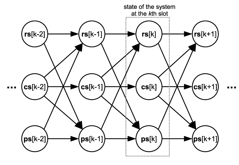

Fig. 2 depicts the dependence of the state variables over time. In this depiction, an arrow from variable to signifies that depends on . As shown in the figure, the ARQ state variables and depend on their previous values , , and also the previous channel state . For example, if transmits at ()th slot, ARQ state variables related to remain the same at the end of ()th slot: , and . The ARQ state variables related to alter depending on the channel states at slot : , and . Note that when a new round starts, the ARQ variables and are initialized to zero.
The flow chart of C-NC-ARQ is given in Fig. 2. As shown by this chart, the completion of a round depends on the condition that both packets from two source nodes are successfully decoded by the source nodes. (Packet from decoded at , packet from decoded at .) At the end of the transmission phase, if at least one packet fails, retransmission phase starts. Depending on the strategy, the retransmitting node and the retransmitted packet are chosen according to the C-NC-ARQ table which will be described in the sequel and the retransmissions are repeated until the successful round condition is satisfied. Three new retransmission strategies are proposed: relay-based retransmission with network coding, alternating retransmission with network coding, and channel state information based retransmission with network coding.
All three strategies are summarized in the C-NC-ARQ table in Table I. Each row of this table corresponds to an ARQ state shown in the left column. On the right column the corresponding retransmission rule is shown for the proposed methods. While the proposed methods utilize network coding, non-network-coded versions of the methods are also shown, for comparison. The retransmission rule is given by the notation , which represents the event that node transmits packet . For some of the rows, the transmitting node is . The node differs for the three different strategies, the mechanisms of which will be explained in the following.
| state at the beginning th slot | th slot | ||||
| with NC | without NC | ||||
III-A Relay-Based Retransmission with Network Coding Strategy (RR-NC)
According to the relay-based strategy, retransmissions are always executed by the relay if the relay has successfully received the packets to be retransmitted. Thus, in Table I. If the relay does not have the packets to be retransmitted, the retransmission is done by the original source node.
Note that network coding reduces the number of retransmissions by combining two unsuccessful packets for the case of , while the non-network coded method RR retransmits two packets at two individual slots. The relay-based strategy is expected to outperform when the fading margin of the relay channels are larger than the the fading margin of the direct channel.
III-B Alternating Retransmission with Network Coding Strategy (AR-NC)
The difference between AR-NC and RR-NC is that for repeated transmissions, the choice of retransmitting node alternates between the relay and the source node ( or ). As an example from Table I, when the case and occurs at the end of slot , retransmission is performed by the relay () at the th slot. If packet state does not change at the end of th slot ( and ), the source node is chosen as retransmitting node () for ()th slot. The alternating between the relay and the source continues for the rest of the retransmissions. The AR-NC strategy is a little more complex than the RR-NC strategy, since the former needs to keep track of the last retransmitting node. However, the AR-NC strategy is expected to improve upon RR-NC, especially for highly correlated block fading channels where the relay channel may enter into long duration outages.
III-C Channel State Information Based Retransmission with Network Coding Strategy (CR-NC)
Notice that at the beginning of slot , the nodes are aware of their channels and the channels of other nodes from the ACK/NAK feedback broadcasted in the previous slots. Using this information about the channel states in the previous slots, the choice of retransmitting node can be improved. For example, consider the case where and has occured, and the channel states at slot has been observed due to the ACK/NAK feedback. The retransmitting node is selected as the source () at the th slot if the direct channel was not in outage while relay channel was in outage at the ()th slot (, ). Otherwise the relay retransmits (). This strategy is expected to perform well for both slow and moderately fast fading since it exploits the previously observed channel states. Unless the channel fading very fast, the previous ACK/NAK observations will be good indicators of the channel states at slot .
IV Throughput Analysis
Throughput analysis of the C-NC-ARQ strategies are based on the states of the network. The three main states of the network are defined as (new round state), (new round-2 state), and (retransmission state). The schemes differ in how they behave when the network is in state. The defined network state is determined by the ARQ state variables , , and also the channel state . Since these state variables have the Markov dependence structure as shown in Fig. 2, the network state also has the Markov structure in time.

Let be the state of the C-NC-ARQ at the end of ()th slot, denotes that a round has been completed successfully at the end of ()th slot and a new round will start with transmitting at th slot. denotes that a round was completed successfully at ()th slot, a new round started at ()th slot, transmitted at ()th slot, and will transmit next, at th slot. After the new round-2 state , the system will either enter new round state if both packets are successful or enter retransmission state if at least one packet fails:
| (17) |
The transition of states are shown in Fig. 3 where represents the transition probability from state to state . For the finite- state Markov model in Fig. 3 with the states , and , state transition probability matrix is given below:
| (18) |
and steady-state probabilities are calculated from the equation below:
| (19) |
Since the state represents the new round state, whenever the system is in the state , it means that the packets and are successfully received by and , respectively. In steady-state, the ratio of expected number of successfully decoded packets to the total number of transmissions, which is defined as the average throughput, is equal to the steady-state probability of the state . Thus, average throughput is
| (20) |
We require the elements of the transition matrix to calculate the throughput. The elements of may differ depending on the strategies which are described in previous section.
In this contribution, our throughput analysis is based on the method in [7]. The variable , which represents the state of C-NC-ARQ, switches between the states , and depending on the packet state variables and , and channel state variable according to the Table I.
The state model of the C-NC-ARQ in Fig. 3 is helpful for representing the main operation of the system. However this model is a coarse representation which hides the channel state and ARQ state variables. All possible configurations of these variables are embedded in , , states of the model in Fig. 3. In order to help analyze the system, we define sub-states of , , , for different configurations of channel and ARQ state variables. The sub-states of the main system states , and are represented by the state vectors , and , respectively. All these sub-states in these vectors constitute a new Markov model, which will be represented by the variable .
The sub-states of the new round state are represented by the vector :
| (21) |
For slot , means that this slot is the first transmission slot of a new round, and the index is the channel state index for slot . This index is the decimal corresponding the the binary vector . For example, for a first transmission slot , refers to the sub-state .
The sub-states of the new round-2 state are for and , where the index is the decimal corresponding to , and is the channel state index for slot . The reason why need to be included in the sub-states is as follows: When the system is in state at the beginning of ()th slot, transmits at the ()th slot, so and preserve their previous values but and alter depending on the channel state variables and , respectively: , . The length- sub-state vector for is
| (22) |
The sub-states of the retransmission state depend on which transmission strategy is used. The relay-based retransmision strategy is the simplest one with the least number of sub-states. We will explain the sub-states of and the throughput analysis for the relay-based strategy first, and later describe how they differ for alternating and channel state information based methods.
For relay-based retransmission strategy, the sub-states of are
for and , where the index is the
decimal corresponding to binary vector
and
is again the channel state index at slot . Notice that the index has
values not larger than . This is because at the end of
the slot will prompt the start of a new round at slot . Let us next
investigate the transition probabilities between the defined sub-states.
IV-A Transition from Sub-states
From state at slot , there can only be transitions to , for , . This is because state is always followed by in the next slot. The channel state at slot completely determines whether packet transmitted by is received corectly by and at the end of slot , thus it completely determines and the index. Let us denote the index determined by the channel state index by . For the channel state index at the next slot, all values in are possible. Let us denote the probability of transitioning from channel state to channel state by . This probability is simply the product of the corresponding channels’ transitions, since , , channels are assumed to be independent. For example, transition from channel state to is
| (23) |
where , and were defined in Section II.
As a result, the transition probability from to is
| (24) |
IV-B Transition from Sub-states
From , there can be transitions to new round sub-states in or retransmission sub-states . A transition to indicates that the packets and were received successfully in the first attempt, without the assistance of retransmission, and a new round starts at slot . The indices and , (the states , and the channel state at slot ) determine whether the next state is . The next state is only if the following new round condition is met:
where the notation reads “ is such that ”. Thus the transition probability is
| (25) |
If the new round condition is not met, then the network enters a retransmission sub-state in the next slot: , where is the decimal value of
| (26) |
To simplify, we define the notation
| (27) |
The notation in (27) tells that, given state at slot is , we know the state , and the channel state at , from which we can find using (26), and the decimal conversion gives . Eq. (26) signifies that at the start of slot , packet and relay states for is the same as those at the start of slot , since was transmitted by at slot . Packet and relay states for are determined by the states of the channels and , respectively. So the transition probability is
| (28) |
IV-C Transition from Sub-states
It is possible to have or transitions. For , as opposed to the transitions from sub-states of and , the transmission at slot is not fixed but it depends on . For a given , the states and are given, which determine what will be transmitted at slot using the rule in Table I. Given the transmission rule and the channel state at , the next states and are found. If , then with probability , the system enters a new round, and is reset to zero. If , then with probability , where . As an example, we provide the list of transitions from for and in Table II. The index corresponds to , , and from Table I, we know that transmission will occur at slot for RR-NC strategy.
| Channel at slot | for | Transition probability | ||
|---|---|---|---|---|
IV-D Steady State Probabilities
In order to obtain the average throughput in (20), we need the steady state probabilities of the sub-states defined. To find the steady state distribution, we define the overall sub-state vector
| (29) |
The length of for the relay based retransmission strategy is . Next we construct the overall probability transition matrix . The th element of is:
| (30) |
The matrix is constructed using the sub-state transition probabilities explained in Subsections IV-A, IV-B, IV-C, and has the following structure:
| (31) |
The vector of steady state probabilities
| (32) |
is found from the solution of
Finally, the steady state probability of for the throughput in (20) is obtained as
| (33) |
IV-E Alternating and Channel State Information Based Retransmission Strategies
The throughput analyses for the alternating (AR-NC and AR) and channel state information based (CR-NC and CR) retransmission strategies are similar, except for the fact that the number of substates in increases.
For AR-NC and AR, we define a token index that alternates between and with each retransmission by in Table I. If then will retransmit, otherwise one of and will retransmit based on which packet is transmitted. The sub-states of are denoted by , and there are sub-states in the sub-state vector .
Similar to alternating retransmission strategies, there is a token variable that controls the retransmitting node for channel state information based retransmission strategies (CR-NC and CR). In this case, not all the sub-states include the token variable, just the rows in Table I which includes . For example, does not include token variable whereas does. According to the state , retransmission is realized by relay if else retransmits. Unlike the operation in AR-NC or AR, token variable is not altered after every transmission because retransmitting node is selected according to the previous channel state variable . So, the number of sub-states in is for CR-NC, and for CR.
V Numerical Results
In this section we provide performance results of C-NC-ARQ methods for different channel conditions, and observe the effect of channel correlation on the network throughput performance. The simulation results are obtained using Monte Carlo simulations where fading channels are randomly generated using (5) and the protocol rules given in Table I.
In Fig. 4, network throughput performance of RR-NC and RR can be seen for different correlation coefficients. Three different correlation coefficients are examined: uncorrelated (), highly correlated (), fully correlated () cases. Analytical results are compared with the Monte-Carlo simulalation results, and it is observed that analytical and simulation results coincide. The case where the fading margins of relay channels are higher than that of direct channel is considered: dB where for . As a comparison, the throughput of conventional stop-and-wait ARQ is also shown, which is . It is observed that for large values of outage probability (for ), the channel correlation has a negative impact on the throughput performance. This is due to the cases where the retransmission phase is locked in repeated relay retransmission, whose channel is in a long-duration outage. Such a threshold for can be defined as for the case where dB. For and , we observe the positive impact of channel correlation. This is explained by low probability of outage combined with the diversity advantage of the relay mean that highly correlated block fading channels result in long-duration good state channels. Another important observation is that network coding can improve throughput by , which is a significant improvement.
Similar behaviors are observed for the alternating retransmission strategy in Fig. 5 and channel state information based retransmission strategy in Fig. 6.


The three retransmission strategies are compared in Fig.7. In this figure, only analytically obtained throughput results are shown. Fully correlated case of the channel is investigated in Fig.7, as a function of the fading margin, where the relay channels have the same fading margins as the direct channel, dB. For the case of high correlation, , the relay based retransmission strategy performs worse than AR, CR and even traditional ARQ, especially for low fading margin. This is due to the fact that RR strategy repeatedly attempts to retransmit from consequtive bad relay channels. For the AR and CR strategies, this situation does not occur.

In Fig. 8, the throughput performances are shown as a function of the correlation coefficient for fixed dB and the cases where the relay channels have better fading margins than the direct channel ( dB), and where the relay channels have the same fading margins as the direct channel. For the case when the relay channels have good average reliability ( dB), we observe the gain due to the network coding for all three strategies whereas for the dB case the improvement is not so significant. This is due to the fact that, in order to see the network coding advantage the ARQ state , in Table I needs to occur frequently, which happens when the relay channels are better than the direct channel on average. For the dB case, the relay based retransmission strategy outperforms the alternating retransmission strategy because the relay channels are better than the direct channel on average and alternating between relay and source degrades performance for this case. It is observed that unless the channel correlation is ver low, the channel state information based strategy performs best among the three strategies. For channel correlation close to zero, the channel state of the previous slot provides no information about the current slot so the choice of the channel state information based strategy becomes almost arbitrary. For the dB case, the relay based retransmission strategy performs worst because it insists on repeated transmissions from the relay eventhough the relay channel may not be in a good state for repeated slots, especially for large values of channel correlation.

The performances are shown as a function of the relay fading margin in Fig. 9. As expected, the relay based retransmission strategy is poor for low values of relay channel fading margin. For large values of , the relay based retransmission strategy works well, slightly better than the channel state information based retransmission for , and slightly worse than the channel state information based retransmission for . It is observed that for the case where the relay channel is worse than the direct channel ( dB) and very low correlation values (), cooperative ARQ strategies may actually perform worse than the traditional ARQ. When the relay channel is much better than the direct channel ( dB) relay based retransmission can be a good choice, otherwise alternating and channel state information based strategies work well.


Finally, we note that in the analysis of the channel state information based retransmission strategy, it was assumed that the channel state information of the previous slot (()th slot) is available for deciding the transmission at slot . The channel state information is going to be obtained utilizing the ACK/NAK feedback at each slot. However, the ACK/NAK feedback of all chanels may not be available for the previous slot. In practice, the latest received ACK/NAK feedback is going to be used as the last known state of each channel, which may degrade the performance since the channel state information may be outdated. In order to investigate this effect, we provide Fig. 10, where the channel state information based retransmission strategy using channel state information of previous slot and the last known slot are compared. For comparison, we also show the performance of the case where the channel state information of the current slot is utilized. It is observed that the throughput performances are very close.
VI Conclusion
In this paper, novel cooperative ARQ methods which integrate network coding into retransmission phase are proposed and performance of the proposed methods are analyzed for two-way relay network. An analytical method is derived for obtaining network throughput for correlated channels and is utilized to compare different cooperative ARQ methods for different channel settings. It is observed that unless the average outage rate of the relay channels are worse than the direct channel and the channel is very fast fading, the proposed strategies improve performance. The impact of network coding is seen when the relay channels have a fading margin of dB or larger. Channel correlation in time improves the gain of the proposed methods in general. Among the proposed retransmission strategies, relay based retransmission is the simplest one, and can be a good choice if the average reliability of the relay channel is good. The channel state information based retransmissionis the best strategy if the nodes can keep track of the last known channel state information.
The generalization of the methods and their analyses to a more general network model with more relays and sources remains as a future work.
References
- [1] E. C. van der Meulen, “Three-terminal communication channel,” Advanced Applied Probability, vol. 3, pp. 120–154, 1971.
- [2] T. M. Cover and A. A. El Gamal, “Capacity theorems for the relay channel,” IEEE Trans. Inf. Theory, vol. 52, no. 5, pp. 572–584, Sep. 1979.
- [3] A. Sendonaris, E. Erkip, and B. Aazhang, “User cooperation diversity-Part I: System description,” IEEE Trans. Commun., vol. 51, no. 11, pp. 1927–1938, Nov. 2003.
- [4] J. N. Laneman, D. N. C. Tse, and G. W. Wornell, “Cooperative diversity in wireless networks: Efficient protocols and outage behavior,” IEEE Trans. Inf. Theory, vol. 50, no. 12, pp. 3062–3080, Dec. 2004.
- [5] A. Nosratinia, T. E. Hunter, and A. Hedayat, “Cooperative communication in wireless networks,” IEEE Commun. Mag., vol. 42, no. 10, pp. 74–80, Oct. 2004.
- [6] B. Zhao and M. C. Valenti, “Practical relay networks: A generalization of hybrid-ARQ,” IEEE J. Sel. Areas Commun., vol. 23, no. 1, pp. 7–18, Jan. 2005.
- [7] M. Dianati, X. Ling, K. Naik, and X. Shen, “A node-cooperative ARQ scheme for wireless ad hoc networks,” IEEE Trans. Veh. Technol., vol. 55, no. 3, pp. 1032–1044, May 2006.
- [8] G. Yu, Z. Zhang, and P. Qiu, “Cooperative ARQ in wireless networks: Protocols description and performance analysis,” in IEEE International Conference on Communications, ICC, 11-15 June 2006, pp. 3608–3614.
- [9] I. Stanojev, O. Simeone, Y. Bar-Ness, and C. You, “Performance of multi-relay collaborative hybrid-ARQ protocols over fading channels,” IEEE Commun. Lett., vol. 10, no. 7, pp. 522–524, Jul. 2006.
- [10] I. Byun and K. S. Kim, “Cooperative hybrid-ARQ protocols: Unified frameworks for protocol analysis,” ETRI Journal, vol. 33, no. 5, pp. 759–769, Oct. 2011.
- [11] R. Ahlswede, N. Cai, S.-Y. R. Li, and R. W. Yeung, “Network information flow,” IEEE Trans. Inf. Theory, vol. 46, no. 4, pp. 1204–1216, Jul. 2000.
- [12] S. R. Li, R. W. Yeung, and C. Ning, “Linear network coding,” IEEE Trans. Inf. Theory, vol. 49, no. 2, pp. 371–381, Feb. 2003.
- [13] R. Koetter and M. Medard, “An algebraic approach to network coding,” IEEE/ACM Trans. Netw., vol. 11, no. 5, pp. 782–795, Oct. 2003.
- [14] S. Zhang, S. C. Liew, and P. P. Lam, “Hot topic: Physical-layer network coding,” in 12th Annual International Conference on Mobile Computing and Networking, MOBICOM, 24-29 September 2006, pp. 358–365.
- [15] S. Katti, H. Rahul, H. Wenjun, D. Katabi, M. Medard, and J. Crowcroft, “XORs in the air: Practical wireless network coding,” IEEE/ACM Trans. Netw., vol. 16, no. 3, pp. 497–510, Jun. 2008.
- [16] R. H. Y. Louie, Y. Li, and B. Vucetic, “Practical physical layer network coding for two-way relay channels: performance analysis and comparison,” IEEE Trans. Wireless Commun., vol. 9, no. 2, pp. 764–777, Feb. 2010.
- [17] J. K. Sundararajan, D. Shah, and M. Medard, “ARQ for network coding,” in IEEE International Symposium on Information Theory, ISIT, 6-11 July 2008, pp. 1651–1655.
- [18] T. Tran, T. Nguyen, B. Bose, and V. Gopal, “A hybrid network coding technique for single-hop wireless networks,” IEEE J. Sel. Areas Commun., vol. 27, no. 5, pp. 685–698, Jun. 2009.
- [19] D. Nguyen, T. Tran, T. Nguyen, and B. Bose, “Wireless broadcast using network coding,” IEEE Trans. Veh. Technol., vol. 58, no. 2, pp. 914–925, Feb. 2009.
- [20] S. Sorour and S. Valaee, “An adaptive network coded retransmission scheme for single-hop wireless multicast broadcast services,” IEEE/ACM Trans. Netw., vol. 19, no. 3, pp. 869–878, Jun. 2011.
- [21] Q.-T. Vien, L.-N. Tran, and H. X. Nguyen, “Network coding-based ARQ retransmission strategies for two-way wireless relay networks,” in International Conference on Software, Telecommunications and Computer Networks, SoftCOM, 23-25 September 2010, pp. 180–184.
- [22] P. Fan, C. Zhi, C. Wei, and K. B. Letaief, “Reliable relay assisted wireless multicast using network coding,” IEEE J. Sel. Areas Commun., vol. 27, no. 5, pp. 749–762, Jun. 2009.
- [23] Q.-T. Vien, L.-N. Tran, and E.-K. Hong, “Network coding-based retransmission for relay aided multisource multicast networks,” EURASIP Journal on Wireless Communications and Networking, vol. 2011:643920, 2011.
- [24] S. Qi, L. Yonghua, H. Zhiqiang, and L. Jiaru, “On reliable multicast with network coding-ARQ for relay cooperation cells,” in IEEE 75th Vehicular Technology Conference, Spring, VTC, 6-9 May 2012, pp. 1–5.
- [25] A. Munari, F. Rossetto, and M. Zorzi, “Phoenix: Making cooperation more efficient through network coding in wireless networks,” IEEE Trans. Wireless Commun., vol. 8, no. 10, pp. 5248–5258, Oct. 2009.
- [26] X. Shi, J. Ge, Y. Ji, and C. Sun, “Network-coding-based hybrid ARQ for two-way relaying,” in Fourth International Conference on Intelligent Networking and Collaborative Systems, 19-21 September 2012, pp. 536–540.
- [27] A. Antonopoulos, C. Verikoukis, C. Skianis, and O. B. Akan, “Energy efficient network-coding based MAC for cooperative ARQ wireless networks,” Ad Hoc Networks, vol. 11, pp. 190–200, 2013.
- [28] H. S. Wang and N. Moayeri, “Finite-state Markov channel – a useful model for radio communication channels,” IEEE Trans. Veh. Technol., vol. 44, no. 1, pp. 163–171, Feb. 1995.
- [29] M. Zorzi, R. R. Rao, and L. B. Milstein, “Error statistics in data transmission over fading channels,” IEEE Trans. Commun., vol. 46, no. 11, pp. 1468–1477, Nov. 1998.
- [30] Q. Zhang and S. A. Kassam, “Finite-state Markov model for Rayleigh-fading channels,” IEEE Trans. Commun., vol. 47, no. 11, pp. 1688–1692, Nov. 1999.
- [31] F. Babich and G. Lombardi, “A Markov model for the mobile propagation channel,” IEEE Trans. Veh. Technol., vol. 49, no. 1, pp. 63–73, Jan. 2000.
- [32] E. N. Gilbert, “Capacity of a burst-noise channel,” Bell System Technical Journal, vol. 39, pp. 1253–1265, 1960.
- [33] E. O. Elliot, “Estimates of error rates for codes on burst-noise channels,” Bell System Technical Journal, vol. 42, pp. 1977–1997, 1963.
- [34] M. Zorzi, R. R. Rao, and L. B. Milstein, “ARQ error control for fading mobile radio channels,” IEEE Trans. Veh. Technol., vol. 46, no. 2, pp. 445–455, May 1997.
- [35] C. Pimentel, T. H. Falk, and L. Lisboa, “Finite-state Markov modeling of correlated Rician-fading channels,” IEEE Trans. Veh. Technol., vol. 53, no. 5, pp. 1491–1501, Sep. 2004.
- [36] H. Kong and E. Shwedyk, “A hidden Markov model (HMM)-based MAP receiver for Nakagami fading channels,” in IEEE International Symposium on Information Theory, ISIT, 17-22 September 1995, p. 210.
- [37] G. Caire, G. Taricco, and E. Biglieri, “Optimum power control over fading channels,” IEEE Trans. Inf. Theory, vol. 45, no. 5, pp. 1468–1489, Jul. 1999.
- [38] E. Malkamaki and H. Leib, “Coded diversity on block-fading channels,” IEEE Trans. Inf. Theory, vol. 45, no. 2, pp. 771–781, Mar. 1999.
- [39] A. G. i Fabregas and G. Caire, “Coded modulation in the block-fading channel: coding theorems and code construction,” IEEE Trans. Inf. Theory, vol. 52, no. 1, pp. 91–114, Jan. 2006.
- [40] D. Tse and P. Viswanath, Fundamentals of Wireless Communication. New York: Cambridge University Press, 2005.