Fitting Voronoi Diagrams to Planar TesselationsThanks: Mathematics Subject Classification: 52C45, 65D18, 68U05.
Abstract
Given a tesselation of the plane, defined by a planar straight-line graph , we want to find a minimal set of points in the plane, such that the Voronoi diagram associated with ‘fits’ . This is the Generalized Inverse Voronoi Problem (GIVP), defined in [12] and rediscovered recently in [3]. Here we give an algorithm that solves this problem with a number of points that is linear in the size of , assuming that the smallest angle in is constant.
Keywords:
Voronoi diagram, Dirichlet tesselation, planar tesselation, inverse Voronoi problem1 Introduction
Any planar straight-line graph (PSLG) subdivides the plane into cells, some of which may be unbounded. The Voronoi diagram (also commonly referred to as Dirichlet tesselation, or Thiessen polygon) of a set of points is a PSLG with cells, where each cell belongs to one point from and consists of all points in the plane that are closer to that point than to any other in .
Let be a given PSLG, whose cells can be considered bounded and convex for all practical purposes. Indeed, if some cell is not convex, it can always be partitioned into convex subcells, thus yielding a finer tesselation. The asymptotic size complexity of the PSLG remains the same by this ‘convexification’ operation.
The Inverse Voronoi Problem (IVP) consists of deciding whether coincides with the Voronoi diagram of some set of points in the plane, and if so, finding . This problem was first studied by Ash and Bolker [1]. Subsequently, Aurenhammer presented a more efficient algorithm [2], which in turn was improved by Hartvigsen, with the aid of linear programming [5], and later by Schoenberg, Ferguson and Li [8]. Yeganova also used linear programming to determine the location of [13, 14].
In the IVP, the set is limited to have one point per cell; a generalized version of this problem (GIVP) allows more than one point per cell. In this case, new vertices and edges may be added to , but the original ones must be kept, as shown in Figure 1. With this relaxation the set always exists, hence we are interested in minimizing its size.

The GIVP in was indirectly mentioned in [13, 14], in the context of set separation. It was formally stated and discussed in the III Cuban Workshop on Algorithms and Data Structures, held in Havana in 2003, where an algorithm for solving the problem in was sketched by the current authors. However, the manuscript remained dormant for several years, and the algorithm was only published in Spanish in 2007 [12]. Recently, the problem was revisited in [3], where another algorithm for the GIVP in is given, and the special case of a rectangular tesselation is discussed in greater detail. The authors of [3] were unaware of [12], however the two algorithms turn out to have certain common aspects.
This paper is an expanded and updated English version of [12]. It contains a description and analysis of the aforementioned algorithm for solving the GIVP in . This is followed by the description of an implementation of the algorithm, which was used to make a first (if only preliminary) experimental study of the algorithm’s performance. Our algorithm generates sites in the worst case, where is the number of edges of (provided that the smallest angle of is constant). This bound is asymptotically optimal for tesselations with such angular constraints.
In comparison, the analysis given for the algorithm in [3] states that sites are generated, where is the size of a refinement of such that all faces are triangles with acute angles. Given an arbitrary PSLG, there does not appear to be any known polynomial upper bound on the size of its associated acute triangulation. Even though it seems to us that the analysis in [3] should have given a tighter upper bound in terms of , even a linear bound would not make much of a difference, given that can be very large compared to the size of . The analysis in [3] is purely theoretical, so it would be interesting to perform an experimental study to shed some light on the algorithm’s performance in practice.
This paper is organized as follows: In Section 2 we describe the algorithm and discuss its correctness and performance. In Section 3 we derive some variants of the general strategy, and deal with several implementation issues of each variant. Section 4 is devoted to an experimental analysis of the algorithm’s performance. Finally, in Section 5 we summarize our results and discuss some open problems arising as a result of our work.
2 The Algorithm
First we establish some notation and definitions. In that respect we have followed some standard texts, such as [4].
Let and be points of the plane; as customary, is the segment that joins and , and denotes its length. denotes the bisector of and , and is the half-plane determined by , containing . For a set of points in the plane, Vor() denotes the Voronoi diagram generated by . The points in are called Voronoi sites or generators.
If , denotes the cell of Vor() corresponding to the site . For any point , is the largest empty circle centered at , with respect to (the subscript can be dropped if it is clear from the context). Two points are said to be (strong) neighbors (with respect to ) if their cells share an edge in Vor(); in this case denotes that edge.
We will make frequent use of the following basic property of Voronoi diagrams:
Lemma 1 ([4], Thm. 7.4, p. 150)
The bisector defines an edge of the Voronoi diagram if, and only if, there exists a point on such that contains both and on its boundary, but no other site. The (open) edge in question consists of all points with that property.
The technique used by the algorithm is to place pairs of points (sentinels) along each edge of the PSLG (each pair is placed so that it is bisected by ) in order to ‘guard’ or ‘protect’ . The number of sentinels required to protect depends on its length and the relative positions of its neighboring edges. Each pair of sentinels meant to guard is placed on the boundary of some circle, whose center lies on . Furthermore this circle will not touch any other edge. The only exception is when the circle is centered on an endpoint of , in which case it is allowed to touch all other edges sharing that endpoint. More formally, we have the following.
Definition 1
Let be a PSLG, and let be an edge of . Let be a set of points, and . The pair of points is said to be a pair of sentinels of if they are strong neighbors with respect to , and is a subsegment of . In this case, (or more precisely, the segment ) is said to be guarded by and .
The algorithm works in two stages: First, for each vertex of we draw a circle centered on . This is our set of initial circles (this is described in more detail below). Then we proceed to cover each edge of by non-overlapping inner circles, whose centers lie on , and which do not intersect any other edges of .
Let be a given vertex of , and let be the length of the shortest edge of incident to . We denote as the initial circle centered at , which will be taken as the largest circle with radius that does not intersect any edge of , except those that are incident to . Once we have drawn , for each edge incident to we can choose a pair of sentinels , placed on , one on each side of , at a suitably small distance from , as in Figure 2. Later in this section we discuss how to choose appropriately.
Let be the point of intersection between and ; now and guard the segment of , which means that will appear in the Voronoi diagram that will be constructed, provided that we do not include any new points inside (see Lemma 1).
Let be an edge of , and the intersection points of and with , respectively.11 1 For convenience, we have dropped the subscript . The segments and are now guarded, whereas the (possibly empty) segment still remains unguarded. In order to guard it suffices to cover that segment with circles centered on it, not intersecting with any edge other than , and not including any sentinel belonging to another circle. Then we can choose pairs of sentinels on each covering circle, each sentinel being at distance from , as shown in Figure 3.
As a consequence of Lemma 1, will be guarded in all its length, provided that no new point is later included inside one of the circles centered on . To ensure this, we will not allow an inner circle of to get closer than to another edge , because then a sentinel of might fall inside the circle. With this precaution, the sentinels guarding will not interfere with other edges, since they will not be included in any circle belonging to another edge.
In summary, an outline of the algorithm is:
- 1.
For each vertex , draw initial circle centered on .
- 2.
Choose a suitable value of .
- 3.
For each vertex and for each edge incident to , place a pair of sentinels on , symmetric to one another with respect to , at distance from .
- 4.
For each edge , cover the unguarded segment of with inner circles centered on , and then place pairs of sentinels on each circle.
This algorithm is a general strategy that leads to several variants when Step 4 is specified in more detail, as will be seen in Section 3. In order to prove that the algorithm works it suffices to show that:
- 1.
The algorithm terminates after constructing a finite number of circles (and sentinels).
- 2.
After termination, every edge of is guarded (see the discussion above).
In order to show that the algorithm terminates we will establish some facts. Let be the radius of the smallest initial circle. Now let be the smallest angle formed by any two incident edges of , say and . By taking we make sure that any sentinel will be closer to the edge that it is meant to guard than to any other edge. This is valid for all initial circles.
After all initial circles have been constructed, together with their corresponding sets of sentinels, for every edge there may be a middle segment that remains unguarded. This segment must be covered by a finite number of inner circles. Take one edge, say , with middle unguarded segment of length . If we use circles of radius to cover the unguarded segment, then we can be sure that these circles will not intersect any circle belonging to another edge. Exactly such circles will suffice to cover the middle segment, where the last one may have a radius smaller than . For this last circle, the sentinels could be placed at distance from (c.f. Figure 4).
Using circles of radius is, among all the possible variants mentioned here, the one that yields the largest number of circles, and hence the largest number of sentinels (generators of the Voronoi diagram). Now let be the longest edge of , with length . In the worst case, the number of inner circles that cover will be , and the number of sentinels will be twice that number plus four (corresponding to the sentinels of both initial circles). Therefore, the algorithm generates a number of points that is linear in , the number of edges, which is asymptotically optimal, since a lower bound for the number of points is the number of faces in .
Note that by letting become part of the problem instance, the number of generators becomes a function of , and it is no longer linear in . In practice, however, screen resolution and computer arithmetic impose lower bounds on . Under such constraints, the above analysis remains valid. This leads to our main result:
Theorem 2.1
Let be a planar straight-line graph, whose smallest angle is larger than a fixed constant. Then, the corresponding Generalized Inverse Voronoi Problem can be solved with generators, where is the number of edges of .
3 Implementation
In step 4 of the algorithm given in the previous section, the method to construct the inner circles was left unspecified. Taking the circles with radius , as suggested in the preceding analysis, is essentially a brute-force approach, and may easily result in too many sentinels being used. In this section we discuss two different methods for constructing the inner circles.
First let us note that in order to reduce the number of sentinels in our construction we may allow two adjacent circles on the same edge to overlap a little, so that they can share a pair of sentinels (see Figure 5). This observation is valid for all variants of the algorithm.
The first variant for the construction of the inner circles along an edge is to place them sequentially (iteratively), letting them grow as much as possible, provided that they do not enter the -wide ‘security area’ of another edge. Obviously, this greedy heuristic must yield a smaller number of Voronoi generators than the naive approach of taking all circles with radius .
Suppose we want to construct an inner circle for edge , adjacent to another circle on that has already been fixed and on which we have already placed two sentinels: , and . Let be the first edge that will be touched by as it grows, while constrained to have its center on and on its boundary. Let be a straight line parallel to , at distance from , and closer to than . Let be defined by the equation , and by the equation .22 2 The equation of can be obtained easily after the initial circles have been constructed and their sentinels placed. The distance of any point to is given by . The radius of must be equal to this distance. Hence the -coordinate of the center satisfies the following quadratic equation:
or
where .
Our second variant for constructing inner circles is also based on the principle of letting them grow until they come within distance of some edge. Yet, instead of growing the circles sequentially along the edge that is to be covered, we center the first inner circle on the midpoint of the unguarded middle segment. This will yield at most two smaller disjoint unguarded segments, on which we recurse. In the worst case, a branch of the recursion will end when an unguarded segment can be covered by a circle of radius .
The advantage of this approach is that the coordinates of the center can be determined with much less computation, thus avoiding potential roundoff errors. Additionally, this variant is more suitable for parallel implementation than the previous one. On the other hand, we need an extra data structure to handle the unguarded segments.
We end this discussion with a word about the choice of . On one hand, must be sufficiently small for the construction to be carried out. On the other hand, for the sake of robustness to numerical errors, it is convenient to take as large as possible. That is why we defer the actual choice of until the initial circles have been drawn. A different approach might be to use a variable-sized , which would lead to a more complicated, yet (hopefully) more robust algorithm.
A final remark: For the sake of simplicity we have assumed throughout the whole discussion that the cells of the input tesselation are convex, but our algorithm could be easily generalized to accept tesselations with non-convex cells.
4 Experimental Analysis
From the analysis in Section 2 we know that the number of sites generated by our algorithm is linear in the size of the input, provided that the smallest angle is constant. However, we would like to get a more precise idea about the algorithm’s performance, and the difference between the two strategies we have suggested for Step 4. For that purpose, we have implemented the algorithm and carried out a set of experiments.
Our experimental workbench consists of a Graphical User Interface, which can generate a tesselation on a random point set, store it in a DCEL data structure, and then apply one of the two variants of the algorithm for solving the GIVP, described in Section 2.
The GUI is described in more detail in [11, 12], and a beta Windows version can be downloaded from https://www.researchgate.net/publication/239994361_Voronoi_data. The file ‘Voronoi data.rar’ contains the Windows executable and a few DCEL files, consisting of sample tesselations. The user can generate additional tesselations randomly, and apply either variant of the algorithm on them.
The tesselations are generated as follows: First, the vertex set of is randomly generated from the uniform distribution in a rectangular region. Then, pairs of vertices are chosen randomly to create edges. If a new edge intersects existing edges, then the intersection points are added as new vertices, and the intersecting edges are decomposed into their non-intersecting segments. Finally, some edges are added to connect disjoint connected components and dangling vertices, so as to make the PSLG biconnected.
Table 1 displays some statistics about 40 such randomly generated tesselations: Number of vertices, number of edges, number of regions, number of Voronoi sites with the recursive version of Step 4, number of Voronoi sites with the sequential version of Step 4, the smallest angle , and the width of the security area. The tesselations have been listed in increasing order of the number of edges. For each parameter, the table also provides the median (MED), the mean value (AVG), and the standard deviation (STD).
| Num. of sites generated | |||||||
| Exp. | Tesselation | Smallest | |||||
| num. | Recursive | Sequential | angle | -neigh. | |||
| Vertices | Edges | Regions | version | version | (degrees) | (pixels) | |
| 1 | 72 | 142 | 66 | 1 020 | 852 | 1.63 | 1.20 |
| 2 | 117 | 206 | 91 | 916 | 870 | 4.09 | 12.30 |
| 3 | 194 | 252 | 60 | 1 468 | 1 296 | 1.07 | 9.61 |
| 4 | 274 | 376 | 105 | 1 672 | 1 596 | 1.60 | 12.26 |
| 5 | 229 | 429 | 202 | 2 400 | 2 148 | 3.38 | 0.91 |
| 6 | 314 | 441 | 129 | 2 208 | 2 020 | 0.56 | 5.70 |
| 7 | 336 | 472 | 138 | 2 656 | 2 374 | 0.47 | 4.03 |
| 8 | 339 | 475 | 138 | 3 098 | 2 618 | 3.95 | 0.18 |
| 9 | 344 | 480 | 138 | 3 140 | 2 720 | 0.23 | 4.48 |
| 10 | 357 | 493 | 138 | 2 844 | 2 530 | 0.13 | 7.24 |
| 11 | 339 | 501 | 164 | 2 580 | 2 364 | 0.38 | 3.81 |
| 12 | 390 | 568 | 180 | 2 680 | 2 520 | 8.92 | 0.60 |
| 13 | 438 | 637 | 281 | 3 320 | 3 028 | 0.21 | 6.34 |
| 14 | 403 | 641 | 240 | 3 838 | 3 382 | 0.16 | 7.07 |
| 15 | 472 | 684 | 214 | 3 432 | 3 144 | 0.25 | 2.56 |
| 16 | 397 | 721 | 319 | 4 244 | 3 718 | 0.11 | 3.16 |
| 17 | 421 | 784 | 365 | 5 112 | 4 406 | 1.30 | 0.12 |
| 18 | 564 | 826 | 264 | 4 092 | 3 790 | 0.70 | 0.11 |
| 19 | 504 | 986 | 463 | 4 148 | 4 020 | 2.37 | 14.16 |
| 20 | 512 | 999 | 472 | 4 276 | 4 134 | 1.52 | 3.68 |
| 21 | 552 | 1 056 | 506 | 4 048 | 4 796 | 0.25 | 4.40 |
| 22 | 574 | 1 107 | 535 | 4 856 | 4 689 | 3.68 | 0.75 |
| 23 | 601 | 1 166 | 567 | 5 240 | 5 009 | 0.80 | 3.43 |
| 24 | 645 | 1 256 | 613 | 5 852 | 5 521 | 0.77 | 3.62 |
| 25 | 672 | 1 292 | 622 | 5 720 | 5 992 | 0.25 | 3.44 |
| 26 | 738 | 1 311 | 575 | 6 124 | 5 832 | 0.34 | 1.84 |
| 27 | 724 | 1 399 | 677 | 6 440 | 6 194 | 0.23 | 3.23 |
| 28 | 815 | 1 441 | 628 | 6 832 | 6 478 | 1.20 | 0.30 |
| 29 | 763 | 1 479 | 718 | 6 960 | 6 599 | 2.14 | 0.19 |
| 30 | 772 | 1 495 | 725 | 6 900 | 6 610 | 2.54 | 0.29 |
| 31 | 855 | 1 522 | 669 | 7 684 | 7 158 | 1.43 | 0.31 |
| 32 | 894 | 1 607 | 712 | 9 062 | 8 685 | 0.36 | 0.23 |
| 33 | 898 | 1 615 | 716 | 8 152 | 7 580 | 1.19 | 0.33 |
| 34 | 963 | 1 750 | 789 | 9 637 | 9 045 | 0.88 | 0.29 |
| 35 | 1 006 | 1 842 | 838 | 9 236 | 8 582 | 1.85 | 0.34 |
| 36 | 1 018 | 1 874 | 858 | 10 144 | 9 228 | 1.09 | 0.27 |
| 37 | 984 | 1 902 | 920 | 7 924 | 7 792 | 4.40 | 0.25 |
| 38 | 1 015 | 1 962 | 949 | 8 396 | 8 198 | 3.34 | 0.31 |
| 39 | 1 066 | 1 973 | 909 | 10 392 | 9 492 | 0.63 | 0.30 |
| 40 | 1 019 | 1 999 | 982 | 8 952 | 8 616 | 1.49 | 0.45 |
| MED | 558 | 1 027.5 | 489 | 4 566 | 4 547.5 | 3.4 | 0.3 |
| AVG | 590 | 1 054 | 467 | 5 192 | 4 891 | 0.59 | 4.06 |
| STD | 282.7 | 571.24 | 292.73 | 2 715.5 | 2 600 | 3.36 | 0.74 |
From the tabulated data we can also get empirical estimates about the correlation among different parameters, especially and , and about the distribution of their values. The parameters and show a weak negative correlation with the number of edges, of and respectively. In turn they are positively correlated with one another, with a correlation of . These empirical findings agree with intuition.
Figures 7 and 7 display the histograms of and with 20 bins. They can be well approximated by Poisson distributions, with and , respectively, and with 95% confidence intervals and .


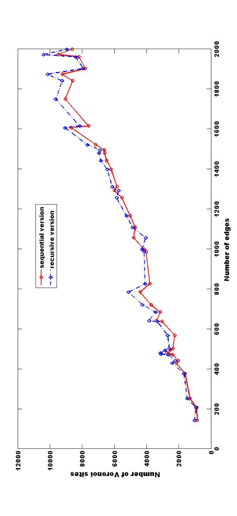
The comparison between the two variants of the algorithm is shown in Figure 8. We can see that the sequential variant is slightly better than the recursive variant, as it generates a smaller number of sites in most cases. However, the difference between both variants is not significant. Indeed, the linear regression fits have very similar slopes: The linear fit for the sequential variant is , whereas the linear fit in the recursive case is .
5 Conclusions and Open Problems
Our results show that the Generalized Inverse Voronoi Problem can be solved with a number of generators that is linear in the size of the input tesselation, provided that we enforce a lower bound on the size of the smallest angle. On the other hand, the algorithm described in [3] produces generators, where is the number of vertices of an acute triangulation of . As the performance of the two algorithms is given as a function of different parameters, a theoretical comparison between them is not straightforward. An experimental study could be helpful, but that would require an implementation of the algorithm in [3]. In practice, our algorithm generates approximately Voronoi sites, where is the number of edges of the input tesselation.
In any case, the number of generators produced by both algorithms may still be too large, and it may be possible to reduce it to a number closer to , the number of faces of the tesselation, which is the trivial lower bound. This lower bound can only be achieved if the tesselation is a Voronoi tesselation. In the more general case, how close to can we get?
In particular, our algorithm still has plenty of room for improvement. In Section 3 we have already mentioned several strategies that can decrease the number of Voronoi sites produced. The design of a parallel version, and a version that is robust against degenerate cases and numerical roundoff errors, are other issues to consider. Roundoff errors have long been an important concern in Computational Geometry in general, and in Voronoi diagram computation, in particular (see e.g. [10]).
Other practical questions have to do with the experimental analysis of our algorithms. We have devised a method to generate a PSLG on a random point set, but we have not analyzed how this compares to generating such graphs uniformly from the set of all PSLGs that can be defined on a given point set. Regarding certain properties of our generated graphs (expected number of vertices, edges, and faces, expected area of the faces, distribution of the smallest angle, etc.), we have not attempted a theoretical analysis, but we have estimated some of these parameters empirically. A more comprehensive set of experiments will reveal how these tesselations compare with those generated by other methods.
As a final remark, we point out that our algorithm could also be generalized to other metrics, continuous or discrete, including graph metrics. Potential applications include image representation and compression, as described in [6], and pattern recognition (e.g. given a partition of some sample space, we could select a set of ‘representatives’ for each class). In the case of graphs, Voronoi partitions can be used to find approximate shortest paths (see [9, 7], for instance). In social networks, node clustering around a set of ‘representative’ nodes, or ‘super-vertices’, is a popular technique for network visualization andor anonymization [15].
Acknowledgements
Janos Pach contributed some key ideas for the algorithm, at the early stages of this work. Hebert Pérez-Rosés was partially supported by the Spanish Ministry of Economy and Competitiveness, under project TIN2010-18978. Guillermo Pineda-Villavicencio was supported by a postdoctoral fellowship funded by the Skirball Foundation, via the Center for Advanced Studies in Mathematics at the Ben-Gurion University of the Negev, Israel, and by an ISF grant.
References
- [1] Ash, P., Bolker, E.D. Recognizing Dirichlet Tesselations. Geometriae Dedicata 19, 175–206 (1985).
- [2] Aurenhammer, F. Recognising Polytopical Cell Complexes and Constructing Projection Polyhedra. J. Symbolic Computation 3, 249–255 (1987).
- [3] Banerjee, S., Bhattacharya, B.B., Das, S., Karmakar, A., Maheshwari, A., Roy, S. On the Construction of a Generalized Voronoi Inverse of a Rectangular Tesselation. In: Procs. 9th Int. IEEE Symp. on Voronoi Diagrams in Science and Engineering, pp. 132–137. IEEE, New Brunswick, NJ (2012).
- [4] de Berg, M., Cheong, O., van Kreveld, M., Overmars, M.: Computational Geometry. Algorithms and Applications. Springer, Berlin, third ed. (2008).
- [5] Hartvigsen, D. Recognizing Voronoi Diagrams with Linear Programming. ORSA J. Comput. 4, 369–374 (1992).
- [6] Martínez, A., Martínez, J., Pérez-Rosés, H., Quirós, R. Image Processing using Voronoi diagrams. In: Procs. 2007 Int. Conf. on Image Proc., Comp. Vision, and Pat. Rec., pp 485-491. CSREA Press (2007).
- [7] Ratti, B., Sommer, C. Approximating Shortest Paths in Spatial Social Networks. In: Procs. 2012 ASE/IEEE Int. Conf. on Social Computing and 2012 ASE/IEEE Int. Conf. on Privacy, Security, Risk and Trust, pp 585–586. IEEE Comp. Soc. (2012).
- [8] Schoenberg, F.P., Ferguson, T., Li, C. Inverting Dirichlet Tesselations. The Computer J. 46, 76–83 (2003).
- [9] Sommer, C.: Approximate Shortest Path and Distance Queries in Networks. PhD Thesis, Department of Computer Science, The University of Tokyo, Japan (2010).
- [10] Sugihara, K., Iri, M. Construction of the Voronoi Diagram for ‘One Million’ Generators in Single-Precision Arithmetic. Procs. IEEE 80, 1471–1484 (1992).
- [11] Trinchet-Almaguer, D.: Algorithm for Solving the Generalized Inverse Voronoi Problem. Honour’s Thesis (in Spanish), Department of Computer Science, University of Oriente, Cuba (2005).
- [12] Trinchet-Almaguer, D., Pérez-Rosés, H.: Algorithm for Solving the Generalized Inverse Voronoi Problem (in Spanish). Revista Cubana de Ciencias Informaticas 1 (4), 58–71 (2007).
- [13] Yeganova, L., Falk, J.E., Dandurova, Y.V. Robust Separation of Multiple Sets. Nonlinear Analysis 47, 1845–1856 (2001).
- [14] Yeganova, L.E. Robust linear separation of multiple finite sets. Ph.D. Thesis, George Washington University, 2001.
- [15] Zhou, B., Pei, J., Luk, W-S. A brief survey on anonymization techniques for privacy preserving publishing of social network data. ACM SIGKDD Explorations Newsletter 10, 12–22 (2008).