Stability of viscous fluid in Bianchi type-VI model with cosmological constant
Abstract
In this paper, we investigate Bianchi type-VI cosmological model for the universe filled with dark energy and viscous fluid in the presence of cosmological constant. Also, we show accelerating expansion of the universe by draw-ing volume scale, pressure and energy density versus cosmic time. In order to solve the Einsteins field equations, we assume the expansion scalar is proportional to a component of the shear tensor. Therefore, we obtain the directional scale factors and show the EOS parameter crosses over phantom divided-line.
Keywords:
Dark Energy; Bianchi type-VI Model; Viscous Fluid; Cosmological Constant.pacs
95.36.+x; 04.20.-q; 98.80.-kI Introduction
Recent cosmological observations strongly indicate that our
universe has a accelerating expansion [1, 2]. The expansion of the universe
means increasing the metric distance between objects with
respect to time. The accelerating expansion with negative
pressure, called dark energy (DE). As we know, understand-ing of dark energy is greatest challenge of modern theoretical cosmology. In the standard model of cosmology, it is estimated that 73 percent of the total mass-energy of the universe occupy with dark energy. To explain mysterious dark
energy, a variety of the theoretical models have been pro-posed in the literature such as vacuum energy(),
phantom(), quintessence (), quintom (that
is the combination of phantom and quintessence), Chaplygin gas, tachyon and etc. Recently, there has been increasing interest for study Bianchi models [3, 4, 5, 6, 7, 8, 9, 10, 11]. On the other hand in cosmology, Bianchi
models describe a model of the universe which is homogeneous but not necessarily isotropic. we note here the observation of anisotropies in the Cosmic Microwave Background
(CMB) radiation and large scale wave-patterns are responsible for study anisotropic space-time. To consider more realistic models, we added the shear and bulk viscosity into
fluid. In cosmic physics, the cosmological constant play important role in expansion universe.
Bianchi type I universe with viscous fluid in the presence of term was investigated in [12]. The effect of bulk viscosity, with a time varying bulk
viscous coefficient and nonlinear spinor fields in BI universe filled with viscous fluid was studied by Refs. [13, 14]. The string-driven inflationary universe in
terms of effective bulk viscosity coefficient was achieved
by Ref. [15]. The density-dependent viscosity coefficient, Friedmann cosmology with a generalized equation of
state and bulk viscosity have shown in Refs. [16, 17], also Bianchi type cosmological models with viscous fluid presented in Ref. [18]. The magnetized Barotropic bulk viscous fluid
massive string in Bianchi type have been studied by Refs. [19, 20]. So, all above information give us
motivation to investigate the dynamical effects of bulk and shear viscosity on the early evolution of the Bianchi type-VI model in the presence of a cosmological constant. The
paper is organized as follows: In section two and three we
introduce the metric background with basic equations and
obtain the solution of the field equations respectively. Also,
in section four and five we investigate some cosmological
parameters and study the effect of cosmological constant in
Bianchi type-VI Model. In section six, we discuss the stability conditions in early and late time, also we show some figures for the cosmological parameters. Finally, we have some
conclusion and further tasks for the corresponding model.
II The metric background and basic equation
We start with homogeneous and anisotropic Bianchi type-VI line element which is given by following background [21, 22, 23],
| (1) |
where the quantities and are scale factors and are some arbitrary constant. The Einstein’s field equation is given by
| (2) |
where is the Ricci scalar, is the Ricci tensor, is Enistein gravity constant (in gravitational units ), is the Enistein tensor, and is the energy-momentum tensor. This quantity in a four-dimensional space has components . Here, the energy-momentum tensor a viscous fluid will be as,
| (3) |
where
| (4) |
Here is the energy density of fluid, is the 4-velocity, is thermodynamical pressure, and the bulk and shear viscosity pressure are respectively, is the coefficients of shear viscosity, is the coefficients of bulk viscosity and the semicolon stands for covariant differentiation. and are both positively definite, i.e., . They may be either constant or a function of time or energy, of course here we consider the case with = constant. The equation of state parameter is given by,
| (5) |
According to the equation (3) and by use of the metric signature (+,-,-,-), so that = (+1,0,0,0) and = 1, we have
| (6) |
| (7) |
| (8) |
| (9) |
Hence the energy-momentum tensor has only diagonal elements and the rest of the elements are zero,
| (10) |
The solution of Einstein’s field equation (2) for the line element (1) and equation (10) lead us to have following equations,
| (11) |
| (12) |
| (13) |
| (14) |
| (15) |
where dot(.) denotes derivation with respect to cosmic time t. The scale factor is a function of time which represents the relative expansion of the universe. Here, average scale factor of Bianchi type-VI metric is defined as,
| (16) |
The volume of the universe in this model is given by
| (17) |
The expansion scalar can be written by,
| (18) |
where is the Christoffel symbol. And shear scalar is given by,
| (19) |
where is,
| (20) |
And the diagonal elements of the shear tensor are given by,
| (21) |
| (22) |
| (23) |
The deceleration parameter in cosmology is a dimensionless quantity that measure the cosmic acceleration of the expansion of universe. This can be written as,
| (24) |
The directional Hubble’s parameters, and the mean Hubble parameter H are respectively given as,
| (25) |
| (26) |
III Solution of the field equation
Now we are going to obtain relation between scale factors which is obtained by the equation (15),
| (27) |
where is constant of integration. In addition, we assume that the expansion scalar in the model is proportional to a component of the shear tensor, i.e.,
| (28) |
The structure of this equation and some condition in is given by Ref. [24]. Inserting (28) and (18) into (24), the scale factor along direction is,
| (29) |
where, is also constant of integration. By using equation of (17), (27) and (29), the scale factors along x,y directions are respectively,
| (30) |
| (31) |
so, we see that the scale factors express in terms of . By subtracting equation of (13) from (12) and inserting and , finally we get following expression,
| (32) |
where so we have,
| (33) |
By multiplying both sides of above equation and with , one can obtain,
| (34) |
IV Some physical aspects of the models
Now we check validity of this model with the drawing of the physical quantities such as, p, , , and . By integrating from equation (34), we obtain
| (35) |


where is an integrating constant and We will find physical quantities in terms of V. By dividing (35) into V the expansion scalar will be following,
| (36) |
Here, also we can obtain from (26) the mean Hubble parameter as,
| (37) |
Inserting , and in Eq.(11) and Eqs. (5-7), we obtain the energy density as well as the fluid pressure and EOS parameter respectively as follows,
| (38) |


| (39) |
| (40) |
where,
,
We see in Fig. (2), decreases with respect to time and increases with respect to time. This lead us to have negative pressure and it is very large in early time. Also the EOS parameter crosses over phantom divided-line ()( also decreases with respect to time).
V The cosmological constant
The simplest way to introduce the dark energy is to add a cosmological constant to the Riemann curvature scalar in the Lagrangian[25]. As we know, the cosmological constant can be interpreted as a measure of the vacuum energy density [26]. Also, note here the cosmological constant depend on the cosmic time directly or scale factor and Hubble parameter . For example in Ref.[27] time-varying directly gravitational and cosmological constant has been discussed. Recently, cosmological observations by the Supernova cosmology project and the High-Z Supernova search team suggest the existence of a positive cosmological constant with the magnitude . A positive, cosmological constant accelerates the universal expansion with introducing a repulsive force which can counterbalance the attractive force of gravity leading to the static Einstein universe. On the other hand, we have negative cosmological constant where ordinary matter tend to decelerate it. Also the discussion of cosmological constant with different of curvature is given by Ref.[28]. So, we are going to consider cosmological constant and one can rewrite Eq. (2) as,
| (41) |
Here, we use the Einstein’s equations and arrange the following equations,
| (42) |
| (43) |
| (44) |
| (45) |
The presence of cosmological constant lead us to achieve the energy density and pressure as,
| (46) |
and
| (47) |
It is obvious that = cte only the diagrams and shifted. Now, we will show that the term decays with respect to time. In the framework of the gravity, we can get the cosmological constant as a function of the equation of state parameter , the energy density and the trace of the energy-momentum tensor (T). Of course, in following we consider the cosmological constant as a function of the trace of the energy-momentum tensor. In other words, the cosmological constant in the gravitational Lagrangian is a function of the trace of the energy-momentum tensor, and consequently the model was denoted gravity. The dependence of the cosmological constant on the trace of the energy-momentum tensor (T) has been studied by [29, 30]. Therefore, we can write
| (48) |
By using equations (6-9) and (4), we obtain the expression for as,
| (49) |
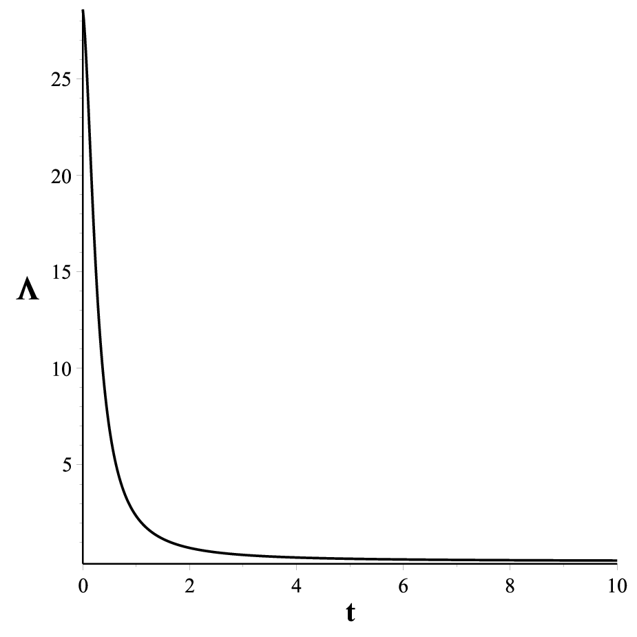
We see in Fig. (3) the variation of cosmological constant with respect to time, where is a decreasing function of time and it approaches a small positive value at late time.

VI The stability conditions
In this section, we are going to investigate the stability of the model. We can consider the stability by using the function . The stability condition occurs when the function becomes bigger than zero. The Fig. (3) shows the behavior of the speed of sound throughout the evolution of the universe. As we see, there is instability in early time and there is stability in late and future time.
VII Conclusion
In this paper, we have discussed the role of bulk and shear viscosity in Bianchi type-VI cosmological model by assuming that in the presence of cosmological constant. The field equations have been solved exactly for the corresponding model. Analytical solutions for the Hubble’s parameter, energy density, pressure, scale factor, volume scale and EOS parameter have been derived. Finally, we checked our calculation with several figures. For example in Fig. (1), the volume of the universe and Hubble parameter draw with respect to time and shown that during of evolution universe they are increasing and decreasing respectively. Also we saw in Fig. (2), decreases with respect to time and increases with respect to time. This lead us to have negative pressure and it is very large in early time. Also the EOS parameter crosses over phantom divided-line ()( also decreases with respect to time). The behavior of cosmological constant with respect to cosmic time is given by Fig. (3). In (3) we also observed that the term is initially infinite and it is decreasing function of time that approaches to zero at late time. Also, the stability of such system can be shown by Fig. (3) which is plot of the square of sound speed versus cosmic time.
References
- [1] Perlmutter, S., et al.: Astrophys. J.517, 5 (1999)
- [2] Riess, A.G., et al.: Astron. J.116, 1009 (1998)
- [3] Amirhashchi, H., Pradhan, A., Saha, B.: Astrophys. Space Sci.333, 295 (2011)
- [4] Amirhashchi, H., Pradhan, A., Saha, B.: Chin. Phys. Lett.3, 039801 (2011)
- [5] Pradhan, A., Amirhashchi, H., Saha, B.: Int. J. Theor. Phys.50, 2923 (2011)
- [6] Pradhan, A., Amirhashchi, H., Saha, B.: Astrophys. Space Sci.333, 343 (2011)
- [7] Saha, B.: Phys. Rev. D69, 124006 (2004)
- [8] Saha, B.:arXiv:1209.6029[gr-qc] (2012)
- [9] Socorro, J., Medina, E.R.: Phys. Rev. D61, 087702 (2000)
- [10] Weaver, M.: Class. Quantum Gravity17, 421 (2000)
- [11] Yadav, A.K., Saha, B.: Astrophys. Space Sci.337, 759 (2012)
- [12] Saha, B., Rikhvitsky, V.: Physica D219(2), 168176 (2006)
- [13] Desikan, K.: Gen. Relativ. Gravit.32, 14291438 (2000)
- [14] Saha, B.: Rom. Rep. Phys.57(1), 724 (2005)
- [15] Barrow, J.D.: Nucl. Phys. B310, 743 (1988)
- [16] Li, B., Barrow, J.D.: Phys. Rev. D79, 103521 (2009)
- [17] Xin-He, M., et al.: Commun. Theor. Phys.47, 379 (2007)
- [18] Patel, L.K., Koppar, S.S.: J. Aust. Math. Soc. Ser. B, Appl. Math33, 7784 (1991)
- [19] Bali, R., Pradhan, A., Amirhashchi, H.: Int. J. Theor. Phys.47, 2594 2604 (2008)
- [20] Bali, R., Banerjee, R., Banerjee, S.K.: Astrophys. Space Sci.317, 21 26 (2008)
- [21] Saha, B.: Gravit. Cosmol.16, 160 (2010)
- [22] Saha, B., Visinescu, M.: J. Rom. Phys.55, 1064 (2010)
- [23] Saha, B., Amirhashchi, H., Pradhan, A.: Astrophys. Space Sci.342(1), 257267 (2012)
- [24] Thorne, K.S.: Astrophys. J.148, 51 (1967)
- [25] Poplawski, N.J.: Phys. Rev. D74, 084032 (2006)
- [26] Carroll, S.M.: Living Rev. Relativ.4, 1 (2001). arXiv:astro-ph/ 0004075
- [27] Verma, M.K., Ram, S.: Appl. Math.2, 348354 (2011)
- [28] Sahani, V., Starobinsky, A.: Int. J. Mod. Phys. D9, 373443 (2000)
- [29] Poplawski, N.J.:arXiv:gr-qc/0608031(2006)
- [30] Harko, T., Lobo, F.S., Nojiri, S.I., Odintsov, S.D.: Phys. Rev. D84, 024020 (2011)