A multi-level solver for Gaussian constrained CMB realizations

The details of changing between pixel domain and spherical harmonic domain are usually glossed over in the literature. Since we will be solving a large linear system that couples signals on all scales — from individual pixels to the full sky — it is of the utmost importance to be precise about how these conversions are performed. If implemented incorrectly, even small pixel-scale errors can lead to overall divergence of the entire method.

There is no perfect grid on the sphere, and in choosing a particular one, a number of trade-offs must be considered. In our current implementation we adopt both the HEALPix¹¹ 1 http://healpix.sourceforge.net pixelization [14] and the Gauss-Legendre spherical grid [27, and references therein]. The HEALPix software package contains routines that are useful for our pixel domain computations, while the latter is required for accurate evaluation of Equation (2) below.

Given such a grid on the sphere (by which we mean a set of positions $\hat{n}_{i}$ on the sky), we can use spherical harmonic synthesis to transform a field expressed in spherical harmonic basis, with coefficients $s_{\ell m}$, to a field sampled on the sphere,

We will write this operation in matrix form as $\widehat{\mathbf{s}}=\mathbf{Y}\mathbf{s}$, where $\mathbf{Y}$ encodes the value of the spherical harmonics evaluated at each $\hat{n}_{i}$ of the chosen grid. Note that $\mathbf{Y}$ is not a square matrix, as spherical grids need to over-sample the signal to faithfully represent it up to some bandlimit ${\ell_{\text{max}}}$. In typical applications there are between $30\%$ and $100\%$ more pixels along the rows of $\mathbf{Y}$ than there are spherical harmonic coefficients along the columns. For the purposes of our method, it will turn out that we need to under-pixelize the signal instead, so there will be more columns than rows in $\mathbf{Y}$.

The opposite action of converting from pixel basis to harmonic basis is spherical harmonic analysis, which generally takes the quadrature form

where $w_{i}$ combines quadrature weights and pixel area. Similar to the synthesis case, this operation can be written in matrix form as $\mathbf{s}=\mathbf{Y}^{T}\mathbf{W}~\widehat{\mathbf{s}}$, where $W_{ij}=w_{i}\delta_{ij}$. A crucial feature of our method is the ability to (for the most part) avoid spherical harmonic analysis, however. Instead, we will rely on adjoint spherical harmonic synthesis, $\mathbf{Y}^{T}$, which simply appears algebraically as the transpose of $\mathbf{Y}$.

Note that, unlike in the case of the more famous discrete Fourier transform, $\mathbf{Y}$ is not a square orthogonal matrix, and synthesis and analysis differ by more than transposition and a scale factor. One may in some situations have that $\mathbf{Y}^{T}\mathbf{W}\mathbf{Y}=\mathbf{I}$, but this depends on both ${\ell_{\text{max}}}$, $N_{\text{pix}}$ and the spherical grid.

The action of applying $\mathbf{Y}$, $\mathbf{Y}^{T}$, $\mathbf{Y}^{T}\mathbf{W}$ or $\mathbf{W}\mathbf{Y}$ to a vector is in general referred to as a spherical harmonic transform (SHT). Carefully-optimized libraries are available that perform SHTs in $O({\ell_{\text{max}}}N_{\text{pix}})$ time; we use the libsharp library [28].

We now define our data model, and assume from the beginning that the CMB is Gaussian and isotropic [25, e.g.]. Following the notation of Eriksen et al. [9], it is convenient to define the CMB signal to be a vector $\mathbf{s}$ of spherical harmonic coefficients, in which case the associated covariance matrix $\mathbf{S}$ is given by

where $C_{\ell}$ is the CMB power spectrum.

Using the notation of the previous section, the model for the observed sky map pixel vector, $\mathbf{d}$, is

where $\mathbf{B}$ denotes beam-smoothing and the pixel window function, $\mathbf{n}$ is Gaussian instrumental noise, and the subscript of $\mathbf{Y}_{\text{obs}}$ indicates projection to the pixelization of the map $\mathbf{d}$.

We assume a symmetric instrumental beam, so that the beam matrix $\mathbf{B}$ is a diagonal matrix given by $B_{\ell m,\ell^{\prime}m^{\prime}}=b_{\ell}p_{\ell}\delta_{\ell\ell^{\prime}}\delta_{mm^{\prime}}$, where $b_{\ell}$ is the instrumental beam and $p_{\ell}$ the pixel window function of the observed grid. We also assume white instrumental noise, such that the noise covariance matrix, $\mathbf{N}$, is diagonal. We discuss the likely impact of asymmetric beams and correlated noise in Section V.

Discretization of the model is done simply by picking some ${\ell_{\text{max}}}$ for the $\mathbf{s}$ vector. The noise vector $\mathbf{n}$ is related to the map-making process, averaging the noise of time-ordered data (TOD) that fall within the same pixel, and so is inherently discrete rather than being a discretization of any underlying field. As already mentioned above, no spherical harmonic analysis of $\mathbf{d}$ (and therefore $\mathbf{n}$) is required when solving the CR system; rather, one solves for the projected $\mathbf{s}$, and so the noise treatment is always perfectly consistent with the assumed model.

Given the data model above, we are interested in exploring the Bayesian posterior distribution $p(\mathbf{s}|\mathbf{d},C_{\ell})$, the CMB signal given the data and CMB power spectrum. Let us first define

where in what follows we will refer to the first term as the prior term, and the second as the inverse-noise term. It can be shown that if we now solve the CR system

the solution $\mathbf{x}$ will be the maximum likelihood estimate of $\mathbf{s}$. Alternatively, if particular random fluctuation terms are added to the right-hand side of Eq. (5), the solution $\mathbf{x}$ will instead be samples from the posterior [20, 35]. Since $b_{\ell}\to 0$ as $\ell$ increases, the diagonal prior term will at some point dominate the dense inverse-noise term, so that truncation at sufficiently high ${\ell_{\text{max}}}$ does not affect the solution of the system.

As stressed in Section II.1, $\mathbf{Y}_{\text{obs}}^{T}$ denotes spherical harmonic adjoint synthesis, and not spherical harmonic analysis. Pixels that are masked out, typically due to strong foreground contamination, are simply missing from the data vector $\mathbf{d}$, and so the corresponding rows are not present in $\mathbf{Y}_{\text{obs}}$. This means $\mathbf{Y}_{\text{obs}}$ is not an orthogonal matrix, but that is not a concern since we never perform spherical harmonic analysis of pixels on the observation grid. The solution $\mathbf{x}$ is still well-defined everywhere on the sky due to the prior term $\mathbf{S}^{-1}$. This is typically implemented by introducing zeroes in $\mathbf{N}^{-1}$ rather than removing rows of $\mathbf{Y}_{\text{obs}}$, which has the statistical interpretation of giving those pixels infinite variance. The two interpretations are algebraically equivalent.

The CR system in Equation (4) is symmetric and positive definite, which suggests the use of the Conjugate Gradient (CG) algorithm. For the behavior of CG and other Krylov methods, we are primarily interested in the eigenspectrum after preconditioning [31, and references therein], i.e. the eigenspectrum of $\mathbf{M}\mathbf{A}$, where $\mathbf{M}\approx\mathbf{A}^{-1}$. To illustrate the fundamental problem with the CG algorithm for the application considered here, we show in Figure 1 the eigenspectrum of a low-resolution setup, using a diagonal preconditioner. This case corresponds to a simulation of the 143 GHz Planck frequency map [23], downgraded to an angular resolution of $5.4^{\circ}$, bandwidth-limited at $\ell_{\textrm{max}}=95$, and with a mask applied that removes 40% of the sky. The overall shape of the spectrum appears to be mostly independent of the resolution, with a significant fraction of degrees of freedom found in the tails. This behavior is representative of that found in real-world cases.

The problematic feature is the exponential drop in the eigenvalues seen to the left of the figure. Theoretical results indicate that the CG search needs at least one iteration per eigenvalue located in exponentially increasing parts of the eigenspectrum [1, 2]. This leads to extreme degradation of CG performance, which is indeed what has been observed with Commander on high-resolution, high-sensitivity data.

The exponential spectral feature is due to large-scale modes under the mask. For all but the smallest angular scales, the $\mathbf{N}^{-1}$ term dominates by many orders of magnitude, so that the $\mathbf{S}^{-1}$ term is hardly seen at all. However, vectors that only build-up signal under the mask after beam-smoothing will only see the $\mathbf{S}^{-1}$ term of the matrix, as the $\mathbf{N}^{-1}$ term vanishes in that case. The eigenvectors corresponding to the smallest eigenvalues are therefore characterized by having large scales localized within the mask. Moreover, the solution under the mask is constrained by the values at the mask edge, meaning the $\mathbf{N}^{-1}$ term takes effect, and this constraint is harder closer to the edges. The result is an exponentially-falling eigenspectrum, rather than separated clusters of eigenvalues that CG could more easily deal with.

Phrased differently, for data having a high signal-to-noise ratio, the pixels near the edge of the mask carry a large predictive power on the signal inside the mask — a signal that must be reconstructed by the CG algorithm by navigating through a nearly degenerate system. In total, the CG convergence rate is determined by a combination of the overall signal-to-noise ratio and the size and shape of the mask. We have been unable to achieve proper convergence with this method for the signal-to-noise ratio of a Planck-like experiment, for example, independent of preconditioners or number of iterations; downgrading and adding regularization noise is required to produce robust results.

The matrix $\mathbf{A}$ of Equation (4) is defined in spherical harmonic domain, and describes the coupling strength between pairs of $(\ell,m)$ and $(\ell^{\prime},m^{\prime})$. Except in unrealistic scenarios with very simple instrumental noise and mask, we have found no pattern in the magnitudes of the matrix coefficients $A_{\ell m,\ell^{\prime}m^{\prime}}$ that is consistent enough to be exploited in a solver.

By moving to pixel domain, however, we can create such an exploitable pattern in the magnitudes of the matrix coefficients. In Section III.3 we will construct a corresponding pixel-domain matrix $\widehat{\mathbf{A}}$ that is localized, in the sense that $\widehat{A}_{ij}$ has small magnitude (less than $1\%$ of $\widehat{A}_{ii}$) unless pixels $i$ and $j$ are very close together on the sphere.

It is no surprise that the $\mathbf{N}^{-1}$ term of Equation (4) enjoys this property, since we have assumed that instrumental noise is uncorrelated between pixels. When it comes to the $\mathbf{S}^{-1}$ term, we note that $1/C_{\ell}$ is roughly proportional to $\ell(\ell+1)$, at least for $\ell\lesssim 1000$. These are the eigenvalues of the Laplacian on the sphere, with $\mathbf{Y}$ being the corresponding eigenbasis. Therefore we can hope that a projection of $\mathbf{S}^{-1}$ to pixel domain should be close to a Laplacian. The Laplacian is often approximated with a matrix where $\widehat{A}_{ij}=0$ unless pixel $i$ and $j$ are neighbors or $i=j$. While our case will be less perfect, it still suggests that multi-level methods can be very efficient, since those are highly successful for PDEs involving the Laplacian.

In Section III.5, we exploit the localization properties in pixel domain to develop an approximate inverse $\widehat{\mathbf{M}}\approx\widehat{\mathbf{A}}^{-1}$. Figure 2 demonstrates the use of this approximate solver as part of a simple stationary method

where we initialize $\mathbf{x}\leftarrow\mathbf{0}$ and then iteratively update the solution. Note that if we replace $\widehat{\mathbf{M}}$ with $\text{diag}(\mathbf{A})^{-1}$, Eq. (6) represents what are known as Jacobi iterations.

The problem that is evident from Figure 2 is that $\widehat{\mathbf{M}}$ will only make improvements to one part of the frequency spectrum — namely, the highest frequencies that can be represented on the grid used. This is the typical case when multi-level methods are applied; iterations of the form of Equation (6) are usually only efficient at resolving the relations between pixels/elements that are strongly coupled, which, when $\widehat{\mathbf{A}}$ is localized, translates to resolving the solution at highest frequencies. Little or no improvement is made between pixels that are weakly or indirectly coupled in $\widehat{\mathbf{A}}$, so that no improvement is made to the coarser scales. Put another way, the error, $\mathbf{e}\equiv\mathbf{x}-\mathbf{x}_{\text{true}}$, has its high-frequency components reduced, while the low frequencies are left relatively unaffected. The approximate inverse $\widehat{\mathbf{M}}$ is therefore dubbed a smoother in multi-level terminology. We will use the term error smoother to distinguish it from the act of applying a low-pass filter (which is instead called restriction in this context).

The key is now to project the matrix $\mathbf{A}$ to pixel grids at different resolutions, producing a set of matrices $\widehat{\mathbf{A}}_{h}$, where $h$ is a level indicator. For each $\widehat{\mathbf{A}}_{h}$ we construct a corresponding error smoother $\widehat{\mathbf{M}}_{h}\approx\widehat{\mathbf{A}}_{h}^{-1}$ that resolves the errors in one region of the frequency spectrum only. Using these levels together, we arrive at a method that converges very well over the entire frequency spectrum.

In this section we give a brief overview of multi-level theory, together with the specification of our algorithm. For a more detailed introduction to multi-grid methods, consult one of the number of standard texts [17, e.g.]. Ingredients of multi-level algorithms are:

1. 1.

   A set of bases to project the linear system into in order to work on different parts of the solution. Usually these form a hierarchy of levels from finest to coarsest, so that each level solves for different frequencies of the solution. It is customary to label levels relatively, using $h$ for the current level and $H$ for the coarser level.

2. 2.

   A way to transfer vectors between the different levels. The restriction operator, $\mathbf{I}_{h}^{H}$, takes a vector from a finer level to a coarser level, while the interpolation operator $\mathbf{I}_{H}^{h}$ works in the opposite direction. For symmetric systems, one often takes $\mathbf{I}_{H}^{h}=(\mathbf{I}_{h}^{H})^{T}$.

3. 3.

   One linear operator (left-hand-side matrix) for each level. For the case where interpolation is chosen to be transposed restriction, these are often defined recursively as

   $$\mathbf{A}_{H}=\mathbf{I}_{H}^{h}\mathbf{A}_{h}(\mathbf{I}_{H}^{h})^{T}$$

   (7)

   for the projection of a fine matrix $\mathbf{A}_{h}$ to a coarser matrix $\mathbf{A}_{H}$.

4. 4.

   An error smoother $\mathbf{M}_{h}$ for each $\mathbf{A}_{h}$ that removes the higher frequencies of the error on level $h$, as discussed in the previous section.

Multi-level algorithms are often implemented on a grid or a tessellation in real space, with a sparse linear operator, and using averages of neighboring points as the restriction operator $\mathbf{I}_{h}^{H}$. In our case, $\widehat{\mathbf{A}}_{h}$ on each level is not sparse, and, at least without approximations, multiplying $\widehat{\mathbf{A}}_{H}=\mathbf{I}_{H}^{h}\widehat{\mathbf{A}}_{h}\mathbf{I}_{h}^{H}$ with a vector would be computationally very expensive on the coarser levels as it would require interpolating back to the highest-resolution grid.

To avoid this cost, we instead define our levels in spherical harmonic domain. Let $\tilde{f}_{\ell}^{h}$ be a spherical harmonic low-pass filter that emphasizes one part of the frequency spectrum, and define $\mathbf{F}_{h}$ to be a diagonal matrix with elements $\tilde{f}_{\ell}^{h}$. We then define

where the prior term $\mathbf{D}_{h}$ is diagonal with entries given by $(\tilde{f}^{h}_{\ell})^{2}/C_{\ell}$ and the modified beam matrix $\mathbf{B}_{h}$ is diagonal with elements given by $\tilde{f}^{h}_{\ell}b_{\ell}p_{\ell}$. In this case, the system is bandlimited by some ${\ell^{h}_{\text{max}}}\leq{\ell_{\text{max}}}$, above which $\tilde{f}^{h}_{\ell}=0$. Figures 3 and 4 show the filters used in our setup; we discuss the choice of filters further in Section III.3.

With this choice, we can clearly satisfy the multi-level hierarchy of Equation (7) by choosing the restriction operator $\mathbf{I}_{h}^{H}$ as an $(\ell_{\text{max}}^{H}+1)^{2}$-by-$(\ell_{\text{max}}^{h}+1)^{2}$ block matrix, where the block for $\ell\leq\ell_{\text{max}}^{H}$ is diagonal with entries

and the block for $\ell_{\text{max}}^{H}<\ell\leq\ell_{\text{max}}^{h}$ is zero.

As already mentioned in Section III.1, the error smoother that we have available, $\widehat{\mathbf{M}}_{h}$, is defined in pixel domain. For every spherical harmonic (SH) level we therefore tag on a corresponding sibling pixel level with matching HEALPix resolution $N^{h}_{\text{side}}$. The result is the following level structure:

The arrows indicate that transfers between different scales happen only through the spherical harmonic levels. As emphasized in Section II.1, no spherical harmonic analysis operations are performed in each conversion (only synthesis and adjoint synthesis operations), and the implied under-pixelization in the above scheme is therefore numerically unproblematic.

The full details of how to properly move between the levels to obtain a solution is given in pseudo-code in Figure 5. We highlight some aspects in what follows.

Assume that we are currently on some spherical harmonic level $h$ (where the original equation is simply the top level), with corresponding system

We start with some search vector $\mathbf{x}_{h}$ (initialized to zero), and want to improve it to get closer to the true value $\mathbf{x}_{\text{true},h}$. In order to make use of $\widehat{\mathbf{M}}$, we must now move to the corresponding pixel level. Our chosen restriction operator, denoted $\mathbf{Y}_{h}$, is spherical harmonic synthesis to a HEALPix grid²² 2 The pixel level is actually coarser than the spherical harmonic level, because ${\ell^{h}_{\text{max}}}$ must be chosen so high that the grid cannot resolve all the scales of the projected field. See Section III.4. of resolution $N^{h}_{\text{side}}$. The key to efficient multi-level solvers is to transfer the residual vector $\mathbf{r}_{h}$, and not the search vector $\mathbf{x}_{h}$;

where $\widehat{\mathbf{r}}_{h}$ is the pixel domain projection of $\mathbf{r}_{h}$. Then, we approximately solve the projected system for a correction vector $\widehat{\mathbf{c}}_{h}$,

where the computation of $\widehat{\mathbf{M}}\,\widehat{\mathbf{r}}_{h}$ is further described in Section III.5. The approximation is better for small scales than for large scales. Finally, we let the interpolation operator be the transpose of restriction, $\mathbf{Y}^{T}$, so that the correction is brought over to the spherical harmonic search vector by adjoint spherical harmonic synthesis,

Together, these steps act as the error smoothing of a spherical harmonic level, labeled pre- and post-smoothing in Figure 5. Here we have motivated the procedure as arising from moving between levels, but the idea of solving for a correction in a projected system arises in many settings [33], and other variations on this theme may prove fruitful in the future.

The vertical movement between coarser and finer levels follows the same pattern, but uses the restriction operator $\mathbf{I}_{h}^{H}$ defined in Equation (9) instead of pixel projection $\mathbf{Y}$. First, a fine residual is computed and restricted (i.e. low-pass filtered) to the coarser level,

Then, a coarse correction $\mathbf{c}_{H}$ is sought that approximates the solution of the coarse system

Except for at the bottom level, this happens by initializing a search vector $\mathbf{c}_{H}$ to zero and recursively applying the algorithm. Finally, the correction is interpolated and applied to our current search vector,

Using this idea of transferring residuals and corrections between levels with different bases, one can form a variety of multi-level cycles, moving between the levels in different patterns. Our choice in the end is a W-cycle on the coarser levels and a V-cycle on the finer levels, as described in Section IV.1 and the pseudo-code.

In addition to the pixel levels described above, the top and bottom levels are special. The smallest scales ($\ell\gtrsim 2200$ in our experimental setup) are strongly noise-dominated, making the spherical harmonic domain matrix $\mathbf{A}$ nearly diagonal. As a result, we do not project to a pixel grid, but simply use $\text{diag}(\mathbf{A})^{-1}$ as the error smoother. Note, however, that this process would destroy the solution on scales that are not entirely noise-dominated, and so we first apply a high-pass filter to the correction vector before applying it to the solution search vector. For the largest scales ($\ell\leq 40$), we do not project to pixel domain either, but simply solve $\mathbf{A}\mathbf{x}=\mathbf{b}$ restricted to $\ell\leq 40$ by explicitly computing the matrix entries and using a simple Cholesky solver.

For the top solver level, we need to compute the diagonal of $\mathbf{Y}_{\text{obs}}^{T}\mathbf{N}^{-1}\mathbf{Y}_{\text{obs}}$ in spherical harmonic domain, and for the bottom solver level we similarly need all entries of $\mathbf{Y}_{\text{obs}}^{T}\mathbf{N}^{-1}\mathbf{Y}_{\text{obs}}$ for $\ell$ up to some $\ell_{\text{dense}}$. While such entries can be computed using Wigner 3j-symbols [19, 9], the following procedure has some significant advantages. Firstly, while the computational scaling is the same, it is much faster in practice, in particular due to the optimized code for associated Legendre polynomials $P_{\ell m}$ available in libpsht [27]. Secondly, it is accurate to almost machine precision for any grid, whereas the method relying on Wigner 3j-symbols relies on approximation by evaluation of an integral, and is therefore inaccurate for low-resolution HEALPix grids.

Let $\xi_{kj}$ be the $j$-th of $J_{k}$ pixels on ring $k$ in the masked inverse-noise map. One can then evaluate

where the normalized associated Legendre function is

The inner sum can be precomputed for each ring $k$ and every $(m_{1}-m_{2})$ by discrete Fourier transforms, allowing the evaluation of matrix elements in $O(N_{\text{ring}})=O({\ell_{\text{max}}})$ time. In the case that we want a dense low-$\ell$ block, the procedure to downgrade the inverse-noise operator from Section III.4 should be applied first, to reduce the computational cost from $O(\ell_{\text{dense}}^{2}{\ell_{\text{max}}})$ to $O(\ell_{\text{dense}}^{3})$.

So far we have not specified the exact form of the low-pass filters $\tilde{f}_{\ell}^{h}$ required for every level. It turns out that careful selection of these filters is essential to ensure that the pixel projection of $\mathbf{A}_{h}$ is localized, and hence that the construction of an efficient error smoother is possible.

As indicated in Eq. (13), the spherical harmonic system $\mathbf{A}_{h}$ on each level $h$ is projected to pixel domain with

where the prior and pixelized beam terms are this time given by (respectively)

Note that the pixelization along the rows of $\widehat{\mathbf{B}}_{h}$ is the observational grid, while the pixelization down the columns is that of the current level.

The matrices $\widehat{\mathbf{D}}_{h}$ and $\widehat{\mathbf{B}}_{h}$ are both rotationally invariant. By the addition theorem of spherical harmonics, the coupling strength between two points on the sphere separated by angular distance $\theta$ is given by

where we insert $g_{\ell}=(\tilde{f}^{h}_{\ell})^{2}/C_{\ell}$ for $\widehat{\mathbf{D}}_{h}$ and $g_{\ell}=\tilde{f}^{h}_{\ell}b_{\ell}p_{\ell}$ for $\widehat{\mathbf{B}}_{h}$. The pixel-domain localization of such matrices depends entirely on $g_{\ell}$. In our experience, the $g_{\ell}$ that lead to localized matrices in pixel domain tend to be flat or polynomially increasing before an exponential drop. Since $b_{\ell}$ already describes a localized beam, and $1/C_{\ell}$ increases non-exponentially, crafting a localized system $\widehat{\mathbf{A}}_{h}$ at each level is indeed possible.

Selecting the filters $f^{H}_{h,\ell}$, whose products form $\tilde{f}^{h}_{\ell}$ and $\mathbf{F}_{h}$ for each level, is a non-trivial matter. The main characteristic the filters must have is that each $\tilde{f}^{h}_{\ell}$ falls off quickly enough in real space to avoid strong couplings between the edge of the mask and the interior. Figure 6 shows what happens if this is not controlled correctly — the long-range couplings make the construction of an error smoother $\widehat{\mathbf{M}}$ impossible. In contrast, Figure 7 shows the behavior of the operators in the well-tuned case.

A filter that we found to work very well is given by squaring the exponent of a Gaussian,

The scale parameter $\lambda$ is simply chosen from the scale behavior that we want. In our test runs, we chose the constraints $q_{2570}=0.1$ at the $N^{h}_{\text{side}}\!\!=\!\!1024$ level and $q_{1536}=0.1$ at the $N^{h}_{\text{side}}=512$ level.

This filter has the following advantages over a simple Gaussian:

• •

  It decays much more quickly in $\ell$, while in real space it decays almost as quickly in the tails as the Gaussian. This allows us to avoid increasing the bandlimit of the original system beyond ${\ell_{\text{max}}}=3000$.

• •

  The rapid decay with $\ell$ is also beneficial to counter the behavior of $1/C_{\ell}$. In the range $2000<\ell<3000$, $1/C_{\ell}$ follows a rather steep trajectory (between $\sim\ell^{7}$ and $\ell^{8}$) which, when only countered by a Gaussian, causes some ringing and less locality.

• •

  Using Gaussian filters shapes the $\mathbf{N}^{-1}$ term so that couplings around a given pixel are similar to a Gaussian with FWHM of 4 pixels. That is, the couplings between neighboring pixels are rather strong. The filter defined above produces much weaker couplings between neighbors. This is not currently an advantage, because we let every pixel “see” a radius of $k=8$ pixels around itself anyway in the error smoother. However, it could become an advantage in the future if $k$ is chosen adaptively for each pixel.

Despite these features, the simple Gaussian filter behaved better at the coarser levels with very high signal-to-noise, as can be seen by comparing the second panel of Figure 7 with the first panel of Figure 8. In our tests we chose a Gaussian filter $f_{h,\ell}^{H}$ for levels $N^{h}_{\text{side}}\leq 256$, tuned so that the cumulative filter $\tilde{f}_{\ell}^{h}$ on each level roughly corresponds to a Gaussian with FWHM of 2 pixels.

Figure 9 shows the effect of choosing the bandlimit ${\ell^{h}_{\text{max}}}$ too low. On the coarser levels, ringing from the inverse-noise term causes strong non-local couplings unless the bandlimit is set as high as $6N^{h}_{\text{side}}$. This limit depends on the signal-to-noise ratio, and ${\ell_{\text{max}}}=4N^{h}_{\text{side}}$ is sufficient on the $N_{\text{side}}=512$ level.

The HEALPix grid can only represent a field accurately up to ${\ell^{h}_{\text{max}}}\sim 2N^{h}_{\text{side}}$, and will in fact see different scales on different parts of the sphere, due to the necessary irregularities in the pixelization. This is the primary reason for the non-traditional level traversal structure chosen in Section III.2. The pixel projection operator $\mathbf{Y}_{h}$ removes some parts of the projected field that the grid cannot represent, but this is after all how a multi-level restriction normally works, and so poses no problems.

The filter $\tilde{f}_{\ell}^{h}$ allows us to set ${\ell^{h}_{\text{max}}}$ much lower than the full ${\ell_{\text{max}}}$. The two SHTs involved in $\mathbf{Y}_{\text{obs}}^{T}\mathbf{N}^{-1}\mathbf{Y}_{\text{obs}}$ still involve an $N_{\text{side}}=2048$ grid, however, so the coarsest levels are still almost as computationally expensive as the finest levels.

To work around this, the key is to note that the operator $\mathbf{Y}_{\text{obs}}^{T}\mathbf{N}^{-1}\mathbf{Y}_{\text{obs}}$ does not “see” scales in the inverse-noise map beyond $2{\ell^{h}_{\text{max}}}$. This follows from an expansion into Wigner 3j-symbols [19, 9]. Simply degrading the inverse-noise map to a coarser resolution HEALPix grid was found to be far too inaccurate, so more care is needed. First, we rewrite the operator as

where $\mathbf{W}_{\text{obs}}$ denotes the quadrature weights of the HEALPix $N_{\text{side}}=2048$ grid, so that $\mathbf{Y}_{\text{obs}}^{T}\mathbf{W}_{\text{obs}}$ corresponds to spherical harmonic analysis, as described in Section II.1. Then, we write $\xi_{i}$ for the pixels on the diagonal of $\mathbf{W}^{-1}\mathbf{N}^{-1}$, and $\xi_{\ell m}$ for the same map expanded into spherical harmonics. Since the operator of Equation (25) does not see coefficients beyond $2{\ell^{h}_{\text{max}}}$, we can truncate $\xi_{\ell m}$ and project it onto a Gauss-Legendre grid of the same order, which (unlike HEALPix grids) allows spherical harmonic analysis that is accurate to almost machine precision. Using this re-weighted and downgraded inverse-noise map as the diagonal of a new inverse-noise matrix $\tilde{\mathbf{N}}^{-1}_{h}$, we have that

where $\tilde{\mathbf{Y}}_{h}$ and $\tilde{\mathbf{Y}}^{T}_{h}\tilde{\mathbf{W}}_{h}$ indicate spherical harmonic synthesis and analysis on the Gauss-Legendre grid.

A simple diagonal error smoother does not converge in our setup, primarily because pixels on the edge of the mask can have a very strong influence on the solution in the interior of the mask, as seen in Figure 7. Also, when applying Gaussian filters, the couplings between neighboring pixels are rather strong, preventing the use of a diagonal error smoother even far from the mask.

The basic strategy for our error smoother is to make sure that every pixel “sees” neighboring pixels in some radius $k$ around it. In our case we let $k=8$ on all levels, although improvements on this may be possible, especially in cases with lower signal-to-noise than ours.

We start by dividing the sphere into tiles of size $k$-by-$k$. Then, we include the couplings between pixels in the same and neighboring tiles while ignoring any couplings between pixels further apart, so that couplings are included in a radius of at least $k$ pixels around every pixel. The result is a block sparse matrix, as shown in Fig. 10.

Next, we explicitly compute the parts of $\widehat{\mathbf{D}}_{h}$ (Eq. (21)) and $\widehat{\mathbf{B}}_{h}$ (Eq. (22)) that fall within the sparsity pattern by evaluating the sum over Legendre polynomials from Equation (23). After preparing the block sparse matrix approximations, we use matrix multiplication without fill-in to compute $\widehat{\mathbf{B}}^{T}\mathbf{N}^{-1}\widehat{\mathbf{B}}$ — that is, we neglect resulting blocks outside of the same sparsity pattern. The approximant for $\widehat{\mathbf{D}}_{h}$ can then be added directly. Finally, we perform a zero-fill-in Incomplete Cholesky factorization (ICC), i.e. we perform in-place Cholesky factorization of the block sparse approximant as usual, but ignore any element updates outside of the sparsity pattern during the factorization process.

Without modification, the factorization process usually fails, either due to the sparse approximant of the full dense matrix ending up non-positive-definite, or because of elements dropped during the ICC. When this happens, we do a binary search for the lowest ridge adjustment $\alpha$ that, when added to the diagonal, makes the factorization procedure succeed, and scale this $\alpha$ by a factor of $1.5$ for the final factorization. Typical ridge values $\alpha$ are in the range $10^{-2}$ to $10^{-4}$ times the maximum element of $\mathbf{A}_{h}$.

After factorization, applying the smoother is simply a matter of doing the usual triangular solve. This is an inherently sequential process, and the smoother therefore currently runs on a single CPU core. Since an error smoother only needs to work locally, we expect to be able to apply domain decomposition techniques, partitioning the sphere into large domains that overlap by $k$ or $2k$ pixels, and applying one error smoother on each domain. Proper parallelization of the error smoother is left for future work, however. Also note that the process described above is the very simplest incomplete factorization algorithm, and more sophisticated incomplete factorization algorithms are standard in the literature.

In Section IV.1, we quote numbers for the execution time and memory usage of the smoother. One possibility for reducing memory consumption in the future is to let $k$ be adaptive, as it can be made smaller away from the edges of the mask. All error smoother computations are done in single precision. In the current implementation, computing $\widehat{\mathbf{B}}$ is very expensive, as we sample it directly on the $N_{\text{side}}=2048$ grid. This is not a fundamental scaling problem, but rather an issue of implementation, as the degraded inverse-noise map on the Gauss-Legendre grid described in Section III.4 could also be used in this setting.

The basic assumptions for our experimental setup have already been laid out in Section II.2. We choose for our example the RMS map and symmetric beam approximation of the 143 GHz channel of Planck, as provided in the Planck 2013 data release [23].

We tried running both with the 40%-sky, 80%-sky and 97%-sky masks used in the Planck analysis, in all cases together with the 143 GHz point source mask. The mask has some impact on speed of convergence, but not enough to warrant attention, and we therefore only present the results from the 80%-sky mask, which was the slowest to converge.

For the power spectrum, $C_{\ell}$, we use the standard best-fit Planck+WP+high-$\ell$ 6-parameter $\Lambda$CDM spectrum [26], but set $C_{0}$ and $C_{1}$ to the value of $C_{2}$ as a wide prior for any residual monopole or dipole component. Statistically, the prior for the monopole and dipole is of little relevance, since the data so strongly constrain these components. Note that the present algorithm will not let us condition on a given monopole and dipole (i.e. set $C_{0}=C_{1}=0$), at least without modifications.

To produce the right-hand side, $\mathbf{b}$, corresponding to a random test realization, we draw a simulated $\mathbf{x}_{\text{true}}$ from the prior $p(\mathbf{s}|C_{\ell})$, and multiply it with $\mathbf{A}$ of Equation (4). This synthetic setup allows us to track the true error, $\mathbf{e}=\mathbf{x}_{\text{true}}-\mathbf{x}$. In a real setting the right hand side is of course generated from observed data, and in this case one can only track the residual, $\mathbf{r}=\mathbf{b}-\mathbf{A}\mathbf{x}$.

The error smoothers are least efficient on the largest scales. At the same time, these are much cheaper to process than the small-scale smoothers due to the $O(\ell^{3}_{\text{max}})$ scaling of the spherical harmonic transforms. We therefore choose a partial W-cycle, where the levels for $N^{h}_{\text{side}}\leq 1024$ participate in a W-cycle ($n_{\text{rec}}^{h}=2$ in Figure 5), but the very expensive error smoother of the $N^{h}_{\text{side}}=1024$ level, as well as SHTs at ${\ell_{\text{max}}}=3000$, are only run once on the way down and once on the way up (a V-cycle).

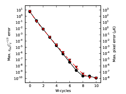
In Figure 11 we plot the resulting convergence, in terms of absolute error as a function of W-cycle iteration count. Here we see that the error falls exponentially with cycle count, at the rate of roughly one order of magnitude per iteration. The largest error anywhere on the sky is smaller than $1\mu\textrm{K}$ after only 3 W-cycles, and approaches the numerical precision limit after 8 cycles.

As mentioned above, since we know what the true solution is for the simulated data, we are also able to trace the absolute error, $\mathbf{e}=\mathbf{x}_{\text{true}}-\mathbf{x}$, although only the residual, $\mathbf{r}=\mathbf{b}-\mathbf{A}\mathbf{x}$, is available in real-world applications. Figure 12 shows that these have qualitatively very similar behavior as a function of W-cycle count, which implies that the residual can be used as a robust proxy for the actual error for the multi-level algorithm. The same is not true for the CG method, for which the error can flatten earlier than the residual due to the presence of the nearly singular modes in $\mathbf{A}$.

Finally, in Figure 13 we show the relative error as a function of multipole moment and W-cycle count. This plot highlights the problematic angular scales, and is therefore particularly useful during the debugging and tuning phase of the analysis; for example, the use of a V-cycle rather than a W-cycle would make the large scales noticeably lag behind in convergence on this plot. Another example is that, if the filters $\tilde{f}_{h}$ are poorly-tuned (potentially causing the method to diverge), the responsible level can often be picked out on this plot.

The total run-time for this setup was 114 seconds wall time per W-cycle on 16 CPU cores (AMD 6282 running at 2.6 GHz). Table 1 breaks this cost down further to the individual levels and actions. The bulk of the memory use is by the error smoothers, which consume about 20 GiB of memory (see Table 2). The total process footprint was around 30 GiB, although unnecessary temporary arrays abound in the current implementation.

Table 2 presents the cost of the necessary precomputations. For every new combination of instrumental beam, noise map and mask, or for a new choice of multi-level filters $f_{h,\ell}^{H}$, one needs to precompute an approximation to $\widehat{\mathbf{B}}_{h}^{T}\mathbf{N}^{-1}\widehat{\mathbf{B}}_{h}$ for every solver level. These precomputations required a total of 44 CPU hours in our tests, but are trivially parallel. We also expect that one will usually load the results from disk. The approximation for $\widehat{\mathbf{D}}_{h}$ must be recomputed every time $C_{\ell}$ changes, which in the case of Gibbs sampling means every time one wants to run the solver. Fortunately, this computation is much cheaper and only requires around 100 CPU minutes of trivially parallel work, plus 2 minutes of non-parallel work. We argue in Section V that it should be possible to greatly decrease precomputation time in future.

The main weakness in the current implementation is the lack of parallelization in the error smoothers. Not only does the code need to be run on a single node, but the 40 seconds spent on error smoothing runs on a single CPU core, with the 15 other cores idling. Parallelization of the smoother would bring the wall time much closer to 80 seconds, as well as allowing the distribution of the 20 GiB of smoother data among several cluster nodes.

The CR solver is part of Commander 2, which is made available as open source software under the BSD license (core code) and the GPL license (full software when including dependencies). For more information, see http://commander.bitbucket.org/.

Commander 2 is implemented in a mixture of Python (using NumPy and SciPy), Cython [3], Fortran 90, and C. For SHTs we use libsharp [28]. For our benchmarks we have used OpenBLAS [16, 36] for linear algebra.

The main computation time is spent in libsharp or OpenBLAS, and as such is already highly optimized. The computation of Equation (23) benefited greatly from being structured as described in the appendix of [29]. In addition to what is mentioned there, we made use of the AVX and FMA4 instruction sets. Also, note that all the computations for the error smoother could be performed in single precision.

References

- [1] Axelsson, O., & Lindskog, G. 1986, Numerische Matematik, 48, pp. 479
- [2] Axelsson, O., & Lindskog, G. 1986, Numerische Matematik, 48, pp. 499
- [3] Behnel, S., Bradshaw, R., Citro, C., Dalcin, L., Seljebotn, D. S., & Smith, K. 2011 Computing in Science & Engineering, 13, 2
- [4] Bennett, C. L., Larson, D., Weiland, J. L., et al. 2013, ApJS, 208, 20
- [5] Brandt, A. 2011, in Multiscale and Multiresolution Methods, ed. T. J. Barth et al. (Springer Verlag, Berlin), 1
- [6] Doré, O., Teyssier, R., Bouchet, F. R., Vibert, D., & Prunet, S. 2001, A&A, 374, 358
- [7] Elsner, F., & Wandelt, B. D. 2012, arXiv:1211.0585
- [8] Elsner, F., & Wandelt, B. D. 2013, A&A, 549, A111
- [9] Eriksen, H. K., O’Dwyer, I. J., Jewell, J. B., et al. 2004, ApJS, 155, 227
- [10] Eriksen, H. K., Huey, G., Saha, R., et al. 2007a, ApJ, 656, 641
- [11] Eriksen, H. K., Huey, G., Banday, A. J., et al. 2007b, ApJ, 665, L1
- [12] Eriksen, H. K., Jewell, J. B., Dickinson, C., et al. 2008a, ApJ, 676, 10
- [13] Eriksen, H. K., Dickinson, C., Jewell, J. B., et al. 2008b, ApJ, 672, L87
- [14] Górski, K. M., Hivon, E., Banday, A. J., et al. 2005, ApJ, 622, 759
- [15] Grigori, L., Stompor, R., Szydlarski, M. 2012, in Proc. of the Int. Conf. on High Performance Computing, Networking, Storage and Analysis (Salt Lake City, Utah), 91
- [16] Goto, K., & van de Geijn, R. 2008 ACM Trans. Math. Softw., 34, 3
- [17] Hackbush, W. 1985, Multi-grid methods and applications (Springer Verlag, Berlin)
- [18] Havé, P., Masson, R., Nataf, F., Szydlarski, M., Xiang, H., and Zhao, T. (2013) SIAM Journal on Scientific Computing, 35, 3
- [19] Hivon, E., Górski, K. M., Netterfield, C. B., Crill, B. P., Prunet, S., & Hansen, F. 2002, ApJ, 567, 2
- [20] Jewell, J., Levin, S., & Anderson, C. H. 2004, ApJ, 609, 1
- [21] Mitra, S., Rocha, G., Górski, K. M., et al. 2011, ApJS, 193, 5
- [22] O’Dwyer, I. J., Eriksen, H. K., Wandelt, B. D., et al. 2004, ApJ, 617, L99
- [23] Planck Collaboration, 2013a, A&A, submitted, [1303.5062]
- [24] Planck Collaboration, 2013b, A&A, submitted, [1303.5075]
- [25] Planck Collaboration, 2013c, A&A, submitted, [1303.5083]
- [26] Planck Collaboration, 2013d, A&A, submitted, [1303.5076]
- [27] Reinecke, M. 2011, A&A, 526, A108
- [28] Reinecke, M., & Seljebotn, D. S. 2013, A&A, 554, A112
- [29] Seljebotn, D. S. 2012, ApJS, 199, 5
- [30] Scodeller, S., Rudjord, Ø., Hansen, F. K., et al. 2011, ApJ, 733, 121
- [31] Shewchuk, J. R. 1994, http://www.cs.cmu.edu/quake-papers/painless-conjugate-gradient.ps
- [32] Smith, K. M., Zahn, O., & Doré, O. 2007, Phys. Rev. D, 76, 043510
- [33] Tang, J. M., Nabben, R., Vuik, C., Erlangga, Y. A. 2009, Journal of Scientific Computing, 39, 3
- [34] Wandelt, B. D., & Górski, K. M. 2001, Phys. Rev. D, 63, 123002
- [35] Wandelt, B. D., Larson, D. L., & Lakshminarayanan, A. 2004, Phys. Rev. D, 70, 083511
- [36] Xianyi, Z., Qian, W., Yunquan, Z., Model-driven Level 3 BLAS Performance Optimization on Loongson 3A Processor, 2012 IEEE 18th International Conference on Parallel and Distributed Systems (ICPADS)