跳到论文正文
W Papers独立论文阅读器 arXiv:1308.5207 论文正文 计算阅读时间 · 0%
引用这篇论文根据当前论文元数据生成,正式投稿前建议核对。


License: arXiv.org perpetual non-exclusive license
arXiv:1308.5207v4 [cs.DS] 06 Oct 2015

Approximating the Little Grothendieck Problem over the Orthogonal and Unitary Groups

Afonso S. Bandeira ††thanks: Department of Mathematics, Massachusetts Institute of Technology, Cambridge, Masachusetts 02142, USA (bandeira@mit.edu). Most of this work was done while ASB was at Princeton University.    Christopher Kennedy ††thanks: Department of Mathematics, The University of Texas at Austin, Austin, Texas 78712, USA (ckennedy@math.utexas.edu).    Amit Singer ††thanks: Department of Mathematics and PACM, Princeton University, Princeton, New Jersey 08544, USA (amits@math.princeton.edu).
Abstract

The little Grothendieck problem consists of maximizing ∑i​jCi​j​xi​xj\sum_{ij}C_{ij}x_{i}x_{j} for a positive semidefinite matrix CC, over binary variables xi∈{±1}x_{i}\in\{\pm 1\}. In this paper we focus on a natural generalization of this problem, the little Grothendieck problem over the orthogonal group. Given C∈ℝd​n×d​nC\in\mathbb{R}^{dn\times dn} a positive semidefinite matrix, the objective is to maximize ∑i​jtr⁡(Ci​jT​Oi​OjT)\sum_{ij}\operatorname{tr}\left(C^{T}_{ij}O_{i}O_{j}^{T}\right) restricting OiO_{i} to take values in the group of orthogonal matrices 𝒪d\mathcal{O}_{d}, where Ci​jC_{ij} denotes the (i​j)(ij)-th d×dd\times d block of CC.

We propose an approximation algorithm, which we refer to as Orthogonal-Cut, to solve the little Grothendieck problem over the group of orthogonal matrices 𝒪d\mathcal{O}_{d} and show a constant approximation ratio. Our method is based on semidefinite programming. For a given d≥1d\geq 1, we show a constant approximation ratio of αℝ​(d)2\alpha_{\mathbb{R}}(d)^{2}, where αℝ​(d)\alpha_{\mathbb{R}}(d) is the expected average singular value of a d×dd\times d matrix with random Gaussian 𝒩⁡(0,1d)\mathcal{N}\left(0,\frac{1}{d}\right) i.i.d. entries. For d=1d=1 we recover the known αℝ​(1)2=2/π\alpha_{\mathbb{R}}(1)^{2}=2/\pi approximation guarantee for the classical little Grothendieck problem. Our algorithm and analysis naturally extends to the complex valued case also providing a constant approximation ratio for the analogous little Grothendieck problem over the Unitary Group 𝒰d\mathcal{U}_{d}.

Orthogonal-Cut also serves as an approximation algorithm for several applications, including the Procrustes problem where it improves over the best previously known approximation ratio of 12​2\frac{1}{2\sqrt{2}}. The little Grothendieck problem falls under the larger class of problems approximated by a recent algorithm proposed in the context of the non-commutative Grothendieck inequality. Nonetheless, our approach is simpler and provides better approximation with matching integrality gaps.

Finally, we also provide an improved approximation algorithm for the more general little Grothendieck problem over the orthogonal (or unitary) group with rank constraints, recovering, when d=1d=1, the sharp, known ratios.

Keywords: Approximation algorithms, Procrustes problem, Semidefinite programming.

1 Introduction

The little Grothendieck problem [AN04] in combinatorial optimization is written as

maxxi∈{±1}∑i=1n∑j=1nCi​jxixj,\max_{x_{i}\in\{\pm 1\}}\sum_{i=1}^{n}\sum_{j=1}^{n}C_{ij}x_{i}x_{j}, (1)

where CC is a n×nn\times n positive semidefinite matrix real matrix.

Problem (1) is known to be NP-hard. In fact, if CC is a Laplacian matrix of a graph then (1) is equivalent to the Max-Cut problem. In a seminal paper in the context of the Max-Cut problem, Goemans and Williamson [GW95] provide a semidefinite relaxation for (1):

supm∈ℕmaxXi∈ℝm‖Xi‖2=1∑i=1n∑j=1nCi​jXiTXj.\sup_{m\in\mathbb{N}}\max_{\begin{subarray}{c}X_{i}\in\mathbb{R}^{m}\\ \|X_{i}\|^{2}=1\end{subarray}}\sum_{i=1}^{n}\sum_{j=1}^{n}C_{ij}X_{i}^{T}X_{j}. (2)

It is clear that in (2), one can take m=nm=n. Furthermore, (2) is equivalent to a semidefinite program and can be solved, to arbitrary precision, in polynomial time [VB96]. In the same paper [GW95] it is shown that a simple rounding technique is guaranteed to produce a solution whose objective value is, in expectation, at least a multiplicative factor 2π​min0≤θ≤π​θ1−cos⁡θ≈0.878\frac{2}{\pi}\min_{0\leq\theta\leq\pi}\frac{\theta}{1-\cos\theta}\approx 0.878 of the optimum.

A few years later, Nesterov [Nes98] showed an approximation ratio of 2π\frac{2}{\pi} for the general case of an arbitrary positive semidefinite C⪰0C\succeq 0 using the same relaxation as [GW95]. This implies, in particular, that the value of (1) can never be smaller than 2π\frac{2}{\pi} times the value of (2). Interestingly, such an inequality was already known from the influential work of Grothendieck on norms of tensor products of Banach spaces [Gro96] (see [Pis11] for a survey on this).

Several more applications have since been found for the Grothendieck problem (and variants), and its semidefinite relaxation. Alon and Naor [AN04] showed applications to estimating the cut-norm of a matrix; Ben-Tal and Nemirovski [BTN02] showed applications to control theory; Briet, Buhrman, and Toner [BBT11] explored connections with quantum non-locality; and many more (see [AMMN05]).

In this paper, we focus on a natural generalization of problem (1), the little Grothendieck problem over the orthogonal group, where the variables are now elements of the orthogonal group 𝒪d\mathcal{O}_{d}, instead of {±1}\{\pm 1\}. More precisely, given C∈ℝd​n×d​nC\in\mathbb{R}^{dn\times dn} a positive semidefinite matrix, we consider the problem

maxO1,…,On∈𝒪d∑i=1n∑j=1ntr(Ci​jTOiOjT),\max_{O_{1},...,O_{n}\in\mathcal{O}_{d}}\sum_{i=1}^{n}\sum_{j=1}^{n}\operatorname{tr}\left(C_{ij}^{T}O_{i}O_{j}^{T}\right), (3)

where Ci​jC_{ij} denotes the (i,j)(i,j)-th d×dd\times d block of CC, and 𝒪d\mathcal{O}_{d} is the group of d×dd\times d orthogonal matrices (i.e., O∈𝒪dO\in\mathcal{O}_{d} if and only if O​OT=OT​O=Id×dOO^{T}=O^{T}O=I_{d\times d}).

We will also consider the unitary group variant, where the variables are now elements of the unitary group 𝒰d\mathcal{U}_{d} (i.e., U∈𝒰dU\in\mathcal{U}_{d} if and only if U​UH=UH​U=Id×dUU^{H}=U^{H}U=I_{d\times d}). More precisely, given C∈ℂd​n×d​nC\in\mathbb{C}^{dn\times dn} a complex valued positive semidefinite matrix, we consider the problem

maxU1,…,Un∈𝒰d∑i=1n∑j=1ntr(Ci​jHUiUjH).\max_{U_{1},...,U_{n}\in\mathcal{U}_{d}}\sum_{i=1}^{n}\sum_{j=1}^{n}\operatorname{tr}\left(C_{ij}^{H}U_{i}U_{j}^{H}\right). (4)

Since CC is Hermitian positive semidefinite, the value of the objective function in (4) is always real. Note also that when d=1d=1, (3) reduces to (1). Also, since 𝒰1\mathcal{U}_{1} is the multiplicative group of the complex numbers with unit norm, (4) recovers the classical complex case of the little Grothendieck problem. In fact, the work of Nesterov was extended [SZY07] to the complex plane (corresponding to 𝒰1\mathcal{U}_{1}, or equivalently, the special orthogonal group S​𝒪2S\mathcal{O}_{2}) with an approximation ratio of π4\frac{\pi}{4} for C⪰0C\succeq 0. As we will see later, the analysis of our algorithm shares many ideas with the proofs of both [Nes98] and [SZY07] and recovers both results.

As we will see in Section 2, several problems can be written in the forms (3) and (4), such as the Procrustes problem [Sch66, Nem07, So11] and Global Registration [CKS15]. Moreover, the approximation ratio we obtain for (3) and (4) translates into the same approximation ratio for these applications, improving over the best previously known approximation ratio of 12​2\frac{1}{2\sqrt{2}} in the real case and 12\frac{1}{2} in the complex case, given by [NRV13] for these problems.

Problem (3) belongs to a wider class of problems considered by Nemirovski [Nem07] called QO-OC (Quadratic Optimization under Orthogonality Constraints), which itself is a subclass of QC-QP (Quadratically Constrainted Quadratic Programs). Please refer to Section 2 for a more detailed comparison with the results of Nemirovski [Nem07]. More recently, Naor et al. [NRV13] propose an efficient rounding for the non commutative Grothendieck inequality that provides an approximation algorithm for a vast set of problems involving orthogonality constraints, including problems of the form of (3) and (4). We refer to Section 1.2 for a comparison between this approach and ours.

Similarly to (2) we formulate a semidefinite relaxation we name the Orthogonal-Cut SDP:

supm∈ℕmaxXi​XiT=Id×dXi∈ℝd×m∑i=1n∑j=1ntr(Ci​jTXiXjT).\sup_{m\in\mathbb{N}}\max_{\begin{subarray}{c}X_{i}X_{i}^{T}=I_{d\times d}\\ X_{i}\in\mathbb{R}^{d\times m}\end{subarray}}\sum_{i=1}^{n}\sum_{j=1}^{n}\operatorname{tr}\left(C_{ij}^{T}X_{i}X_{j}^{T}\right). (5)

Analogously, in the unitary case, we consider the relaxation

supm∈ℕmaxYi​YiH=Id×dYi∈ℂd×m∑i=1n∑j=1ntr(Ci​jHYiYjH).\sup_{m\in\mathbb{N}}\max_{\begin{subarray}{c}Y_{i}Y_{i}^{H}=I_{d\times d}\\ Y_{i}\in\mathbb{C}^{d\times m}\end{subarray}}\sum_{i=1}^{n}\sum_{j=1}^{n}\operatorname{tr}\left(C_{ij}^{H}Y_{i}Y_{j}^{H}\right). (6)

Since CC is Hermitian positive semidefinite, the value of the objective function in (6) is guaranteed to be real. Note also that we can take m=d​nm=dn as the Gram matrix [Xi​XjT]i,j[X_{i}X_{j}^{T}]_{i,j} does not have a rank constraint for this value of mm. In fact, both problems (5) and (6) are equivalent to the semidefinite program

maxG∈𝕂d​n×d​nGi​i=Id×d,G⪰0⁡tr⁡(C​G),\max_{\begin{subarray}{c}G\in\mathbb{K}^{dn\times dn}\\ G_{ii}=I_{d\times d},\ G\succeq 0\end{subarray}}\operatorname{tr}(CG), (7)

for 𝕂\mathbb{K} respectively ℝ\mathbb{R} and ℂ\mathbb{C}, and so can be solved, up to arbitrary precision, in polynomial time11 1 We also note that these semidefinite programs satisfy Slater’s condition as the identity matrix is a feasible point. This ensures strong duality, which can be exploited by many semidefinite programming solvers. [VB96]. At first glance, one could think of problem (5) as having d2​nd^{2}n variables and that we would have to take m=d2​nm=d^{2}n for (5) to be tractable (in fact, this is the size of the SDP considered by Nemirovski [Nem07]). The savings in size (corresponding to number of variables) of our proposed SDP relaxation come from the group structure of 𝒪d\mathcal{O}_{d} (or 𝒰d\mathcal{U}_{d}).

One of the main contributions of this paper is showing that Algorithm 3 (Section 1.1) gives a constant factor approximation to (3), and its unitary analog (4), with an optimal approximation ratio for our relaxation (Section 6). It consists of a simple generalization of the rounding in [GW95] applied to (5), or (4).

Theorem 1

Let C⪰0C\succeq 0 and real. Let V1,…,Vn∈𝒪dV_{1},\dots,V_{n}\in\mathcal{O}_{d} be the (random) output of the orthogonal version of Algorithm 3. Then

𝔼⁡[∑i=1n∑j=1ntr⁡(Ci​jT​Vi​VjT)]≥αℝ​(d)2​maxO1,…,On∈𝒪d​∑i=1n∑j=1ntr⁡(Ci​jT​Oi​OjT),\mathbb{E}\left[\sum_{i=1}^{n}\sum_{j=1}^{n}\operatorname{tr}\left(C_{ij}^{T}V_{i}V_{j}^{T}\right)\right]\geq\alpha_{\mathbb{R}}(d)^{2}\max_{O_{1},...,O_{n}\in\mathcal{O}_{d}}\sum_{i=1}^{n}\sum_{j=1}^{n}\operatorname{tr}\left(C_{ij}^{T}O_{i}O_{j}^{T}\right),

where αℝ​(d)\alpha_{\mathbb{R}}(d) is the constant defined below.

Analogously, in the unitary case, if W1,…,Wn∈𝒰dW_{1},\dots,W_{n}\in\mathcal{U}_{d} are the (random) output of the unitary version of Algorithm 3, then for C⪰0C\succeq 0 and complex,

𝔼⁡[∑i=1n∑j=1ntr⁡(Ci​jH​Wi​WjH)]≥αℂ​(d)2​maxU1,…,Un∈𝒰d​∑i=1n∑j=1ntr⁡(Ci​jH​Ui​UjH),\mathbb{E}\left[\sum_{i=1}^{n}\sum_{j=1}^{n}\operatorname{tr}\left(C_{ij}^{H}W_{i}W_{j}^{H}\right)\right]\geq\alpha_{\mathbb{C}}(d)^{2}\max_{U_{1},...,U_{n}\in\mathcal{U}_{d}}\sum_{i=1}^{n}\sum_{j=1}^{n}\operatorname{tr}\left(C_{ij}^{H}U_{i}U_{j}^{H}\right),

where αℂ​(d)\alpha_{\mathbb{C}}(d) is defined below.

Definition 2

Let Gℝ∈ℝd×dG_{\mathbb{R}}\in\mathbb{R}^{d\times d} and Gℂ∈ℂd×dG_{\mathbb{C}}\in\mathbb{C}^{d\times d} be, respectively, a Gaussian random matrix with i.i.d real valued entries 𝒩⁡(0,d−1)\mathcal{N}\left(0,d^{-1}\right) and a Gaussian random matrix with i.i.d complex valued entries 𝒩⁡(0,d−1)\mathcal{N}\left(0,d^{-1}\right). We define

αℝ​(d):=𝔼⁡[1d​∑j=1dσj​(Gℝ)]​ and ​αℂ​(d):=𝔼⁡[1d​∑j=1dσj​(Gℂ)],\alpha_{\mathbb{R}}(d):=\mathbb{E}\left[\frac{1}{d}\sum_{j=1}^{d}\sigma_{j}(G_{\mathbb{R}})\right]\text{ and }\alpha_{\mathbb{C}}(d):=\mathbb{E}\left[\frac{1}{d}\sum_{j=1}^{d}\sigma_{j}(G_{\mathbb{C}})\right],

where σj​(G)\sigma_{j}(G) is the jjth singular value of GG.

Although we do not have a complete understanding of the behavior of αℝ​(d)\alpha_{\mathbb{R}}(d) and αℂ​(d)\alpha_{\mathbb{C}}(d) as functions of dd, we can, for each dd separately, compute a closed form expression (see Section 4). For d=1d=1 we recover the sharp αℝ​(1)2=2π\alpha_{\mathbb{R}}(1)^{2}=\frac{2}{\pi} and αℂ​(1)2=π4\alpha_{\mathbb{C}}(1)^{2}=\frac{\pi}{4} results of, respectively, Nesterov [Nes98] and So et al. [SZY07]. One can also show that limd→∞α𝕂​(d)2=(83​π)2\lim_{d\to\infty}\alpha_{\mathbb{K}}(d)^{2}=\left(\frac{8}{3\pi}\right)^{2}, for both 𝕂=ℝ\mathbb{K}=\mathbb{R} and 𝕂=ℂ\mathbb{K}=\mathbb{C}. Curiously,

αℝ​(1)2=2π<(83​π)2<π4=αℂ​(1)2.\alpha_{\mathbb{R}}(1)^{2}=\frac{2}{\pi}<\left(\frac{8}{3\pi}\right)^{2}<\frac{\pi}{4}=\alpha_{\mathbb{C}}(1)^{2}.

Our computations strongly suggest that αℝ​(d)\alpha_{\mathbb{R}}(d) is monotonically increasing while its complex analog αℂ​(d)\alpha_{\mathbb{C}}(d) is monotonically decreasing. We find the fact that the approximation ratio seems to get, as the dimension increases, better in the real case and worse in the complex case quite intriguing. One might naively think that the problem for a specific dd can be formulated as a degenerate problem for a larger dd, however this does not seem to be true, as evidenced by the fact that αℝ2​(d)\alpha_{\mathbb{R}}^{2}(d) is increasing. Another interesting point is that αℝ​(2)≠αℂ​(1)\alpha_{\mathbb{R}}(2)\neq\alpha_{\mathbb{C}}(1) which suggests that the little Grothendieck problem over 𝒪2\mathcal{O}_{2} is quite different from the analog in 𝒰1\mathcal{U}_{1} (which is isomorphic to S​𝒪2S\mathcal{O}_{2}). Unfortunately, we were unable to provide a proof for the monotonicity of α𝕂​(d)\alpha_{\mathbb{K}}(d) (Conjecture 8). Nevertheless, we can show lower bounds for both αℝ2​(d)\alpha_{\mathbb{R}}^{2}(d) and αℂ2​(d)\alpha_{\mathbb{C}}^{2}(d) that have the right asymptotics (see Section 4). In particular, we can show that our approximation ratios are uniformly bounded below by the approximation ratio given in [NRV13].

In some applications, such as the Common Lines problem [SS11] (see Section 5), one is interested in a more general version of (3) where the variables take values in the Stiefel manifold 𝒪(d,r)\mathcal{O}_{(d,r)}, the set of matrices O∈ℝd×rO\in\mathbb{R}^{d\times r} such that O​OT=Id×dOO^{T}=I_{d\times d}. This motivates considering a generalized version of (3) formulated as, for r≥dr\geq d,

maxO1,…,On∈𝒪(d,r)∑i=1n∑j=1ntr(Ci​jTOiOjT),\max_{O_{1},...,O_{n}\in\mathcal{O}_{(d,r)}}\sum_{i=1}^{n}\sum_{j=1}^{n}\operatorname{tr}\left(C_{ij}^{T}O_{i}O_{j}^{T}\right), (8)

for C⪰0C\succeq 0. The special case d=1d=1 was formulated and studied in [BBT11] and [BFV10] in the context of quantum non-locality and quantum XOR games. Note that in the special case r=n​dr=nd, (8) reduces to (5) and is equivalent to a semidefinite program.

We propose an adaption of Algorithm 3, Algorithm 9, and show an approximation ratio of αℝ​(d,r)2\alpha_{\mathbb{R}}(d,r)^{2}, where αℝ​(d,r)\alpha_{\mathbb{R}}(d,r) is also defined as the average singular value of a Gaussian matrix (see Section 5). For d=1d=1 we recover the sharp results of Briet el al. [BFV10] giving a simple interpretation for the approximation ratios, as α⁡(1,r)\alpha(1,r) is simply the mean of a normalized chi-distribution with rr degrees of freedom. As before, the techniques are easily extended to the complex valued case.

In order to understand the optimality of the approximation ratios αℝ​(d)2\alpha_{\mathbb{R}}(d)^{2} and αℂ​(d)2\alpha_{\mathbb{C}}(d)^{2} we provide an integrality gap for the relaxations (5) and (6) that matches these ratios, showing that they are tight. Our construction of an instance having this gap is an adaption of the classical construction for the d=1d=1 case (see, e.g., [AN04]). As it will become clear later (see Section 6), there is an extra difficulty in the d>1d>1 orthogonal case which can be dealt with using the Lowner-Heinz Theorem on operator convexity (see Theorem 13 and the notes [Car09]).

Besides the monotonicity of α𝕂2​(d)\alpha_{\mathbb{K}}^{2}(d) (Conjecture 8), there are several interesting questions raised from this work, including the hardness of approximation of the problems considered in this paper (see Section 7 for a discussion on these and other directions for future work).

Organization of the paper: The paper is organized as follows. In Section 1.1 below we present the approximation algorithm for (3) and (4). In Section 1.2, we compare our results with the ones in [NRV13]. We then describe a few applications in Section 2 and show the analysis for the approximation ratio guarantee in Section 3. In Section 4 we analyze the value of the approximation ratio constants. Section 5 is devoted to a more general, rank constrained, version of (4). We give an integrality gap for our relaxation in Section 6 and discuss open problems and future work in Section 7. Finally, we present supporting technical results in the Appendix.

1.1 Algorithm

We now present the (randomized) approximation algorithm we propose to solve (3) and (4).

Algorithm 3

Compute X1,…,Xn∈ℝd×n​dX_{1},\dots,X_{n}\in\mathbb{R}^{d\times nd} (or Y1,…,Yn∈ℂd×n​dY_{1},\dots,Y_{n}\in\mathbb{C}^{d\times nd}) a solution to (5) (or (6)). Let RR be a n​d×dnd\times d Gaussian random matrix whose entries are real (or complex) i.i.d. 𝒩⁡(0,1d)\mathcal{N}(0,\frac{1}{d}). The approximate solution for (3) (or (4)) is now computed as

Vi=𝒫⁡(Xi​R),V_{i}=\mathcal{P}(X_{i}R),

where 𝒫⁡(X)=argminZ∈𝒪d⁡‖Z−X‖F\mathcal{P}(X)=\operatorname{argmin}_{Z\in\mathcal{O}_{d}}\|Z-X\|_{F} (or 𝒫⁡(Y)=argminZ∈𝒰d⁡‖Z−Y‖F\mathcal{P}(Y)=\operatorname{argmin}_{Z\in\mathcal{U}_{d}}\|Z-Y\|_{F}), for any X∈ℝd×dX\in\mathbb{R}^{d\times d} (or Y∈ℂd×dY\in\mathbb{C}^{d\times d}) and ‖X‖F=tr⁡(X​XT)||X||_{F}=\sqrt{\operatorname{tr}\left(XX^{T}\right)}(‖Y‖F=tr⁡(Y​YH)||Y||_{F}=\sqrt{\operatorname{tr}\left(YY^{H}\right)}) is the Frobenius norm.

Note that (5) and (6) can be solved with arbitrary precision in polynomial time [VB96] as they are equivalent to a semidefinite program (followed by a Cholesky decomposition) with a, respectively real and complex valued, matrix variable of size d​n×d​ndn\times dn, and d2​nd^{2}n linear constraints. In fact, this semidefinite program has a very similar structure to the classical Max-Cut SDP. This may allow one to adapt specific methods designed to solve the Max-Cut SDP such as, for example, the row-by-row method [WGS12] (see Section 2.4 of [Ban15]).

Moreover, given XX a d×dd\times d matrix (real or complex), the polar component 𝒫⁡(X)\mathcal{P}(X) is the orthogonal (or unitary) matrix part of the polar decomposition, that can be easily computed via the singular value decomposition of X=U​Σ​VHX=U\Sigma V^{H} as 𝒫⁡(X)=U​VH\mathcal{P}(X)=UV^{H} (see [FH55, Kel75, Hig86]), rendering Algorithm 3 efficient. The polar component 𝒫⁡(X)=U​VH\mathcal{P}(X)=UV^{H} is the analog in high dimensions of the sign in 𝒪1\mathcal{O}_{1} and the angle in 𝒰1\mathcal{U}_{1} and can also be written as 𝒫⁡(X)=X​(XH​X)−12\mathcal{P}(X)=X\left(X^{H}X\right)^{-\frac{1}{2}}.

1.2 Relation to non-commutative Grothendieck inequality

The approximation algorithm proposed in [NRV13] can also be used to approximate problems (3) and (4). In fact, the method in [NRV13] deals with problems of the form

supX,Y∈𝒪N∑p​q​k​lMp​q​k​l​Xp​q​Yk​l,\sup_{X,Y\in\mathcal{O}_{N}}\sum_{pqkl}M_{pqkl}X_{pq}Y_{kl}, (9)

where MM is a N×N×N×NN\times N\times N\times N real valued 4-tensor.

Problem (3) can be encoded in the form of (9) by taking N=d​nN=dn and having the d×dd\times d block of MM, obtained by having the first two indices range from (i−1)​d+1(i-1)d+1 to i​did and the last two from (j−1)​d+1(j-1)d+1 to j​djd, equal to Ci​jC_{ij}, and the rest of the tensor equal to zero [NRV13]. More explicitly, the nonzero entries of MM are given by M(i−1)​d+r,(i−1)​d+r,(j−1)​d+s,(j−1)​d+s=[Ci​j]r​sM_{(i-1)d+r,(i-1)d+r,(j-1)d+s,(j-1)d+s}=\left[C_{ij}\right]_{rs}, for each i,ji,j and r,s=1,…,dr,s=1,\dots,d. Since CC is positive semidefinite, the supremum in (9) is attained at a pair (X,Y)(X,Y) such that X=YX=Y.

In order to describe the relaxation one needs to first define the space of vector-valued orthogonal matrices 𝒪N​(m)={X∈ℝN×N×m:X​XT=XT​X=IN×N}\mathcal{O}_{N}(m)=\{X\in\mathbb{R}^{N\times N\times m}:XX^{T}=X^{T}X=I_{N\times N}\} where X​XTXX^{T} and XT​XX^{T}X are N×NN\times N matrices defined as (X​XT)p​q=∑k=1N∑r=1mXp​k​r​Xq​k​r​ and ​(XT​X)p​q=∑k=1N∑r=1mXk​p​r​Xk​q​r\left(XX^{T}\right)_{pq}=\sum_{k=1}^{N}\sum_{r=1}^{m}X_{pkr}X_{qkr}\text{ and }\left(X^{T}X\right)_{pq}=\sum_{k=1}^{N}\sum_{r=1}^{m}X_{kpr}X_{kqr}.

The relaxation proposed in [NRV13] (which is equivalent to our relaxation when MM is specified as above) is given by

supm∈ℕsupU,V∈𝒪N​(m)∑p​q​k​lMp​q​k​l​Up​q​Vk​l,\sup_{m\in\mathbb{N}}\ \sup_{U,V\in\mathcal{O}_{N}(m)}\ \sum_{pqkl}M_{pqkl}U_{pq}V_{kl}, (10)

and there exists a rounding procedure [NRV13] that achieves an approximation ratio of 12​2\frac{1}{2\sqrt{2}}. Analogously, in the unitary case, the relaxation is essentially the same and the approximation ratio is 12\frac{1}{2}. We can show (see Section 4) that the approximation ratios we obtain are larger than these for all d≥1d\geq 1. Interestingly, the approximation ratio of 12\frac{1}{2}, for the complex case in [NRV13], is tight in the full generality of the problem considered in [NRV13], nevertheless αℂ​(d)2\alpha_{\mathbb{C}}(d)^{2} is larger than this for all dimensions dd.

Note also that to approximate (3) with this approach one needs to have N=d​nN=dn in (10). This means that a naïve implementation of this relaxation would result in a semidefinite program with a matrix variable of size d2​n2×d2​n2d^{2}n^{2}\times d^{2}n^{2}, while our approach is based on semidefinite programs with matrix variables of size d​n×d​ndn\times dn. It is however conceivable that when restricted to problems of the type of (3), the SDP relaxation (10) may enjoy certain symmetries or other properties that facilitate its solution.

2 Applications

Problem (3) can describe several problems of interest. As examples, we describe below how it encodes a complementary version of the orthogonal Procrustes problem and the problem of Global Registration over Euclidean Transforms. Later, in Section 5, we briefly discuss yet another problem, the Common Lines problem, that is encoded by a more general rank constrained version of (3).

2.1 Orthogonal Procrustes

Given nn point clouds in ℝd\mathbb{R}^{d} of kk points each, the orthogonal Procrustes problem [Sch66] consists of finding nn orthogonal transformations that best simultaneously align the point clouds. If the points are represented as the columns of matrices A1,…,AnA_{1},\dots,A_{n}, where Ai∈ℝd×kA_{i}\in\mathbb{R}^{d\times k} then the orthogonal Procrustes problem consists of solving

min⁡∑i,j=1nO1,…,On∈𝒪d⁡‖OiT​Ai−OjT​Aj‖F2.\min_{O_{1},...,O_{n}\in\mathcal{O}_{d}}\sum_{i,j=1}^{n}||O_{i}^{T}A_{i}-O_{j}^{T}A_{j}||_{F}^{2}. (11)

Since ‖OiT​Ai−OjT​Aj‖F2=‖Ai‖F2+‖Aj‖F2−2​tr⁡((Ai​AjT)T​Oi​OjT)||O_{i}^{T}A_{i}-O_{j}^{T}A_{j}||_{F}^{2}=\|A_{i}\|_{F}^{2}+\|A_{j}\|_{F}^{2}-2\operatorname{tr}\left((A_{i}A_{j}^{T})^{T}O_{i}O_{j}^{T}\right), (11) has the same solution as the complementary version of the problem

max⁡∑i,j=1nO1,…,On∈𝒪d⁡tr⁡((Ai​AjT)T​Oi​OjT).\max_{O_{1},...,O_{n}\in\mathcal{O}_{d}}\sum_{i,j=1}^{n}\operatorname{tr}\left((A_{i}A_{j}^{T})^{T}O_{i}O_{j}^{T}\right). (12)

Since C∈ℝd​n×d​nC\in\mathbb{R}^{dn\times dn} given by Ci​j=Ai​AjTC_{ij}=A_{i}A_{j}^{T} is positive semidefinite, problem (12) is encoded by (3) and Algorithm 3 provides a solution with an approximation ratio guaranteed (Theorem 1) to be at least αℝ​(d)2\alpha_{\mathbb{R}}(d)^{2}.

The algorithm proposed in Naor et al. [NRV13] gives an approximation ratio of 12​2\frac{1}{2\sqrt{2}}, smaller than αℝ​(d)2\alpha_{\mathbb{R}}(d)^{2}, for (12). As discussed above, the approach in [NRV13] is based on a semidefinite relaxation with a matrix variable of size d2​n2×d2​n2d^{2}n^{2}\times d^{2}n^{2} instead of d​n×d​ndn\times dn as in (5) (see Section 1.2 for more details).

Nemirovski [Nem07] proposed a different semidefinite relaxation (with a matrix variable of size d2​n×d2​nd^{2}n\times d^{2}n instead of d​n×d​ndn\times dn as in (5)) for the orthogonal Procrustes problem. In fact, his algorithm approximates the slightly different problem

max⁡∑i≠jO1,…,On∈𝒪d⁡tr⁡((Ai​AjT)T​Oi​OjT),\max_{O_{1},...,O_{n}\in\mathcal{O}_{d}}\sum_{i\neq j}\operatorname{tr}\left((A_{i}A_{j}^{T})^{T}O_{i}O_{j}^{T}\right), (13)

which is an additive constant (independent of O1,…,OnO_{1},\dots,O_{n}) smaller than (12). The best known approximation ratio for this semidefinite relaxation, due to So [So11], is 𝒪⁡(1log⁡(n+k+d))\mathcal{O}\left(\frac{1}{\log(n+k+d)}\right). Although an approximation to (13) would technically be stronger than an approximation to (12), the two quantities are essentially the same provided that the point clouds are indeed perturbations of orthogonal transformations of the same original point cloud, as is the case in most applications (see [NRV13] for a more thorough discussion on the differences between formulations (12) and (13)).

Another important instance of this problem is when the transformations are elements of S​𝒪2S\mathcal{O}_{2} (the special orthogonal group of dimension 22, corresponding to rotations of the plane). Since S​𝒪2S\mathcal{O}_{2} is isomorphic to 𝒰1\mathcal{U}_{1} we can encode it as an instance of problem (4), in this case we recover the previously known optimal approximation ratio of π4\frac{\pi}{4} [SZY07].

Note that, since all instances of problem (3) can be written as an instance of orthogonal Procrustes, the integrality gap we show (Theorem 14) guarantees that our approximation ratio is optimal for the natural semidefinite relaxation we consider for the problem.

2.2 Global Registration over Euclidean Transforms

The problem of global registration over Euclidean rigid motions is an extension of orthogonal Procrustes. In global registration, one is required to estimate the positions x1,…,xkx_{1},\ldots,x_{k} of kk points in ℝd\mathbb{R}^{d} and the unknown rigid transforms of nn local coordinate systems given (perhaps noisy) measurements of the local coordinates of each point in some (though not necessarily all) of the local coordinate systems. The problem differs from orthogonal Procrustes in two aspects: First, for each local coordinate system, we need to estimate not only an orthogonal transformation but also a translation in ℝd\mathbb{R}^{d}. Second, each point may appear in only a subset of the coordinate systems. Despite those differences, it is shown in [CKS15] that global registration can also be reduced to the form (3) with a matrix CC that is positive semidefinite.

More precisely, denoting by PiP_{i} the subset of points that belong to the ii-th local coordinate system (i=1​…​ni=1\dots n), and given the local coordinates

xl(i)=OiT​(xl−ti)+ξi​lx^{(i)}_{l}=O_{i}^{T}\left(x_{l}-t_{i}\right)+\xi_{il}

of point xl∈Pix_{l}\in P_{i} (where OiO_{i} denotes an unknown orthogonal transformation, tit_{i} an unknown translation and ξi​l\xi_{il} a noise term). The goal is to estimate the global coordinates xlx_{l}. The idea is to minimize the function

ϕ=∑i=1n∑l∈Pi‖xl−(Oi​xl(i)+ti)‖2,\phi=\sum_{i=1}^{n}\sum_{l\in P_{i}}\left\|x_{l}-(O_{i}x_{l}^{(i)}+t_{i})\right\|^{2},

over xl,ti∈ℝd,Oi∈𝒪dx_{l},t_{i}\in\mathbb{R}^{d},O_{i}\in\mathcal{O}_{d}. It is not difficult to see that the optimal xl⋆x_{l}^{\star} and ti⋆t_{i}^{\star} can be written in terms of O1,…,OnO_{1},\dots,O_{n}. Substituting them back into ϕ\phi, the authors in [CKS15] reduce the previous optimization to solving

maxOi∈𝒪d​∑i=1n∑j=1ntr⁡([B​L†​BT]i​j​Oi​OjT),\underset{O_{i}\in\mathcal{O}_{d}}{\max}\sum_{i=1}^{n}\sum_{j=1}^{n}\operatorname{tr}\left(\left[BL^{\dagger}B^{T}\right]_{ij}O_{i}O_{j}^{T}\right), (14)

where LL is a certain (n+k)×(n+k)(n+k)\times(n+k) Laplacian matrix, L†L^{\dagger} is its pseudo inverse, and BB is a (d​n)×(n+k)(dn)\times(n+k) matrix (see [CKS15]). This means that B​L†​BT⪰0BL^{\dagger}B^{T}\succeq 0, and (14) is of the form of (3).

3 Analysis of the approximation algorithm

In this Section we prove Theorem 1. As (5) and (6) are relaxations of, respectively, problem (3) and problem (4) their maximums are necessarily at least as large as the ones of, respectively, (3) and (4). This means that Theorem 1 is a direct consequence of the following Theorem.

Theorem 4

Let C⪰0C\succeq 0 and real. Let X1,…,XnX_{1},\dots,X_{n} be a feasible solution to (5). Let V1,…,Vn∈𝒪dV_{1},\dots,V_{n}\in\mathcal{O}_{d} be the output of the (random) rounding procedure described in Algorithm 3. Then

𝔼⁡[∑i=1n∑j=1ntr⁡(Ci​jT​Vi​VjT)]≥αℝ​(d)2​∑i=1n∑j=1ntr⁡(Ci​jT​Xi​XjT),\mathbb{E}\left[\sum_{i=1}^{n}\sum_{j=1}^{n}\operatorname{tr}\left(C_{ij}^{T}V_{i}V_{j}^{T}\right)\right]\geq\alpha_{\mathbb{R}}(d)^{2}\sum_{i=1}^{n}\sum_{j=1}^{n}\operatorname{tr}\left(C_{ij}^{T}X_{i}X_{j}^{T}\right),

where αℝ​(d)\alpha_{\mathbb{R}}(d) is the constant in Definition 2. Analogously, if C⪰0C\succeq 0 and complex and Y1,…,YnY_{1},\dots,Y_{n} is a feasible solution of (6) and W1,…,Wn∈𝒰dW_{1},\dots,W_{n}\in\mathcal{U}_{d} the output of the (random) rounding procedure described in Algorithm 3. Then

𝔼⁡[∑i=1n∑j=1ntr⁡(Ci​jH​Wi​WjH)]≥αℂ​(d)2​∑i=1n∑j=1ntr⁡(Ci​jT​Yi​YjH),\mathbb{E}\left[\sum_{i=1}^{n}\sum_{j=1}^{n}\operatorname{tr}\left(C_{ij}^{H}W_{i}W_{j}^{H}\right)\right]\geq\alpha_{\mathbb{C}}(d)^{2}\sum_{i=1}^{n}\sum_{j=1}^{n}\operatorname{tr}\left(C_{ij}^{T}Y_{i}Y_{j}^{H}\right),

where αℂ​(d)\alpha_{\mathbb{C}}(d) is the constant in Definition 2.

In Section 6 we show that these ratios are optimal (Theorem 14).

Before proving Theorem 4 we present a sketch of the proof for the case d=1d=1 (and real). The argument is known as the Rietz method (See [AN04]) 22 2 These ideas also play a major role in the unidimensional complex case treated by So et al [SZY07].:

Let X1,…,Xn∈ℝ1×nX_{1},\dots,X_{n}\in\mathbb{R}^{1\times n} be a feasible solution to (5), meaning that Xi​XiT=1X_{i}X_{i}^{T}=1. Let R∈ℝn×1R\in\mathbb{R}^{n\times 1} be a random matrix with i.i.d. standard Gaussian entries. Our objective is to compare 𝔼⁡[∑i,jnCi​j​sign​(Xi​R)​sign​(Xj​R)]\mathbb{E}\left[\sum_{i,j}^{n}C_{ij}\mathrm{sign}(X_{i}R)\mathrm{sign}(X_{j}R)\right] with ∑i,jnCi​j​Xi​XjT\sum_{i,j}^{n}C_{ij}X_{i}X_{j}^{T}. The main observation is that although 𝔼⁡[sign⁡(Xi​R)​sign​(Xj​R)]\mathbb{E}\left[\mathrm{sign}(X_{i}R)\mathrm{sign}(X_{j}R)\right] is not a linear function of Xi​XjTX_{i}X_{j}^{T}, the expectation 𝔼⁡[sign⁡(Xi​R)​Xj​R]\mathbb{E}\left[\mathrm{sign}(X_{i}R)X_{j}R\right] is. In fact 𝔼⁡[sign⁡(Xi​R)​Xj​R]=αℝ​(1)​Xi​XjT=2π​Xi​XjT\mathbb{E}\left[\mathrm{sign}(X_{i}R)X_{j}R\right]=\alpha_{\mathbb{R}}(1)X_{i}X_{j}^{T}=\sqrt{\frac{2}{\pi}}X_{i}X_{j}^{T} — which follows readily by thinking of XiX_{i} and XjX_{j} as vectors in the two dimensional plane that they span. We use this fact (together with the positiveness of CC) to show our result. The idea is to build the matrix S⪰0S\succeq 0,

Si​j=(Xi​R−π2​sign​(Xi​R))​(Xj​R−π2​sign​(Xj​R)).S_{ij}=\left(X_{i}R-\sqrt{\frac{\pi}{2}}\mathrm{sign}(X_{i}R)\right)\left(X_{j}R-\sqrt{\frac{\pi}{2}}\mathrm{sign}(X_{j}R)\right).

Since both CC and SS are PSD, tr⁡(C​S)≥0\operatorname{tr}(CS)\geq 0, which means that

0≤𝔼⁡[∑i​jCi​j​(Xi​R−π2​sign​(Xi​R))​(Xj​R−π2​sign​(Xj​R))].0\leq\mathbb{E}\left[\sum_{ij}C_{ij}(X_{i}R-\sqrt{\frac{\pi}{2}}\mathrm{sign}(X_{i}R))(X_{j}R-\sqrt{\frac{\pi}{2}}\mathrm{sign}(X_{j}R))\right].

Combining this with the observation above and the fact that 𝔼⁡[Xi​R​Xj​R]=Xi​XjT\mathbb{E}\left[X_{i}RX_{j}R\right]=X_{i}X_{j}^{T}, we have

𝔼​∑i,jnCi​j​sign​(Xi​R)​sign​(Xj​R)≥2π​∑i,jnCi​j​Xi​XjT.\mathbb{E}\sum_{i,j}^{n}C_{ij}\mathrm{sign}(X_{i}R)\mathrm{sign}(X_{j}R)\geq\frac{2}{\pi}\sum_{i,j}^{n}C_{ij}X_{i}X_{j}^{T}.

Proof. [of Theorem 4] For the sake of brevity we restrict the presentation of the proof to the real case. Nevertheless, it is easy to see that all the arguments trivially adapt to the complex case by, essentially, replacing all transposes with Hermitian adjoints and αℝ​(d)\alpha_{\mathbb{R}}(d) with αℂ​(d)\alpha_{\mathbb{C}}(d).

Let R∈ℝn​d×dR\in\mathbb{R}^{nd\times d} be a Gaussian random matrix with i.i.d entries 𝒩⁡(0,1d)\mathcal{N}\left(0,\frac{1}{d}\right). We want to provide a lower bound for

𝔼⁡[∑i=1n∑j=1ntr⁡(Ci​jT​Vi​VjT)]=𝔼⁡[∑i=1n∑j=1ntr⁡(Ci​jT​𝒫​(Ui​R)​𝒫​(Uj​R)T)].\mathbb{E}\left[\sum_{i=1}^{n}\sum_{j=1}^{n}\operatorname{tr}\left(C_{ij}^{T}V_{i}V_{j}^{T}\right)\right]=\mathbb{E}\left[\sum_{i=1}^{n}\sum_{j=1}^{n}\operatorname{tr}\left(C_{ij}^{T}\mathcal{P}(U_{i}R)\mathcal{P}(U_{j}R)^{T}\right)\right].

Similarly to the d=1d=1 case, one of the main ingredients of the proof is the fact given by the lemma below.

Lemma 5

Let r≥dr\geq d. Let M,N∈ℝd×n​dM,N\in\mathbb{R}^{d\times nd} such that M​MT=N​NT=Id×dMM^{T}=NN^{T}=I_{d\times d}. Let R∈ℝn​d×dR\in\mathbb{R}^{nd\times d} be a Gaussian random matrix with real valued i.i.d entries 𝒩⁡(0,1d)\mathcal{N}\left(0,\frac{1}{d}\right). Then

𝔼⁡[𝒫⁡(M​R)​(N​R)T]=𝔼⁡[(M​R)​𝒫​(N​R)T]=αℝ​(d)​M​NT,\mathbb{E}\left[\mathcal{P}(MR)(NR)^{T}\right]=\mathbb{E}\left[(MR)\mathcal{P}(NR)^{T}\right]=\alpha_{\mathbb{R}}(d)MN^{T},

where αℝ​(d)\alpha_{\mathbb{R}}(d) is constant in Definition 2.

Analogously, if M,N∈ℂd×n​dM,N\in\mathbb{C}^{d\times nd} such that M​MH=N​NH=Id×dMM^{H}=NN^{H}=I_{d\times d}, and R∈ℂn​d×rR\in\mathbb{C}^{nd\times r} is a Gaussian random matrix with complex valued i.i.d entries 𝒩⁡(0,1d)\mathcal{N}\left(0,\frac{1}{d}\right), then

𝔼⁡[𝒫⁡(M​R)​(N​R)H]=𝔼⁡[(M​R)​𝒫​(N​R)H]=αℂ​(d)​M​NH,\mathbb{E}\left[\mathcal{P}(MR)(NR)^{H}\right]=\mathbb{E}\left[(MR)\mathcal{P}(NR)^{H}\right]=\alpha_{\mathbb{C}}(d)MN^{H},

where αℂ​(d)\alpha_{\mathbb{C}}(d) is constant in Definition 2.

Before proving Lemma 5 we use it to finish the proof of Theorem 4.

Just as above, we define the positive semidefinite matrix S∈ℝd​n×d​nS\in\mathbb{R}^{dn\times dn} whose (i,j)(i,j)-th block is given by

Si​j=(Ui​R−αℝ​(d)−1​𝒫​(Ui​R))​(Uj​R−αℝ​(d)−1​𝒫​(Uj​R))T.S_{ij}=\left(U_{i}R-\alpha_{\mathbb{R}}(d)^{-1}\mathcal{P}(U_{i}R)\right)\left(U_{j}R-\alpha_{\mathbb{R}}(d)^{-1}\mathcal{P}(U_{j}R)\right)^{T}.

We have 𝔼​Si​j=\mathbb{E}S_{ij}=

=\displaystyle= 𝔼⁡[Ui​R​(Uj​R)T−αℝ​(d)−1​𝒫​(Ui​R)​(Uj​R)T−αℝ​(d)−1​Ui​R​𝒫​(Uj​R)T+αℝ​(d)−2​𝒫​(Ui​R)​𝒫​(Uj​R)T]\displaystyle\mathbb{E}\left[U_{i}R(U_{j}R)^{T}-\alpha_{\mathbb{R}}(d)^{-1}\mathcal{P}(U_{i}R)(U_{j}R)^{T}-\alpha_{\mathbb{R}}(d)^{-1}U_{i}R\mathcal{P}(U_{j}R)^{T}+\alpha_{\mathbb{R}}(d)^{-2}\mathcal{P}(U_{i}R)\mathcal{P}(U_{j}R)^{T}\right]
=\displaystyle= Ui​𝔼​[R​RT]​UjT−αℝ​(d)−1​𝔼​[𝒫⁡(Ui​R)​(Uj​R)T]−αℝ​(d)−1​𝔼​[Ui​R​𝒫​(Uj​R)T]+αℝ​(d)−2​𝔼​[Vi​VjT]\displaystyle U_{i}\mathbb{E}\left[RR^{T}\right]U_{j}^{T}-\alpha_{\mathbb{R}}(d)^{-1}\mathbb{E}\left[\mathcal{P}(U_{i}R)(U_{j}R)^{T}\right]-\alpha_{\mathbb{R}}(d)^{-1}\mathbb{E}\left[U_{i}R\mathcal{P}(U_{j}R)^{T}\right]+\alpha_{\mathbb{R}}(d)^{-2}\mathbb{E}\left[V_{i}V_{j}^{T}\right]
=\displaystyle= Ui​UjT−Ui​UjT−Ui​UjT+αℝ​(d)−2​𝔼​[Vi​VjT]\displaystyle U_{i}U_{j}^{T}-U_{i}U_{j}^{T}-U_{i}U_{j}^{T}+\alpha_{\mathbb{R}}(d)^{-2}\mathbb{E}\left[V_{i}V_{j}^{T}\right]
=\displaystyle= αℝ​(d)−2​𝔼​[Vi​VjT]−Ui​UjT.\displaystyle\alpha_{\mathbb{R}}(d)^{-2}\mathbb{E}\left[V_{i}V_{j}^{T}\right]-U_{i}U_{j}^{T}.

By construction S⪰0S\succeq 0. Since C⪰0C\succeq 0, tr⁡(C​S)≥0\operatorname{tr}(CS)\geq 0, which means that

0≤𝔼⁡[tr⁡(C​S)]=tr⁡(C​𝔼​[S])=∑i=1n∑j=1ntr⁡(Ci​jT​(αℝ​(d)−2​𝔼​[Vi​VjT]−Ui​UjT)).0\leq\mathbb{E}\left[\operatorname{tr}\left(CS\right)\right]=\operatorname{tr}\left(C\mathbb{E}[S]\right)=\sum_{i=1}^{n}\sum_{j=1}^{n}\operatorname{tr}\left(C_{ij}^{T}\left(\alpha_{\mathbb{R}}(d)^{-2}\mathbb{E}\left[V_{i}V_{j}^{T}\right]-U_{i}U_{j}^{T}\right)\right).

Thus,

𝔼⁡[∑i=1n∑j=1ntr⁡(Ci​jT​Vi​VjT)]≥αℝ​(d)2​∑i=1n∑j=1ntr⁡(Ci​jT​Ui​UjT).\mathbb{E}\left[\sum_{i=1}^{n}\sum_{j=1}^{n}\operatorname{tr}\left(C_{ij}^{T}V_{i}V_{j}^{T}\right)\right]\geq\alpha_{\mathbb{R}}(d)^{2}\sum_{i=1}^{n}\sum_{j=1}^{n}\operatorname{tr}\left(C_{ij}^{T}U_{i}U_{j}^{T}\right).

□\hfill\square

We now present and prove an auxiliary lemma, needed for the proof of Lemma 5.

Lemma 6

Let GG be a d×dd\times d Gaussian random matrix with real valued i.i.d. 𝒩⁡(0,1d)\mathcal{N}\left(0,\frac{1}{d}\right) entries and let αℝ​(d)\alpha_{\mathbb{R}}(d) as defined in Definition 2. Then,

𝔼⁡(𝒫⁡(G)​GT)=𝔼⁡(G​𝒫​(G)T)=αℝ​(d)​Id×d.\mathbb{E}\left(\mathcal{P}(G)G^{T}\right)=\mathbb{E}\left(G\mathcal{P}(G)^{T}\right)=\alpha_{\mathbb{R}}(d)I_{d\times d}.

Furthermore, if GG is a d×dd\times d Gaussian random matrix with complex valued i.i.d. 𝒩⁡(0,1d)\mathcal{N}\left(0,\frac{1}{d}\right) entries and αℂ​(d)\alpha_{\mathbb{C}}(d) the analogous constant (Definition 2), then

𝔼⁡(𝒫⁡(G)​GH)=𝔼⁡(G​𝒫​(G)H)=αℂ​(d)​Id×d.\mathbb{E}\left(\mathcal{P}(G)G^{H}\right)=\mathbb{E}\left(G\mathcal{P}(G)^{H}\right)=\alpha_{\mathbb{C}}(d)I_{d\times d}.

Proof. We restrict the presentation to the real case. All the arguments are equivalent to the complex case, replacing all transposes with Hermitian adjoints and αℝ​(d)\alpha_{\mathbb{R}}(d) with αℂ​(d)\alpha_{\mathbb{C}}(d).

Let G=U​Σ​VTG=U\Sigma V^{T} be the singular value decomposition of GG. Since G​GT=U​Σ2​UTGG^{T}=U\Sigma^{2}U^{T} is a Wishart matrix, it is well known that its eigenvalues and eigenvectors are independent and UU is distributed according to the Haar measure in 𝒪d\mathcal{O}_{d} (see e.g. Lemma 2.6 in [TV04]). To resolve ambiguities, we consider Σ\Sigma ordered such that Σ11≥Σ22≥…≥Σd​d\Sigma_{11}\geq\Sigma_{22}\geq...\geq\Sigma_{dd}.

Let Y=𝒫⁡(G)​GTY=\mathcal{P}(G)G^{T}. Since

𝒫⁡(G)=𝒫⁡(U​Σ​VT)=U​Id×d​VT,\mathcal{P}(G)=\mathcal{P}(U\Sigma V^{T})=UI_{d\times d}V^{T},

we have

Y=𝒫⁡(U​Σ​VT)​(U​Σ​VT)T=U​Id×d​VT​V​Σ​UT=U​Σ​UT.Y=\mathcal{P}(U\Sigma V^{T})(U\Sigma V^{T})^{T}=UI_{d\times d}V^{T}V\Sigma U^{T}=U\Sigma U^{T}.

Note that G​𝒫​(G)T=U​Σ​UT=YG\mathcal{P}(G)^{T}=U\Sigma U^{T}=Y.

Denoting u1,…,udu_{1},\dots,u_{d} the rows of UU, since UU is distributed according to the Haar measure, we have that uju_{j} and −uj-u_{j} have the same distribution conditioned on Σ\Sigma and uiu_{i}, for any i≠ji\neq j. This implies that if i≠ji\neq j, Yi​j=ui​Σ​ujTY_{ij}=u_{i}\Sigma u_{j}^{T} is a symmetric random variable, and so 𝔼​Yi​j=0\mathbb{E}Y_{ij}=0. Also, ui∼uju_{i}\sim u_{j} implies that Yi​i∼Yj​jY_{ii}\sim Y_{jj}. This means that 𝔼​Y=c​Id×d\mathbb{E}Y=cI_{d\times d} for some constant cc. To obtain cc,

c=c​1d​tr⁡(Id×d)=1d​𝔼​tr⁡(Y)=1d​𝔼​tr⁡(U​Σ​UT)=1d​𝔼​∑k=1nσk​(G)=αℝ​(d),c=c\frac{1}{d}\operatorname{tr}(I_{d\times d})=\frac{1}{d}\mathbb{E}\operatorname{tr}(Y)=\frac{1}{d}\mathbb{E}\operatorname{tr}(U\Sigma U^{T})=\frac{1}{d}\mathbb{E}\sum_{k=1}^{n}\sigma_{k}(G)=\alpha_{\mathbb{R}}(d),

which shows the lemma. □\hfill\square

Proof. [of Lemma 5] We restrict the presentation of proof to the real case. Nevertheless, as before, all the arguments trivially adapt to the complex case by, essentially, replacing all transposes with Hermitian adjoints and αℝ​(d)\alpha_{\mathbb{R}}(d) with αℂ​(d)\alpha_{\mathbb{C}}(d).

Let A=[MT NT]∈ℝd​n×2​dA=\left[M^{T}\text{ }N^{T}\right]\in\mathbb{R}^{dn\times 2d} and A=Q​BA=QB be the Q​RQR decomposition of AA with Q∈ℝn​d×n​dQ\in\mathbb{R}^{nd\times nd} an orthogonal matrix and B∈ℝn​d×2​dB\in\mathbb{R}^{nd\times 2d} upper triangular with non-negative diagonal entries; note that only the first 2​d2d rows of BB are nonzero. We can write

QT​A=B=[B11B120dB220d0d⋮0d0d]∈ℝd​n×2​d,Q^{T}A=B=\begin{bmatrix}B_{11}&B_{12}\\ 0_{d}&B_{22}\\ 0_{d}&0_{d}\\ \ \vdots&\vdots\\ 0_{d}&0_{d}\end{bmatrix}\in\mathbb{R}^{dn\times 2d},

where B11∈ℝd×dB_{11}\in\mathbb{R}^{d\times d} and B22∈ℝd×dB_{22}\in\mathbb{R}^{d\times d} are upper triangular matrices with non-negative diagonal entries. Since

(QT​MT)11T​(QT​MT)11=(QT​MT)T​(QT​MT)=M​Q​QT​MT=M​In​d×n​d​MT=M​MT=Id×d,(Q^{T}M^{T})^{T}_{11}(Q^{T}M^{T})_{11}=(Q^{T}M^{T})^{T}(Q^{T}M^{T})=MQQ^{T}M^{T}=MI_{nd\times nd}M^{T}=MM^{T}=I_{d\times d},

B11=(QT​MT)11B_{11}=(Q^{T}M^{T})_{11} is an orthogonal matrix, which together with the non-negativity of the diagonal entries (and the fact that B11B_{11} is upper-triangular) forces B11B_{11} to be B11=Id×dB_{11}=I_{d\times d}.

Since RR is a Gaussian matrix and QQ is an orthogonal matrix, Q​R∼RQR\sim R which implies

𝔼⁡[𝒫⁡(M​R)​(N​R)T]=𝔼⁡[𝒫⁡(M​Q​R)​(N​Q​R)T].\mathbb{E}\left[\mathcal{P}(MR)(NR)^{T}\right]=\mathbb{E}\left[\mathcal{P}(MQR)(NQR)^{T}\right].

Since M​Q=[B11T,0d×d,⋯,0d×d]=[Id×d,0d×d,⋯,0d×d]MQ=[B_{11}^{T},0_{d\times d},\cdots,0_{d\times d}]=[I_{d\times d},0_{d\times d},\cdots,0_{d\times d}] and N​Q=[B12T,B22T,0d×d,⋯,0d×d]NQ=[B_{12}^{T},B_{22}^{T},0_{d\times d},\cdots,0_{d\times d}],

𝔼⁡[𝒫⁡(M​R)​(N​R)T]=𝔼⁡[𝒫⁡(R1)​(B12T​R1+B22T​R2)T],\mathbb{E}\left[\mathcal{P}(MR)(NR)^{T}\right]=\mathbb{E}\left[\mathcal{P}(R_{1})(B_{12}^{T}R_{1}+B_{22}^{T}R_{2})^{T}\right],

where R1R_{1} and R2R_{2} are the first two d×dd\times d blocks of RR. Since these blocks are independent, the second term vanishes and we have

𝔼⁡[𝒫⁡(M​R)​(N​R)T]=𝔼⁡[𝒫⁡(R1)​R1T]​B12.\mathbb{E}\left[\mathcal{P}(MR)(NR)^{T}\right]=\mathbb{E}\left[\mathcal{P}(R_{1})R_{1}^{T}\right]B_{12}.

The Lemma now follows from using Lemma 6 to obtain 𝔼⁡[𝒫⁡(R1)​R1T]=αℝ​(d)​Id×d\mathbb{E}\left[\mathcal{P}(R_{1})R_{1}^{T}\right]=\alpha_{\mathbb{R}}(d)I_{d\times d} and noting that B12=(QT​MT)T​(QT​NT)=M​NTB_{12}=(Q^{T}M^{T})^{T}(Q^{T}N^{T})=MN^{T}.

The same argument, with Q′​B′Q^{\prime}B^{\prime} the Q​RQR decomposition of A′=[NT​MT]∈ℝd​n×2​dA^{\prime}=\left[N^{T}M^{T}\right]\in\mathbb{R}^{dn\times 2d} instead, shows

𝔼⁡[(M​R)​𝒫​(N​R)T]=𝔼⁡[R1​𝒫​(R1)T]​M​NT=αℝ​(d)​M​NT.\mathbb{E}\left[(MR)\mathcal{P}(NR)^{T}\right]=\mathbb{E}\left[R_{1}\mathcal{P}(R_{1})^{T}\right]MN^{T}=\alpha_{\mathbb{R}}(d)MN^{T}.

□\hfill\square

4 The approximation ratios αℝ​(d)2\alpha_{\mathbb{R}}(d)^{2} and αℂ​(d)2\alpha_{\mathbb{C}}(d)^{2}

The approximation ratio we obtain (Theorem 1) for Algorithm 3 is given, in the orthogonal case, by αℝ​(d)2\alpha_{\mathbb{R}}(d)^{2} and, in the unitary case, by αℂ​(d)2\alpha_{\mathbb{C}}(d)^{2}. αℝ​(d)\alpha_{\mathbb{R}}(d) and αℂ​(d)\alpha_{\mathbb{C}}(d) are defined as the average singular value of a d×dd\times d Gaussian matrix GG with, respectively real and complex valued, i.i.d 𝒩⁡(0,1d)\mathcal{N}(0,\frac{1}{d}) entries. These singular values correspond to the square root of the eigenvalues of a Wishart matrix W=G​GTW=GG^{T}, which are well-studied objects (see, e.g., [She01] or [CD11]).

For d=1d=1, this corresponds to the expected value of the absolute value of standard Gaussian (real or complex) random variable. Hence,

αℝ​(1)=2π​ and ​αℂ​(1)=π4,\alpha_{\mathbb{R}}(1)=\sqrt{\frac{2}{\pi}}\text{ and }\alpha_{\mathbb{C}}(1)=\sqrt{\frac{\pi}{4}},

meaning that, for d=1d=1, we recover the approximation ratio of 2π\frac{2}{\pi}, of Nesterov [Nes98] for the real case, and the approximation ratio of π4\frac{\pi}{4} of So et al. [SZY07] in the complex case.

For any d≥1d\geq 1, the marginal distribution of an eigenvalue of the Wishart matrix W=G​GTW=GG^{T} is known [LV11, CD11, Lev12] (see Section B). Denoting by pd(𝕂)p_{d}^{(\mathbb{K})} the marginal distribution for 𝕂=ℝ\mathbb{K}=\mathbb{R} and 𝕂=ℂ\mathbb{K}=\mathbb{C}, we have

α𝕂​(d)=1d1/2​∫0∞x1/2​pd(𝕂)​(x)​𝑑x.\alpha_{\mathbb{K}}(d)=\frac{1}{d^{1/2}}\int_{0}^{\infty}x^{1/2}p_{d}^{(\mathbb{K})}(x)dx. (15)

In the complex valued case, pd(ℂ)​(x)p_{d}^{(\mathbb{C})}(x) can be written in terms of Laguerre polynomials [CD11, Lev12] and αℂ​(d)\alpha_{\mathbb{C}}(d) is given by

αℂ(d)=d−3/2∑n=0d−1∫0∞x1/2e−xLn(x)2dx,\alpha_{\mathbb{C}}(d)=d^{-3/2}\sum_{n=0}^{d-1}\int_{0}^{\infty}x^{1/2}e^{-x}L_{n}(x)^{2}dx, (16)

Where Ln​(x)L_{n}(x) is the nnth Laguerre polynomial. In Section B we give a lower bound to (16). The real case is more involved [LV11], nevertheless we are able to provide a lower bound for αℝ​(d)\alpha_{\mathbb{R}}(d) as well.

Theorem 7

Consider αℝ​(d)\alpha_{\mathbb{R}}(d) and αℂ​(d)\alpha_{\mathbb{C}}(d) as defined in (2). The following holds,

αℂ​(d)≥83​π−5.05d​ and ​αℝ​(d)≥83​π−9.07d.\alpha_{\mathbb{C}}(d)\geq\frac{8}{3\pi}-\frac{5.05}{d}\text{ and }\alpha_{\mathbb{R}}(d)\geq\frac{8}{3\pi}-\frac{9.07}{d}.

Proof. These bounds are a direct consequence of Lemmas 20 and 21.

One can easily evaluate limd→∞α𝕂​(d)\lim_{d\to\infty}\alpha_{\mathbb{K}}(d) (without using Theorem 7) by noting that the distribution of the eigenvalues of the Wishart matrix we are interested in, as d→∞d\to\infty, converges in probability to the Marchenko-Pastur distribution [She01] with density

mp⁡(x)=12​π​x​x⁡(4−x)​𝟏[0,4],\mathrm{mp}(x)=\frac{1}{2\pi x}\sqrt{x(4-x)}\mathbf{1}_{[0,4]},

for both 𝕂=ℝ\mathbb{K}=\mathbb{R} and 𝕂=ℂ\mathbb{K}=\mathbb{C}. This immediately gives,

limd→∞α𝕂​(d)=∫04x​12​π​x​x⁡(4−x)​𝑑x=83​π.\lim_{d\to\infty}\alpha_{\mathbb{K}}(d)=\int_{0}^{4}\sqrt{x}\frac{1}{2\pi x}\sqrt{x(4-x)}dx=\frac{8}{3\pi}.

We note that one could also obtain lower bounds for α𝕂2​(d)\alpha_{\mathbb{K}}^{2}(d) from results on the rate of convergence to mp⁡(x)\mathrm{mp}(x) [GT11]. However this approach seems to not provide bounds with explicit constants and to not be as sharp as the approach taken in Theorem 7.

Refer to caption
Figure 1: Plot showing the computed values of α𝕂​(d)2\alpha_{\mathbb{K}}(d)^{2}, for d≤44d\leq 44, the limit of α𝕂​(d)2\alpha_{\mathbb{K}}(d)^{2} as d→∞d\to\infty, the lower bound for α𝕂​(d)2\alpha_{\mathbb{K}}(d)^{2} given by Theorem 7 as function of dd, and the approximation ratio of 12​2\frac{1}{2\sqrt{2}} and 12\frac{1}{2} obtained in [NRV13].

For any dd, the exact value of α𝕂​(d)\alpha_{\mathbb{K}}(d) can be computed, by (15), using Mathematica (See table below). Figure 1 plots these values for d=1,…,44d=1,\dots,44. We also plot the bounds for the real and complex case obtained in Theorem 7, and the approximation ratios obtained in [NRV13], for comparison.

dd αℝ​(d)\alpha_{\mathbb{R}}(d) αℂ​(d)\alpha_{\mathbb{C}}(d) αℝ​(d)≈\alpha_{\mathbb{R}}(d)\approx αℝ​(d)2≈\alpha_{\mathbb{R}}(d)^{2}\approx αℂ​(d)≈\alpha_{\mathbb{C}}(d)\approx αℂ​(d)2≈\alpha_{\mathbb{C}}(d)^{2}\approx
11 2π\sqrt{\frac{2}{\pi}} π2\frac{\sqrt{\pi}}{2} 0.79790.7979 0.6366 0.8862 0.7854
22 2​2−14​π\frac{2\sqrt{2}-1}{4}\sqrt{\pi} 11​π216\frac{11\sqrt{\frac{\pi}{2}}}{16} 0.81020.8102 0.6564 0.8617 0.7424
33 2​2+3​π6​3​π\frac{2\sqrt{2}+3\pi}{6\sqrt{3\pi}} 107​π3128\frac{107\sqrt{\frac{\pi}{3}}}{128} 0.81880.8188 0.6704 0.8554 0.7312
∞\infty 83​π\frac{8}{3\pi} 83​π\frac{8}{3\pi} 0.84880.8488 0.7205 0.84880.8488 0.7205

The following conjecture is suggested by our analysis and numerical computations.

Conjecture 8

Let αℝ​(d)\alpha_{\mathbb{R}}(d) and αℂ​(d)\alpha_{\mathbb{C}}(d) be the average singular value of a d×dd\times d matrix with random i.i.d., respectively real valued and complex valued, 𝒩⁡(0,1d)\mathcal{N}\left(0,\frac{1}{d}\right) entries (see Definition 2). Then, for all d≥1d\geq 1,

αℂ​(d+1)≤αℂ​(d)​ and ​αℝ​(d+1)≥αℝ​(d),\alpha_{\mathbb{C}}(d+1)\leq\alpha_{\mathbb{C}}(d)\text{ and }\alpha_{\mathbb{R}}(d+1)\geq\alpha_{\mathbb{R}}(d),

5 The little Grothendieck problem over the Stiefel manifold

In this section we focus on a generalization of (3), the little Grothendieck problem over the Stiefel manifold 𝒪(d,r)\mathcal{O}_{(d,r)}, the set of matrices O∈ℝd×rO\in\mathbb{R}^{d\times r} such that O​OT=Id×dOO^{T}=I_{d\times d}. In this exposition we will restrict ourselves to the real valued case but it is easy to see that the ideas in this Section easily adapt to the complex valued case.

We consider the problem

maxO1,…,On∈𝒪(d,r)∑i=1n∑j=1ntr(Ci​jTOiOjT),\max_{O_{1},...,O_{n}\in\mathcal{O}_{(d,r)}}\sum_{i=1}^{n}\sum_{j=1}^{n}\operatorname{tr}\left(C_{ij}^{T}O_{i}O_{j}^{T}\right), (17)

for C⪰0C\succeq 0. The special case d=1d=1 was formulated and studied in [BBT11] and [BFV10] in the context of quantum non-locality and quantum XOR games.

Note that, for r=dr=d, problem (17) reduces to (3) and, for r=n​dr=nd, it reduces to the tractable relaxation (5). As a solution to (3) can be transformed, via zero padding, into a solution to (17) with the same objective function value, Algorithm 3 automatically provides an approximation ratio for (17), however we want to understand how this approximation ratio can be improved using the extra freedom (in particular, in the case r=n​dr=nd, the approximation ratio is trivially 11). Below we show an adaptation of Algorithm 3, based on the same relaxation (5), for problem (17) and show an improved approximation ratio.

Algorithm 9

Compute X1,…,Xn∈ℝd×n​dX_{1},\dots,X_{n}\in\mathbb{R}^{d\times nd} a solution to (5). Let RR be a n​d×rnd\times r Gaussian random matrix whose entries are real i.i.d. 𝒩⁡(0,1r)\mathcal{N}(0,\frac{1}{r}). The approximate solution for (17) is now computed as

Vi=𝒫(d,r)​(Xi​R),V_{i}=\mathcal{P}_{(d,r)}(X_{i}R),

where 𝒫(d,r)​(X)=argminZ∈𝒪(d,r)⁡‖Z−X‖F\mathcal{P}_{(d,r)}(X)=\operatorname{argmin}_{Z\in\mathcal{O}_{(d,r)}}\|Z-X\|_{F}, for any X∈ℝd×rX\in\mathbb{R}^{d\times r}, is a generalization of the polar component to the Stiefel manifold 𝒪(d,r)\mathcal{O}_{(d,r)}.

Below we show an approximation ratio for Algorithm 9.

Theorem 10

Let C⪰0C\succeq 0. Let V1,…,Vn∈𝒪(d,r)V_{1},\dots,V_{n}\in\mathcal{O}_{(d,r)} be the (random) output of Algorithm 9. Then,

𝔼⁡[∑i=1n∑j=1ntr⁡(Ci​jT​Vi​VjT)]≥αℝ​(d,r)2​maxO1,…,On∈𝒪(d,r)​∑i=1n∑j=1ntr⁡(Ci​jT​Oi​OjT),\mathbb{E}\left[\sum_{i=1}^{n}\sum_{j=1}^{n}\operatorname{tr}\left(C_{ij}^{T}V_{i}V_{j}^{T}\right)\right]\geq\alpha_{\mathbb{R}}(d,r)^{2}\max_{O_{1},...,O_{n}\in\mathcal{O}_{(d,r)}}\sum_{i=1}^{n}\sum_{j=1}^{n}\operatorname{tr}\left(C_{ij}^{T}O_{i}O_{j}^{T}\right),

where αℝ​(d,r)\alpha_{\mathbb{R}}(d,r) is the defined below (Definition 11).

Definition 11

Let r≥dr\geq d and G∈ℝd×rG\in\mathbb{R}^{d\times r} be a Gaussian random matrix with i.i.d real entries 𝒩⁡(0,1r)\mathcal{N}\left(0,\frac{1}{r}\right). We define

αℝ​(d,r):=𝔼⁡[1d​∑j=1dσj​(G)],\alpha_{\mathbb{R}}(d,r):=\mathbb{E}\left[\frac{1}{d}\sum_{j=1}^{d}\sigma_{j}(G)\right],

where σj​(G)\sigma_{j}(G) is the jjth singular value of GG.

We investigate the limiting behavior of αℝ​(d,r)\alpha_{\mathbb{R}}(d,r) as r→∞r\to\infty and as r,d→∞r,d\to\infty at a proporitional rate in Section 6.2.

For the sake of brevity we omit the proof of this Theorem. We do state and prove Lemmas 17 and 18 on the Appendix, which are the analogous, to this setting, of Lemmas 6 and 5. It is then not difficult to see that the arguments in the proof of Theorem 4 trivially adapt to this case and that the proof of Theorem 10 is completely analogous to the one of Theorem 1.

Besides the applications, for d=1d=1, described in [BBT11] and [BFV10], Problem (17) is also motivated by an application in molecule imaging, the common lines problem.

5.1 The common lines problem

The common lines problem arises in three-dimensional structure determination of biological molecules using Cryo-Electron Microscopy [SS11], and can be formulated as follows. Consider nn rotation matrices O1,…,On∈S​𝒪3O_{1},\ldots,O_{n}\in S\mathcal{O}_{3}. The three columns of each rotation matrix form a orthonormal basis to ℝ3\mathbb{R}^{3}. In particular, the first two columns of each rotation matrix span a two-dimensional subspace (a plane) in ℝ3\mathbb{R}^{3}. We assume that no two planes are parallel. Every pair of planes intersect at a line, called the common-line of intersection. Let bi​j∈ℝ3b_{ij}\in\mathbb{R}^{3} be a unit vector that points in the direction of the common-line between the planes corresponding to OiO_{i} and OjO_{j}. Hence, there exist unit vectors ci​jc_{ij} and cj​ic_{ji} with vanishing third component (i.e., ci​j=(xi​j,yi​j,0)Tc_{ij}=(x_{ij},y_{ij},0)^{T}) such that Oi​ci​j=Oj​cj​i=bi​jO_{i}c_{ij}=O_{j}c_{ji}=b_{ij}. The common lines problem consists of estimating the rotation matrices O1,…,OnO_{1},\ldots,O_{n} from (perhaps noisy) measurements of the unit vectors ci​jc_{ij} and cj​ic_{ji}. The least-squares formulation of this problem is equivalent to

max⁡∑i,j=1nO1,…,On∈S​𝒪3⁡tr⁡(cj​i​ci​jT​OiT​Oj)\max_{O_{1},\ldots,O_{n}\in S\mathcal{O}_{3}}\sum_{i,j=1}^{n}\operatorname{tr}(c_{ji}c_{ij}^{T}O_{i}^{T}O_{j}) (18)

However, since ci​jc_{ij} has zero in the third coordinate, the common-line equations Oi​ci​j=Oj​cj​iO_{i}c_{ij}=O_{j}c_{ji} do not involve the third columns of the rotation matrices. The optimization problem (18) is therefore equivalent to

max⁡∑i,j=1nO~1T,…,O~nT∈𝒪(2,3)⁡tr⁡(Π⁡(cj​i)​Π​(ci​j)T​O~iT​O~j),\max_{\tilde{O}_{1}^{T},\ldots,\tilde{O}_{n}^{T}\in\mathcal{O}_{(2,3)}}\sum_{i,j=1}^{n}\operatorname{tr}(\Pi(c_{ji})\Pi(c_{ij})^{T}\tilde{O}_{i}^{T}\tilde{O}_{j}), (19)

where Π:ℝ3→ℝ2\Pi:\mathbb{R}^{3}\to\mathbb{R}^{2} is a projection discarding the third component (i.e., Π⁡(x,y,z)=(x,y)\Pi(x,y,z)=(x,y)) and O~iT∈𝒪(2,3)\tilde{O}_{i}^{T}\in\mathcal{O}_{(2,3)}. The coefficient matrix in (19), Ci​j=Π⁡(ci​j)​Π​(cj​i)TC_{ij}=\Pi(c_{ij})\Pi(c_{ji})^{T}, is not positive semidefinite. However, one can add a diagonal matrix with large enough values to it in order to make it PSD. Although this does not affect the solution of (19) it does increase its function value by a constant, meaning that the approximation ratio obtained in Theorem 10 does not directly translate into an approximation ratio for Problem (19); see Section 7 for a discussion on extending the results to the non positive semidefinite case.

5.2 The approximation ratio αℝ​(d,r)2\alpha_{\mathbb{R}}(d,r)^{2}

In this Section we attempt to understand the behavior of αℝ​(d,r)2\alpha_{\mathbb{R}}(d,r)^{2}, the approximation ratio obtained for Algorithm 9. Recall that αℝ​(d,r)\alpha_{\mathbb{R}}(d,r) is defined as the average singular value of G∈ℝd×rG\in\mathbb{R}^{d\times r}, a Gaussian random matrix with i.i.d. entries 𝒩⁡(0,1r)\mathcal{N}\left(0,\frac{1}{r}\right).

For d=1d=1 this simply corresponds to the average length of a Gaussian vector in ℝr\mathbb{R}^{r} with i.i.d. entries 𝒩⁡(0,1r)\mathcal{N}\left(0,\frac{1}{r}\right). This means that αℝ​(1,r)\alpha_{\mathbb{R}}(1,r) is the mean of a normalized chi-distribution,

αℝ​(1,r)=2r​Γ⁡(r+12)Γ⁡(r2).\alpha_{\mathbb{R}}(1,r)=\sqrt{\frac{2}{r}}\frac{\Gamma\left(\frac{r+1}{2}\right)}{\Gamma\left(\frac{r}{2}\right)}.

In fact, this corresponds to the results of Briet el al [BFV10], which are known to be sharp [BFV10].

For d>1d>1 we do not completely understand the behavior of αℝ​(d,r)\alpha_{\mathbb{R}}(d,r), nevertheless it is easy to provide a lower bound for it by a function approaching 11 as r→∞r\to\infty.

Proposition 12

Consider αℝ​(d,r)\alpha_{\mathbb{R}}(d,r) as in Definition 11. Then,

αℝ​(d,r)≥1−dr.\alpha_{\mathbb{R}}(d,r)\geq 1-\sqrt{\frac{d}{r}}. (20)

Proof. Gordon’s theorem for Gaussian matrices (see Theorem 5.32 in  [Ver12]) gives us

𝔼​sm​i​n​(G)≥1−dr,\mathbb{E}s_{min}(G)\geq 1-\sqrt{\frac{d}{r}},

where sm​i​n​(G)s_{min}(G) is the smallest singular value. The bound follows immediately from noting that the average singular value is larger than the expected value of the smallest singular value.

As we are bounding αℝ​(d,r)\alpha_{\mathbb{R}}(d,r) by the expected value of the smallest singular value of a Gaussian matrix, we do not expect (20) to be tight. In fact, for d=1d=1, the stronger αℝ​(1,r)≥1−𝒪⁡(1r)\alpha_{\mathbb{R}}(1,r)\geq 1-\mathcal{O}\left(\frac{1}{r}\right) bound holds [BFV10].

Similarly to αℝ​(d)\alpha_{\mathbb{R}}(d), we can describe the behavior of αℝ​(d,r)\alpha_{\mathbb{R}}(d,r) in the limit as d→∞d\to\infty and rd→ρ\frac{r}{d}\to\rho. More precisely, the singular values of GG correspond to the square root of the eigenvalues of the Wishart matrix [CD11] G​GT∼Wd​(1r,r)GG^{T}\sim W_{d}\left(\frac{1}{r},r\right). Let us set r=ρ​dr=\rho d, for ρ≥1\rho\geq 1. The distribution of the eigenvalues of a Wishart matrix Wd​(1ρ​d,d)W_{d}\left(\frac{1}{\rho d},d\right), as d→∞d\to\infty are known to converge to the Marchenko Pastur distribution (see [CD11]) given by

d​ν​(x)=12​π​((1+λ)2−x)​(x−(1−λ)2)λ​x​𝟏[(1−λ)2,(1+λ)2]​d​x,d\nu(x)=\frac{1}{2\pi}\frac{\sqrt{((1+\sqrt{\lambda})^{2}-x)(x-(1-\sqrt{\lambda})^{2})}}{\lambda x}\mathbf{1}_{[(1-\sqrt{\lambda})^{2},(1+\sqrt{\lambda})^{2}]}dx,

where λ=1ρ\lambda=\frac{1}{\rho}.

Hence, we can define ϕ⁡(ρ)\phi(\rho) as

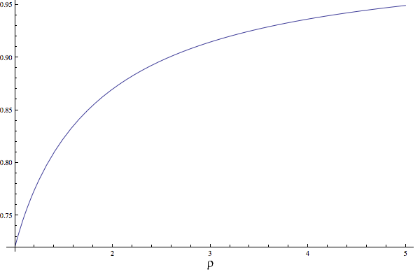
ϕ⁡(ρ):=limd→∞αℝ​(d,ρ​d)=∫(1−1ρ)2(1+1ρ)2x​12​π​((1+1ρ)2−x)​(x−(1−1ρ)2)1ρ​x​𝑑x.\phi(\rho):=\lim_{d\to\infty}\alpha_{\mathbb{R}}(d,\rho d)=\int_{\left(1-\sqrt{\frac{1}{\rho}}\right)^{2}}^{\left(1+\sqrt{\frac{1}{\rho}}\right)^{2}}\sqrt{x}\frac{1}{2\pi}\frac{\sqrt{(\left(1+\sqrt{\frac{1}{\rho}}\right)^{2}-x)(x-\left(1-\sqrt{\frac{1}{\rho}}\right)^{2})}}{\frac{1}{\rho}x}dx.

Although we do not provide a closed form solution for ϕ⁡(ρ)\phi(\rho) the integral can be easily computed numerically and we plot it below. It shows how the approximation ratio improves as ρ\rho increases.

Refer to caption
Figure 2: Plot of ϕ⁡(ρ)=limd→∞αℝ​(d,ρ​d)\phi(\rho)=\lim_{d\to\infty}\alpha_{\mathbb{R}}(d,\rho d) for ρ∈[1,5]\rho\in[1,5].

6 Integrality Gap

In this section we provide an integrality gap for relaxation (5) that matches our approximation ratio αℝ​(d)2\alpha_{\mathbb{R}}(d)^{2}. For the sake of the exposition we will restrict ourselves to the real case, but it is not difficult to see that all the arguments can be adapted to the complex case.

Our construction is an adaption of the classical construction for the d=1d=1 case (see, e.g., [AN04]). As it will become clear below, there is an extra difficulty in the d>1d>1 orthogonal case. In fact, the bound on the integrality gap of (5) given by this construction is αℝ∗​(d)2\alpha_{\mathbb{R}}^{\ast}(d)^{2}, defined as

αℝ∗​(d)=maxD​ diagonal‖D‖F2=d,D⪰0⁡𝔼​1d​∑i=1dσi​(G​D),\alpha_{\mathbb{R}}^{\ast}(d)=\max_{\begin{subarray}{c}D\text{ diagonal}\\ \|D\|_{F}^{2}=d,\ D\succeq 0\end{subarray}}\mathbb{E}\frac{1}{d}\sum_{i=1}^{d}\sigma_{i}(GD), (21)

where GG is a Gaussian matrix with i.i.d. real entries 𝒩⁡(0,1d)\mathcal{N}\left(0,\frac{1}{d}\right).

Fortunately, using the notion of operator concavity of a function and the Lowner-Heinz Theorem [Car09], we are able to show the following Theorem.

Theorem 13

Let d≥1d\geq 1. Also, let αℝ​(d)\alpha_{\mathbb{R}}(d) be as defined in Definition 2 and αℝ∗​(d)\alpha_{\mathbb{R}}^{\ast}(d) as defined in (21). Then,

αℝ∗​(d)=αℝ​(d).\alpha_{\mathbb{R}}^{\ast}(d)=\alpha_{\mathbb{R}}(d).

Proof. We want to show that

maxD​ diagonal‖D‖F2=dD⪰0⁡𝔼​∑i=1σi​(G​D)=𝔼​∑i=1σi​(G),\max_{\begin{subarray}{c}D\text{ diagonal}\\ \|D\|_{F}^{2}=d\\ D\succeq 0\end{subarray}}\mathbb{E}\sum_{i=1}\sigma_{i}(GD)=\mathbb{E}\sum_{i=1}\sigma_{i}(G),

where GG is a d×dd\times d matrix with i.i.d. entries 𝒩⁡(0,1d)\mathcal{N}\left(0,\frac{1}{d}\right). By taking V=D2V=D^{2}, and recalling the definition of singular value, we obtain the following claim (which immediately implies Theorem 13)

Claim 6.1
maxV​ diagonaltr⁡(V)=dV⪰0⁡𝔼​tr⁡[(G​V​GT)12]=𝔼​tr⁡[(G​GT)12].\max_{\begin{subarray}{c}V\text{ diagonal}\\ \operatorname{tr}(V)=d\\ V\succeq 0\end{subarray}}\mathbb{E}\operatorname{tr}\left[\left(GVG^{T}\right)^{\frac{1}{2}}\right]=\mathbb{E}\operatorname{tr}\left[\left(GG^{T}\right)^{\frac{1}{2}}\right].

Proof. We will proceed by contradiction, suppose (6.1) does not hold. Since the optimization space is compact and the function continuous it must have a maximum that is attained by a certain V≠Id×dV\neq I_{d\times d}. Out of all maximizers VV, let V(∗)V^{(\ast)} be the one with smallest possible Frobenius norm. The idea will be to use concavity arguments to build an optimal V(card)V^{({\rm card})} with smaller Frobenius norm, arriving at a contradiction and hence showing the theorem.

Since V(∗)V^{(\ast)} is optimal we have

𝔼​tr⁡[(G​V(∗)​GT)12]=αℝ∗​(d).\mathbb{E}\operatorname{tr}\left[\left(GV^{(\ast)}G^{T}\right)^{\frac{1}{2}}\right]=\alpha_{\mathbb{R}}^{\ast}(d).

Furthermore, since V(∗)≠Id×dV^{(\ast)}\neq I_{d\times d}, it must have two different diagonal elements. Let V(∗∗)V^{(\ast\ast)} be a matrix obtained by swapping, in V(∗)V^{(\ast)}, two of its non-equal diagonal elements. Clearly, ∥V(∗∗)∥F=∥V(∗)∥F\|V^{(\ast\ast)}\|_{F}=\|V^{(\ast)}\|_{F} and, because of the rotation invariance of the Gaussian, it is easy to see that

𝔼tr[(GV(∗∗)GT)12]=αℝ∗(d).\mathbb{E}\operatorname{tr}\left[\left(GV^{(\ast\ast)}G^{T}\right)^{\frac{1}{2}}\right]=\alpha_{\mathbb{R}}^{\ast}(d).

Since V(∗)⪰0V^{(\ast)}\succeq 0, these two matrices are not multiples of each other and so

V(card)=V(∗)+V(∗∗)2,V^{({\rm card})}=\frac{V^{(\ast)}+V^{(\ast\ast)}}{2},

has a strictly smaller Frobenius norm than V(∗)V^{(\ast)}. It is also clear that V(card)V^{({\rm card})} is a feasible solution. We conclude the proof by showing

𝔼tr[(GV(card)GT)12]≥12(𝔼tr[(GV(∗)GT)12]+𝔼tr[(GV(∗∗)GT)12])=αℝ∗(d).\mathbb{E}\operatorname{tr}\left[\left(GV^{({\rm card})}G^{T}\right)^{\frac{1}{2}}\right]\geq\frac{1}{2}\left(\mathbb{E}\operatorname{tr}\left[\left(GV^{(\ast)}G^{T}\right)^{\frac{1}{2}}\right]+\mathbb{E}\operatorname{tr}\left[\left(GV^{(\ast\ast)}G^{T}\right)^{\frac{1}{2}}\right]\right)=\alpha_{\mathbb{R}}^{\ast}(d). (22)

By linearity of expectation and construction of V(card)V^{({\rm card})}, (22) is equivalent to

𝔼[tr[(GV(∗)GT+GV(∗∗)GT2)12]−12(tr[(GV(∗)GT)12]+tr[(GV(∗∗)GT)12])]≥0.\mathbb{E}\left[\operatorname{tr}\left[\left(\frac{GV^{(\ast)}G^{T}+GV^{(\ast\ast)}G^{T}}{2}\right)^{\frac{1}{2}}\right]-\frac{1}{2}\left(\operatorname{tr}\left[\left(GV^{(\ast)}G^{T}\right)^{\frac{1}{2}}\right]+\operatorname{tr}\left[\left(GV^{(\ast\ast)}G^{T}\right)^{\frac{1}{2}}\right]\right)\right]\geq 0.

This inequality follows from the stronger statement: Given two d×dd\times d matrices A⪰0A\succeq 0 and B⪰0B\succeq 0, the following holds

(A+B2)12−A12+B122⪰0.\left(\frac{A+B}{2}\right)^{\frac{1}{2}}-\frac{A^{\frac{1}{2}}+B^{\frac{1}{2}}}{2}\succeq 0. (23)

Finally, (23) follows from the Lowner-Heinz Theorem, which states that the square root function is operator concave (See these lecture notes [Car09] for a very nice introduction to these inequalities).

Theorem 13 guarantees the optimality of the approximation ratio obtained in Section 3. In fact, we show the theorem below.

Theorem 14

For any d≥1d\geq 1 and any ε>0\varepsilon>0, there exists nn for which there exists C∈ℝd​n×d​nC\in\mathbb{R}^{dn\times dn} such that C⪰0C\succeq 0, and

maxO1,…,On∈𝒪d∑i=1n∑j=1ntr(Ci​jTOiOjT)maxXi​XiT=Id×dXi∈ℝd×d​n∑i=1n∑j=1ntr(Ci​jTXiXjT)≤αℝ​(d)2+ε.\frac{\displaystyle{\max_{O_{1},...,O_{n}\in\mathcal{O}_{d}}\sum_{i=1}^{n}\sum_{j=1}^{n}\operatorname{tr}\left(C_{ij}^{T}O_{i}O_{j}^{T}\right)}}{\displaystyle{\max_{\begin{subarray}{c}X_{i}X_{i}^{T}=I_{d\times d}\\ X_{i}\in\mathbb{R}^{d\times dn}\end{subarray}}\sum_{i=1}^{n}\sum_{j=1}^{n}\operatorname{tr}\left(C_{ij}^{T}X_{i}X_{j}^{T}\right)}}\leq\alpha_{\mathbb{R}}(d)^{2}+\varepsilon. (24)

We will construct CC randomly and show that it satisfies (24) with positive probability. Given pp an integer we consider nn i.i.d. matrix random variables VkV_{k}, with k=1,…,nk=1,\dots,n, where each VkV_{k} is a d×d​pd\times dp Gaussian matrix whose entries are 𝒩⁡(0,1d​p)\mathcal{N}(0,\frac{1}{dp}). We then define CC as the random matrix with d×dd\times d blocks Ci​j=1n2​Vi​VjTC_{ij}=\frac{1}{n^{2}}V_{i}V_{j}^{T}. The idea now is to understand the typical behavior of both

wr=maxXi​XiT=Id×dXi∈ℝd×d​n∑i=1n∑j=1ntr(Ci​jTXiXjT) and wc=maxO1,…,On∈𝒪d∑i=1n∑j=1ntr(Ci​jTOiOjT).w_{r}=\max_{\begin{subarray}{c}X_{i}X_{i}^{T}=I_{d\times d}\\ X_{i}\in\mathbb{R}^{d\times dn}\end{subarray}}\sum_{i=1}^{n}\sum_{j=1}^{n}\operatorname{tr}\left(C_{ij}^{T}X_{i}X_{j}^{T}\right)\text{ and }w_{c}=\max_{O_{1},...,O_{n}\in\mathcal{O}_{d}}\sum_{i=1}^{n}\sum_{j=1}^{n}\operatorname{tr}\left(C_{ij}^{T}O_{i}O_{j}^{T}\right).

For wcw_{c}, we can rewrite

wc=maxO1,…,On∈𝒪d⁡1n2​∑i,jtr⁡((Vi​VjT)T​Oi​OjT)=maxO1,…,On∈𝒪d⁡‖1n​∑i=1nOiT​Vi‖F2.w_{c}=\max_{O_{1},...,O_{n}\in\mathcal{O}_{d}}\frac{1}{n^{2}}\sum_{i,j}\operatorname{tr}\left((V_{i}V_{j}^{T})^{T}O_{i}O_{j}^{T}\right)=\max_{O_{1},...,O_{n}\in\mathcal{O}_{d}}\left\|\frac{1}{n}\sum_{i=1}^{n}O_{i}^{T}V_{i}\right\|_{F}^{2}.

If 𝒟=1n​∑i=1nOiT​Vi‖1n​∑i=1nOiT​Vi‖F\mathcal{D}=\frac{\frac{1}{n}\sum_{i=1}^{n}O_{i}^{T}V_{i}}{\left\|\frac{1}{n}\sum_{i=1}^{n}O_{i}^{T}V_{i}\right\|_{F}} then wc=∑i=1ntr⁡(maxOi∈𝒪d⁡OiT​Vi​𝒟T)=∑i=1ntr⁡(𝒫​(Vi​𝒟T)T​Vi​𝒟T)\sqrt{w_{c}}=\sum_{i=1}^{n}\operatorname{tr}\left(\max_{O_{i}\in\mathcal{O}_{d}}O_{i}^{T}V_{i}\mathcal{D}^{T}\right)=\sum_{i=1}^{n}\operatorname{tr}\left(\mathcal{P}(V_{i}\mathcal{D}^{T})^{T}V_{i}\mathcal{D}^{T}\right). The idea is that, given a fixed (direction unit frobenius-norm matrix) 𝒟\mathcal{D}, ∑i=1ntr⁡(𝒫​(Vi​𝒟T)T​Vi​𝒟T)\sum_{i=1}^{n}\operatorname{tr}\left(\mathcal{P}(V_{i}\mathcal{D}^{T})^{T}V_{i}\mathcal{D}^{T}\right) converges to the expected value of one of the summands and, by an ϵ\epsilon-net argument (since the dimension of the space where 𝒟\mathcal{D} is depends only on dd and pp and the number of summands is nn which can be made much larger than dd and pp) we can argue that the sum is close, for all 𝒟\mathcal{D}’s simultaneously, to that expectation. It is not hard to see that we can assume that 𝒟=1d​[D​ 0]\mathcal{D}=\frac{1}{\sqrt{d}}[D\ 0] where DD is diagonal and non-negative d×dd\times d matrix with ‖D‖F2=d\|D\|_{F}^{2}=d. In that case (see (21)),

𝔼​tr⁡(𝒫​(Vi​𝒟T)T​Vi​𝒟T)=𝔼​1p​d​∑k=1dσk​(G​D)≤dp​αℝ∗​(d),\mathbb{E}\operatorname{tr}\left(\mathcal{P}(V_{i}\mathcal{D}^{T})^{T}V_{i}\mathcal{D}^{T}\right)=\mathbb{E}\frac{1}{\sqrt{pd}}\sum_{k=1}^{d}\sigma_{k}(GD)\leq\sqrt{\frac{d}{p}}\alpha_{\mathbb{R}}^{\ast}(d),

where GG is a Gaussian matrix with i.i.d. real entries 𝒩⁡(0,1d)\mathcal{N}\left(0,\frac{1}{d}\right). This, together with Theorem 13, gives 𝔼​tr⁡(𝒫​(Vi​𝒟T)T​Vi​𝒟T)≤dp​αℝ​(d)\mathbb{E}\operatorname{tr}\left(\mathcal{P}(V_{i}\mathcal{D}^{T})^{T}V_{i}\mathcal{D}^{T}\right)\leq\sqrt{\frac{d}{p}}\alpha_{\mathbb{R}}(d). All of this is made precise in the following lemma

Lemma 15

For any dd and ε>0\varepsilon>0 there exists p0p_{0} and n0n_{0} such that, for any p>p0p>p_{0} and n>n0n>n_{0},

maxO1,…,On∈𝒪d⁡‖1n​∑i=1nOiT​Vi‖F2≤dp​αℝ​(d)2+ε,\max_{O_{1},...,O_{n}\in\mathcal{O}_{d}}\left\|\frac{1}{n}\sum_{i=1}^{n}O_{i}^{T}V_{i}\right\|_{F}^{2}\leq\frac{d}{p}\alpha_{\mathbb{R}}(d)^{2}+\varepsilon,

with probability strictly larger than 1/21/2.

Proof. Let us define

A⁡(V):=maxO1,…,On∈𝒪d⁡‖1n​∑i=1nOiT​Vi‖F.A(V):=\max_{O_{1},...,O_{n}\in\mathcal{O}_{d}}\left\|\frac{1}{n}\sum_{i=1}^{n}O_{i}^{T}V_{i}\right\|_{F}.

We have

A⁡(V)\displaystyle A(V) =\displaystyle= maxD∈ℝd×p​d:‖D‖F=1maxO1,…,On∈O⁡(d)tr(1n∑i=1nOiTViDT)\displaystyle\max_{D\in\mathbb{R}^{d\times pd}:\|D\|_{F}=1}\max_{O_{1},...,O_{n}\in O(d)}\operatorname{tr}\left(\frac{1}{n}\sum_{i=1}^{n}O_{i}^{T}V_{i}D^{T}\right)
=\displaystyle= maxD∈ℝd×p​d:‖D‖F=11n∑i=1nmaxOi∈O⁡(d)tr(OiTViDT)\displaystyle\max_{D\in\mathbb{R}^{d\times pd}:\|D\|_{F}=1}\frac{1}{n}\sum_{i=1}^{n}\max_{O_{i}\in O(d)}\operatorname{tr}\left(O_{i}^{T}V_{i}D^{T}\right)
=\displaystyle= maxD∈ℝd×p​d:‖D‖F=11n∑i=1ntr(𝒫(ViDT)TViDT).\displaystyle\max_{D\in\mathbb{R}^{d\times pd}:\|D\|_{F}=1}\frac{1}{n}\sum_{i=1}^{n}\operatorname{tr}\left(\mathcal{P}\left(V_{i}D^{T}\right)^{T}V_{i}D^{T}\right).

For DD with ‖D‖F=1\|D\|_{F}=1, we define

AD​(V)=1n​∑i=1ntr⁡(𝒫​(Vi​DT)T​Vi​DT).A_{D}(V)=\frac{1}{n}\sum_{i=1}^{n}\operatorname{tr}\left(\mathcal{P}\left(V_{i}D^{T}\right)^{T}V_{i}D^{T}\right).

We proceed by understanding the behavior of AD​(V)A_{D}(V) for a specific DD.

Let D=UL​[Σ​ 0]​URTD=U_{L}[\Sigma\ 0]U_{R}^{T}, where Σ\Sigma is a d×dd\times d non-negative diagonal matrix, be the singular value decomposition of DD. For each i=1,…,ni=1,\dots,n, we have (using rotation invariance of the Gaussian distribution):

tr⁡(𝒫​(Vi​DT)T​Vi​DT)\displaystyle\operatorname{tr}\left(\mathcal{P}\left(V_{i}D^{T}\right)^{T}V_{i}D^{T}\right) ∼\displaystyle\sim tr⁡(𝒫​(Vi​(UL​[Σ​ 0]​UR)T)T​Vi​(UL​[Σ​ 0]​UR)T)\displaystyle\operatorname{tr}\left(\mathcal{P}\left(V_{i}(U_{L}[\Sigma\ 0]U_{R})^{T}\right)^{T}V_{i}(U_{L}[\Sigma\ 0]U_{R})^{T}\right)
∼\displaystyle\sim tr⁡(UL​𝒫​(Vi​[Σ0])T​Vi​[Σ0]​ULT)\displaystyle\operatorname{tr}\left(U_{L}\mathcal{P}\left(V_{i}\left[\begin{subarray}{c}\Sigma\\ 0\end{subarray}\right]\right)^{T}V_{i}\left[\begin{subarray}{c}\Sigma\\ 0\end{subarray}\right]U_{L}^{T}\right)
∼\displaystyle\sim tr⁡(𝒫​(Vi​[Σ0])T​Vi​[Σ0])\displaystyle\operatorname{tr}\left(\mathcal{P}\left(V_{i}\left[\begin{subarray}{c}\Sigma\\ 0\end{subarray}\right]\right)^{T}V_{i}\left[\begin{subarray}{c}\Sigma\\ 0\end{subarray}\right]\right)
∼\displaystyle\sim 1d​p​tr⁡(𝒫​(G​d​Σ)T​G​d​Σ),\displaystyle\frac{1}{\sqrt{dp}}\operatorname{tr}\left(\mathcal{P}\left(G\sqrt{d}\Sigma\right)^{T}G\sqrt{d}\Sigma\right),

where GG is a d×dd\times d Gaussian matrix with 𝒩⁡(0,1d)\mathcal{N}(0,\frac{1}{d}) entries.

This means that

AD​(V)=1n​∑i=1nXi,A_{D}(V)=\frac{1}{n}\sum_{i=1}^{n}X_{i},

with XiX_{i} i.i.d. distributed as 1d​p​tr⁡(𝒫​(G​d​Σ)T​G​d​Σ)\frac{1}{\sqrt{dp}}\operatorname{tr}\left(\mathcal{P}\left(G\sqrt{d}\Sigma\right)^{T}G\sqrt{d}\Sigma\right).

Since ‖d​Σ‖F2=d\|\sqrt{d}\Sigma\|_{F}^{2}=d, by (21), we get

𝔼​tr⁡(𝒫​(G​d​Σ)T​G​d​Σ)≤d​αℝ∗​(d).\mathbb{E}\operatorname{tr}\left(\mathcal{P}\left(G\sqrt{d}\Sigma\right)^{T}G\sqrt{d}\Sigma\right)\leq d\alpha_{\mathbb{R}}^{\ast}(d).

This, together with Theorem 13, gives

𝔼​Xi≤dp​αℝ​(d).\mathbb{E}X_{i}\leq\sqrt{\frac{d}{p}}\alpha_{\mathbb{R}}(d). (25)

In order to give tail bounds for AD​(V)=1n​∑i=1nXiA_{D}(V)=\frac{1}{n}\sum_{i=1}^{n}X_{i} we will show that XiX_{i} is subgaussian and use Hoeffding’s inequality (see Vershynin’s notes [Ver12]). In fact,

Xi∼1d​p​tr⁡(𝒫​(G​d​Σ)T​G​d​Σ)≤1p​‖𝒫⁡(G​Σ)‖F​‖G​Σ‖F=dp​‖G​D‖F≤dp​‖G‖F.X_{i}\sim\frac{1}{\sqrt{dp}}\operatorname{tr}\left(\mathcal{P}\left(G\sqrt{d}\Sigma\right)^{T}G\sqrt{d}\Sigma\right)\leq\frac{1}{\sqrt{p}}\|\mathcal{P}\left(G\Sigma\right)\|_{F}\|G\Sigma\|_{F}=\sqrt{\frac{d}{p}}\|GD\|_{F}\leq\sqrt{\frac{d}{p}}\|G\|_{F}.

Note that dp​‖G‖F\sqrt{\frac{d}{p}}\|G\|_{F} is a subgaussian random variable as ‖G‖F\|G\|_{F} is smaller than the entry wise ℓ1\ell_{1} norm of GG which is the sum of d2d^{2} half-normals (more specifically, the absolute value of a 𝒩⁡(0,1d)\mathcal{N}(0,\frac{1}{d}) random variable). Since half-normals are subgaussian and the sum of subgaussian random variables is a subgaussian random variable with subgaussian norm at most the sum of the norms (see the Rotation invariance Lemma in [Ver12]) we get that XiX_{i} is subgaussian. Furthermore, the subgaussian norm of XiX_{i}, which we define as ∥Xi∥ψ2=supp≥1p−1/2(𝔼|X|p)1/p\|X_{i}\|_{\psi_{2}}=\sup_{p\geq 1}p^{-1/2}(\mathbb{E}|X|^{p})^{1/p}, is bounded by ‖Xi‖ψ2≤C​d2p=C​dp\|X_{i}\|_{\psi_{2}}\leq C\sqrt{\frac{d^{2}}{p}}=C\frac{d}{\sqrt{p}}, for some universal constant CC.

Hence, we can use Hoeffding’s inequality (see [Ver12]) and get, since 𝔼​Xi≤dp​αℝ​(d)\mathbb{E}X_{i}\leq\sqrt{\frac{d}{p}}\alpha_{\mathbb{R}}(d),

Prob[AD≥dpαℝ(d)+t]≤Prob[|AD−𝔼Xi|≥t]≤exp(1−c2​t2​n‖Xi‖ψ22)≤3exp(−c1t2​pd2n),\mathrm{Prob}\left[A_{D}\geq\sqrt{\frac{d}{p}}\alpha_{\mathbb{R}}(d)+t\right]\leq\mathrm{Prob}\left[\left|A_{D}-\mathbb{E}X_{i}\right|\geq t\right]\leq\exp\left(1-\frac{c_{2}t^{2}n}{\|X_{i}\|_{\psi_{2}}^{2}}\right)\leq 3\exp\left(-c_{1}\frac{t^{2}p}{d^{2}}n\right),

where cic_{i} are universal constants.

To find an upper bound for A=maxD∈ℝd×p​d:‖D‖F=1ADA=\max_{D\in\mathbb{R}^{d\times pd}:\|D\|_{F}=1}A_{D} we use a classicl ϵ\epsilon-net argument. There exists a set 𝒩\mathcal{N} of matrices Dk∈ℝd×p​dD_{k}\in\mathbb{R}^{d\times pd} satisfying ‖Dk‖F=1\|D_{k}\|_{F}=1, such that for any D∈ℝd×p​dD\in\mathbb{R}^{d\times pd} with Frobenius norm 11, there exists an element Dk∈𝒩D_{k}\in\mathcal{N} such that ‖D−Dk‖F≤ϵ||D-D_{k}||_{F}\leq\epsilon. 𝒩\mathcal{N} is called an ϵ\epsilon-net, and it’s known (see [Ver12]) that there exists such a set with size

|𝒩|≤(1+2ϵ)d2​p.|\mathcal{N}|\leq\left(1+\frac{2}{\epsilon}\right)^{d^{2}p}.

By the union-bound, with probability at least

1−|𝒩|Prob[AD≥dpαℝ(d)+t]≥1−[(1+2ϵ)d2​p3exp(−c1t2​nd3)],1-|\mathcal{N}|\,\mathrm{Prob}\left[A_{D}\geq\sqrt{\frac{d}{p}}\alpha_{\mathbb{R}}(d)+t\right]\geq 1-\left[\left(1+\frac{2}{\epsilon}\right)^{d^{2}p}3\exp\left(-c_{1}\frac{t^{2}n}{d^{3}}\right)\right],

all the DkD_{k}’s in 𝒩\mathcal{N} satisfy

ADk≤dp​αℝ∗​(d)+t.A_{D_{k}}\leq\sqrt{\frac{d}{p}}\alpha_{\mathbb{R}}^{\ast}(d)+t.

If DD is not in 𝒩\mathcal{N}, there exists Dk∈𝒩D_{k}\in\mathcal{N} such that ‖D−Dk‖F≤ϵ\|D-D_{k}\|_{F}\leq\epsilon. This means that

AD\displaystyle A_{D} ≤\displaystyle\leq 1n​∑i=1ntr⁡(𝒫​(Vi​DT)T​Vi​D∗T)+1n​∑i=1ntr⁡(𝒫​(Vi​DT)T​Vi​(D∗T−DT))\displaystyle\frac{1}{n}\sum_{i=1}^{n}\operatorname{tr}\left(\mathcal{P}\left(V_{i}D^{T}\right)^{T}V_{i}D_{\ast}^{T}\right)+\frac{1}{n}\sum_{i=1}^{n}\operatorname{tr}\left(\mathcal{P}\left(V_{i}D^{T}\right)^{T}V_{i}(D_{\ast}^{T}-D^{T})\right)
≤\displaystyle\leq 1n​∑i=1ntr⁡(𝒫​(Vi​D∗T)T​Vi​D∗T)+1n​∑i=1n‖𝒫​(Vi​DT)T​Vi‖F​‖D∗−D‖F\displaystyle\frac{1}{n}\sum_{i=1}^{n}\operatorname{tr}\left(\mathcal{P}\left(V_{i}D_{\ast}^{T}\right)^{T}V_{i}D_{\ast}^{T}\right)+\frac{1}{n}\sum_{i=1}^{n}\|\mathcal{P}\left(V_{i}D^{T}\right)^{T}V_{i}\|_{F}\|D_{\ast}-D\|_{F}
≤\displaystyle\leq dp​αℝ∗​(d)+t+ϵ⁡(1n​∑i=1n‖Vi‖F).\displaystyle\sqrt{\frac{d}{p}}\alpha_{\mathbb{R}}^{\ast}(d)+t+\epsilon\left(\frac{1}{n}\sum_{i=1}^{n}\|V_{i}\|_{F}\right).

We can globally bound (1n​∑i=1n‖Vi‖F)\left(\frac{1}{n}\sum_{i=1}^{n}\|V_{i}\|_{F}\right) by Hoeffding’s inequality as well (see [Ver12]). Using the same argument as above, it is easy to see that ‖Vi‖F\|V_{i}\|_{F} has subgaussian norm bounded by d\sqrt{d}, and an explicit computation shows its mean is 1d​p​2​Γ⁡((d2​p+1)/2)Γ⁡(d2​p/2)≤2​d\frac{1}{\sqrt{dp}}\sqrt{2}\frac{\Gamma((d^{2}p+1)/2)}{\Gamma(d^{2}p/2)}\leq 2\sqrt{d}, where the inequality follows from lemma 20.

This means that by Hoeffding’s inequality (see [Ver12])

Prob[1n∑i=1n∥Vi∥F≥2d+t]\displaystyle\mathrm{Prob}\left[\frac{1}{n}\sum_{i=1}^{n}\|V_{i}\|_{F}\geq 2\sqrt{d}+t\right] ≤\displaystyle\leq exp⁡(1−c4​t2​n‖‖Vi‖F‖ψ22)\displaystyle\exp\left(1-\frac{c_{4}t^{2}n}{\|\|V_{i}\|_{F}\|_{\psi_{2}}^{2}}\right)
≤\displaystyle\leq 3​exp⁡(−c3​t2​nd),\displaystyle 3\exp\left(-c_{3}\frac{t^{2}n}{d}\right),

with cic_{i} universal constants.

By union-bound on the two events above, with probability at least

1−3​exp⁡(−c3​t2​nd)−[(1+2ϵ)d2​p​3​exp⁡(−c1​t2​nd3)],1-3\exp\left(-c_{3}\frac{t^{2}n}{d}\right)-\left[\left(1+\frac{2}{\epsilon}\right)^{d^{2}p}3\exp\left(-c_{1}\frac{t^{2}n}{d^{3}}\right)\right],

we have

A≤dp​αℝ∗​(d)+t+ϵ⁡(2​d+t).A\leq\sqrt{\frac{d}{p}}\alpha_{\mathbb{R}}^{\ast}(d)+t+\epsilon(2d+t).

Choosing t=12​pt=\frac{1}{2p} and ϵ=16​d​p\epsilon=\frac{1}{6dp} we get

A≤dp​αℝ∗​(d)+1p,A\leq\sqrt{\frac{d}{p}}\alpha_{\mathbb{R}}^{\ast}(d)+\frac{1}{p},

with probability at least

1−3​exp⁡(−c3​n4​p2)−[(1+12​d​p)d2​p​3​exp⁡(−c1​n4​p2​d3)]\displaystyle 1-3\exp\left(-c_{3}\frac{n}{4p^{2}}\right)-\left[\left(1+12dp\right)^{d^{2}p}3\exp\left(-c_{1}\frac{n}{4p^{2}d^{3}}\right)\right]
=\displaystyle= 1−6​[(1+12​d​p)d2​p​3​exp⁡(−c1​n4​p2​d3)]\displaystyle 1-6\left[\left(1+12dp\right)^{d^{2}p}3\exp\left(-c_{1}\frac{n}{4p^{2}d^{3}}\right)\right]

which can be made arbitrarily close to 11 by taking nn large enough.

This means that

maxO1,…,On∈𝒪d⁡‖1n​∑i=1nOiT​Vi‖F2≤dp​αℝ​(d)2+1p,\max_{O_{1},...,O_{n}\in\mathcal{O}_{d}}\left\|\frac{1}{n}\sum_{i=1}^{n}O_{i}^{T}V_{i}\right\|_{F}^{2}\leq\frac{d}{p}\alpha_{\mathbb{R}}(d)^{2}+\frac{1}{p},

with high probability, proving the lemma. □\hfill\square

Regarding wrw_{r}, we know that it is at least the value of 1n2​∑i,jntr⁡((Vi​VjT)T​Xi​XjT)\frac{1}{n^{2}}\sum_{i,j}^{n}\operatorname{tr}\left((V_{i}V_{j}^{T})^{T}X_{i}X_{j}^{T}\right) for Xi=𝒫⁡(Vi)X_{i}=\mathcal{P}(V_{i}). Since, for pp large enough, Vi​ViT≈Id×dV_{i}V_{i}^{T}\approx I_{d\times d} we essentially have wr≳1n2​∑i,jn‖Vi​VjT‖F2w_{r}\gtrsim\frac{1}{n^{2}}\sum_{i,j}^{n}\|V_{i}V_{j}^{T}\|_{F}^{2} which should approximate 𝔼​‖Vi​VjT‖F2≈dp\mathbb{E}\|V_{i}V_{j}^{T}\|_{F}^{2}\approx\frac{d}{p}. This is made precise in the following lemma:

Lemma 16

For any dd and ε>0\varepsilon>0 there exists p0p_{0} and n0n_{0} such that, for any p>p0p>p_{0} and n>n0n>n_{0},

1n2​∑i,jntr⁡((Vi​VjT)T​𝒫(d,d​p)​(Vi)​𝒫(d,d​p)​(Vj)T)≥dp−ε,\frac{1}{n^{2}}\sum_{i,j}^{n}\operatorname{tr}\left((V_{i}V_{j}^{T})^{T}\mathcal{P}_{(d,dp)}(V_{i})\mathcal{P}_{(d,dp)}(V_{j})^{T}\right)\geq\frac{d}{p}-\varepsilon,

with probability strictly larger than 1/21/2.

Proof. Recall that 𝒫(d,d​p)​(Vi)\mathcal{P}_{(d,dp)}(V_{i}) is the d×d​pd\times dp matrix polar component of ViV_{i}, meaning that

tr⁡(𝒫(d,d​p)​(Vi)T​Vi)=∑k=1dσk​(Vi).\operatorname{tr}\left(\mathcal{P}_{(d,dp)}(V_{i})^{T}V_{i}\right)=\sum_{k=1}^{d}\sigma_{k}(V_{i}).

Hence,

1n2​∑i,jntr⁡((Vi​VjT)T​𝒫(d,d​p)​(Vi)​𝒫(d,d​p)​(Vj)T)\displaystyle\frac{1}{n^{2}}\sum_{i,j}^{n}\operatorname{tr}\left((V_{i}V_{j}^{T})^{T}\mathcal{P}_{(d,dp)}(V_{i})\mathcal{P}_{(d,dp)}(V_{j})^{T}\right) =\displaystyle= ‖1n​∑i=1n𝒫​(Vi)T​Vi‖F2\displaystyle\left\|\frac{1}{n}\sum_{i=1}^{n}\mathcal{P}(V_{i})^{T}V_{i}\right\|_{F}^{2}
≥\displaystyle\geq 1‖Id​p×d​p‖F2​[1n​∑i=1ntr⁡(𝒫​(Vi)T​Vi​Id​p×d​p)]2\displaystyle\frac{1}{\left\|I_{dp\times dp}\right\|_{F}^{2}}\left[\frac{1}{n}\sum_{i=1}^{n}\operatorname{tr}\left(\mathcal{P}(V_{i})^{T}V_{i}I_{dp\times dp}\right)\right]^{2}
=\displaystyle= 1d​p​[1n​∑i=1n∑k=1dσk​(Vi)]2.\displaystyle\frac{1}{dp}\left[\frac{1}{n}\sum_{i=1}^{n}\sum_{k=1}^{d}\sigma_{k}(V_{i})\right]^{2}.

We proceed by using a lower bound for the expected value of the smallest eigenvalue (see [Ver12]), and get

𝔼​∑k=1dσk​(Vi)≥d​𝔼​σmin​(Vi)=d⁡(1−1p).\mathbb{E}\sum_{k=1}^{d}\sigma_{k}(V_{i})\geq d\ \mathbb{E}\sigma_{\min}(V_{i})=d\left(1-\frac{1}{\sqrt{p}}\right).

Since ∑k=1dσk​(Vi)≤d​‖Vi‖F\sum_{k=1}^{d}\sigma_{k}(V_{i})\leq\sqrt{d}\|V_{i}\|_{F}, it has subgaussian norm smaller than C​dCd, with CC an universal constant (using the same argument as in Lemma 15). Therefore, by Hoeffding’s inequality (see [Ver12]),

Prob[1n∑i=1n∑k=1dσk(Vi)≤d(1−1p)−t]\displaystyle\mathrm{Prob}\left[\frac{1}{n}\sum_{i=1}^{n}\sum_{k=1}^{d}\sigma_{k}(V_{i})\leq d\left(1-\frac{1}{\sqrt{p}}\right)-t\right] ≤\displaystyle\leq exp⁡(1−c1​t2‖∑k=1dσk​(Vi)‖ψ22​n)\displaystyle\exp\left(1-\frac{c_{1}t^{2}}{\left\|\sum_{k=1}^{d}\sigma_{k}(V_{i})\right\|_{\psi_{2}}^{2}}n\right)
≤\displaystyle\leq exp⁡(1−c2​t2d2​n),\displaystyle\exp\left(1-c_{2}\frac{t^{2}}{d^{2}}n\right),

where cic_{i} are universal constants.

By setting t=dpt=\frac{d}{\sqrt{p}}, we get

1n2​∑i,jntr⁡((Vi​VjT)T​𝒫(d,d​p)​(Vi)​𝒫(d,d​p)​(Vj)T)≥dp​(1−2​1p)2,\frac{1}{n^{2}}\sum_{i,j}^{n}\operatorname{tr}\left((V_{i}V_{j}^{T})^{T}\mathcal{P}_{(d,dp)}(V_{i})\mathcal{P}_{(d,dp)}(V_{j})^{T}\right)\geq\frac{d}{p}\left(1-2\frac{1}{\sqrt{p}}\right)^{2},

with probability at least 1−exp⁡(1−c2​1p​n)=1−on​(1)1-\exp\left(1-c_{2}\frac{1}{p}n\right)=1-o_{n}(1), proving the Lemma. □\hfill\square

Theorem 14 immediately follows from these two lemmas.

We note that these techniques are quite general. It is not difficult to see that these arguments, establishing integrality gaps that match the approximation ratios obtained, can be easily adapted for both the unitary case and the rank constrained case introduced in Section 5. For the sake of exposition we omit the details in these cases.

7 Open Problems and Future Work

Besides Conjecture 8, there are several extensions of this work that the authors consider to be interesting directions for future work.

A natural extension is to consider the little Grothendieck problem (3) over other groups of matrices. One interesting extension would be to consider the special orthogonal group S​𝒪dS\mathcal{O}_{d} and the special unitary group S​𝒰dS\mathcal{U}_{d}, these seem more difficult since they are not described by quadratic constraints. 33 3 The additional constraint that forces a matrix to be in the special orthogonal or unitary group is having determinant equal to 11 which is not quadratic.

In some applications, like Synchronization [BSS13, Sin11] (a similar problem to Orthogonal Procrustes) and Common Lines [SS11], the positive semidefiniteness condition is not natural. It would be useful to better understand approximation algorithms for a version of (3) where CC is not assumed to be positive semidefinite. Previous work in the special case d=1d=1, [NRT99, CW04, AMMN05] for 𝒪1\mathcal{O}_{1} and [SZY07] for 𝒰1\mathcal{U}_{1}, suggest that it is possible to obtain an approximation ratio for (3) depending logarithmically on the size of the problem. Moreover, for 𝒪1\mathcal{O}_{1}, the logarithmic term is known to be needed in general [AMMN05].

It would also be interesting to understand whether the techniques in [AN04] can be adapted to obtain an approximation algorithm to the bipartite Grothendieck problem over the orthogonal group; this would be closer in spirit to the non commutative Grothendieck inequality [NRV13].

Another interesting question is whether the approximation ratios obtained in this paper correspond to the hardness of approximation of the problem (perhaps conditioned on the Unique-Games conjecture [Kho10]). Our optimality conditions are restricted to the particular relaxation we consider and do not exclude the existence of an efficient algorithm, not relying on the same relaxation, that approximates (3) with a better approximation ratio. Nevertheless, Raghavendra [Rag08] results on hardness for a host of problems matching the integrality gap of natural SDP relaxations suggest that our approximation ratios might be optimal (see also the recent results in [BRS15]).

Acknowledgments

The authors would like to thank Moses Charikar for valuable guidance in context of this work and Jop Briet, Alexander Iriza, Yuehaw Khoo, Dustin Mixon, Oded Regev, and Zhizhen Zhao for insightful discussions on the topic of this paper. Special thanks to Johannes Trost for a very useful answer to a Mathoverflow question posed by the first author. Finally, we would like to thank the reviewers for numerous suggestions that helped to greatly improve the quality of this paper.

A. S. Bandeira was supported by AFOSR Grant No. FA9550-12-1-0317. A. Singer was partially supported by Award Number FA9550-12-1-0317 and FA9550-13-1-0076 from AFOSR, by Award Number R01GM090200 from the NIGMS, and by Award Number LTR DTD 06-05-2012 from the Simons Foundation. Parts of this work have appeared in C. Kennedy’s senior thesis at Princeton University.

References

  • [AMMN05] N. Alon, K. Makarychev, Y. Makarychev, and A. Naor. Quadratic forms on graphs. Invent. Math, 163:486–493, 2005.
  • [AN04] N. Alon and A. Naor. Approximating the cut-norm via Grothendieck’s inequality. In Proc. of the 36 th ACM STOC, pages 72–80. ACM Press, 2004.
  • [AS64] M. Abramowitz and I. A. Stegun. Handbook of Mathematical Functions with Formulas, Graphs, and Mathematical Tables. Dover, New York, 1964.
  • [Ban15] A. S. Bandeira. Convex relaxations for certain inverse problems on graphs. PhD thesis, Program in Applied and Computational Mathematics, Princeton University, 2015.
  • [BBT11] J. Briet, H. Buhrman, and B. Toner. A generalized Grothendieck inequality and nonlocal correlations that require high entanglement. Communications in Mathematical Physics, 305(3):827–843, 2011.
  • [BFV10] J. Briet, F. M. O. Filho, and F. Vallentin. The positive semidefinite Grothendieck problem with rank constraint. In Automata, Languages and Programming, volume 6198 of Lecture Notes in Computer Science, pages 31–42. Springer Berlin Heidelberg, 2010.
  • [BRS15] J. Briet, O. Regev, and R. Saket. Tight hardness of the non-commutative Grothendieck problem. FOCS 2015, to appear, 2015.
  • [BSS13] A. S. Bandeira, A. Singer, and D. A. Spielman. A Cheeger inequality for the graph connection Laplacian. SIAM J. Matrix Anal. Appl., 34(4):1611–1630, 2013.
  • [BTN02] A. Ben-Tal and A. Nemirovski. On tractable approximations of uncertain linear matrix inequalities affected by interval uncertainty. SIAM Journal on Optimization, 12:811–833, 2002.
  • [Car09] E. A. Carlen. Trace inequalities and quantum entropy: An introductory course. available at http://www.ueltschi.org/azschool/notes/ericcarlen.pdf, 2009.
  • [CD11] R. Couillet and M. Debbah. Random Matrix Methods for Wireless Communications. Cambridge University Press, New York, NY, USA, 2011.
  • [CKS15] K. N. Chaudhury, Y. Khoo, and A. Singer. Global registration of multiple point clouds using semidefinite programming. SIAM Journal on Optimization, 25(1):126–185, 2015.
  • [CW04] M. Charikar and A. Wirth. Maximizing quadratic programs: Extending Grothendieck’s inequality. In Proceedings of the 45th Annual IEEE Symposium on Foundations of Computer Science, FOCS ’04, pages 54–60, Washington, DC, USA, 2004. IEEE Computer Society.
  • [FH55] K. Fan and A. J. Hoffman. Some metric inequalities in the space of matrices. Proceedings of the American Mathematical Society, 6(1):pp. 111–116, 1955.
  • [GR94] I. S. Gradshteyn and I. M. Ryzhik. Table of Integrals, Series, and Products, Fifth Edition. Academic Press, 5th edition, January 1994.
  • [Gro96] A. Grothendieck. Resume de la theorie metrique des produits tensoriels topologiques (french). Reprint of Bol. Soc. Mat. Sao Paulo, page 1�79, 1996.
  • [GT11] F. Gotze and A. Tikhomirov. On the rate of convergence to the Marchenko–Pastur distribution. arXiv:1110.1284 [math.PR], 2011.
  • [GW95] M. X. Goemans and D. P. Williamson. Improved apprximation algorithms for maximum cut and satisfiability problems using semidefine programming. Journal of the Association for Computing Machinery, 42:1115–1145, 1995.
  • [Hig86] N. J. Higham. Computing the polar decomposition – with applications. SIAM J. Sci. Stat. Comput., 7:1160–1174, October 1986.
  • [Kel75] J. B. Keller. Closest unitary, orthogonal and hermitian operators to a given operator. Mathematics Magazine, 48(4):pp. 192–197, 1975.
  • [Kho10] S. Khot. On the unique games conjecture (invited survey). In Proceedings of the 2010 IEEE 25th Annual Conference on Computational Complexity, CCC ’10, pages 99–121, Washington, DC, USA, 2010. IEEE Computer Society.
  • [Lev12] O. Leveque. Random matrices and communication systems: Wishart random matrices: marginal eigenvalue distribution. Available at: http://ipg.epfl.ch/~leveque/Matrix/, 2012.
  • [LV11] G. Livan and P. Vivo. Moments of Wishart-Laguerre and Jacobi ensembles of random matrices: application to the quantum transport problem in chaotic cavities. Acta Physica Polonica B, 42:1081, 2011.
  • [Nem07] A. Nemirovski. Sums of random symmetric matrices and quadratic optimization under orthogonality constraints. Math. Program., 109(2-3):283–317, 2007.
  • [Nes98] Y. Nesterov. Semidefinite relaxation and nonconvex quadratic optimization. Optimization Methods and Software, 9(1-3):141–160, 1998.
  • [NRT99] A. Nemirovski, C. Roos, and T. Terlaky. On maximization of quadratic form over intersection of ellipsoids with common center. Mathematical Programming, 86(3):463–473, 1999.
  • [NRV13] A. Naor, O. Regev, and T. Vidick. Efficient rounding for the noncommutative Grothendieck inequality. In Proceedings of the 45th annual ACM symposium on Symposium on theory of computing, STOC ’13, pages 71–80, New York, NY, USA, 2013. ACM.
  • [Pis11] G. Pisier. Grothendieck’s theorem, past and present. Bull. Amer. Math. Soc., 49:237�323, 2011.
  • [Rag08] P. Raghavendra. Optimal algorithms and inapproximability results for every CSP. In In Proc. 40 th ACM STOC, pages 245–254, 2008.
  • [Sch66] P. H. Schonemann. A generalized solution of the orthogonal procrustes problem. Psychometrika, 31(1):1–10, 1966.
  • [She01] J. Shen. On the singular values of gaussian random matrices. Linear Algebra and its Applications, 326(13):1 – 14, 2001.
  • [Sin11] A. Singer. Angular synchronization by eigenvectors and semidefinite programming. Appl. Comput. Harmon. Anal., 30(1):20 – 36, 2011.
  • [So11] A.-C. So. Moment inequalities for sums of random matrices and their applications in optimization. Mathematical Programming, 130(1):125–151, 2011.
  • [SS11] A. Singer and Y. Shkolnisky. Three-dimensional structure determination from common lines in Cryo-EM by eigenvectors and semidefinite programming. SIAM J. Imaging Sciences, 4(2):543–572, 2011.
  • [SZY07] A. So, J. Zhang, and Y. Ye. On approximating complex quadratic optimization problems via semidefinite programming relaxations. Math. Program. Ser. B, 2007.
  • [TV04] A. M. Tulino and S. Verdú. Random matrix theory and wireless communications. Commun. Inf. Theory, 1(1):1–182, June 2004.
  • [VB96] L. Vanderberghe and S. Boyd. Semidefinite programming. SIAM Review, 38:49–95, 1996.
  • [Ver12] R. Vershynin. Introduction to the non-asymptotic analysis of random matrices. Chapter 5 of: Compressed Sensing, Theory and Applications. Edited by Y. Eldar and G. Kutyniok. Cambridge University Press, 2012.
  • [WGS12] Z. Wen, D. Goldfarb, and K. Scheinberg. Block coordinate descent methods for semidefinite programming. In Handbook on Semidefinite, Conic and Polynomial Optimization, volume 166 of International Series in Operations Research & Management Science, pages 533–564. Springer US, 2012.

Appendix A Technical proofs - analysis of algorithm for the Stiefel Manifold setting

Lemma 17

Let r≥dr\geq d. Let GG be a d×rd\times r Gaussian random matrix with real valued i.i.d. 𝒩⁡(0,1r)\mathcal{N}\left(0,\frac{1}{r}\right) entries and let αℝ​(d,r)\alpha_{\mathbb{R}}(d,r) as defined in Definition 11. Then,

𝔼⁡(𝒫d,r​(G)​GT)=𝔼⁡(G​𝒫d,r​(G)T)=αℝ​(d,r)​Id×d.\mathbb{E}\left(\mathcal{P}_{d,r}(G)G^{T}\right)=\mathbb{E}\left(G\mathcal{P}_{d,r}(G)^{T}\right)=\alpha_{\mathbb{R}}(d,r)I_{d\times d}.

Furthermore, if GG is a d×rd\times r Gaussian random matrix with complex valued i.i.d. 𝒩⁡(0,1r)\mathcal{N}\left(0,\frac{1}{r}\right) entries and αℂ​(d,r)\alpha_{\mathbb{C}}(d,r) the analogous constant (Definition 11), then

𝔼⁡(𝒫d,r​(G)​GH)=𝔼⁡(G​𝒫d,r​(G)H)=αℂ​(d,r)​Id×d.\mathbb{E}\left(\mathcal{P}_{d,r}(G)G^{H}\right)=\mathbb{E}\left(G\mathcal{P}_{d,r}(G)^{H}\right)=\alpha_{\mathbb{C}}(d,r)I_{d\times d}.

The proof of this Lemma is a simple adaptation of the proof of Lemma 6.

Proof. We restrict the presentation to the real case. As before, all the arguments are equivalent to the complex case, replacing all transposes with Hermitian adjoints and αℝ​(d,r)\alpha_{\mathbb{R}}(d,r) with αℂ​(d,r)\alpha_{\mathbb{C}}(d,r).

Let G=U⁡[Σ​ 0]​VTG=U[\Sigma\ 0]V^{T} be the singular value decomposition of GG. Since G​GT=U​Σ2​UTGG^{T}=U\Sigma^{2}U^{T} is a Wishart matrix, it is well known that its eigenvalues and eigenvectors are independent and UU is distributed according to the Haar measure in 𝒪d\mathcal{O}_{d} (see e.g. Lemma 2.6 in [TV04]). To resolve ambiguities, we consider Σ\Sigma ordered such that Σ11≥Σ22≥…≥Σd​d\Sigma_{11}\geq\Sigma_{22}\geq...\geq\Sigma_{dd}.

Let Y=𝒫(d,r)​(G)​GTY=\mathcal{P}_{(d,r)}(G)G^{T}. Since

𝒫(d,r)​(G)=𝒫(d,r)​(U⁡[Σ​ 0]​VT)=U⁡[Id×d​ 0]​VT,\mathcal{P}_{(d,r)}(G)=\mathcal{P}_{(d,r)}(U[\Sigma\ 0]V^{T})=U[I_{d\times d}\ 0]V^{T},

we have

Y=𝒫(d,r)​(U⁡[Σ​ 0]​VT)​(U⁡[Σ​ 0]​VT)T=U⁡[Id×d​ 0]​VT​V​Σ​UT=U​Σ​UT.Y=\mathcal{P}_{(d,r)}(U[\Sigma\ 0]V^{T})(U[\Sigma\ 0]V^{T})^{T}=U[I_{d\times d}\ 0]V^{T}V\Sigma U^{T}=U\Sigma U^{T}.

Note that G​𝒫(d,r)​(G)T=U​Σ​UT=YG\mathcal{P}_{(d,r)}(G)^{T}=U\Sigma U^{T}=Y.

Since Yi​j=ui​Σ​ujTY_{ij}=u_{i}\Sigma u_{j}^{T}, where u1,…,udu_{1},\dots,u_{d} are the rows of UU, and UU is distributed according to the Haar measure, we have that uju_{j} and −uj-u_{j} have the same distribution conditioned on any uiu_{i}, for i≠ji\neq j, and Σ\Sigma. This implies that, if i≠ji\neq j, Yi​j=ui​Σ​ujTY_{ij}=u_{i}\Sigma u_{j}^{T} is a symmetric random variable, and so 𝔼​Yi​j=0\mathbb{E}Y_{ij}=0. Also, ui∼uju_{i}\sim u_{j} implies that Yi​i∼Yj​jY_{ii}\sim Y_{jj}. This means that 𝔼​Y=c​Id×d\mathbb{E}Y=cI_{d\times d} for some constant cc. To obtain cc,

c=c​1d​tr⁡(Id×d)=1d​𝔼​tr⁡(Y)=1d​𝔼​tr⁡(U​Σ​UT)=1d​𝔼​∑k=1nσk​(G)=αℝ​(d,r),c=c\frac{1}{d}\operatorname{tr}(I_{d\times d})=\frac{1}{d}\mathbb{E}\operatorname{tr}(Y)=\frac{1}{d}\mathbb{E}\operatorname{tr}(U\Sigma U^{T})=\frac{1}{d}\mathbb{E}\sum_{k=1}^{n}\sigma_{k}(G)=\alpha_{\mathbb{R}}(d,r),

which shows the lemma. □\hfill\square

Lemma 18

Let r≥dr\geq d. Let M,N∈ℝd×n​dM,N\in\mathbb{R}^{d\times nd} such that M​MT=N​NT=Id×dMM^{T}=NN^{T}=I_{d\times d}. Let R∈ℝn​d×rR\in\mathbb{R}^{nd\times r} be a Gaussian random matrix with real valued i.i.d entries 𝒩⁡(0,1r)\mathcal{N}\left(0,\frac{1}{r}\right). Then

𝔼⁡[𝒫(d,r)​(M​R)​(N​R)T]=𝔼⁡[(M​R)​𝒫(d,r)​(N​R)T]=αℝ​(d,r)​M​NT,\mathbb{E}\left[\mathcal{P}_{(d,r)}(MR)(NR)^{T}\right]=\mathbb{E}\left[(MR)\mathcal{P}_{(d,r)}(NR)^{T}\right]=\alpha_{\mathbb{R}}(d,r)MN^{T},

where αℝ​(d,r)\alpha_{\mathbb{R}}(d,r) is the constant in Definition 11.

Analogously, if M,N∈ℂd×n​dM,N\in\mathbb{C}^{d\times nd} such that M​MH=N​NH=Id×dMM^{H}=NN^{H}=I_{d\times d}, and R∈ℂn​d×rR\in\mathbb{C}^{nd\times r} is a Gaussian random matrix with complex valued i.i.d entries 𝒩⁡(0,1r)\mathcal{N}\left(0,\frac{1}{r}\right), then

𝔼⁡[𝒫(d,r)​(M​R)​(N​R)H]=𝔼⁡[(M​R)​𝒫(d,r)​(N​R)H]=αℂ​(d,r)​M​NH,\mathbb{E}\left[\mathcal{P}_{(d,r)}(MR)(NR)^{H}\right]=\mathbb{E}\left[(MR)\mathcal{P}_{(d,r)}(NR)^{H}\right]=\alpha_{\mathbb{C}}(d,r)MN^{H},

where αℂ​(d,r)\alpha_{\mathbb{C}}(d,r) is the constant in Definition 11.

Similarly to above, the proof of this Lemma is a simple adaptation of the proof of Lemma 5.

Proof. We restrict the presentation of proof to the real case. Nevertheless, all the arguments trivially adapt to the complex case by, essentially, replacing all transposes with Hermitian adjoints and αℝ​(d)\alpha_{\mathbb{R}}(d) and αℝ​(d,r)\alpha_{\mathbb{R}}(d,r) with αℂ​(d)\alpha_{\mathbb{C}}(d) and αℂ​(d,r)\alpha_{\mathbb{C}}(d,r).

Let A=[MT NT]∈ℝd​n×2​dA=\left[M^{T}\text{ }N^{T}\right]\in\mathbb{R}^{dn\times 2d} and A=Q​BA=QB be the Q​RQR decomposition of AA with Q∈ℝn​d×n​dQ\in\mathbb{R}^{nd\times nd} an orthogonal matrix and B∈ℝn​d×2​dB\in\mathbb{R}^{nd\times 2d} upper triangular with non-negative diagonal entries; note that only the first 2​d2d rows of BB are nonzero. We can write

QT​A=B=[B11B120dB220d0d⋮0d0d]∈ℝd​n×2​d,Q^{T}A=B=\begin{bmatrix}B_{11}&B_{12}\\ 0_{d}&B_{22}\\ 0_{d}&0_{d}\\ \ \vdots&\vdots\\ 0_{d}&0_{d}\end{bmatrix}\in\mathbb{R}^{dn\times 2d},

where B11∈ℝd×dB_{11}\in\mathbb{R}^{d\times d} and B22∈ℝd×dB_{22}\in\mathbb{R}^{d\times d} are upper triangular matrices with non-negative diagonal entries. Since

(QT​MT)11T​(QT​MT)11=(QT​MT)T​(QT​MT)=M​Q​QT​MT=M​In​d×n​d​MT=M​MT=Id×d,(Q^{T}M^{T})^{T}_{11}(Q^{T}M^{T})_{11}=(Q^{T}M^{T})^{T}(Q^{T}M^{T})=MQQ^{T}M^{T}=MI_{nd\times nd}M^{T}=MM^{T}=I_{d\times d},

B11=(QT​MT)11B_{11}=(Q^{T}M^{T})_{11} is an orthogonal matrix, which together with the non-negativity of the diagonal entries (and the fact that B11B_{11} is upper-triangular) forces B11B_{11} to be B11=Id×dB_{11}=I_{d\times d}.

Since RR is a Gaussian matrix and QQ is an orthogonal matrix, Q​R∼RQR\sim R which implies

𝔼⁡[𝒫(d,r)​(M​R)​(N​R)T]=𝔼⁡[𝒫(d,r)​(M​Q​R)​(N​Q​R)T].\mathbb{E}\left[\mathcal{P}_{(d,r)}(MR)(NR)^{T}\right]=\mathbb{E}\left[\mathcal{P}_{(d,r)}(MQR)(NQR)^{T}\right].

Since M​Q=[B11T,0d×d,⋯,0d×d]=[Id×d,0d×d,⋯,0d×d]MQ=[B_{11}^{T},0_{d\times d},\cdots,0_{d\times d}]=[I_{d\times d},0_{d\times d},\cdots,0_{d\times d}] and N​Q=[B12T,B22T,0d×d,⋯,0d×d]NQ=[B_{12}^{T},B_{22}^{T},0_{d\times d},\cdots,0_{d\times d}],

𝔼⁡[𝒫(d,r)​(M​R)​(N​R)T]=𝔼⁡[𝒫(d,r)​(R1)​(B12T​R1+B22T​R2)T],\mathbb{E}\left[\mathcal{P}_{(d,r)}(MR)(NR)^{T}\right]=\mathbb{E}\left[\mathcal{P}_{(d,r)}(R_{1})(B_{12}^{T}R_{1}+B_{22}^{T}R_{2})^{T}\right],

where R1R_{1} and R2R_{2} are the first two d×rd\times r blocks of RR. Since these blocks are independent, the second term vanishes and we have

𝔼⁡[𝒫(d,r)​(M​R)​(N​R)T]=𝔼⁡[𝒫(d,r)​(R1)​R1T]​B12.\mathbb{E}\left[\mathcal{P}_{(d,r)}(MR)(NR)^{T}\right]=\mathbb{E}\left[\mathcal{P}_{(d,r)}(R_{1})R_{1}^{T}\right]B_{12}.

The Lemma now follows from using Lemma 17 to obtain 𝔼⁡[𝒫(d,r)​(R1)​R1T]=αℝ​(d,r)​Id×d\mathbb{E}\left[\mathcal{P}_{(d,r)}(R_{1})R_{1}^{T}\right]=\alpha_{\mathbb{R}}(d,r)I_{d\times d} and noting that B12=(QT​MT)T​(QT​NT)=M​NTB_{12}=(Q^{T}M^{T})^{T}(Q^{T}N^{T})=MN^{T}.

The same argument, with Q′​B′Q^{\prime}B^{\prime} the Q​RQR decomposition of A′=[NT​MT]∈ℝd​n×2​dA^{\prime}=\left[N^{T}M^{T}\right]\in\mathbb{R}^{dn\times 2d} instead, shows

𝔼⁡[(M​R)​𝒫(d,r)​(N​R)T]=𝔼⁡[R1​𝒫(d,r)​(R1)T]​M​NT=αℝ​(d,r)​M​NT.\mathbb{E}\left[(MR)\mathcal{P}_{(d,r)}(NR)^{T}\right]=\mathbb{E}\left[R_{1}\mathcal{P}_{(d,r)}(R_{1})^{T}\right]MN^{T}=\alpha_{\mathbb{R}}(d,r)MN^{T}.

□\hfill\square

Appendix B Bounds for the average singular value

Lemma 19

Let Gℂ∈ℂd×dG_{\mathbb{C}}\in\mathbb{C}^{d\times d} be a Gaussian random matrix with i.i.d. complex valued 𝒩⁡(0,d−1)\mathcal{N}(0,d^{-1}) entries and define αℂ​(d):=𝔼⁡[1d​∑j=1dσj​(Gℂ)]\alpha_{\mathbb{C}}(d):=\mathbb{E}\left[\frac{1}{d}\sum_{j=1}^{d}\sigma_{j}(G_{\mathbb{C}})\right]. We have the following bound

αℂ​(d)≥83​π−5.05d.\alpha_{\mathbb{C}}(d)\geq\frac{8}{3\pi}-\frac{5.05}{d}.

Proof. We express αℂ​(d)\alpha_{\mathbb{C}}(d) as sums and products of Gamma functions and then use classical bounds to obtain our result.

Recall that from equation (16),

αℂ(d)=d−3/2∑n=0d−1Tn,\alpha_{\mathbb{C}}(d)=d^{-3/2}\sum_{n=0}^{d-1}T_{n}, (26)

where

Tn=∫0∞x1/2​e−x​Ln​(x)2​𝑑x,T_{n}=\int_{0}^{\infty}x^{1/2}e^{-x}L_{n}(x)^{2}dx,

and Ln​(x)L_{n}(x) is the nnth Laguerre polynomial,

Ln​(x)=∑k=0n(nk)​(−1)kk!​xk.L_{n}(x)=\sum_{k=0}^{n}\binom{n}{k}\frac{(-1)^{k}}{k!}x^{k}.

This integral can be expressed as (see [GR94] section 7.414 equation 4(1))

Tn=Γ⁡(n+3/2)Γ⁡(n+1)​∑m=0n(−12)m​(−n)m(m!)2​(−n−12)m,T_{n}=\frac{\Gamma(n+3/2)}{\Gamma(n+1)}\sum_{m=0}^{n}\frac{\left(\frac{-1}{2}\right)_{m}(-n)_{m}}{(m!)^{2}(-n-\frac{1}{2})_{m}}, (27)

where (x)m(x)_{m} is the Pochhammer symbol

(x)m=Γ⁡(x+m)Γ⁡(x).(x)_{m}=\frac{\Gamma(x+m)}{\Gamma(x)}.

The next lemma states a couple basic facts about the Gamma function that we will need in the subsequent computations.

Lemma 20

The Gamma function satisfies the following inequalities:

1n≤Γ⁡(n)Γ⁡(n+1/2)≤1n−1/2\frac{1}{\sqrt{n}}\leq\frac{\Gamma(n)}{\Gamma(n+1/2)}\leq\frac{1}{\sqrt{n-1/2}}
n≤Γ⁡(n+1)Γ⁡(n+1/2)≤n+1/2.\sqrt{n}\leq\frac{\Gamma(n+1)}{\Gamma(n+1/2)}\leq\sqrt{n+1/2}.

Proof. See [AS64] page 255.

We want to bound the summation in (27), which we rewrite as

∑m=0n(−12)m​(−n)m(m!)2​(−n−12)m=∑m=0∞(−12)m2(m!)2−∑m=n+1∞(−12)m2(m!)2−∑m=0n(−12)m2(m!)2​(1−(−n)m(−n−12)m).\sum_{m=0}^{n}\frac{\left(\frac{-1}{2}\right)_{m}(-n)_{m}}{(m!)^{2}(-n-\frac{1}{2})_{m}}=\sum_{m=0}^{\infty}\frac{(\frac{-1}{2})_{m}^{2}}{(m!)^{2}}-\sum_{m=n+1}^{\infty}\frac{(\frac{-1}{2})_{m}^{2}}{(m!)^{2}}-\sum_{m=0}^{n}\frac{(\frac{-1}{2})_{m}^{2}}{(m!)^{2}}\left(1-\frac{(-n)_{m}}{(-n-\frac{1}{2})_{m}}\right).

For simplicity define

(I):=∑m=0∞(−12)m2(m!)2(I):=\sum_{m=0}^{\infty}\frac{(\frac{-1}{2})^{2}_{m}}{(m!)^{2}}
(I​I):=∑m=n+1∞(−12)m2(m!)2(II):=\sum_{m=n+1}^{\infty}\frac{(\frac{-1}{2})_{m}^{2}}{(m!)^{2}}
(I​I​I):=∑m=0n(−12)m2(m!)2​(1−(−n)m(−n−12)m),(III):=\sum_{m=0}^{n}\frac{(\frac{-1}{2})_{m}^{2}}{(m!)^{2}}\left(1-\frac{(-n)_{m}}{(-n-\frac{1}{2})_{m}}\right),

so that (27) becomes

Tn=Γ⁡(n+3/2)Γ⁡(n+1)​((I)+(I​I)+(I​I​I)).T_{n}=\frac{\Gamma(n+3/2)}{\Gamma(n+1)}((I)+(II)+(III)).

The first term we can compute explicitly (see [GR94]) as

(I)=4π.(I)=\frac{4}{\pi}.

For the second term we use the fact that (−12)m=Γ(m−1/2)/Γ(−1/2)(\frac{-1}{2})_{m}=\Gamma(m-1/2)/\Gamma(-1/2) to get

(I​I)=∑m=n+1∞1Γ(−1/2)2​Γ​(m−1/2)2Γ​(m+1)2=14​π​∑m=n+1∞Γ​(m−1/2)2Γ​(m+1)2.(II)=\sum_{m=n+1}^{\infty}\frac{1}{\Gamma(-1/2)^{2}}\frac{\Gamma(m-1/2)^{2}}{\Gamma(m+1)^{2}}=\frac{1}{4\pi}\sum_{m=n+1}^{\infty}\frac{\Gamma(m-1/2)^{2}}{\Gamma(m+1)^{2}}.

Using the first inequality in Lemma 20 and the multiplication formula for the Gamma function,

Γ⁡(m−1/2)Γ⁡(m+1)=1m−1/2​Γ⁡(m+1/2)Γ⁡(m+1)≤1(m−1/2)​m\frac{\Gamma(m-1/2)}{\Gamma(m+1)}=\frac{1}{m-1/2}\frac{\Gamma(m+1/2)}{\Gamma(m+1)}\leq\frac{1}{(m-1/2)\sqrt{m}}

so we have

(I​I)≤14​π​∑m=n+1∞1(m−1/2)2​m≤14​π​∫n−1/2∞1x3​𝑑x=12​π​(2​n−1)2.(II)\leq\frac{1}{4\pi}\sum_{m=n+1}^{\infty}\frac{1}{(m-1/2)^{2}m}\leq\frac{1}{4\pi}\int_{n-1/2}^{\infty}\frac{1}{x^{3}}dx=\frac{1}{2\pi(2n-1)^{2}}.

For the third term, we use the formula (x)m=Γ⁡(x+n)Γ⁡(x)(x)_{m}=\frac{\Gamma(x+n)}{\Gamma(x)} to deduce

(I​I​I)\displaystyle(III) =∑m=0n(−12)m2(m!)2​(1−(−n)m(−n−12)m)\displaystyle=\sum_{m=0}^{n}\frac{(\frac{-1}{2})_{m}^{2}}{(m!)^{2}}\left(1-\frac{(-n)_{m}}{(-n-\frac{1}{2})_{m}}\right)
=14​π​∑m=0nΓ​(m−1/2)2Γ​(m+1)2​(1−Γ⁡(n+1)​Γ​(n−m+3/2)Γ⁡(n+3/2)​Γ​(n−m+1))\displaystyle=\frac{1}{4\pi}\sum_{m=0}^{n}\frac{\Gamma(m-1/2)^{2}}{\Gamma(m+1)^{2}}\left(1-\frac{\Gamma(n+1)\Gamma(n-m+3/2)}{\Gamma(n+3/2)\Gamma(n-m+1)}\right)
=Γ⁡(n+1)Γ⁡(n+3/2)​14​π​∑m=0nΓ​(m−1/2)2Γ​(m+1)2​(Γ⁡(n+3/2)Γ⁡(n+1)−Γ⁡(n−m+3/2)Γ⁡(n−m+1)).\displaystyle=\frac{\Gamma(n+1)}{\Gamma(n+3/2)}\frac{1}{4\pi}\sum_{m=0}^{n}\frac{\Gamma(m-1/2)^{2}}{\Gamma(m+1)^{2}}\left(\frac{\Gamma(n+3/2)}{\Gamma(n+1)}-\frac{\Gamma(n-m+3/2)}{\Gamma(n-m+1)}\right).

Using the second bound in Lemma 20,

Γ⁡(n−m+3/2)Γ⁡(n−m+1)≥n−m+1/2,\frac{\Gamma(n-m+3/2)}{\Gamma(n-m+1)}\geq\sqrt{n-m+1/2},

and also

Γ⁡(n+3/2)Γ⁡(n+1)≤n+1,\frac{\Gamma(n+3/2)}{\Gamma(n+1)}\leq\sqrt{n+1},

so that

(I​I​I)≤14​π​n+1/2​∑m=0n(1(m−1/2)​m+1/2)2​(n+1−n−m+1/2).\displaystyle(III)\leq\frac{1}{4\pi\sqrt{n+1/2}}\sum_{m=0}^{n}\left(\frac{1}{(m-1/2)\sqrt{m+1/2}}\right)^{2}\left(\sqrt{n+1}-\sqrt{n-m+1/2}\right).

If we multiply top and bottom by n+1+n−m+1/2\sqrt{n+1}+\sqrt{n-m+1/2} and use the fact that

m+1/2n+1+n−m+1/2≤m+1/2n+1,\frac{m+1/2}{\sqrt{n+1}+\sqrt{n-m+1/2}}\leq\frac{m+1/2}{\sqrt{n+1}},

then

(I​I​I)\displaystyle(III) ≤14​π​n+1/2​∑m=0n1(m−1/2)2​(m+1/2)​m+1/2n+1\displaystyle\leq\frac{1}{4\pi\sqrt{n+1/2}}\sum_{m=0}^{n}\frac{1}{(m-1/2)^{2}(m+1/2)}\frac{m+1/2}{\sqrt{n+1}}
≤12​π​(n+1)​∑m=0n1(m−1/2)2\displaystyle\leq\frac{1}{2\pi(n+1)}\sum_{m=0}^{n}\frac{1}{(m-1/2)^{2}}
≤1n+1​8+π22​π\displaystyle\leq\frac{1}{n+1}\frac{8+\pi^{2}}{2\pi}
≤3n+1.\displaystyle\leq\frac{3}{n+1}.

Combining our bounds for (I), (II) and (III),

Tn\displaystyle T_{n} =Γ⁡(n+3/2)Γ⁡(n+1)​[(I)−(I​I)−(I​I​I)]\displaystyle=\frac{\Gamma(n+3/2)}{\Gamma(n+1)}\left[(I)-(II)-(III)\right]
≥Γ⁡(n+3/2)Γ⁡(n+1)​(4π−12​π​(2​n−1)2−3n+1)\displaystyle\geq\frac{\Gamma(n+3/2)}{\Gamma(n+1)}\left(\frac{4}{\pi}-\frac{1}{2\pi(2n-1)^{2}}-\frac{3}{n+1}\right)
≥n+1/2​(4π−12​π​(2​n−1)2−3n+1),\displaystyle\geq\sqrt{n+1/2}\left(\frac{4}{\pi}-\frac{1}{2\pi(2n-1)^{2}}-\frac{3}{n+1}\right),

and by (26),

αℂ​(d)≥1d3/2​∑n=1d−1n+1/2​(4π−12​π​(2​n−1)2−3n+1).\alpha_{\mathbb{C}}(d)\geq\frac{1}{d^{3/2}}\sum_{n=1}^{d-1}\sqrt{n+1/2}\left(\frac{4}{\pi}-\frac{1}{2\pi(2n-1)^{2}}-\frac{3}{n+1}\right).

The term 1d3/2​∑n=1d−14​n+1/2/π\frac{1}{d^{3/2}}\sum_{n=1}^{d-1}4\sqrt{n+1/2}/\pi is the main term and can be bounded below by

1d3/2​∑n=1d−14​n+1/2π\displaystyle\frac{1}{d^{3/2}}\sum_{n=1}^{d-1}\frac{4\sqrt{n+1/2}}{\pi} ≥1d3/2​83​π​((d−1/2)3/2−(1/2)3/2)\displaystyle\geq\frac{1}{d^{3/2}}\frac{8}{3\pi}\left((d-1/2)^{3/2}-(1/2)^{3/2}\right)
≥(1−(2d)−1)83​π−(2d)−3/2\displaystyle\geq(1-(2d)^{-1})\frac{8}{3\pi}-(2d)^{-3/2}
≥83​π−(83​π+12)​d−1.\displaystyle\geq\frac{8}{3\pi}-\left(\frac{8}{3\pi}+\frac{1}{2}\right)d^{-1}.


The other error terms are at most

d−3/2∑n=1d−1n+1/2(12​π​(2​n−1)2+3n+1)\displaystyle d^{-3/2}\sum_{n=1}^{d-1}\sqrt{n+1/2}\left(\frac{1}{2\pi(2n-1)^{2}}+\frac{3}{n+1}\right) ≤1d3/2​∑n=1d−14π⁡(n+1)​n+1/2\displaystyle\leq\frac{1}{d^{3/2}}\sum_{n=1}^{d-1}\frac{4}{\pi(n+1)}\sqrt{n+1/2}
≤1d3/2​∑n=1d−14π​(n+1)1/2\displaystyle\leq\frac{1}{d^{3/2}}\sum_{n=1}^{d-1}\frac{4}{\pi(n+1)^{1/2}}
≤4π​d3/2​2​d+1.\displaystyle\leq\frac{4}{\pi d^{3/2}}2\sqrt{d+1}.

Combining the main and error term bounds, the lemma follows. □\hfill\square

Lemma 21

For G𝕂∈𝕂d×dG_{\mathbb{K}}\in\mathbb{K}^{d\times d} a Gaussian random matrix with i.i.d. 𝕂\mathbb{K} valued 𝒩⁡(0,d−1)\mathcal{N}(0,d^{-1}) entries, define α𝕂​(d):=𝔼⁡[1d​∑j=1dσj​(G𝕂)]\alpha_{\mathbb{K}}(d):=\mathbb{E}\left[\frac{1}{d}\sum_{j=1}^{d}\sigma_{j}(G_{\mathbb{K}})\right]. The following holds

αℂ​(d)−αℝ​(d)≤4.02​d−1.\alpha_{\mathbb{C}}(d)-\alpha_{\mathbb{R}}(d)\leq 4.02d^{-1}.

Proof.

To find an explicit formula for αℝ​(d)\alpha_{\mathbb{R}}(d), we need an expression for the spectral distribution of the wishart matrix d​Gℝ​GℝTdG_{\mathbb{R}}G_{\mathbb{R}}^{T}, which we call pdℝ​(x)p_{d}^{\mathbb{R}}(x), given by equation (16) in [LV11]:

pdℝ​(x)=12​d​(2​Rd​(x)−Γ⁡(d2+12)Γ⁡(d2)​Ld−1​(x)​{ψ1​(x)−ψ2​(x)}),p_{d}^{\mathbb{R}}(x)=\frac{1}{2d}\left(2R_{d}(x)-\frac{\Gamma\left(\frac{d}{2}+\frac{1}{2}\right)}{\Gamma\left(\frac{d}{2}\right)}L_{d-1}(x)\left\{\psi_{1}\left(x\right)-\psi_{2}\left(x\right)\right\}\right),

where

ψ1​(x)=e−x​∑k=0(κ+d−2)/2δk​L2​k+1−κ​(x),\psi_{1}(x)=e^{-x}\sum_{k=0}^{(\kappa+d-2)/2}\delta_{k}L_{2k+1-\kappa}(x),
ψ2(x)=(x2)−1/2e−x2[(1−κ)2​Γ​(12,x2)Γ⁡(12)+2κ−1],\psi_{2}(x)=\left(\frac{x}{2}\right)^{-1/2}e^{-\frac{x}{2}}\left[(1-\kappa)\frac{2\Gamma\left(\frac{1}{2},\frac{x}{2}\right)}{\Gamma\left(\frac{1}{2}\right)}+2\kappa-1\right],
Rd​(x)=e−x​∑m=0d−1(Lm​(x))2,R_{d}(x)=e^{-x}\sum_{m=0}^{d-1}\left(L_{m}(x)\right)^{2},
δk=Γ⁡(k+1−κ2)Γ⁡(k+32−κ2),\delta_{k}=\frac{\Gamma\left(k+1-\frac{\kappa}{2}\right)}{\Gamma\left(k+\frac{3}{2}-\frac{\kappa}{2}\right)},

κ=dmod2\kappa=d\mod 2 and Γ⁡(a,y)=∫y∞ta−1​e−t​𝑑t\Gamma(a,y)=\int_{y}^{\infty}t^{a-1}e^{-t}dt is the incomplete Gamma function.

This means that

αℝ​(d)\displaystyle\alpha_{\mathbb{R}}(d) =d−1/2∫0∞x1/2pdℝ(x)dx\displaystyle=d^{-1/2}\int_{0}^{\infty}x^{1/2}p_{d}^{\mathbb{R}}(x)dx
=1d3/2​∫0∞x1/2​Rd​(x)​𝑑x−12​d3/2​∫0∞x1/2​Γ⁡(d2+12)Γ⁡(d2)​Ld−1​(x)​{ψ1​(x)−ψ2​(x)}​𝑑x.\displaystyle=\frac{1}{d^{3/2}}\int_{0}^{\infty}x^{1/2}R_{d}(x)dx-\frac{1}{2d^{3/2}}\int_{0}^{\infty}x^{1/2}\frac{\Gamma\left(\frac{d}{2}+\frac{1}{2}\right)}{\Gamma\left(\frac{d}{2}\right)}L_{d-1}(x)\left\{\psi_{1}\left(x\right)-\psi_{2}\left(x\right)\right\}dx.

Recall that (see section 5)

αℂ(d)=d−3/2∑n=0d−1∫0∞x1/2e−xLn(x)2dx\alpha_{\mathbb{C}}(d)=d^{-3/2}\sum_{n=0}^{d-1}\int_{0}^{\infty}x^{1/2}e^{-x}L_{n}(x)^{2}dx

which implies

αℝ​(d)=αℂ​(d)−12​d3/2​∫0∞x1/2​Γ⁡(d2+12)Γ⁡(d2)​Ld−1​(x)​{ψ1​(x)−ψ2​(x)}​𝑑x.\alpha_{\mathbb{R}}(d)=\alpha_{\mathbb{C}}(d)-\frac{1}{2d^{3/2}}\int_{0}^{\infty}x^{1/2}\frac{\Gamma\left(\frac{d}{2}+\frac{1}{2}\right)}{\Gamma\left(\frac{d}{2}\right)}L_{d-1}(x)\left\{\psi_{1}\left(x\right)-\psi_{2}\left(x\right)\right\}dx. (28)

We are especially interested in the following terms which appear in the full expression for αℝ​(d)\alpha_{\mathbb{R}}(d):

Q⁡(m,k)=∫0∞x1/2​e−x​Lm​(x)​Lk​(x)​𝑑x.Q(m,k)=\int_{0}^{\infty}x^{1/2}e^{-x}L_{m}(x)L_{k}(x)dx. (29)

From [GR94] section 7.414 equation 4(1), we have

Q⁡(m,k)=14​π​∑i=0min⁡{m,k}Γ⁡(i+3/2)Γ⁡(i+1)​Γ⁡(m−i−1/2)Γ⁡(m−i+1)​Γ⁡(k−i−1/2)Γ⁡(k−i+1).Q(m,k)=\frac{1}{4\pi}\sum_{i=0}^{\min\{m,k\}}\frac{\Gamma(i+3/2)}{\Gamma(i+1)}\frac{\Gamma(m-i-1/2)}{\Gamma(m-i+1)}\frac{\Gamma(k-i-1/2)}{\Gamma(k-i+1)}.

The following lemma deals with bounds on sums involving Q⁡(m,k)Q(m,k) terms.

Lemma 22

For Q⁡(m,k)Q(m,k) as defined in (29) we have the following bounds

∑k=0mΓ⁡(k+1/2)Γ⁡(k+1)​Q​(2​m,2​k)≤2.8\sum_{k=0}^{m}\frac{\Gamma(k+1/2)}{\Gamma(k+1)}Q(2m,2k)\leq 2.8 (30)
∑k=1mΓ⁡(k+3/2)Γ⁡(k+1)​Q​(2​m−1,2​k−1)≤5.6\sum_{k=1}^{m}\frac{\Gamma(k+3/2)}{\Gamma(k+1)}Q(2m-1,2k-1)\leq 5.6 (31)

Proof. Note that in (30),

Q⁡(2​m,2​k)=14​π​∑i=02​kΓ⁡(i+3/2)Γ⁡(i+1)​Γ⁡(2​m−i−1/2)Γ⁡(2​m−i+1)​Γ⁡(2​k−i−1/2)Γ⁡(2​k−i+1)Q(2m,2k)=\frac{1}{4\pi}\sum_{i=0}^{2k}\frac{\Gamma(i+3/2)}{\Gamma(i+1)}\frac{\Gamma(2m-i-1/2)}{\Gamma(2m-i+1)}\frac{\Gamma(2k-i-1/2)}{\Gamma(2k-i+1)}

since m≥km\geq k.
For 0<i<2​k−10<i<2k-1, the iith term in the summation of Q⁡(2​m,2​k)Q(2m,2k) can be bounded above by

Γ⁡(i+3/2)Γ⁡(i+1)​Γ⁡(2​m−i−1/2)Γ⁡(2​m−i+1)​Γ⁡(2​k−i−1/2)Γ⁡(2​k−i+1)\displaystyle\frac{\Gamma(i+3/2)}{\Gamma(i+1)}\frac{\Gamma(2m-i-1/2)}{\Gamma(2m-i+1)}\frac{\Gamma(2k-i-1/2)}{\Gamma(2k-i+1)} ≤i+1​1(2​k−i)​2​k−i−1​1(2​m−i)​2​m−i−1\displaystyle\leq\sqrt{i+1}\frac{1}{(2k-i)\sqrt{2k-i-1}}\frac{1}{(2m-i)\sqrt{2m-i-1}}
≤i+1​1(2​k−i−1)3/2​(2​m−i−1)3/2.\displaystyle\leq\sqrt{i+1}\frac{1}{(2k-i-1)^{3/2}(2m-i-1)^{3/2}}.

This means that

Q⁡(2​m,2​k)\displaystyle Q(2m,2k) ≤18​π​Γ⁡(2​m−1/2)​Γ​(2​k−1/2)Γ⁡(2​m+1)​Γ​(2​k+1)\displaystyle\leq\frac{1}{8\sqrt{\pi}}\frac{\Gamma(2m-1/2)\Gamma(2k-1/2)}{\Gamma(2m+1)\Gamma(2k+1)}
+14​π∑i=12​k−1i+11(2​k−i−1)3/2​(2​m−i+1)3/2\displaystyle+\frac{1}{4\pi}\sum_{i=1}^{2k-1}\sqrt{i+1}\frac{1}{(2k-i-1)^{3/2}(2m-i+1)^{3/2}}
+14​π​π​Γ⁡(2​k+1/2)Γ⁡(2​k)​Γ⁡(2​m−2​k+1/2)Γ⁡(2​m−2​k+2)\displaystyle+\frac{1}{4\pi}\sqrt{\pi}\frac{\Gamma(2k+1/2)}{\Gamma(2k)}\frac{\Gamma(2m-2k+1/2)}{\Gamma(2m-2k+2)}
+14​π​max⁡(Γ⁡(2​k+3/2)Γ⁡(2​k+1)​Γ⁡(2​m−2​k−1/2)Γ⁡(2​m−2​k+1)​(−2​π),0).\displaystyle+\frac{1}{4\pi}\max\left(\frac{\Gamma(2k+3/2)}{\Gamma(2k+1)}\frac{\Gamma(2m-2k-1/2)}{\Gamma(2m-2k+1)}(-2\sqrt{\pi}),0\right).

We bound the sum from i=1i=1 to 2​k−32k-3 by

14​π​∑i=12​k−3i+1​1(2​k−i−1)3/2​(2​m−i+1)3/2\displaystyle\frac{1}{4\pi}\sum_{i=1}^{2k-3}\sqrt{i+1}\frac{1}{(2k-i-1)^{3/2}(2m-i+1)^{3/2}} ≤14​π​∑i=02​k−3i+1​1(2​k−i−1)3/2​1(2​m−2​k+1)3/2\displaystyle\leq\frac{1}{4\pi}\sum_{i=0}^{2k-3}\sqrt{i+1}\frac{1}{(2k-i-1)^{3/2}}\frac{1}{(2m-2k+1)^{3/2}}
≤14​π​(2​m−2​k+1)3/2​∫02​k−2x+1(2​k−x−1)3/2​𝑑x\displaystyle\leq\frac{1}{4\pi(2m-2k+1)^{3/2}}\int_{0}^{2k-2}\frac{\sqrt{x+1}}{(2k-x-1)^{3/2}}dx
≤14​π​(2​m−2​k+1)3/2​(8​k+4​k2​k−1),\displaystyle\leq\frac{1}{4\pi(2m-2k+1)^{3/2}}\left(\sqrt{8k}+\frac{\sqrt{4k}}{2k-1}\right),

so that for k≥1k\geq 1,

Q⁡(2​m,2​k)\displaystyle Q(2m,2k) ≤18​π​Γ⁡(2​m−1/2)​Γ​(2​k−1/2)Γ⁡(2​m+1)​Γ​(2​k+1)\displaystyle\leq\frac{1}{8\sqrt{\pi}}\frac{\Gamma(2m-1/2)\Gamma(2k-1/2)}{\Gamma(2m+1)\Gamma(2k+1)}
+14​π​(2​m−2​k+1)3/2​(8​k+4​k2​k−1)\displaystyle+\frac{1}{4\pi(2m-2k+1)^{3/2}}\left(\sqrt{8k}+\frac{\sqrt{4k}}{2k-1}\right)
+14​π​2​k−1(2​m−2​k+3)3/2\displaystyle+\frac{1}{4\pi}\frac{\sqrt{2k-1}}{(2m-2k+3)^{3/2}}
+14​π​π​Γ⁡(2​k+1/2)Γ⁡(2​k)​Γ⁡(2​m−2​k+1/2)Γ⁡(2​m−2​k+2)\displaystyle+\frac{1}{4\pi}\sqrt{\pi}\frac{\Gamma(2k+1/2)}{\Gamma(2k)}\frac{\Gamma(2m-2k+1/2)}{\Gamma(2m-2k+2)}
+14​π​max⁡(Γ⁡(2​k+3/2)Γ⁡(2​k+1)​Γ⁡(2​m−2​k−1/2)Γ⁡(2​m−2​k+1)​(−2​π),0).\displaystyle+\frac{1}{4\pi}\max\left(\frac{\Gamma(2k+3/2)}{\Gamma(2k+1)}\frac{\Gamma(2m-2k-1/2)}{\Gamma(2m-2k+1)}(-2\sqrt{\pi}),0\right).

For k=0k=0, Q⁡(2​m,0)<0Q(2m,0)<0 except for the term Q⁡(0,0)=π/2Q(0,0)=\sqrt{\pi}/2 which also becomes negative in the full sum, so we ignore these terms.
We now turn our attention to the full sum ∑k=0mΓ⁡(k+1/2)Γ⁡(k+1)​Q​(2​m,2​k)\sum_{k=0}^{m}\frac{\Gamma(k+1/2)}{\Gamma(k+1)}Q(2m,2k). As before, we define for clarity

(I)\displaystyle(I) :=18​π​∑k=1mΓ⁡(k+1/2)Γ⁡(k+1)​Γ⁡(2​m−1/2)​Γ​(2​k−1/2)Γ⁡(2​m+1)​Γ​(2​k+1)\displaystyle:=\frac{1}{8\sqrt{\pi}}\sum_{k=1}^{m}\frac{\Gamma(k+1/2)}{\Gamma(k+1)}\frac{\Gamma(2m-1/2)\Gamma(2k-1/2)}{\Gamma(2m+1)\Gamma(2k+1)}
(I​I)\displaystyle(II) :=14​π​∑k=1mΓ⁡(k+1/2)Γ⁡(k+1)​1(2​m−2​k+1)3/2​(8​k+4​k2​k−1)\displaystyle:=\frac{1}{4\pi}\sum_{k=1}^{m}\frac{\Gamma(k+1/2)}{\Gamma(k+1)}\frac{1}{(2m-2k+1)^{3/2}}\left(\sqrt{8k}+\frac{\sqrt{4k}}{2k-1}\right)
(I​I​I)\displaystyle(III) :=14​π​∑k=1mΓ⁡(k+1/2)Γ⁡(k+1)​2​k−1(2​m−2​k+3)3/2\displaystyle:=\frac{1}{4\pi}\sum_{k=1}^{m}\frac{\Gamma(k+1/2)}{\Gamma(k+1)}\frac{\sqrt{2k-1}}{(2m-2k+3)^{3/2}}
(I​V)\displaystyle(IV) :=14​π​∑k=1mΓ⁡(k+1/2)Γ⁡(k+1)​Γ⁡(2​k+1/2)Γ⁡(2​k)​Γ⁡(2​m−2​k+1/2)Γ⁡(2​m−2​k+2)\displaystyle:=\frac{1}{4\sqrt{\pi}}\sum_{k=1}^{m}\frac{\Gamma(k+1/2)}{\Gamma(k+1)}\frac{\Gamma(2k+1/2)}{\Gamma(2k)}\frac{\Gamma(2m-2k+1/2)}{\Gamma(2m-2k+2)}
(V)\displaystyle(V) :=14​π​∑k=1mΓ⁡(k+1/2)Γ⁡(k+1)​max⁡(Γ⁡(2​k+3/2)Γ⁡(2​k+1)​Γ⁡(2​m−2​k−1/2)Γ⁡(2​m−2​k+1)​(−2​π),0).\displaystyle:=\frac{1}{4\pi}\sum_{k=1}^{m}\frac{\Gamma(k+1/2)}{\Gamma(k+1)}\max\left(\frac{\Gamma(2k+3/2)}{\Gamma(2k+1)}\frac{\Gamma(2m-2k-1/2)}{\Gamma(2m-2k+1)}(-2\sqrt{\pi}),0\right).

Using the bounds in lemma 20,

(I)\displaystyle(I) ≤∑k=1m132​π​k1/2​1m​k​12​m−1​2​k−1≤132​π,\displaystyle\leq\sum_{k=1}^{m}\frac{1}{32\sqrt{\pi}k^{1/2}}\frac{1}{mk}\frac{1}{\sqrt{2m-1}\sqrt{2k-1}}\leq\frac{1}{32\sqrt{\pi}},
(I​I)\displaystyle(II) ≤14​π​∑k=1m1k1/2​(2​m−2​k+1)3/2​(4​k)\displaystyle\leq\frac{1}{4\pi}\sum_{k=1}^{m}\frac{1}{k^{1/2}(2m-2k+1)^{3/2}}(4\sqrt{k})
≤1π​(1−12​m−1)≤1π,\displaystyle\leq\frac{1}{\pi}\left(1-\frac{1}{\sqrt{2m-1}}\right)\leq\frac{1}{\pi},
(I​I​I)\displaystyle(III) ≤14​π​∑k=1m1k1/2​2​k−1(2​m−2​k+3)3/2\displaystyle\leq\frac{1}{4\pi}\sum_{k=1}^{m}\frac{1}{k^{1/2}}\frac{\sqrt{2k-1}}{(2m-2k+3)^{3/2}}
≤124​π,\displaystyle\leq\frac{1}{\sqrt{24}\pi},
(I​V)\displaystyle(IV) ≤14​π​(∑k=1m(2​k)1/2k1/2​1(2​m−2​k+1)​2​m−2​k+π)\displaystyle\leq\frac{1}{4\sqrt{\pi}}\left(\sum_{k=1}^{m}\frac{(2k)^{1/2}}{k^{1/2}}\frac{1}{(2m-2k+1)\sqrt{2m-2k}}+\sqrt{\pi}\right)
≤12​π+12,\displaystyle\leq\frac{1}{2\pi}+\frac{1}{2},
(V)\displaystyle(V) =14​π​4​π​Γ⁡(2​m+3/2)Γ⁡(2​m+1)​Γ⁡(m+1/2)Γ⁡(m+1)\displaystyle=\frac{1}{4\pi}4\pi\frac{\Gamma(2m+3/2)}{\Gamma(2m+1)}\frac{\Gamma(m+1/2)}{\Gamma(m+1)}
≤2​m+1m≤3.\displaystyle\leq\frac{\sqrt{2m+1}}{\sqrt{m}}\leq\sqrt{3}.

Finally,

∑k=0mΓ⁡(k+1/2)Γ⁡(k)​Q​(2​m,2​k)\displaystyle\sum_{k=0}^{m}\frac{\Gamma(k+1/2)}{\Gamma(k)}Q(2m,2k) ≤(I)+(I​I)+(I​I​I)+(I​V)+(V)\displaystyle\leq(I)+(II)+(III)+(IV)+(V)
≤2.8.\displaystyle\leq 2.8.

To deduce the inequality (31), we use the previously derived bounds to show that

Q⁡(2​m−1,2​k−1)\displaystyle Q(2m-1,2k-1) ≤14​π​∑i=12​k−3i+1​1(2​k−i−2)3/2​(2​m−i)3/2\displaystyle\leq\frac{1}{4\pi}\sum_{i=1}^{2k-3}\sqrt{i+1}\frac{1}{(2k-i-2)^{3/2}(2m-i)^{3/2}}
+14​π​π​Γ⁡(2​k−1/2)Γ⁡(2​k−1)​Γ⁡(2​m−2​k+1/2)Γ⁡(2​m−2​k+2)\displaystyle+\frac{1}{4\pi}\sqrt{\pi}\frac{\Gamma(2k-1/2)}{\Gamma(2k-1)}\frac{\Gamma(2m-2k+1/2)}{\Gamma(2m-2k+2)}
+14​π​max⁡(Γ⁡(2​k+1/2)Γ⁡(2​k)​Γ⁡(2​m−2​k+1/2)Γ⁡(2​m−2​k+2)​(−2​π),0),\displaystyle+\frac{1}{4\pi}\max\left(\frac{\Gamma(2k+1/2)}{\Gamma(2k)}\frac{\Gamma(2m-2k+1/2)}{\Gamma(2m-2k+2)}(-2\sqrt{\pi}),0\right),

so that Q⁡(2​m−1,2​k−1)≤Q⁡(2​m,2​k)Q(2m-1,2k-1)\leq Q(2m,2k). Now it suffices to note that in the full sum,
∑k=1mΓ⁡(k+3/2)Γ⁡(k+1)​Q​(2​m−1,2​k−1)≤2​∑k=1mΓ⁡(k+1/2)Γ⁡(k)​Q​(2​m−1,2​k−1)\sum_{k=1}^{m}\frac{\Gamma(k+3/2)}{\Gamma(k+1)}Q(2m-1,2k-1)\leq 2\sum_{k=1}^{m}\frac{\Gamma(k+1/2)}{\Gamma(k)}Q(2m-1,2k-1) and we get

∑k=1mΓ⁡(k+3/2)Γ⁡(k+1)​Q​(2​m−1,2​k−1)≤2​∑k=1mΓ⁡(k+1/2)Γ⁡(k)​Q​(2​m,2​k)≤5.6.\sum_{k=1}^{m}\frac{\Gamma(k+3/2)}{\Gamma(k+1)}Q(2m-1,2k-1)\leq 2\sum_{k=1}^{m}\frac{\Gamma(k+1/2)}{\Gamma(k)}Q(2m,2k)\leq 5.6.

□\hfill\square

We now return our focus to finding a bound on the expression for αℝ​(d)\alpha_{\mathbb{R}}(d) given in (28). Since ψ1,ψ2\psi_{1},\psi_{2} depend on the parity of dd, we split in to two cases.

Odd d=2​m+1d=2m+1
From (see [GR94] section 7.414 equation 6),

∫0∞e−x/2L2​m(x)dx=2,\int_{0}^{\infty}e^{-x/2}L_{2m}(x)dx=2,

thus equation (28) becomes

αℂ​(2​m+1)−αℝ​(2​m+1)=1(2​m+1)3/2​Γ⁡(m+1)Γ⁡(m+1/2)​(∑k=0mΓ⁡(k+1/2)Γ⁡(k)​Q​(2​m,2​k)−21/2),\alpha_{\mathbb{C}}(2m+1)-\alpha_{\mathbb{R}}(2m+1)=\frac{1}{(2m+1)^{3/2}}\frac{\Gamma(m+1)}{\Gamma(m+1/2)}\left(\sum_{k=0}^{m}\frac{\Gamma(k+1/2)}{\Gamma(k)}Q(2m,2k)-2^{1/2}\right),

and using the first bound in Lemma 22,

αℂ​(2​m+1)−αℝ​(2​m+1)≤2.8​m+1/2​1(2​m+1)3/2≤m−1.\alpha_{\mathbb{C}}(2m+1)-\alpha_{\mathbb{R}}(2m+1)\leq 2.8\sqrt{m+1/2}\frac{1}{(2m+1)^{3/2}}\leq m^{-1}.

Even d=2​md=2m

For d=2​md=2m, we have

αℝ​(2​m)=αℂ​(2​m)−12​(2​m)3/2​∫0∞x1/2​Γ⁡(m+1/2)Γ⁡(m)​L2​m−1​(x)​{ψ1​(x)−ψ2​(x)}​𝑑x.\alpha_{\mathbb{R}}(2m)=\alpha_{\mathbb{C}}(2m)-\frac{1}{2(2m)^{3/2}}\int_{0}^{\infty}x^{1/2}\frac{\Gamma(m+1/2)}{\Gamma(m)}L_{2m-1}(x)\{\psi_{1}(x)-\psi_{2}(x)\}dx.

We split the integral into two parts,

(I):=12​(2​m)3/2​∫0∞x1/2​Γ⁡(m+1/2)Γ⁡(m)​L2​m−1​(x)​ψ1​(x)​𝑑x(I):=\frac{1}{2(2m)^{3/2}}\int_{0}^{\infty}x^{1/2}\frac{\Gamma(m+1/2)}{\Gamma(m)}L_{2m-1}(x)\psi_{1}(x)dx
(I​I):=−12​(2​m)3/2​∫0∞x1/2​Γ⁡(m+1/2)Γ⁡(m)​L2​m−1​(x)​ψ2​(x)​𝑑x.(II):=\frac{-1}{2(2m)^{3/2}}\int_{0}^{\infty}x^{1/2}\frac{\Gamma(m+1/2)}{\Gamma(m)}L_{2m-1}(x)\psi_{2}(x)dx.

Expanding from the definition of ψ1\psi_{1} above, we have

(I)\displaystyle(I) =12​(2​m)3/2​∫0∞Γ⁡(m+1/2)Γ⁡(m)​x1/2​L2​m−1​(x)​e−x​∑k=0m−1Γ⁡(k)Γ⁡(k+1/2)​L2​k−1​(x)​𝑑x\displaystyle=\frac{1}{2(2m)^{3/2}}\int_{0}^{\infty}\frac{\Gamma(m+1/2)}{\Gamma(m)}x^{1/2}L_{2m-1}(x)e^{-x}\sum_{k=0}^{m-1}\frac{\Gamma(k)}{\Gamma(k+1/2)}L_{2k-1}(x)dx
=12​(2​m)3/2​Γ⁡(m+1/2)Γ⁡(m)​∑k=1mΓ⁡(k+3/2)Γ⁡(k+1)​Q​(2​m−1,2​k−1),\displaystyle=\frac{1}{2(2m)^{3/2}}\frac{\Gamma(m+1/2)}{\Gamma(m)}\sum_{k=1}^{m}\frac{\Gamma(k+3/2)}{\Gamma(k+1)}Q(2m-1,2k-1),

so by Lemma 22,

(I)\displaystyle(I) ≤12​(2​m)3/2​Γ⁡(m+1/2)Γ⁡(m)​5.6≤1m1/2.\displaystyle\leq\frac{1}{2(2m)^{3/2}}\frac{\Gamma(m+1/2)}{\Gamma(m)}5.6\leq\frac{1}{m^{1/2}}.

The other part of the integral is

(I​I)\displaystyle(II) =−12​(2​m)3/2∫0∞x1/2Γ⁡(m+1/2)Γ⁡(m)L2​m−1(x)(x/2)−1/2e−x/2[2​Γ​(1/2,x/2)Γ⁡(1/2)−1]dx\displaystyle=\frac{-1}{2(2m)^{3/2}}\int_{0}^{\infty}x^{1/2}\frac{\Gamma(m+1/2)}{\Gamma(m)}L_{2m-1}(x)(x/2)^{-1/2}e^{-x/2}\left[\frac{2\Gamma(1/2,x/2)}{\Gamma(1/2)}-1\right]dx
=−14​m1/2∫0∞Γ⁡(m+1/2)Γ⁡(m)L2​m−1(x)e−x/22​Γ​(1/2,x/2)Γ⁡(1/2)dx+12​m3/2Γ⁡(m+1/2)Γ⁡(m),\displaystyle=\frac{-1}{4m^{1/2}}\int_{0}^{\infty}\frac{\Gamma(m+1/2)}{\Gamma(m)}L_{2m-1}(x)e^{-x/2}\frac{2\Gamma(1/2,x/2)}{\Gamma(1/2)}dx+\frac{1}{2m^{3/2}}\frac{\Gamma(m+1/2)}{\Gamma(m)},

where we use the fact that for odd 2​m−12m-1 (see [GR94] section 7.414 equation 6),

∫0∞L2​m−1(x)e−x/2dx=−2.\int_{0}^{\infty}L_{2m-1}(x)e^{-x/2}dx=-2.

We can bound the first integral in the expression of (II) by

|∫0∞L2​m−1(x)e−x/2Γ(1/2,x/2)dx|\displaystyle\left|\int_{0}^{\infty}L_{2m-1}(x)e^{-x/2}\Gamma(1/2,x/2)dx\right| ≤(∫0∞e−x​L2​m−1​(x)2​𝑑x)1/2​(∫0∞Γ​(1/2,x/2)2​𝑑x)1/2\displaystyle\leq\left(\int_{0}^{\infty}e^{-x}L_{2m-1}(x)^{2}dx\right)^{1/2}\left(\int_{0}^{\infty}\Gamma(1/2,x/2)^{2}dx\right)^{1/2}
=[∫0∞(∫x∞t−1/2e−tdt)2dx]1/2\displaystyle=\left[\int_{0}^{\infty}\left(\int_{x}^{\infty}t^{-1/2}e^{-t}dt\right)^{2}dx\right]^{1/2}
=[∫01(∫x∞t−1/2e−tdt)2dx+∫1∞(∫x∞t−1/2e−tdt)2dx]1/2\displaystyle=\left[\int_{0}^{1}\left(\int_{x}^{\infty}t^{-1/2}e^{-t}dt\right)^{2}dx+\int_{1}^{\infty}\left(\int_{x}^{\infty}t^{-1/2}e^{-t}dt\right)^{2}dx\right]^{1/2}
≤(Γ​(1/2)2+∫1∞(e−x)2​𝑑x)1/2≤(π+e−2/2)1/2,\displaystyle\leq\left(\Gamma(1/2)^{2}+\int_{1}^{\infty}(e^{-x})^{2}dx\right)^{1/2}\leq(\pi+e^{-2}/2)^{1/2},

so finally

(I​I)\displaystyle(II) ≤(π+1/2​e−2)1/22​π​m3/2​Γ⁡(m+1/2)Γ⁡(m)+m1/22​m3/2\displaystyle\leq\frac{(\pi+1/2e^{-2})^{1/2}}{2\sqrt{\pi}m^{3/2}}\frac{\Gamma(m+1/2)}{\Gamma(m)}+\frac{m^{1/2}}{2m^{3/2}}
≤1.01​m−1.\displaystyle\leq 1.01m^{-1}.

Combining the above bounds we see that in the case of even d=2​md=2m,

αℂ​(2​m)−αℝ​(2​m)=(I)+(I​I)≤2.01​m−1.\alpha_{\mathbb{C}}(2m)-\alpha_{\mathbb{R}}(2m)=(I)+(II)\leq 2.01m^{-1}.

□\hfill\square