Delay Optimal Scheduling
for Energy Harvesting Based CommunicationsThanks: J. Liu and H. Dai are with the Department of Electrical and Computer Engineering, NC State University, Raleigh, NC 27695 (Email: hdai@ncsu.edu, jliu23@ncsu.edu). J. Liu and W. Chen are with State Key Laboratory on Microwave and Digital Communications, Tsinghua National Laboratory for Information Science and Technology (TNList) and Department of Electronic Engineering, Tsinghua University, Beijing, China (e-mail: eeliujuan@tsinghua.edu.cn, wchen@tsinghua.edu.cn).

Juan Liu Huaiyu Dai Wei Chen

Abstract

Green communications attract increasing research interest recently. Equipped with a rechargeable battery, a source node can harvest energy from ambient environments and rely on this free and regenerative energy supply to transmit packets. Due to the uncertainty of available energy from harvesting, however, intolerably large latency and packet loss could be induced, if the source always waits for harvested energy. To overcome this problem, one Reliable Energy Source (RES) can be resorted to for a prompt delivery of backlogged packets. Naturally, there exists a tradeoff between the packet delivery delay and power consumption from the RES. In this paper, we address the delay optimal scheduling problem for a bursty communication link powered by a capacity-limited battery storing harvested energy together with one RES. The proposed scheduling scheme gives priority to the usage of harvested energy, and resorts to the RES when necessary based on the data and energy queueing processes, with an average power constraint from the RES. Through two-dimensional Markov chain modeling and linear programming formulation, we derive the optimal threshold-based scheduling policy together with the corresponding transmission parameters. Our study includes three exemplary cases that capture some important relations between the data packet arrival process and energy harvesting capability. Our theoretical analysis is corroborated by simulation results.

Index Terms:

Energy harvesting, packet scheduling, Markov chain, queueing delay, delay-power tradeoff.

I Introduction

Energy harvesting can provide renewable free energy supply for wireless communication networks. With the help of solar cells, thermoelectric and vibration absorption devices, and the like, communication devices are able to gather energy from surrounding environments. Energy harvesting can also help reduce carbon emission and environmental pollution, as well as the consumption of traditional energy resources [1, 2, 3]. In practice, harvested energy arrives in small units at random times and the storage battery usually has limited capacity [4]. Hence, wireless communication systems exclusively powered by energy harvesting devices may not guarantee the users’ quality of service. To provide dependable communication service, reliable energy resources can serve as backup in the case of energy shortage. In this way, efficient mixed usage of the harvested energy and reliable energy provides a key solution to robust wireless green communications [5], an emerging area of critical importance to future wireless development.

In wireless networks, energy efficient transmission has been an ever-present important issue [6, 7, 8]. Subject to the randomness and causality of energy harvesting, the optimal transmission problem has been investigated for an energy harvesting wireless link with batteries of either finite or infinite capacity in [4, 9, 10]. In these works, the authors assumed that the energy harvesting profile ( $i.e.$ , the arrival times and associated amount of harvested energy) is known before the transmission starts. This line of work has been extended to wireless fading channels [11], broadcast channels [12] and two-hop networks [13].

Some other recent works have focused on developing efficient transmission and resource allocation algorithms with different objectives and energy recharging models. For example, a save-then-transmit protocol was proposed in [14] to minimize the delay constrained outage probability by using two alternating batteries, where the battery charging rate is modeled as a random variable. In [15], a cross-layer resource allocation problem was studied for wireless networks powered by rechargeable batteries, where the amount of replenished energy is assumed to be independent and identically distributed in each time slot. In [16], an optimal energy allocation problem was studied for a wireless link with time varying channel conditions and energy sources. A line of work pertinent to our study focuses on the queueing performance analysis for optimal energy management policies. In particular, different sleep/wake-up strategies in a solar-powered wireless sensor network were studied in [17]. Energy management policies were proposed in [18] to maximize the stable throughput and minimize the mean delay for energy harvesting sensor nodes.

While a node can harvest an infinite amount of energy in the long run, harvested energy actually arrives at random times. Due to the energy causality constraint, the node should accumulate a sufficient amount of energy before each packet transmission. Hence, the waiting time could be undesirably long and some packets might be dropped due to delay violation. Intuitively, this situation can be greatly relieved if one Reliable Energy Source (RES) can be used to transmit backlogged packets when needed. At the other extreme, the problem becomes trivial if the system can always transmit using the reliable energy. Hence, there exists a tradeoff between the packet delivery delay and the energy consumption from the reliable source.

In this paper, we investigate the delay optimal scheduling policy for a communication link powered by a capacity-limited battery storing harvested energy and one RES. In our system, the source will first seek energy supply from the capacity limited energy harvesting battery whenever available, and resort to the RES when necessary, but with an average power constraint. In particular, subject to the bursty energy harvesting profile, it transmits with one of the energy supplies according to the data queue status and the energy storage status at the battery. Under the constraint of the average power consumption from the RES, we study the delay optimal scheduling problem, taking into account the match and mismatch between the energy harvesting capabilities and data packet arrival.

To analyze the proposed scheme, we formulate a two-dimensional discrete-time Markov chain and derive the steady-state probabilities. Based on the Markov chain modeling, we can derive the average delay and the average power consumed from the RES as functions of the steady-state probabilities. Then, by formulating a Linear Programming (LP) problem and analyzing its properties, we are able to characterize the structure of the optimal solution. Moreover, we can obtain an elegant closed-form expression for the optimal solution in the case where each unit of harvested energy can support one data packet transmission. We also develop an algorithm to find the optimal solutions in other cases. From the optimal solution, we can determine the optimal probabilistic transmission parameters. It is found that in the face of a depleted battery, the optimal transmission strategy depends on a critical threshold for the data queue length. In particular, the source relies on the harvested energy supply if the data queue length is below the critical threshold, and resorts to the RES otherwise. Our theoretical analysis is verified by simulations.

The rest of this paper is organized as follows. Section II introduces the system model and the stochastic scheduling scheme. In Section III, a two-dimensional Markov chain model is constructed for the data and energy packet queueing system. Section IV formulates an LP problem for our scheduling objective. By analyzing the properties of the LP problem, we derive the optimal steady-state probabilities and then determine the optimal transmission parameters in Section V. Section VI demonstrates the simulation results and Section VII concludes this paper. For better illustration and in the interest of space, most proofs for our results are put in the appendices.

II System Model

Refer to caption — Fig. 1: System model.

II-A System Description

We consider a communication link which is powered mainly by a battery storing the harvested energy and further by the RES when necessary, as shown in Fig. 1. The RES refers to any reliable energy source, either traditional (such as power grid) or newly developed. The source node (e.g. base station) employs a buffer to store the backlogged packets randomly generated from higher-layer applications. Suppose that the data packets arrive at the source buffer according to a Bernoulli arrival process [19] with probability $\eta_{1}$ . This simple yet widely adopted traffic model allows tractable analysis, and provides insights for further study. The system is assumed to be time-slotted, and at the beginning instant of each slot, $k_{1}\in\mathbb{N}$ data packets arrive at the data queue with capacity $Q_{1}$ . In this work, $Q_{1}$ is treated as sufficiently large (so no data overflow will incur) and fixed. Let $q_{1}[t]\in\mathcal{Q}_{1}=\{0,1,2,\cdots,Q_{1}\}$ be the length of the data queue at the end of slot $t$ , updated as

q_{1}[t]=\min\{q_{1}[t-1]+a_{1}[t]-v_{1}[t],Q_{1}\},

(1)

where $a_{1}[t]\in\{k_{1},0\}$ and $v_{1}[t]\in\{1,0\}$ denote the number of data packets arriving and served in each time slot $t$ , respectively. Without loss of generality, it is assumed that at most one packet is transmitted in each slot due to the capacity limitation of the communication link. Extension to multi-packet transmission will be considered in future work.

The harvested energy is generally sporadically and randomly available, and we adopt a probabilistic energy harvesting model similar to [20]. Assume that $e_{s}$ Joule harvested energy arrives at the beginning of a time slot with probability $\eta_{2}$ , which can be used to transmit $k_{2}$ packets. That is $e_{s}=k_{2}\tilde{e}_{s}$ , where $\tilde{e}_{s}$ (Joule) denotes the amount of energy needed for transmission of one data packet, and $k_{2}(\geq 1)$ is rounded down to the nearest integer. We will consider several interesting combinations of $k_{1}$ and $k_{2}$ in this study, and leave the case $k_{2}<1$ to future study. The harvested energy is stored in the battery with the maximum capacity $E$ Joule, and discarded when the battery is full. The battery storage is modeled as an energy queue with a finite capacity $Q_{2}=\lfloor E/\tilde{e}_{s}\rfloor$ , where one unit of transmission energy $\tilde{e}_{s}$ is viewed as one energy packet. Let $a_{2}[t]$ and $v_{2}[t]$ be the number of energy packets received and consumed in each slot $t$ , respectively. At the end of time slot $t$ , the length of the energy queue $q_{2}[t]\in\mathcal{Q}_{2}=\{0,1,2,\cdots,Q_{2}\}$ is updated as

q_{2}[t]=\min\{q_{2}[t-1]+a_{2}[t]-v_{2}[t],Q_{2}\}.

(2)

It is assumed that the packet and energy arrival processes are independent, and the newly harvested energy can be used for data transmission in the same slot. For notational convenience, we set $\bm{q}[t]=(q_{1}[t],q_{2}[t])$ to be the buffer status in the time slot $t$ . Similarly, the arrival and service processes can be characterized by the vectors $\bm{a}[t]=(a_{1}[t],a_{2}[t])$ and $\bm{v}[t]=(v_{1}[t],v_{2}[t])$ , respectively.

II-B Stochastic Scheduling

As we mentioned above, the source node is encouraged to exploit the harvested energy whenever available, and resort to the backup RES when necessary. To this end, the source should always transmit using the energy stored in the battery or newly arriving energy packet when possible, which corresponds to the case $q_{2}[t-1]>0$ or $a_{2}[t]>0$ . When the harvested energy is not available, $i.e.,\,q_{2}[t-1]=a_{2}[t]=0$ , the source schedules the transmission of data packets with the RES energy according to the data queue status $q_{1}[t-1]$ and the data packet arrival status $a_{1}[t]$ . For generality, we define two sets of parameters: $\{g_{i}\}$ and $\{f_{i}\}$ in our scheduling scheme. In particular, with $q_{1}[t-1]=i$ , if there is new data packet arrival in this slot, $i.e.$ , $a_{1}[t]>0$ , the source node transmits one data packet with probability $g_{i}$ with the RES energy and holds from transmission with probability $1-g_{i}$ , respectively; If no new data packet arrives, $i.e.$ , $a_{1}[t]=0$ , it transmits with probability $f_{i}$ and holds with probability $1-f_{i}$ , respectively. As discussed later, these parameters $\{g_{i}\}$ and $\{f_{i}\}$ shall be optimized to achieve the minimum average queueing delay in different cases.

According to the proposed scheduling policy, the service process $\bm{v}[t]$ depends on the queue status $\bm{q}[t-1]$ and the arrival process $\bm{a}[t]$ , as described below.

1.

Case 1: $\bm{q}[t-1]=(0,j)$ ( $j>0$ )
In this case, the source can transmit a newly arriving data packet using the harvested energy from the battery in the current time slot $t$ , and the service process can be expressed as

$\bm{v}[t]=\begin{cases}(1,1)\quad w.p.1,&\bm{a}[t]=(k_{1},\cdot),\\ (0,0)&\bm{a}[t]=(0,\cdot),\end{cases}$ (3)

where $w.p.$ means ’with the probability’. The notation of $(k_{1},\cdot)$ is used to denote both $(k_{1},k_{2})$ and $(k_{1},0)$ .
2.

Case 2: $\bm{q}[t-1]=(i,j)$ ( $i>0$ , $j>0$ )
In this case, the source can transmit a backlogged packet with the harvested energy. The service process is expressed as

$\bm{v}[t]=(1,1)\quad w.p.1,\,\bm{a}[t]=(\cdot,\cdot).$ (4)

Case 3: $\bm{q}[t-1]=(0,0)$
In this case, when both data and energy packets arrive, the source will transmit with the energy harvested; When new data packets arrive in the absence of energy harvesting, the source shall use the energy from the RES to transmit with probability $g_{0}$ . Hence, the service process can be expressed as

\bm{v}[t]=\begin{cases}(1,1)\quad w.p.\,1&\bm{a}[t]=(k_{1},k_{2})\\ (1,0)\quad w.p.\,g_{0}&\bm{a}[t]=(k_{1},0)\\ (0,0)&\text{otherwise}.\end{cases}

(5)

Case 4: $\bm{q}[t-1]=(i,0)$ ( $i>0$ )
In this case, the source will transmit definitely using the harvested energy if it is available in the current slot $t$ . Otherwise, it will transmit using the RES energy with probability $g_{i}$ if $a_{1}[t]=k_{1}$ and with probability $f_{i}$ if $a_{1}[t]=0$ , respectively. The service process is characterized as

\bm{v}[t]=\begin{cases}(1,1)\quad w.p.\,1,&\bm{a}[t]=(\cdot,k_{2})\\ (1,0)\quad w.p.\,g_{i}&\bm{a}[t]=(k_{1},0)\\ (1,0)\quad w.p.\,f_{i}&\bm{a}[t]=(0,0).\end{cases}

(6)

The above four cases include all possible scenarios.

II-C Average Delay and Power Consumption

In a queueing system, the average queuing delay is an important metric [21]. From the above description, the queueing system can be modeled as a discrete-time Markov chain, where each state represents the buffer status. Let $(i,j)$ be the state that the data queue length is $i$ and the energy queue length is $j$ , and $\pi_{(i,j)}$ denote the steady-state probability of state $(i,j)$ . By the Little’s law, the average queueing delay is related to the average buffer occupancy, and can be computed as

\bar{D}=\frac{1}{k_{1}\eta_{1}}\sum\nolimits_{i=1}^{Q_{1}}i\pi_{i}=\frac{1}{k_{1}\eta_{1}}\sum\nolimits_{i=1}^{Q_{1}}i\sum\nolimits_{j=0}^{Q_{2}}\pi_{(i,j)},

(7)

where $\pi_{i}=\sum_{j=0}^{Q_{2}}\pi_{(i,j)}$ $(i,j\geq 0)$ .

The average transmission power is also an important performance metric in wireless green communication systems. In this work, we focus on the average power consumption from the RES. Denote by $c[t]$ the power consumed in the $t$ th time slot. If the source transmits using the energy from the RES in time slot $t$ , $c[t]=p:=\frac{1}{T_{s}}\tilde{e}_{s}$ , where $T_{s}$ denotes the transmission time. Otherwise, $c[t]=0$ . As will discussed below, the source draws one energy packet from the RES depending on the current queueing status $\bm{q}[t]$ . Let $\omega_{\bm{q}}(x)=\Pr\{c[t]=x|\bm{q}[t]\}$ denote the probability that the power consumption $c[t]$ is equal to $x$ $(x\in\{0,p\})$ conditioned on the queue state $\bm{q}[t]$ . Using the law of total probability, we obtain the normalized average power consumption (with respect to $p$ ) as

\bar{P}=\sum\nolimits_{\bm{q}\in\mathcal{Q}_{p}}\pi_{\bm{q}}\cdot\omega_{\bm{q}}(p),

(8)

where $\mathcal{Q}_{p}$ is the set of states conditioned on which the source may draw the RES energy to transmit one data packet. This normalized quantity can be interpreted as the proportion of the number of time slots in which the source transmits using the power from the RES. From (7) and (8), both the average queueing delay and power consumption are functions of the steady-state probabilities. In this work, we aim to study the delay optimal scheduling policy which minimizes $\bar{D}$ subject to the average power constraint $\bar{P}\leq p_{max}$ by determining the optimal transmission parameters $\{g_{i}^{*}\}$ and $\{f_{i}^{*}\}$ . As a key step, we will develop two-dimensional Markov chain models for different combinations of $k_{1}$ and $k_{2}$ in the next section.

III Two-dimensional Markov Chain Modeling

To analyze the proposed scheduling scheme, we formulate a two-dimensional discrete-time Markov chain for the queueing system, as shown in Fig. 2.

Let $\Pr\{\bm{q}[t+1]|\bm{q}[t]\}$ denote the one-step transition probability of the Markov chain, which is homogeneous by the scheme description. For ease of expression, we define four constants as

\begin{split}\mu_{0}=(1-\eta_{1})\eta_{2},&\quad\mu_{1}=(1-\eta_{1})(1-\eta_{2}),\\ \mu_{2}=\eta_{1}(1-\eta_{2}),&\quad\mu_{3}=\eta_{1}\eta_{2}.\end{split}

(9)

We further define two subsets of $\mathcal{Q}_{i}$ as: $\mathcal{Q}_{i}^{L}=\{0,\cdots,Q_{i}-1\}$ , $\mathcal{Q}_{i}^{R}=\{1,\cdots,Q_{i}\}$ , and set $\bar{\eta}_{i}=1-\eta_{i}$ , for $i=1,2$ .

We now describe the one-step transition probabilities in Fig. 2(a) in detail, by grouping them into several types. We start with the four transitions among each square unit, for example, those among $(2,1)$ , $(2,2)$ , $(1,2)$ and $(1,1)$ in Fig. 2(a). First, let us examine the transition from $(2,1)$ to $(1,2)$ , more generally, from $(i,j)$ to $(i-1,\min\{j+k_{2},Q_{2}\}-1)$ . This corresponds to the case that there is no data but energy packet arrival, and one backlogged data packet is delivered, so clearly the corresponding probability is $\mu_{0}.$ When neither data nor energy packets arrive, one data packet stored in the buffer can be transmitted using one energy packet from the battery if there exists. In this case, the state will transfer from $(i,j)$ to $(i-1,j-1)$ (e.g., from $(2,2)$ to $(1,1)$ in Fig. 2(a)) with probability $\mu_{1}$ for all $i>0$ and $Q_{2}>j>0$ . When $k_{1}$ data packets arrive while no energy is harvested, one data packet will be transmitted using one energy packet if there is energy stored in the battery. That is, the state will transfer from $(i,j)$ to $(i+k_{1}-1,j-1)$ (e.g., from $(1,2)$ to $(2,1)$ in Fig. 2(a)) with probability $\mu_{2}$ for all $Q_{2}>j>0$ . When data and energy packets arrive simultaneously, one data packet is transmitted using one energy packet. In this case, the state will transfer from $(i,j)$ to $(i+k_{1}-1,\min\{j+k_{2},Q_{2}\}-1)$ (e.g., from $(1,1)$ to $(2,2)$ in Fig. 2(a)) with probability $\mu_{3}$ for $j\in Q_{2}^{L}$ .

The case $j=Q_{2}$ requires special treatment, as the battery is full and the newly harvested energy has to be discarded anyway. With the capacity limit in mind, we have $\Pr\{(i-1,Q_{2}-1)|(i,Q_{2})\}=\bar{\eta}_{1}$ for $i>0$ , $\Pr\{(0,Q_{2})|(0,Q_{2})\}=\bar{\eta}_{1}$ , and $\Pr\{(i+k_{1}-1,Q_{2}-1)|(i,Q_{2})\}=\eta_{1}$ for all $i$ .

We then consider the first row in Fig. 2(a). When no data packets arrive and $k_{2}$ energy packets newly arrive, the state $(0,j)$ will transfer to $(0,\min\{j+k_{2},Q_{2}\})$ with the corresponding transition probability $\mu_{0}$ for $j\in\mathcal{Q}_{2}^{L}$ . We have mentioned that $\Pr\{(0,Q_{2})|(0,Q_{2})\}=\bar{\eta}_{1}$ is due to the capacity limitation of the battery. The state $(0,j)$ remains the same with probability $\mu_{1}$ (when neither data nor energy packets arrive).

We now focus our attention on the group of transition probabilities on the first column of Fig. 2, $\{\lambda_{1,i}\}$ and $\{\lambda_{1,i}^{{}^{\prime}}\}$ ( $i\in\mathcal{Q}_{1}^{L}$ ), $\{\mu_{1,i}\}$ and $\{\mu_{1,i}^{{}^{\prime}}\}$ ( $i\in\mathcal{Q}_{1}^{R}$ ), which corresponds to the case that there is no storage of harvested energy in the battery, and can be obtained as

\begin{split}\lambda_{1,i}&=\Pr\{(i+k_{1},0)|(i,0)\}=\mu_{2}(1-g_{i})\,(i\in\mathcal{Q}_{1}^{L}),\\ \lambda_{1,i}^{{}^{\prime}}&=\Pr\{(i+k_{1}-1,0)|(i,0)\}=\mu_{2}g_{i}\,(i\in\mathcal{Q}_{1}^{L}),\\ \mu_{1,i}&=\Pr\{(i-1,0)|(i,0)\}=\mu_{1}f_{i}\,(i\in\mathcal{Q}_{1}^{R}),\\ \mu_{1,i}^{{}^{\prime}}&=\Pr\{(i,0)|(i,0)\}=\mu_{1}(1-f_{i})\,(i\in\mathcal{Q}_{1}^{R}).\end{split}

(10)

In particular, when $k_{1}$ data packets arrive while no energy is harvested (which happens with probability $\mu_{2}$ ), $\lambda_{1,i}$ and $\lambda_{1,i}^{{}^{\prime}}$ denote the transition probabilities from state $(i,0)$ to $(i+k_{1},0)$ and $(i+k_{1}-1,0)$ , respectively, depending on whether one data packet is delivered with the reliable energy in this slot (with probability $g_{i}$ ). When neither data nor energy packets arrive (which happens with probability $\mu_{1}$ ), $\mu_{1,i}$ and $\mu_{1,i}^{{}^{\prime}}$ denote the transition probabilities from state $(i,0)$ to $(i-1,0)$ and $(i,0)$ , respectively, depending on whether one data packet is transmitted using the reliable energy (with probability $f_{i}$ ).

We order the $N=(1+Q_{1})(1+Q_{2})$ states as $(0,0)$ , $\cdots$ , $(0,Q_{2})$ , $(1,0)$ , $\cdots$ , $(1,Q_{2})$ , $\cdots$ $(Q_{1},0)$ , $\cdots$ , $(Q_{1},Q_{2})$ , and let $\bm{P}$ denote the $N\times N$ transition matrix. We denote by $\bm{\pi}$ the $1\times N$ column vector containing steady-state probabilities, and by $\bm{e}$ the $N\times 1$ column vector with all the elements equal to one. For notational convenience, we also define two sub-vectors of $\bm{\pi}$ as: $\bm{\pi}_{i}=[\pi_{(i,0)};\cdots;\pi_{(i,Q_{2})}]$ and $\tilde{\bm{\pi}}_{i}=[\bm{\pi}_{0};\cdots;\bm{\pi}_{i}]$ , and denote by $\bm{e}_{i}$ a $1\times(i+1)(1+Q_{2})$ row vector with all the elements equal to one. Given a set of parameters $\{g_{i}\}$ and $\{f_{i}\}$ , the steady-state probabilities $\pi_{(i,j)}$ can be obtained by solving the linear equations $\bm{\pi}\bm{P}=\bm{\pi}$ and $\bm{\pi}\bm{e}=1$ . Note that the transmission parameters $\{g_{i}\}$ and $\{f_{i}\}$ only influence the transition probabilities from the states $(i,0)$ , $i\in Q_{1}$ . We thus consider $\tilde{\bm{P}}_{s}$ , a submatrix of $\tilde{\bm{P}}=\bm{P}-\bm{I}$ , to exclude the state transition starting from states $(i,0)$ . In this way, $\bm{\pi}\tilde{\bm{P}}_{s}=\bm{0}$ present the local balance equations at the states $(i,j)$ $(i\geq 0,j>0)$ . For ease of expression, we also denote by $\tilde{\bm{P}}_{i}$ the left-top submatrix of $(i+1)Q_{2}$ dimensions from $\tilde{\bm{P}}_{s}$ .

In the general case with $k_{1}\geq 1$ and $k_{2}\geq 1$ , the corresponding Markov chain seems not amenable to analysis. In this paper, we mainly focus on three cases: Case I with $k_{1}=1$ and $k_{2}=1$ , Case II with $k_{1}=1$ and $k_{2}>1$ , and Case III with $k_{1}>1$ and $k_{2}=1$ , respectively. These three exemplary cases nonetheless capture some important relations between the data and energy arrival processes, and serve as the basis for further extensions. In the following, we illustrate the Markov chain for each of the three cases.

III-A Case I: $k_{1}=1$ and $k_{2}=1$

In this case, one data packet and one energy packet arrive in each slot with probabilities $\eta_{1}$ and $\eta_{2}$ , respectively. Accordingly, the simplified Markov chain is shown in Fig. 2(b). Essentially all expressions in the general case carry over with the substitution of $k_{1}=k_{2}=1$ . For example, the transition from $(i,j)$ to $(i-1,\min\{j+k_{2},Q_{2}\}-1)$ in Fig. 2(a) becomes that from $(i,j)$ to $(i-1,j)$ in Fig. 2(b), again with probability $\mu_{0}$ . This applies to the states in the first column as well, and as a result, a new notation is needed for the transition from $(i,0)$ to $(i-1,0)$ , which combines $\mu_{0}$ and the previous $\mu_{1,i}$ :

\begin{split}\tilde{\mu}_{1,i}&=\Pr\{(i-1,0)|(i,0)\}=\mu_{0}+\mu_{1}f_{i}\end{split}

(11)

for all $i\in\mathcal{Q}_{1}^{R}$ . Also, it is worth noting that in the dashed square, neither queue length can ever increase regardless of the arrival processes, as one data packet transmission happens for sure. As a result, the states $\bm{q}[t]$ with $q_{1}[t]\cdot q_{2}[t]>0$ are transient in the following lemma.

Lemma 1.

In Case I with $k_{1}=k_{2}=1$ when $\eta_{1}<1$ or $\eta_{2}<1$ , the queue status satisfying $q_{1}[t]\cdot q_{2}[t]>0$ is transient.

Proof:

Let $f_{\bm{q}}^{(n)}$ denote the probability that the queue state $\bm{q}[t]$ will return to itself for the first time after $n$ steps. As shown in Fig. 2(b), when $i\cdot j>0$ , $f_{\bm{q}}^{(1)}=\Pr\{(i,j)|(i,j)\}=\mu_{3}$ and $f_{\bm{q}}^{(n)}=0$ for $n>1$ . Hence, $\sum_{n=1}^{\infty}f_{\bm{q}}^{(n)}=\mu_{3}=\eta_{1}\eta_{2}<1$ , when $\eta_{1}<1$ or $\eta_{2}<1$ . From [22], the state $\bm{q}[t]$ with $q_{1}[t]\cdot q_{2}[t]>0$ is a transient state. ∎ This implies that either the data queue or the energy queue will be exhausted, even if they are not empty initially. Hence, when calculating the steady-state probabilities $\pi_{(i,j)}$ , the two-dimensional Markov chain can be reduced to the one-dimensional one, as plotted in Fig. 2(c), which consists of the states $(i,0)$ and $(0,j)$ for all $i\in\mathcal{Q}_{1}$ and $j\in\mathcal{Q}_{2}$ .

III-B Case II and Case III

In Case II, $k_{2}$ energy packets ( $k_{2}>1$ ) arrive at the battery with probability $\eta_{2}$ per slot. Hence, the length of the energy queue may increase by $k_{2}$ or $k_{2}-1$ (when one energy packet is consumed in the current slot) each time. The resulting two-dimensional Markov chain is shown in Fig. 2(d). In Case III, $k_{1}>1$ data packets arrive with the probability $\eta_{1}$ at each slot, and the two-dimensional Markov chain is illustrated in Fig. 2(d), where the data queue length could increase by $k_{1}$ or $k_{1}-1$ (when one data packet is transmitted using an energy packet harvested or drawn from the RES in the current slot).

As shown in Fig. 2(d), the solid lines present the fixed state transitions while the dotted lines indicate state transitions that vary with different $k_{2}$ . In particular, the state $(i,j)$ transfers to $(i-1,\min\{j+k_{2},Q_{2}\}-1)$ with the probability $\mu_{0}$ and to $(i,\min\{j+k_{2},Q_{2}\}-1)$ with the probability $\mu_{3}$ , respectively. Similarly, the state $(0,j)$ transfers to $(0,\min\{j+k_{2},Q_{2}\})$ with the probability $\mu_{0}$ , and to $(0,\min\{j+k_{2},Q_{2}\}-1)$ with the probability $\mu_{3}$ , respectively. Note that the states $(i,Q_{2})$ for all $i>0$ are transient.

Similarly in Fig. 2(e), solid and dotted lines are used to present the fixed state transitions and state transitions that vary with different $k_{1}$ , respectively. Similar to Case I, the state transfers from $(i,0)$ to $(i-1,0)$ with the combined transition probability $\tilde{\mu}_{1,i}=\mu_{0}+\mu_{1}f_{i}$ . For the same reason, the transition probability from $(i,0)$ to $(i+k_{1}-1,0)$ is

\tilde{\lambda}_{1,i}=\mu_{3}+\mu_{2}g_{i}=\mu_{3}+\lambda_{1,i}^{{}^{\prime}}=\eta_{1}-\lambda_{1,i}.

(12)

And the states $(i,Q_{2})$ for all $i>0$ are transient.

IV LP Problem Formulation

As discussed above, both the average delay and power consumption from the RES are functions of the steady-state probabilities of the corresponding Markov chains, which in turn depend on the transmission parameters $\{g_{i}\}$ and $\{f_{i}\}$ to be designed. To seek the optimal scheduling policy, we adopt a two-step procedure [23]: first we formulate an LP problem only depending on the steady-state probabilities, and obtain the corresponding solution; then from the optimal solution of the LP problem, we determine the optimal transmission parameters.

Our objective is to minimize the average queueing delay subject to the maximum average power constraint from the RES. The corresponding LP problem can be formulated as

\begin{split}\min&\quad\bar{D}=\frac{1}{k_{1}\eta_{1}}\sum{}_{i=1}^{Q_{1}}i\sum{}_{j=0}^{Q_{2}}\pi_{(i,j)}\\ s.t.&\begin{cases}\bar{P}=\sum\limits_{i=0}^{Q_{1}}\xi_{i}\cdot\pi_{(i,0)}-\sum\limits_{i=0}^{Q_{1}}\zeta_{i}\cdot\pi_{(i,1)}\leq p_{max},&(a)\\ \Theta_{l}(i,\tilde{\bm{\pi}}_{i-1})\leq\sum\limits_{j=0}^{Q_{2}}\pi_{(i,j)}\leq\Theta_{u}(i,\tilde{\bm{\pi}}_{i})(i>0),&(b)\\ \pi_{(i,j)}\geq 0,\,(\forall i,j),&(c)\\ \sum{}_{i=0}^{Q_{1}}\sum{}_{j=0}^{Q_{2}}\pi_{(i,j)}=1,&(d)\\ \bm{\pi}\tilde{\bm{P}}_{s}=\bm{0}.&(e)\end{cases}\end{split}

(13)

From the properties of a Markov chain, the last three constraints (c)-(e) are straightforward. The original definition of $\bar{P}$ (c.f. (8)) in constraint (a) does depend on the transmission parameters; to facilitate derivation, we will give a new expression for $\bar{P}$ in Lemma 2 below that is only a function of the steady-state probabilities $\pi_{(i,0)}$ and $\pi_{(i,1)}$ , $i\in Q_{1}$ . The influence of the transmission parameters on the problem is encapsulated in the constraint (b), which represents the relationship between the steady-state probabilities $\pi_{(i,j)}$ due to the varying transmission parameters $\{g_{i}\}$ and $\{f_{i}\}$ , as discussed later in Lemma 3. The optimal solution to (13) is denoted by $\pi_{(i,j)}^{*}$ and the minimum average delay by $\bar{D}^{*}$ .

Table I: The coefficients

\xi_{i}

and

\zeta_{i}

for Cases I, II, and III.

	Case I with $k_{1}=k_{2}=1$	Case II with $k_{1}=1$ and $k_{2}>1$	Case III with $k_{1}>1$ and $k_{2}=1$
$\xi_{i}$	$\xi_{0}=\mu_{2}$	$\xi_{i}=\mu_{2}+\eta_{2}(Q_{1}-i)\,(i\in\mathcal{Q}_{1})$	$\xi_{0}=\mu_{0}Q_{1}-\mu_{3}+k_{1}\eta_{1}$
$\xi_{i}$	$\xi_{i}=\mu_{2}-\mu_{0}(i\in\mathcal{Q}_{1}^{R})$		$\xi_{i}=k_{1}\eta_{1}-\eta_{2}\,(1\leq i\leq Q_{1}-k_{1})$
			$\xi_{i}=\eta_{1}(Q_{1}-i)-\eta_{2}\,(Q_{1}-k_{1}+1\leq i\leq Q_{1})$
$\zeta_{i}$	$\zeta_{i}=0\,(i\in\mathcal{Q}_{1})$	$\zeta_{0}=\mu_{2}Q_{1}$	$\zeta_{0}=\mu_{2}(Q_{1}-k_{1}+1)$
$\zeta_{i}$		$\zeta_{i}=\bar{\eta}_{2}(Q_{1}-i)+\mu_{1}\,(i\in\mathcal{Q}_{1}^{R})$	$\zeta_{i}=(\mu_{1}+\mu_{2})(Q_{1}+1-i)-\mu_{2}k_{1}\,(1\leq i\leq Q_{1}-k_{1})$
			$\zeta_{i}=\mu_{1}(Q_{1}+1-i)\,(Q_{1}-k_{1}+1\leq i\leq Q_{1})$

Table II:

\Theta_{u}(i,\tilde{\bm{\pi}}_{i})

and

\Theta_{l}(i,\tilde{\bm{\pi}}_{i-1})

for Cases I, II, and III.

	Case I with $k_{1}=k_{2}=1$	Case II with $k_{1}=1,k_{2}>1$	Case III with $k_{1}>1,k_{2}=1$
$\Theta_{u}(i,\tilde{\bm{\pi}}_{i})$	$\phi\pi_{(i-1,0)}$	$\tau\bar{\eta}_{2}\pi_{(i-1,0)}+\pi_{(i,0)}\bar{\eta}_{2}$	$i<k_{1}$	$\pi_{(i,0)}\bar{\eta}_{2}+\sum\limits_{m=0}^{i-1}\sum\limits_{j=0}^{Q_{2}}\tau\pi_{(m,j)}$
			$i\geq k_{1}$	$\tau\bar{\eta}_{2}\pi_{(i-k_{1},0)}+\pi_{(i,0)}\bar{\eta}_{2}+\sum\limits_{m=i-k_{1}+1}^{i-1}\sum\limits_{j=0}^{Q_{2}}\tau\pi_{(m,j)}$
$\Theta_{l}(i,\tilde{\bm{\pi}}_{i-1})$	$0$	$0$	$\sum\limits_{m=[i-k_{1}+1]^{+}}^{i-1}\sum\limits_{j=0}^{Q_{2}}\tau\pi_{(m,j)}$

Lemma 2.

In Cases I, II and III, the normalized average power consumption from the RES can be expressed as

\bar{P}=\sum{}_{i=0}^{Q_{1}}\xi_{i}\cdot\pi_{(i,0)}-\sum{}_{i=0}^{Q_{1}}\zeta_{i}\cdot\pi_{(i,1)},

(14)

where the coefficients $\xi_{i}$ and $\zeta_{i}$ are presented in Table I.

Proof:

The proof is deferred to Appendix -A. ∎Remark: By exploiting the local balance equations of states $(i,0)$ $(i\in Q_{1}^{L})$ , we can replace all the items $\pi_{(i,0)}\mu_{2}g_{i}$ $(i\in\mathcal{Q}_{1})$ and $\pi_{(i,0)}\mu_{1}f_{i}$ $(i\in\mathcal{Q}_{1}^{R})$ of $\bar{P}$ with the items $\xi_{i}\pi_{(i,0)}$ and $\zeta_{i}\pi_{(i,1)}$ $(i\in\mathcal{Q}_{1})$ . In this way, the average power consumption $\bar{P}$ becomes a linear function of the steady-state probabilities $\pi_{(i,0)}$ and $\pi_{(i,1)}$ . Thus, the direct dependence of $\bar{P}$ on the transmission parameters $\{g_{i}\}$ and $\{f_{i}\}$ is removed.

Then, we discuss the constraint (13.b). The basic idea is to vary the transmission parameters $\{g_{i}\}$ and $\{f_{i}\}$ in the full range of $[0,1]$ , so as to obtain an upper and lower bound for each $\pi_{i}$ . In this way, we transform the constraints on $\{g_{i}\}$ and $\{f_{i}\}$ into the relationship between the steady-state probabilities themselves, which allows us to obtain the optimal solution to (13) in terms of $\{\pi_{(i,j)}\}$ first. For ease of illustration, we define several constants as $\tau=\frac{\eta_{1}}{1-\eta_{1}}$ , $\phi=\frac{\mu_{2}}{\mu_{0}}$ , and $\phi_{1}=\frac{\eta_{1}}{\mu_{0}}$ . Let us define $[x]^{+}=\max\{0,x\}$ .

Lemma 3.

In Cases I, II and III, the probability $\pi_{i}$ satisfies

\Theta_{l}(i,\tilde{\bm{\pi}}_{i-1})\leq\pi_{i}=\sum{}_{j=0}^{Q_{2}}\pi_{(i,j)}\leq\Theta_{u}(i,\tilde{\bm{\pi}}_{i})\,(i>0),

(15)

where $\Theta_{u}(\cdot)$ and $\Theta_{l}(\cdot)$ are presented in Table II.

Proof:

The proof is deferred to Appendix -B. ∎Remark: From the proof of Lemma 3, we have $\pi_{i}=\Theta_{u}(i,\tilde{\bm{\pi}}_{i})$ at $g_{i-k_{1}}=f_{i}=0$ , and $\pi_{i}=\Theta_{l}(i,\tilde{\bm{\pi}}_{i-1})$ at $g_{i-k_{1}}=f_{i}=1$ , respectively, in all the three cases ³³ 3 More rigorously, in Case I, $\pi_{i}=\Theta_{l}(i,\tilde{\bm{\pi}}_{i-1})$ holds just when $g_{i-1}=1$ and $f_{i}$ can be arbitrary. . This lies in the fact that the transmission parameters $\{g_{i}\}$ and $\{f_{i}\}$ determine the relationship between the steady-state probabilities $\{\pi_{(i,j)}\}$ , and vice versa. As listed in Table II, $\Theta_{u}(i,\tilde{\bm{\pi}}_{i})$ is a linear function of the steady-state probabilities $\pi_{(i-k_{1},0)},\cdots,\pi_{(i-1,Q_{2})},\pi_{(i,0)}$ , and $\Theta_{l}(i,\tilde{\bm{\pi}}_{i-1})$ is a linear function of $\pi_{([i-k_{1}+1]^{+},0)},\cdots,\pi_{(i-1,Q_{2})}$ .

From Lemmas 2 and 3, $\bar{P}$ , $\Theta_{u}(i,\tilde{\bm{\pi}}_{i})$ and $\Theta_{l}(i,\tilde{\bm{\pi}}_{i-1})$ are all linear functions of the steady-state probabilities $\{\pi_{(i,j)}\}$ . Hence, we can represent them in the form of $\bar{P}(\bm{\pi})=\bm{\pi}\bm{a}_{0}$ , $\sum\nolimits_{j=0}^{Q_{2}}\pi_{(i,j)}-\Theta_{u}(i,\tilde{\bm{\pi}}_{i})=\bm{\pi}\bm{a}_{i}^{u}\,(i>0)$ , and $\Theta_{l}(i,\tilde{\bm{\pi}}_{i-1})-\sum\nolimits_{j=0}^{Q_{2}}\pi_{(i,j)}=\bm{\pi}\bm{a}_{i}^{l}\,(i>0)$ , where $\bm{a}_{0}$ , $\bm{a}_{i}^{u}$ and $\bm{a}_{i}^{l}$ are $N\times 1$ column vectors collecting corresponding coefficients.

V Delay Optimal Scheduling Under Power Constraint

In this section, we discuss the optimal solution to Problem (13) by studying its structure with respect to the steady-state probabilities of the corresponding Markov chains.

V-A Structure of The Optimal Solution

For ease of discussion, we first consider a scheduling policy strictly based on the threshold $m$ : the source waits for the harvested energy when the number of backlogged data packets is less than or equal to a certain threshold $m$ and transmits using the reliable energy when the data queue length exceeds $m$ . According to the threshold $m$ , we use $\tilde{p}_{m}$ to measure the amount of power drawn from the RES. Since $\tilde{p}_{m}$ is sufficient for the application of the scheduling policy based on the threshold $m+1$ , but not vise versa, $\tilde{p}_{m}$ is non-increasing with the threshold $m$ . We will show that the threshold based scheduling policy turns out to be the optimal and the optimal threshold is determined by the power thresholds $\{\tilde{p}_{m}\}$ .

Theorem 4.

The optimal threshold is $i^{*}=0$ when $p_{max}\geq\tilde{p}_{0}$ , and $i^{*}>0$ when $k_{1}\eta_{1}-k_{2}\eta_{2}<p_{max}<\tilde{p}_{0}$ , respectively.

Proof:

The proof is deferred to Appendix -C. ∎We notice that the average queueing delay $\bar{D}=\frac{1}{k_{1}\eta_{1}}\sum_{i=1}^{Q_{1}}i\pi_{i}$ is a weighted summation of the steady-state probabilities $\pi_{i}$ . Thus, $\bar{D}$ can be reduced, if we assign a larger value to $\pi_{i}$ with a smaller index $i$ and vice versa. Based on this intuition, we can reveal that the optimal solution to the LP problem (13) corresponds to a threshold based scheduling policy with the optimal threshold $i^{*}$ determined by the maximum allowable power consumption from the RES $p_{max}$ .

Theorem 5.

The optimal solution $\bm{\pi}^{*}$ satisfies

\begin{split}\bm{\pi}^{*}\bm{a}_{0}&\leq p_{max},\\ \bm{\pi}^{*}\bm{a}_{i}^{u}&=0\,(i=1,\cdots,i^{*}-1),\\ \bm{\pi}^{*}\bm{a}_{i}^{l}&=0\,(i=i^{*}+1,\cdots,Q_{1}),\end{split}

(16)

where the optimal threshold is obtained as

i^{*}=\arg\min_{\tilde{p}_{m}\leq p_{max}}m.

(17)

Proof:

The proof is deferred to Appendix -D. ∎Remark: According to Lemma 3, we have $\pi_{i}=\Theta_{u}(i,\tilde{\bm{\pi}}_{i})$ or $\bm{\pi}\bm{a}_{i}^{u}=0$ when $g_{i-k_{1}}=f_{i}=0$ , and $\pi_{i}=\Theta_{l}(i,\tilde{\bm{\pi}}_{i-1})$ when $g_{i-k_{1}}=f_{i}=1$ , respectively. Therefore, associated with (16) is a threshold based scheduling policy that waits for the harvested energy when the number of backlogged data packets is less than a certain threshold $i^{*}$ , and draws the reliable energy definitely when the harvested energy is not available while the number of backlogged data packets exceeds the threshold ( $i^{*}$ if there is no new data packet arrival, and $i^{*}-k_{1}$ if there is new data packet arrival).

Note that the LP problem (13) has an optimal solution only when the queueing system is stable, $i.e.$ , when the service rate is greater than the arrival rate, according to Loynes’s theorem [24]. Throughout this paper, the service rate is specialized as the total amount of energy that can be drawn either from the RES or from the battery, $p_{max}+k_{2}\eta_{2}$ . Hence, we will discuss the optimal solution to the LP problem (13) under the assumption that $p_{max}>k_{1}\eta_{1}-k_{2}\eta_{2}$ .

V-B The Optimal Solution

By exploiting the result in Theorem 5, we continue to derive the optimal steady-state probabilities for Case I, and develop an algorithm to obtain the optimal solutions for Case II and Case III, respectively.

V-B1 Case I

In this case, the two-dimensional Markov chain is reduced to a one-dimensional one, where transitions takes place only between adjacent states, as shown in Fig. 2(c). We only need to discuss the optimal steady-state probabilities $\pi_{(i,0)}^{*}$ and $\pi_{(0,j)}^{*}$ for all $i\in\mathcal{Q}_{1}$ and $j\in\mathcal{Q}_{2}$ . In the sequel, we first show that the optimal $\pi_{(0,j)}^{*}$ is a function of $\pi_{(0,0)}^{*}$ in Lemma 6 and then present the optimal $\pi_{(i,0)}^{*}$ in Corollary 7.

Lemma 6.

In Case I, the optimal steady-state probability $\pi_{(0,j)}^{*}$ is related to $\pi_{(0,0)}^{*}$ as

\begin{split}\pi_{(0,j)}^{*}&=\begin{cases}\pi_{(0,0)}^{*}\phi^{-j},&1\leq j\leq Q_{2}-1,\\ \pi_{(0,0)}^{*}\phi^{-(Q_{2}-1)}\phi_{1}^{-1},&j=Q_{2}.\end{cases}\end{split}

(18)

Proof:

From the proof of Theorem 5, the optimal probability $\pi_{(0,j)}^{*}$ is a function of $\pi_{(0,0)}^{*}$ , as given by (18). ∎From (18), we get $\pi_{0}^{*}=\sum_{j=0}^{Q_{2}}\pi_{(0,j)}^{*}=\alpha\pi_{(0,0)}^{*}$ , where

\alpha=\sum_{i=0}^{Q_{2}-1}\phi^{-i}+\phi^{-(Q_{2}-1)}\phi_{1}^{-1}=\begin{cases}(Q_{2}+\phi_{1}^{-1}),&\phi=1,\\ \frac{\phi_{1}\phi^{Q_{2}}+\phi-\phi_{1}-1}{\phi^{Q_{2}-1}(\phi-1)\phi_{1}},&\phi\neq 1.\end{cases}

From the results obtained in Theorem 5, we show that the optimal $\pi_{(i,0)}^{*}$ for all $i>0$ are functions of $\pi_{(0,0)}^{*}$ . Further, taking advantage of the dependance of $\bar{P}$ on $\pi_{(0,0)}^{*}$ , we can derive the closed-form optimal solution $\pi_{(i,0)}^{*}$ in Corollary 7.

Corollary 7.

In Case I, when $p_{max}\geq\tilde{p}_{0}=\mu_{2}\alpha^{-1}$ , we have $\pi_{(0,0)}^{*}=\alpha^{-1}$ and $\pi_{(i,0)}^{*}=0$ for all $i>0$ , respectively. When $\eta_{1}-\eta_{2}<p_{max}<\tilde{p}_{0}$ , $\pi_{(0,0)}^{*}=\frac{p_{max}-(\mu_{2}-\mu_{0})}{\mu_{2}-\alpha(\mu_{2}-\mu_{0})}$ , and $\pi_{(i,0)}^{*}$ $(i>0)$ is given by

\begin{split}\pi_{(i,0)}^{*}&=\begin{cases}\pi_{(0,0)}^{*}\phi^{i},&i\leq i^{*}-1,\\ 1-\alpha\pi_{(0,0)}^{*}-\pi_{(0,0)}^{*}\sum_{i=1}^{i^{*}-1}\phi^{i},&i=i^{*},\\ 0,&i>i^{*},\end{cases}\end{split}

(19)

where the optimal threshold $i^{*}$ is obtained as

i^{*}=\Omega_{\phi}(\pi_{(0,0)}^{*},1-\alpha\pi_{(0,0)}^{*})

(20)

with the function $\Omega_{\phi}(a,b)$ defined as

\Omega_{\phi}(a,b):=\max_{a\sum\limits_{m=1}^{i-1}\phi^{m}\leq b}i=\begin{cases}\lfloor\frac{b}{a}\rfloor+1,&\phi=1,\\ \lfloor\log_{\phi}\frac{(a+b)\phi-b}{a}\rfloor,&\phi\neq 1.\end{cases}

Proof:

The proof is deferred to Appendix -E. ∎From Eqs. (18), (19) and (20), one can see that the optimal steady-state probabilities $\pi_{(i,0)}^{*}$ and $\pi_{(0,j)}^{*}$ , and the optimal threshold $i^{*}$ are solely determined by the maximum average power $p_{max}$ for given $\eta_{1}$ , $\eta_{2}$ and $Q_{2}$ . We also show that $\pi_{(i,0)}^{*}=0$ for all $i>i^{*}$ . This indicates that the length of the packet queue never exceeds the threshold $i^{*}$ . Hence, no packet loss will be induced as long as the queue capacity $Q_{1}$ is larger than $i^{*}$ .

V-B2 Case II and Case III

In Case II with $k_{1}=1$ and $k_{2}>1$ and Case III with $k_{1}>1$ and $k_{2}=1$ , it is challenging to derive a closed-form optimal solution to the LP problem (13). Based on the result in Theorem 5, we then develop an algorithm to find the optimal solutions for these two cases.

In Theorem 5, we show that the optimal solution corresponds to the threshold based transmission scheme. The optimal threshold can be determined by comparing the power constraint $p_{max}$ to the power thresholds $\{\tilde{p}_{m}\}$ ( $m\geq 0$ ). In particular, $\tilde{p}_{m}$ can be computed as

\tilde{p}_{m}=\bm{\pi}_{m}^{{}^{\prime}}\bm{a}_{0},

(21)

where $\bm{\pi}_{m}^{{}^{\prime}}$ is the solution to the following linear equations

\begin{cases}\bm{\pi}\bm{a}_{i}^{u}&=0\,(i=1,\cdots,m),\\ \bm{\pi}\bm{a}_{i}^{l}&=0\,(i=m+1,\cdots,Q_{1}),\\ \bm{\pi}\tilde{\bm{P}}_{s}&=\bm{0},\\ \bm{\pi}\bm{e}&=1.\end{cases}

(22)

Let $\bm{b}^{{}^{\prime}}=[0,\cdots,0,1]$ be a $1\times N$ row vector, and $\bm{A}_{m}^{{}^{\prime}}=[\bm{a}_{1}^{u},\cdots,\bm{a}_{m}^{u},\bm{a}_{m+1}^{l},\cdots,\bm{a}_{Q_{1}}^{l},\tilde{\bm{P}}_{s},\bm{e}]$ be an $N\times N$ matrix. The solution to (22) can be expressed as $\bm{\pi}_{m}^{{}^{\prime}}=\bm{b}^{{}^{\prime}}(\bm{A}_{m}^{{}^{\prime}})^{-1}$ . Thus, the power threshold is equal to $\tilde{p}_{m}=\bm{\pi}_{m}^{{}^{\prime}}\bm{a}_{0}=\bm{b}^{{}^{\prime}}(\bm{A}_{m}^{{}^{\prime}})^{-1}$ .

Once obtaining the power thresholds $\{\tilde{p}_{m}\}$ , we can compute the optimal solution $\bm{\pi}^{*}$ as follows.

Corollary 8.

The optimal solution to (13) for Cases II and III can be computed as

\bm{\pi}^{*}=\begin{cases}\bm{\pi}_{0}^{{}^{\prime}},&\text{{\rm if } }p_{max}\geq\tilde{p}_{0},\\ \bm{b}\bm{A}^{-1},&\text{{\rm if } }\tilde{p}_{i^{*}}\leq p_{max}<\tilde{p}_{i^{*}-1},\end{cases}

(23)

where $\bm{A}=[\bm{a}_{0},\bm{a}_{1}^{u},\cdots,\bm{a}_{i^{*}-1}^{u},\bm{a}_{i^{*}+1}^{l},\cdots,\bm{a}_{Q_{1}}^{l},\tilde{\bm{P}}_{s},\bm{e}]$ is an $N\times N$ matrix, and $\bm{b}=[p_{max},\cdots,0,1]$ is a $1\times N$ row vector.

Proof:

The proof is deferred to Appendix -F. ∎Remark: By exploiting the structure of the optimal solution, we can compute the optimal solution $\bm{\pi}^{*}$ by solving $(1+Q_{1})(1+Q_{2})$ independent linear equations. Based on the definition of the power thresholds $\{\tilde{p}_{m}\}$ , $\bm{\pi}^{*}$ can be alternatively obtained by solving linear equations (22) when $p_{max}=\tilde{p}_{i^{*}}$ , $i.e.$ , $\bm{\pi}^{*}=\bm{\pi}_{m}^{{}^{\prime}}$ . In Case II, since $\pi_{i}=\Theta_{l}(i,\tilde{\bm{\pi}}_{i-1})=0$ , we have $\pi_{(i,j)}^{*}=0$ for all $i>i^{*}$ . And $\tilde{\bm{\pi}}_{i^{*}}^{*}$ can be obtained by solving $(1+i^{*})(1+Q_{2})$ linear equations: $\tilde{\bm{\pi}}_{i^{*}}\bm{a}_{0}=p_{max}$ , $\tilde{\bm{\pi}}_{i^{*}}\bm{a}_{i}^{u}=0\,(i=1,\cdots,i^{*}-1)$ , $\tilde{\bm{\pi}}_{i^{*}}\tilde{\bm{P}}_{i^{*}}=\bm{0}$ and $\tilde{\bm{\pi}}_{i^{*}}\bm{e}_{i^{*}}=1$ .

Table III: The optimal transmission parameters

g_{i}^{*}

and

f_{i}^{*}

for Cases I, II, and III.

		Case I with $k_{1}=k_{2}=1$	Case II with $k_{1}=1$ and $k_{2}>1$	Case III with $k_{1}>1$ and $k_{2}=1$
	$0\leq i<i^{*}-k_{1}$		0
$g_{i}^{*}$	$i=i^{*}-k_{1}$	$1-\frac{1-\alpha\pi_{(0,0)}^{}-\pi_{(0,0)}^{}\sum_{i=1}^{i^{}-1}\phi^{i}}{\pi_{(0,0)}^{}\phi^{i^{*}}}$	$1-\frac{\pi_{(i^{},0)}^{}\mu_{0}+\bar{\eta}_{1}\sum_{j=1}^{Q_{2}}\pi_{(i^{},j)}^{}}{\mu_{2}\pi_{(i^{}-1,0)}^{}}$	$1-\frac{\bar{\eta}_{1}\pi_{i^{}}^{}-\pi_{(i^{},0)}^{}\mu_{1}-\eta_{1}\sum\limits_{m=i^{}-k_{1}+1}^{i^{}-1}\pi_{m}^{}}{\mu_{2}\pi_{(i^{}-k_{1},0)}^{*}}$
	$i>i^{*}-k_{1}$		1
		Case I and Case II	Case III with $k_{1}>1$ and $k_{2}=1$
	$0<i<i^{*}$	0	0
$f_{i}^{*}$	$i=i^{*}$		0 $(i^{*}\geq k_{1})$
			$\frac{\eta_{1}\sum\limits_{m=0}^{i^{}-1}\pi_{m}^{}-\bar{\eta}_{1}\pi_{i^{}}^{}+\pi_{(i^{},0)}^{}\mu_{1}}{\pi_{(i^{},0)}^{}\mu_{1}}$ $(i^{*}<k_{1})$
	$i>i^{*}$		1

Algorithm 1 Finding the optimal solution for Cases II and III.

1: Initialization: set

Q_{1}

to be a large constant.

2: if

p_{max}\leq k_{1}\eta_{1}-k_{2}\eta_{2}

then

3: The optimal solution and parameters do not exist.

4: else

5: Compute

\bm{\pi}_{0}^{{}^{\prime}}=\bm{b}^{{}^{\prime}}(\bm{A}_{0}^{{}^{\prime}})^{-1}

and

\tilde{p}_{0}=\bm{\pi}_{0}^{{}^{\prime}}\bm{a}_{0}

6: if

p_{max}\geq\tilde{p}_{0}

then

7: Set

\bm{\pi}^{*}=\bm{\pi}_{0}^{{}^{\prime}}

8: else

9: Set

m=1

10: repeat

11: Compute

\bm{\pi}_{m}^{{}^{\prime}}=\bm{b}^{{}^{\prime}}(\bm{A}_{m}^{{}^{\prime}})^{-1}

and

\tilde{p}_{m}=\bm{\pi}_{m}^{{}^{\prime}}\bm{a}_{0}

12: if

\tilde{p}_{m}\leq p_{max}<\tilde{p}_{m-1}

then

13: Set

i^{*}=m

. Compute

\bm{\pi}^{*}=\bm{b}\bm{A}^{-1}

. Exit.

14: end if

15: until

m>Q_{1}

16: Set

\bm{\pi}^{*}=\bm{\pi}_{Q_{1}}^{{}^{\prime}}

, and set

i^{*}=\infty

17: end if

18: end if

Based on the above discussion, we develop an algorithm, $i.e.$ , Algorithm 1, to show how to find the optimal solution $\pi_{(i,j)}^{*}$ to the LP problem for Case II and Case III. The optimal threshold $i^{*}$ is sought iteratively by comparing the maximum allowable power consumption $p_{max}$ with the power thresholds $\{\tilde{p}_{m}\}$ . Once locating the threshold $i^{*}$ , the optimal steady-state probabilities $\pi_{(i,j)}^{*}$ can be obtained by solving an LP problem. There are two exceptions: (1) when $p_{max}\leq k_{1}\eta_{1}-k_{2}\eta_{2}$ , the queueing system is not stable and the optimal solution does not exist; and (2) when the iteration number exceeds the sufficiently large data queue length $Q_{1}$ , we regard the optimal threshold $i^{*}$ as the infinity. Given $Q_{1}$ , the algorithm runs at most $Q_{1}$ iterations, and in each iteration the computation complexity of solving $N$ linear equations is $\mathcal{O}(N^{3})$ . Hence, the computation complexity of this algorithm can be roughly estimated as $\mathcal{O}(Q_{1}(1+Q_{1})^{3}(1+Q_{2})^{3})$ . For a relatively small $Q_{2}$ , the complexity can be approximated as $\mathcal{O}(Q_{1}^{4})$ .

By comparison of Case I and Case II, we notice that changing the number of energy packets arriving each time, $k_{2}$ , does not change the property of the optimal results. From this perspective, it is feasible to deal with the case when $k_{1}>1$ and $k_{2}>1$ using the same method as in Case III. Firstly, we formulate a concrete Markov chain for a pair of such $k_{1}$ and $k_{2}$ and find the mutual relations between the states. Secondly, we construct an LP problem under the power consumption constraint, which manifests as the constant linear combination of the steady-state probabilities. Finally, we can adopt Algorithm 1 to find the optimal solution and the optimal transmission parameters.

V-C The Optimal Transmission Parameters

By exploiting the local equilibrium equations and the corresponding optimal solution $\bm{\pi}^{*}$ , we then obtain the optimal transmission parameters $\{g_{i}^{*}\}$ and $\{f_{i}^{*}\}$ for Cases I, II and III.

Corollary 9.

When $p_{max}\geq\tilde{p}_{0}$ , the optimal transmission parameters are given by $g_{i}^{*}=1$ $(i\geq 0)$ and $f_{i}^{*}=0$ $(i>0)$ ; When $k_{1}\eta_{1}-k_{2}\eta_{2}<p_{max}<\tilde{p}_{0}$ , the optimal transmission parameters $\{g_{i}^{*}\}$ and $\{f_{i}^{*}\}$ are listed in Table III.

Proof:

The proof is deferred to Appendix -G. ∎Remark: Note that $p_{max}\geq\tilde{p}_{0}$ indicates that the allowable backup energy supply is sufficient so that the source can use the reliable energy whenever it needs. In this scenario, packet delivery is guaranteed in each slot, and there will be no backlogged packets in Case I and Case II, while in Case III, the data queue may still accumulate as each data arrival brings in multiple packets while at most one packet is delivered in each slot. When $k_{1}\eta_{1}-k_{2}\eta_{2}<p_{max}<\tilde{p}_{0}$ , the source should transmit according to the optimal threshold $i^{*}$ . For Case I and Case II, the utilization of power from the RES could happen only in two scenarios: when a new packet arrives but no harvested energy can be used, and the data packet queue length is equal to $i^{*}-1$ and $i^{*}$ , respectively. In the former case, the source transmits using the power from the RES with the probability $g_{i^{*}-1}^{*}<1$ , while in the latter case, the source will transmit using the energy from the RES definitely with $g_{i^{*}}^{*}=1$ . In Case III, the source should transmit using the reliable energy as soon as the data queue length exceeds the threshold $i^{*}$ , no matter whether there is a new data arrival. That is, $g_{i-k_{1}}^{*}=1$ and $f_{i}^{*}=1$ are set for all $i>i^{*}$ . Once getting the optimal $g_{i}^{*}$ and $f_{i}^{*}$ , we can compute the optimal steady-state probabilities $\pi_{(i,j)}^{*}$ and the corresponding minimum average delay $\bar{D}^{*}=\frac{1}{k_{1}\eta_{1}}\sum_{i=1}^{Q_{1}}i\sum_{j=0}^{Q_{2}}\pi_{(i,j)}^{*}$ , which depends on the allowable reliable energy $p_{max}$ . Hence, $\bar{D}^{*}$ is an implicit function of $p_{max}$ . As shown by simulation results in the next section, the average queuing delay monotonically decreases with the increase of the power $p_{max}$ .

VI Simulation Results

In this section, simulation results are presented to demonstrate the performance of the proposed scheduling scheme and validate our theoretical analysis.

In simulations, the packet and energy arrival processes are modeled by generating two Bernoulli random variables with the parameters $\eta_{1}$ and $\eta_{2}$ , respectively, at the beginning of each time slot. The packet transmissions are scheduled according to our proposed policy. And we apply the optimal transmission parameters $f_{i}^{*}$ and $g_{i}^{*}$ listed in Table III to get the optimal delay-power tradeoff curves. Each simulation runs over $10^{6}$ time slots. In the figures, the lines and the marks ’o’ indicate theoretical and simulation results, respectively. One can see that theoretical and simulation results match well.

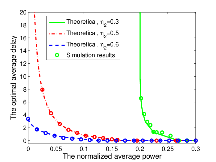
Fig. 3 plots the optimal delay-power tradeoff performance for Case I. It is observed from Fig. 3(a) that the minimum average queueing delay monotonically decreases with the increase of the maximum power consumption $p_{max}$ , which contributes to the growth of the service rate. That is, when more power can be drawn from the RES, the packets will be transmitted more quickly and the queueing delay is reduced. One can see that the minimum average queueing delay decreases from infinity to zero, when $p_{max}$ grows from zero to $\tilde{p}_{0}$ , which is equal to $\frac{\mu_{2}}{Q_{2}+\phi_{1}^{-1}}$ in the case of $\eta_{1}=\eta_{2}$ . Hence, the decreasing rate grows with the increase of the battery capacity $Q_{2}$ . This means that a larger $Q_{2}$ leads to a much smaller queueing delay, since less harvested energy is wasted due to the limitation of the battery capacity. Fig. 3(b) demonstrates the optimal delay-power performance for different energy arrival rates $\eta_{2}$ . When $\eta_{2}\leq\eta_{1}$ , the average delay is infinite at $p_{max}=0$ , since the arrival rate is greater than or equal to the service rate. Therefore, the source should exploit extra energy from the RES to transmit backlogged packets, corresponding to a positive $p_{max}$ . While the source can rely only on the harvested energy to transmit, $i.e.$ , $p_{max}=0$ , when $\eta_{2}>\eta_{1}$ .

Fig. 4 shows the optimal delay-power tradeoff performance of the proposed scheme in Case II with $k_{2}=2,\cdots,6$ . The optimal delay-power curve of the case with $k_{1}=k_{2}=1$ is also plotted for comparison. In this experiment, we set $\eta_{1}=0.5$ , $\eta_{2}=0.1$ and $Q_{2}=5$ . From this figure, one can see that there exists an optimal delay-power tradeoff for each $k_{2}$ . The average queueing delay monotonically decreases with the increase of the maximum allowable power consumption $p_{max}$ from the RES due to the enhanced service rate. For the same reason, a larger $k_{2}$ means a higher amount of energy harvested each time, and leads to a much better delay-power tradeoff. It is also observed the delay-power curves of $k_{2}=5$ and $k_{2}=6$ are almost identical to each other. This owes to the fact that in the case of $k_{2}=6$ , a part of harvest energy is wasted when recharging the battery with capacity $Q_{2}=5$ .

Similarly, we plot the optimal delay-power curves of the proposed scheme for Case III with different $k_{1}$ in Fig. 5. We set $\eta_{1}=0.1,\eta_{2}=0.3$ , and $Q_{2}=5$ . Similar to Case II shown in Fig. 4, a higher $p_{max}$ induces reduced average queueing delay thanks to the enhanced service rate. The only difference between them is the behavior of the minimum average delay $\bar{D}^{*}$ . In Case I with $k_{1}=k_{2}=1$ , the average queueing delay is equal to zero if there exists sufficient energy whether from the battery or the RES, since one newly arriving data packet can always be delivered immediately. In Case III, however, at most one of $k_{1}$ data packets that newly arrive at this slot can be delivered, and the other packets shall wait for the next transmission opportunity. And more packets are queued when the data arrival rate is increased due to the growth of $k_{1}$ or $\eta_{1}$ . As shown in Fig. 5, $\bar{D}^{*}$ increases with the increase of $k_{1}$ .

VII Conclusions

In this paper, we investigated the delay optimal scheduling problem over a communication link. The source node can rely on energy supply either from an energy harvesting battery of finite capacity or from the RES subject to a maximum power consumption from the RES. Using the two-dimensional Markov chain modeling, we formulated an LP problem and studied the structure of the optimal solution. As a result, we obtained the optimal scheduling policy through rigorous derivation and algorithm design.

It is found that the source should schedule packet transmissions according to a critical threshold on the data queue length. Specifically, the source should always wait for the harvested energy when the data queue length is below the optimal threshold $i^{*}$ , and resort to the RES when the data queue length exceeds the threshold $i^{*}$ while no harvested energy can be exploited. The optimal threshold $i^{*}$ is determined by the maximum allowable power from the RES $p_{max}$ . Simulation results confirmed our theoretical analysis. It was shown that there always exists an optimal delay-power tradeoff and its decreasing rate depends on the energy arrival rate and the battery capacity.

In this work, we assume that the Bernoulli data and energy arrival processes generate integral packets probabilistically, and only one data packet is transmitted in each slot. In the future, we will extend the study to the scenario where rate-flexible physical-layer transmissions are scheduled based on the randomly available amount of harvested energy and time-varying wireless channel conditions.

-A Proof of Lemma 2

By applying the stochastic scheduling scheme described in Section II.2, the source shall resort to the RES only when the harvested energy is not available in the current slot. Thus, the state set $\mathcal{Q}_{p}$ (c.f. (8)) is given by $\{(0,0),(1,0),\cdots,(Q_{1},0)\}$ . Recall that the source will draw the reliable energy to transmit with probability $g_{i}$ if new data packets arrive and with probability $f_{i}$ if no data packets arrive, respectively. Hence, the reliable energy consumption at state $(i,0)$ can be expressed as $\omega_{(0,0)}(p)=\mu_{2}g_{0}$ and $\omega_{(i,0)}(p)=\mu_{2}g_{i}+\mu_{1}f_{i}$ $(i>0)$ , respectively. Consequently, the normalized average power consumed from the RES can be obtained as $\bar{P}=\sum_{i=0}^{Q_{1}}\pi_{(i,0)}\omega_{(i,0)}(p)=\sum_{i=0}^{Q_{1}}\pi_{(i,0)}\mu_{2}g_{i}+\sum_{i=1}^{Q_{1}}\pi_{(i,0)}\mu_{1}f_{i}$ . The following result eliminates the dependence of $\bar{P}$ on the transmission parameters and presents a unified expression for all three cases.

1) In Case I, from Fig. 2(c), the local equilibrium equation of the Markov chain can be expressed as

\pi_{(i,0)}\lambda_{1,i}=\pi_{(i+1,0)}\tilde{\mu}_{1,i+1},\,\pi_{(0,j)}\mu_{0}=\pi_{(0,j+1)}\mu_{2},

(24)

for all $i\in\{0,\cdots,Q_{1}-1\}$ and $j\in\{0,\cdots,Q_{2}-2\}$ , and $\pi_{(0,Q_{2}-1)}\mu_{0}=\pi_{(0,Q_{2})}\eta_{1}$ . From (24), we have $\pi_{(0,0)}\lambda_{1,0}=\sum_{i=1}^{Q_{1}}\pi_{(i,0)}(\tilde{\mu}_{1,i}-\lambda_{1,i})$ , where $\pi_{(Q_{1},0)}\lambda_{1,Q_{1}}=0$ is introduced for notational convenience. With $\lambda_{1,i}=\mu_{2}(1-g_{i})$ (c.f. (10)) and $\tilde{\mu}_{1,i}=\mu_{0}+\mu_{1}f_{i}$ (c.f. (11)), the normalized average power consumption from the RES $\bar{P}$ can also be expressed as

\begin{split}\bar{P}=&\pi_{(0,0)}\mu_{2}g_{0}+\sum\nolimits_{i=1}^{Q_{1}}\pi_{(i,0)}(\mu_{2}g_{i}+\mu_{1}f_{i})\\ =&\pi_{(0,0)}(\mu_{2}-\lambda_{1,0})+\sum\nolimits_{i=1}^{Q_{1}}\pi_{(i,0)}(\mu_{2}-\lambda_{1,i}+\tilde{\mu}_{1,i}-\mu_{0})\\ =&\pi_{(0,0)}\mu_{2}+(\mu_{2}-\mu_{0})\sum\nolimits_{i=1}^{Q_{1}}\pi_{(i,0)}.\end{split}

Hence, we get $\xi_{0}=\mu_{2}$ , $\xi_{i}=\mu_{2}-\mu_{0}$ for all $i\in\mathcal{Q}_{1}^{R}$ and $\zeta_{i}=0$ for all $i\in\mathcal{Q}_{1}$ .

2) From Fig. 2(d) for Case II, the local equilibrium equation at state $(0,0)$ can be expressed as $\pi_{(1,0)}\mu_{1,1}-\pi_{(0,0)}\lambda_{1,0}=\eta_{2}\pi_{(0,0)}-\mu_{2}\pi_{(0,1)}-\mu_{1}\pi_{(1,1)}$ . Following a similar procedure, the local equilibrium equation at state $(i,0)$ ( $i\geq 1$ ) is thus

\begin{split}&\pi_{(i+1,0)}\mu_{1,i+1}-\pi_{(i,0)}\lambda_{1,i}=\pi_{(i,0)}\mu_{1,i}-\pi_{(i-1,0)}\lambda_{1,i-1}\\ &+(\mu_{0}+\mu_{3})\pi_{(i,0)}-\mu_{2}\pi_{(i,1)}-\mu_{1}\pi_{(i+1,1)}\\ =&\eta_{2}\sum\nolimits_{m=0}^{i}\pi_{(m,0)}-\mu_{2}\sum\nolimits_{m=0}^{i}\pi_{(m,1)}-\mu_{1}\sum\nolimits_{m=1}^{i+1}\pi_{(m,1)},\end{split}

where the second equality is obtained through recursion of $(\pi_{(i,0)}\mu_{1,i}-\pi_{(i-1,0)}\lambda_{1,i-1})$ . Hence, we can compute the normalized average power consumption as

\begin{split}\bar{P}&=\sum\nolimits_{i=0}^{Q_{1}}\pi_{(i,0)}(\mu_{2}-\lambda_{1,i})+\sum\nolimits_{i=1}^{Q_{1}}\pi_{(i,0)}\mu_{1}f_{i}\\ =&\mu_{2}\sum\nolimits_{i=0}^{Q_{1}}\pi_{(i,0)}+\sum\nolimits_{i=1}^{Q_{1}}\left(\pi_{(i,0)}\mu_{1,i}-\pi_{(i-1,0)}\lambda_{1,i-1}\right)\\ =&\sum\nolimits_{i=0}^{Q_{1}}\pi_{(i,0)}(\mu_{2}+\eta_{2}(Q_{1}-i))\\ &-\mu_{2}Q_{1}\pi_{(0,1)}-\sum\nolimits_{i=1}^{Q_{1}}(\bar{\eta}_{2}(Q_{1}-i)+\mu_{1})\pi_{(i,1)},\end{split}

where the second equality is due to the fact that $\mu_{1,i}=\mu_{1}f_{i}$ , and the third equality is obtained through the summation of $\pi_{(i,0)}\mu_{1,i}-\pi_{(i-1,0)}\lambda_{1,i-1}$ over all $i>0$ . In this way, we get $\xi_{i}=\mu_{2}+\eta_{2}(Q_{1}-i)$ for all $i\in\mathcal{Q}_{1}$ , $\zeta_{0}=\mu_{2}Q_{1}$ , and $\zeta_{i}=\bar{\eta}_{2}(Q_{1}-i)+\mu_{1}$ for all $i\in\mathcal{Q}_{1}^{R}$ .

3) In Case III, the corresponding Markov chain is depicted in Fig. 2(e). When $i<k_{1}-1$ , the local balance equation at state $(i,0)$ is given by

\begin{split}&\tilde{\mu}_{1,i+1}\pi_{(i+1,0)}=\pi_{(i,0)}\tilde{\mu}_{1,i}+\pi_{(i,0)}(\lambda_{1,i}+\tilde{\lambda}_{1,i})-\mu_{1}\pi_{(i+1,1)}\\ =&\pi_{(0,0)}\mu_{0}+\sum\nolimits_{m=0}^{i}\pi_{(m,0)}\eta_{1}-\sum\nolimits_{m=1}^{i+1}\mu_{1}\pi_{(m,1)},\end{split}

where $\lambda_{1,i}+\tilde{\lambda}_{1,i}=\eta_{1}$ (c.f. (12)) is applied. When $i\geq k_{1}-1$ , the local balance equation at state $(i,0)$ can be expressed as

\begin{split}&\pi_{(i-k_{1}+1,0)}\tilde{\lambda}_{1,i-k_{1}+1}+\tilde{\mu}_{1,i+1}\pi_{(i+1,0)}\\ =&\pi_{(i,0)}\tilde{\mu}_{1,i}-\lambda_{1,i-k_{1}}\pi_{(i-k_{1},0)}+\pi_{(i,0)}(\lambda_{1,i}+\tilde{\lambda}_{1,i})\\ &-\mu_{2}\pi_{(i-k_{1}+1,1)}-\mu_{1}\pi_{(i+1,1)}=\eta_{1}\sum_{m=i-k_{1}+1}^{i}\pi_{(m,0)}\\ &+\pi_{(0,0)}\mu_{0}-\mu_{1}\sum\nolimits_{m=1}^{i+1}\pi_{(m,1)}-\mu_{2}\sum\nolimits_{m=0}^{i-k_{1}+1}\pi_{(m,1)}.\end{split}

Then, we can compute the normalized average power consumption as

\begin{split}\bar{P}=&\sum\nolimits_{i=0}^{Q_{1}}\pi_{(i,0)}\mu_{2}g_{i}+\sum\nolimits_{i=1}^{Q_{1}}\pi_{(i,0)}\mu_{1}f_{i}\\ =&\sum\nolimits_{i=k_{1}-1}^{Q_{1}-1}(\pi_{(i-k_{1}+1,0)}\tilde{\lambda}_{1,i-k_{1}+1}+\tilde{\mu}_{1,i+1}\pi_{(i+1,0)})\\ &+\sum\nolimits_{i=0}^{k_{1}-2}\tilde{\mu}_{1,i+1}\pi_{(i+1,0)}-\mu_{3}\pi_{(0,0)}-\eta_{2}\sum\nolimits_{i=1}^{Q_{1}}\pi_{(i,0)}\\ =&\sum\nolimits_{i=0}^{Q_{1}}\xi_{i}\pi_{(i,0)}-\sum\nolimits_{i=0}^{Q_{1}}\zeta_{i}\pi_{(i,1)}.\end{split}

where the second equality is due to the fact that $\tilde{\lambda}_{1,i}=\mu_{3}+\mu_{2}g_{i}$ (c.f. (12)) and $\tilde{\mu}_{1,i}=\mu_{0}+\mu_{1}f_{i}$ (c.f. (11)), the last equality is obtained via the summation of $\pi_{(i-k_{1}+1,0)}\tilde{\lambda}_{1,i-k_{1}+1}+\tilde{\mu}_{1,i+1}\pi_{(i+1,0)}$ and $\tilde{\mu}_{1,i+1}\pi_{(i+1,0)}$ over $i\geq k_{1}-1$ and $i<k_{1}-1$ , respectively. As a result, we can compute the coefficients $\xi_{i}$ and $\zeta_{i}$ as listed in Table I.

-B Proof of Lemma 3

We will prove that for each $i$ , the probability $\pi_{i}$ satisfies the inequality (15) for Cases I, II and III, respectively.

1) In Case I, we have $\lambda_{1,i}=\mu_{2}(1-g_{i})$ and $\tilde{\mu}_{1,i}=\mu_{0}+\mu_{1}f_{i}$ , which satisfy $0\leq\lambda_{1,i}\leq\mu_{2},\,\mu_{0}\leq\tilde{\mu}_{1,i}\leq\mu_{0}+\mu_{1}=\bar{\eta}_{1}$ , since $0\leq g_{i}\leq 1$ and $0\leq f_{i}\leq 1$ . From the local equilibrium equation (24), we have $0\leq\pi_{i}=\pi_{(i,0)}\leq\phi\pi_{(i-1,0)}$ , since $0\leq\frac{\pi_{(i,0)}}{\pi_{(i-1,0)}}=\frac{\lambda_{1,i-1}}{\tilde{\mu}_{1,i}}\leq\frac{\mu_{2}}{\mu_{0}}=\phi$ . In this case, we have $\Theta_{u}(i,\tilde{\bm{\pi}}_{i})=\phi\pi_{(i-1,0)}$ when $g_{i-1}=0$ and $f_{i}=0$ , and $\Theta_{l}(i,\tilde{\bm{\pi}}_{i-1})=0$ when $g_{i-1}=1$ .

2) From Fig. 2(d) in Case II, the local balance equation $\pi_{(i-1,0)}\lambda_{1,i-1}=\pi_{(i,0)}(\mu_{1,i}+\mu_{0})+(\mu_{0}+\mu_{1})\sum_{j=1}^{Q_{2}-1}\pi_{(i,j)}+\bar{\eta}_{1}\pi_{(i,Q_{2})}$ holds for all $i>0$ , thus leading to $\pi_{(i-1,0)}\lambda_{1,i-1}=\pi_{(i,0)}(\mu_{1,i}+\mu_{0})+\bar{\eta}_{1}\sum\nolimits_{j=1}^{Q_{2}}\pi_{(i,j)}$ because of $\mu_{0}+\mu_{1}=\bar{\eta}_{1}$ . Hence, we have $\bar{\eta}_{1}\pi_{i}=\bar{\eta}_{1}\sum\nolimits_{j=0}^{Q_{2}}\pi_{(i,j)}=\pi_{(i-1,0)}\lambda_{1,i-1}-\pi_{(i,0)}(\mu_{1,i}+\mu_{0})+\bar{\eta}_{1}\pi_{(i,0)}$ . Since $0\leq g_{i}\leq 1$ and $0\leq f_{i}\leq 1$ , we get $0\leq\lambda_{1,i}=\mu_{2}(1-g_{i})\leq\mu_{2}$ and $\mu_{0}\leq\mu_{1,i}+\mu_{0}=\mu_{1}f_{i}+\mu_{0}\leq\bar{\eta}_{1}$ . With the varying parameter $\{\lambda_{1,i}\}$ and $\{\mu_{1,i}\}$ , we further have $0\leq\pi_{i}\leq\Theta_{u}(i,\tilde{\bm{\pi}}_{i})$ , where $\pi_{i}=\Theta_{u}(i,\tilde{\bm{\pi}}_{i})=\tau\bar{\eta}_{2}\pi_{(i-1,0)}+\pi_{(i,0)}\bar{\eta}_{2}$ when $\lambda_{1,i-1}=\mu_{2}$ and $\mu_{1,i}+\mu_{0}=\mu_{0}$ ( $g_{i-1}=f_{i}=0$ ), and $\pi_{i}=\Theta_{l}(i,\tilde{\bm{\pi}}_{i-1})=0$ when $\lambda_{1,i-1}=0$ and $\mu_{1,i}+\mu_{0}=\bar{\eta}_{1}$ ( $g_{i-1}=f_{i}=1$ ), respectively.

3) In Case III, from Fig. 2(e), the local equilibrium equation between states $(i-1,j)$ and $(i,j)$ $(j\in\mathcal{Q}_{2})$ can be expressed as $\sum_{m=0}^{i-1}\pi_{(m,0)}(\lambda_{1,m}+\tilde{\lambda}_{1,m})+(\mu_{2}+\mu_{3})\sum_{m=0}^{i-1}\sum_{j=1}^{Q_{2}-1}\pi_{(m,j)}+\eta_{1}\sum_{m=0}^{i-1}\pi_{(m,Q_{2})}=\pi_{(i,0)}\tilde{\mu}_{1,i}+(\mu_{0}+\mu_{1})\sum_{j=1}^{Q_{2}-1}\pi_{(i,j)}+\bar{\eta}_{1}\pi_{(i,Q_{2})}$ for all $i<k_{1}$ . With $\lambda_{1,i-1}+\tilde{\lambda}_{1,i-1}=\mu_{2}+\mu_{3}=\eta_{1}$ and $\mu_{0}+\mu_{1}=\bar{\eta}_{1}$ , it can be rewritten as $\eta_{1}\sum_{m=0}^{i-1}\pi_{m}=\pi_{(i,0)}\tilde{\mu}_{1,i}+\bar{\eta}_{1}\sum_{j=1}^{Q_{2}}\pi_{(i,j)}$ .

Since $\mu_{0}\leq\tilde{\mu}_{1,i}=\mu_{0}+\mu_{1}f_{i}\leq\bar{\eta}_{1}$ , we get $\Theta_{l}(i,\tilde{\bm{\pi}}_{i-1})\leq\bar{\eta}_{1}\sum_{j=0}^{Q_{2}}\pi_{(i,j)}\leq\Theta_{u}(i,\tilde{\bm{\pi}}_{i})$ . Thus, $\pi_{i}=\Theta_{u}(i,\tilde{\bm{\pi}}_{i})=\frac{\mu_{1}}{\bar{\eta}_{1}}\pi_{(i,0)}+\frac{\eta_{1}}{\bar{\eta}_{1}}\sum_{m=0}^{i-1}\pi_{m}$ when $\tilde{\mu}_{1,i}=\mu_{0}$ ( $f_{i}=0$ ), and $\pi_{i}=\Theta_{l}(i,\tilde{\bm{\pi}}_{i-1})=\frac{\eta_{1}}{\bar{\eta}_{1}}\sum_{m=0}^{i-1}\pi_{m}$ when $\tilde{\mu}_{1,i}=\bar{\eta}_{1}$ ( $f_{i}=0$ ), respectively.

Similarly, when $i\geq k_{1}$ , the corresponding local equilibrium equation between states $(i-1,j)$ and $(i,j)$ is given by $\eta_{1}\sum_{m=i-k_{1}+1}^{i-1}\pi_{m}=\pi_{(i,0)}\tilde{\mu}_{1,i}-\pi_{(i-k_{1},0)}\lambda_{1,i-k_{1}}+\bar{\eta}_{1}\sum_{j=1}^{Q_{2}}\pi_{(i,j)}$ . Since $0\leq\lambda_{1,i}=\mu_{2}(1-g_{i})\leq\mu_{2}$ and $\mu_{0}\leq\tilde{\mu}_{1,i}=\mu_{0}+\mu_{1}f_{i}\leq\bar{\eta}_{1}$ , we get $\eta_{1}\sum_{m=i-k_{1}+1}^{i-1}\pi_{m}\leq\bar{\eta}_{1}\sum_{j=0}^{Q_{2}}\pi_{(i,j)}\leq\mu_{2}\pi_{(i-k_{1},0)}+\mu_{1}\pi_{(i,0)}+\eta_{1}\sum_{m=i-k_{1}+1}^{i-1}\pi_{m}$ . Thus, $\pi_{i}=\Theta_{u}(i,\tilde{\bm{\pi}}_{i})=\frac{\mu_{2}}{\bar{\eta}_{1}}\pi_{(i-k_{1},0)}+\frac{\mu_{1}}{\bar{\eta}_{1}}\pi_{(i,0)}+\frac{\eta_{1}}{\bar{\eta}_{1}}\sum_{m=i-k_{1}+1}^{i-1}\pi_{m}$ when $\lambda_{1,i-k_{1}}=\mu_{2}$ and $\tilde{\mu}_{1,i}=\mu_{0}$ ( $g_{i-k_{1}}=0,f_{i}=0$ ), $\pi_{i}=\Theta_{l}(i,\tilde{\bm{\pi}}_{i-1})=\frac{\eta_{1}}{\bar{\eta}_{1}}\sum_{m=0}^{i-1}\pi_{m}$ when $\lambda_{1,i-k_{1}}=0$ and $\tilde{\mu}_{1,i}=\bar{\eta}_{1}$ ( $g_{i-k_{1}}=1,f_{i}=1$ ), respectively.

Combining the above two cases: $i<k_{1}$ and $i\geq k_{1}$ , we get $\Theta_{u}(i,\tilde{\bm{\pi}}_{i})$ and $\Theta_{l}(i,\tilde{\bm{\pi}}_{i-1})$ as listed in Table II.

-C Proof of Theorem 4

Subject to the constraint (13.b), we have $\bar{D}=\frac{1}{k_{1}\eta_{1}}\sum\nolimits_{i=1}^{Q_{1}}i\pi_{i}\geq\frac{1}{k_{1}\eta_{1}}\sum\nolimits_{i=1}^{Q_{1}}i\Theta_{l}(i,\tilde{\bm{\pi}}_{i-1})$ . This means that the average queuing delay $\bar{D}$ , as a weighted summation of $\pi_{i}$ , can be minimized, if each $\pi_{i}$ chooses its lower bound $\Theta_{l}(i,\tilde{\bm{\pi}}_{i-1})$ for all $i\geq 1$ . From Lemma 3, this happens when all the transmission parameters satisfy $g_{i-k_{1}}=f_{i}=1$ for all $i>0$ . This corresponds to the scheduling policy based on the optimal threshold $i^{*}=0$ and the corresponding average power consumption from the RES is $\tilde{p}_{0}$ . Hence, when $p_{max}\geq\tilde{p}_{0}$ , the minimum average queueing delay $\bar{D}^{*}$ is obtained if $\pi_{i}^{*}=\Theta_{l}(i,\tilde{\bm{\pi}}_{i-1}^{*})$ or $\bm{\pi}^{*}\bm{a}_{i}^{l}=0$ for all $i=1,\cdots,Q_{1}$ , and the optimal threshold $i^{*}$ is zero. When $k_{1}\eta_{1}-k_{2}\eta_{2}<p_{max}<\tilde{p}_{0}$ , $g_{i-k_{1}}=f_{i}=1$ does not hold for all $i>0$ and hence there must exist $i^{*}>0$ .

-D Proof of Theorem 5

Subject to the constraint $\sum_{i=0}^{Q_{1}}\pi_{i}=1$ , The average queueing delay $\bar{D}=\frac{1}{k_{1}\eta_{1}}\sum_{i=1}^{Q_{1}}i\pi_{i}$ can be minimized, if each $\pi_{i}$ chooses its lower bound $\Theta_{l}(i,\tilde{\bm{\pi}}_{i-1})$ for all $i\geq 1$ , corresponding to the case when $p_{max}\geq\tilde{p}_{0}$ shown in the proof of Theorem 4. Here, we focus on studying the optimal solution in the case when $k_{1}\eta_{1}-k_{2}\eta_{2}<p_{max}<\tilde{p}_{0}$ . In this case, $\bar{P}=\sum_{i=0}^{Q_{1}}\xi_{i}\pi_{(i,0)}^{*}-\sum_{i=0}^{Q_{1}}\zeta_{i}\cdot\pi_{(i,1)}^{*}=p_{max}$ is straightforward. This lies in the fact that the data queue length becomes smaller when more reliable energy can be exploited to transmit backlogged data packets.

In the sequel, we will show that when $k_{1}\eta_{1}-k_{2}\eta_{2}<p_{max}<\tilde{p}_{0}$ , the average queueing delay can also be minimized, if the optimal solution $\bm{\pi}^{*}$ satisfies (16) ( $\pi_{0}$ , $\pi_{1}$ , $\cdots$ , $\pi_{i^{*}-1}$ are assigned to their upper bounds and $\pi_{i^{*}+1},\cdots,\pi_{Q_{1}}$ are assigned to their lower bounds) for Cases I, II, and III, respectively.

-D1 Case I

From Lemma 1, we only need to consider the steady-state probabilities $\pi_{(i,0)}$ and $\pi_{(0,j)}$ for all $i\in\mathcal{Q}_{1}$ and $j\in\mathcal{Q}_{2}$ . The constraint $\sum_{j=0}^{Q_{2}}\pi_{(i,j)}\geq\Theta_{l}(i,\tilde{\bm{\pi}}_{i-1})=0$ naturally holds since $\pi_{(i,j)}\geq 0$ , and hence we do not consider the corresponding constraints $\sum_{j=0}^{Q_{2}}\pi_{(i,j)}\geq 0$ ( $i>0$ ).

From the Markov chain in Fig. 2(c), the optimal solution $\pi_{(0,j)}^{*}$ satisfies $\mu_{2}\pi_{(0,j)}^{*}=\mu_{0}\pi_{(0,j-1)}^{*}$ for $j=1,\cdots,Q_{2}-1$ and $\eta_{1}\pi_{(0,Q_{2})}^{*}=\mu_{0}\pi_{(0,Q_{2}-1)}^{*}$ for $j=Q_{2}$ . Hence, the probability that the data queue length is zero is obtained as $\pi_{0}^{*}=\pi_{(0,0)}^{*}+\pi_{(0,0)}^{*}\sum\limits_{j=1}^{Q_{2}-1}\phi^{-j}+\frac{\pi_{(0,0)}^{*}}{\phi^{Q_{2}-1}\phi_{1}}=\alpha\pi_{(0,0)}^{*}$ , where $\alpha=\sum_{i=0}^{Q_{2}-1}\phi^{-i}+\phi^{-(Q_{2}-1)}\phi_{1}^{-1}$ . Thus, we have $\sum_{i=1}^{Q_{1}}\pi_{(i,0)}^{*}=1-\pi_{0}^{*}=1-\alpha\pi_{(0,0)}^{*}$ . And the normalized average power consumption from the RES is $\bar{P}=\mu_{2}\pi_{(0,0)}^{*}+(\mu_{2}-\mu_{0})\sum_{i=1}^{Q_{1}}\pi_{(i,0)}^{*}=\mu_{2}\pi_{(0,0)}^{*}+(\mu_{2}-\mu_{0})(1-\alpha\pi_{(0,0)}^{*})$ , from which we obtain $\pi_{(0,0)}^{*}=\frac{p_{max}-(\mu_{2}-\mu_{0})}{\mu_{2}-\alpha(\mu_{2}-\mu_{0})}$ . Hence, $\pi_{(0,0)}^{*}$ depends only on $p_{max}$ . As shown in the proof of Theorem 4, when $p_{max}\geq\tilde{p}_{0}$ , we have $\pi_{0}^{*}=\alpha\pi_{(0,0)}^{*}=1$ and thus $\pi_{(0,0)}^{*}=\frac{1}{\alpha}$ . When $p_{max}<\tilde{p}_{0}$ , there must exist $\pi_{(0,0)}^{*}<\frac{1}{\alpha}$ and $\sum_{i=1}^{Q_{1}}\pi_{(i,0)}^{*}>0$ .

By contradiction, we will show that the optimal solution $\pi_{(i,0)}^{*}$ satisfies (16): $\pi_{(i,0)}^{*}=\phi\pi_{(i-1,0)}^{*}$ for $i<i^{*}$ , $0<\pi_{(i,0)}^{*}<\phi\pi_{(i-1,0)}^{*}$ for $i=i^{*}$ , and $\pi_{(i,0)}^{*}=0$ for $i>i^{*}$ , since it leads to the minimum average queueing delay. Suppose that there exists another set of steady-state probabilities $\pi_{(i,0)}$ : $\pi_{(i,0)}=\pi_{(i,0)}^{*}=\pi_{(0,0)}^{*}\phi^{i}$ for $0\leq i<m$ , and $0<\pi_{(m,0)}<\phi\pi_{(m-1,0)}$ for $m\leq i\leq i_{1}$ . Subject to $\pi_{0}+\sum_{i=1}^{i_{1}}\pi_{(i,0)}=\pi_{0}^{*}+\sum_{i=1}^{i^{*}}\pi_{(i,0)}^{*}=1$ , there must exist $\pi_{(i,0)}<\pi_{(i,0)}^{*}$ for $m\leq i<i^{*}$ and $\sum_{i=i^{*}}^{i_{1}}\pi_{(i,0)}-\pi_{(i^{*},0)}^{*}=\sum_{i=m}^{i^{*}-1}(\pi_{(i,0)}^{*}-\pi_{(i,0)})$ with $i_{1}\geq i^{*}$ . Thus, we have $i^{*}(\sum_{i=i^{*}}^{i_{1}}\pi_{(i,0)}-\pi_{(i^{*},0)}^{*})=i^{*}\sum_{i=m}^{i^{*}-1}(\pi_{(i,0)}^{*}-\pi_{(i,0)})$ . Hence, the corresponding average queueing delay $\bar{D}=\frac{1}{\eta_{1}}\sum_{i=1}^{i_{1}}i\cdot\pi_{(i,0)}$ satisfies

\begin{array}[]{rl}&\bar{D}=\frac{1}{\eta_{1}}\sum_{i=1}^{i^{*}}i\cdot\pi_{(i,0)}^{*}-\frac{1}{\eta_{1}}\sum_{i=1}^{i^{*}-1}i\cdot(\pi_{(i,0)}^{*}-\pi_{(i,0)})\\ &+\frac{1}{\eta_{1}}(\sum_{i=i^{*}}^{i_{1}-1}i\pi_{(i,0)}-i^{*}\pi_{(i^{*},0)}^{*})>\bar{D}^{*}.\end{array}

As a result, we can obtain the minimum average queueing delay when the optimal solution $\bm{\pi}^{*}$ satisfies (16).

-D2 Case II

Similar to Case I, we have $\Theta_{l}(i,\tilde{\bm{\pi}}_{i-1})=0$ , as listed in Table II. From the corresponding Markov chain shown in Fig. 2(d), we have $\pi_{i}=\Theta_{l}(i,\tilde{\bm{\pi}}_{i-1})=0$ and $\pi_{(i,j)}=0$ for all $i>m$ , if $\pi_{m}=\Theta_{l}(m,\tilde{\bm{\pi}}_{m-1})$ holds. We first show that $\pi_{i}=\Theta_{l}(i,\tilde{\bm{\pi}}_{i-1})$ does not hold for $i\leq i^{*}$ . If the solution $\bm{\pi}$ satisfies $0<\pi_{i}\leq\Theta_{u}(i,\tilde{\bm{\pi}}_{i})$ for $1<i<i_{1}$ and $\pi_{i_{1}}=\Theta_{l}(i_{1},\tilde{\bm{\pi}}_{i_{1}-1})$ for some $i_{1}\leq i^{*}$ , the corresponding power consumption from the RES $\bar{P}$ will be larger than $p_{max}$ , since it satisfies $\bar{P}\geq\tilde{p}_{i_{1}-1}\geq\tilde{p}_{i^{*}-1}>p_{max}\geq\tilde{p}_{i^{*}}$ ( $\tilde{p}_{m}$ decreases with the threshold $m$ ). This violates the constraint (13.a). Hence, the solution $\bm{\pi}^{*}$ should satisfy $0<\pi_{i}^{*}\leq\Theta_{u}(i,\tilde{\bm{\pi}}_{i}^{*})$ for $0<i\leq i_{1}$ , and $\pi_{i}^{*}=\Theta_{l}(i,\tilde{\bm{\pi}}_{i-1}^{*})=0$ for $i\geq i_{1}>i^{*}$ , respectively. Then, we show that among all the candidate solutions, the solution $\bm{\pi}^{*}$ satisfying (16) leads to the minimum queueing delay. According to the condition, we have $0<\pi_{i}\leq\tau\bar{\eta}_{2}\pi_{(i-1,0)}+\pi_{(i,0)}\bar{\eta}_{2}$ for $0<i\leq i_{1}$ . In this case, the solution $\bm{\pi}^{*}$ satisfies $\pi_{i}^{*}=\sum_{j=0}^{Q_{2}}\pi_{(i,j)}^{*}=\tau\bar{\eta}_{2}\pi_{(i-1,0)}^{*}+\bar{\eta}_{2}\pi_{(i,0)}^{*}$ for $0<i<i^{*}$ and the minimum average queueing delay is $\bar{D}^{*}=\sum_{i=1}^{i^{*}}i\pi_{i}^{*}$ . Suppose that there is a solution $\bm{\pi}$ that satisfies $\pi_{i}=\tau\bar{\eta}_{2}\pi_{(i-1,0)}+\bar{\eta}_{2}\pi_{(i,0)}$ for $0<i<m$ , $0<\pi_{m}<\tau\bar{\eta}_{2}\pi_{(m-1,0)}+\bar{\eta}_{2}\pi_{(m,0)}$ for some $m\leq i^{*}-1$ , and $0<\pi_{i}\leq\tau\bar{\eta}_{2}\pi_{(i-1,0)}+\bar{\eta}_{2}\pi_{(i,0)}$ for $m<i\leq i_{1}$ . Subject to $\sum_{i=0}^{i*}\pi_{i}^{*}=\sum_{i=0}^{i_{1}}\pi_{i}=1$ , the average queueing delay $\bar{D}=\frac{1}{\eta_{1}}\sum_{i=1}^{i_{1}}i\cdot\pi_{i}$ satisfies

\begin{array}[]{l}\bar{D}=\frac{1}{\eta_{1}}\sum_{i=1}^{i^{*}}i\cdot\pi_{i}^{*}+\frac{1}{\eta_{1}}(\sum_{i=1}^{i^{*}-1}i\cdot(\pi_{i}-\pi_{i}^{*})\\ +(\sum_{i=i^{*}}^{i_{1}}i\pi_{i}-i^{*}\pi_{i^{*}}^{*}))>\bar{D}^{*}+\frac{1}{\eta_{1}}\sum_{i=0}^{i^{*}-1}(i^{*}-i)(\pi_{i}^{*}-\pi_{i})\\ =\bar{D}^{*}+\frac{1}{\eta_{1}}\sum_{i=0}^{i^{*}-1}(i^{*}-i)\bar{\eta}_{2}(\pi_{(i,0)}^{*}-\pi_{(i,0)})\\ \quad+\frac{1}{\eta_{1}}\sum_{i=0}^{i^{*}-2}(i^{*}-i-1)\tau\bar{\eta}_{2}(\pi_{(i,0)}^{*}-\pi_{(i,0)})\geq\bar{D}^{*}\end{array}

where the first inequality holds since $\sum_{i=i^{*}}^{i_{1}}i\pi_{i}-i^{*}\pi_{i^{*}}^{*}=\sum_{i=0}^{i^{*}-1}i^{*}(\pi^{*}-\pi_{i})+\sum_{i=i^{*}+1}^{i_{1}}(i-i^{*})\pi_{i}>\sum_{i=0}^{i^{*}-1}i^{*}(\pi^{*}-\pi_{i})$ , the last two inequalities hold since we obtain $\pi_{0}>\bar{\eta}_{2}\pi_{(0,0)}$ and $\sum_{i=0}^{i^{*}-1}\pi_{(i,0)}^{*}\geq\sum_{i=0}^{i^{*}-1}\pi_{(i,0)}$ based on the property of the Markov chain. Hence, the optimal solution $\bm{\pi}^{*}$ should satisfy (16) to minimize the average queueing delay.

-D3 Case III

In this case, we have $\Theta_{l}(i,\tilde{\bm{\pi}}_{i-1})=\tau\sum_{m=[i-k_{1}+1]^{+}}^{i-1}\pi_{m}>0$ . Note that $Q_{1}$ should be sufficiently large to avoid buffer overflow. To decrease the average queueing delay $\bar{D}=\frac{1}{k_{1}\eta_{1}}\sum_{i=1}^{Q_{1}}i\pi_{i}$ , $\pi_{i}$ with large index should be assigned its lower bound $\tau\sum_{m=[i-k_{1}+1]^{+}}^{i-1}\pi_{m}$ . In this sense, there exists an integer $i_{1}$ that satisfies $\pi_{i}=\tau\sum_{m=[i-k_{1}+1]^{+}}^{i-1}\pi_{m}$ for all $i\geq i_{1}$ . For the same reason as stated in Case II, $i_{1}>i^{*}$ should be satisfied to meet the power consumption (from the RES) constraint $\bar{P}\leq p_{max}$ .

In the same way, we will compare the delay performances between the optimal solution $\bm{\pi}^{*}$ satisfying (16) and a candidate solution $\bm{\pi}$ . Suppose that $\bm{\pi}$ satisfies $\pi_{i}=\Theta_{u}(i,\tilde{\bm{\pi}}_{i})$ for $0<i<m$ , $\Theta_{l}(i,\tilde{\bm{\pi}}_{i-1})<\pi_{m}<\Theta_{u}(i,\tilde{\bm{\pi}}_{i})$ for some $m\leq i^{*}-1$ , and $0<\pi_{i}\leq\Theta_{u}(i,\tilde{\bm{\pi}}_{i})$ for $m<i\leq i_{1}$ . We notice that $\{\pi_{i}^{*}=\tau\sum_{m=[i-k_{1}+1]^{+}}^{i-1}\pi_{m}^{*}\}$ ( $i>i^{*}$ ) is a decreasing sequence (otherwise the data queue will be unstable). So does the sequence $\{\pi_{i}\}$ ( $i>i_{1}$ ). And $\pi_{i}^{*}=\Theta_{u}(i,\tilde{\bm{\pi}}_{i}^{*})$ increases with the growth of $i$ for $0\leq i\leq i^{*}$ . Then, subject to the constraint $\sum_{i=0}^{Q_{1}}\pi_{i}^{*}=\sum_{i=0}^{Q_{1}}\pi_{i}=1$ , we have $\pi_{i}^{*}\geq\pi_{i}$ for $0\leq i\leq i^{*}$ and $\pi_{i}^{*}\leq\pi_{i}$ for $i^{*}<i\leq Q_{1}$ , and $\sum_{i=0}^{i^{*}}(\pi_{i}^{*}-\pi_{i})=\sum_{i=i^{*}+1}^{Q_{1}}(\pi_{i}-\pi_{i}^{*})$ . As a result, the average queueing delay $\bar{D}$ satisfies

\begin{array}[]{l}\bar{D}=\frac{1}{k_{1}\eta_{1}}\sum\limits_{i=1}^{Q_{1}}i\pi_{i}^{*}+\frac{1}{k_{1}\eta_{1}}(\sum\limits_{i=1}^{i^{*}}i(\pi_{i}-\pi_{i}^{*})+\sum\limits_{i=i^{*}+1}^{Q_{1}}i(\pi_{i}-\pi_{i}^{*}))\\ >\bar{D}^{*}+\frac{1}{k_{1}\eta_{1}}(-\sum\limits_{i=1}^{i^{*}}i^{*}(\pi_{i}-\pi_{i}^{*})+\sum\limits_{i=i^{*}+1}^{Q_{1}}i(\pi_{i}-\pi_{i}^{*}))>\bar{D}^{*}.\end{array}

In this way, we show that the optimal solution $\bm{\pi}^{*}$ should satisfy (16) in Case III.

Note that the optimal solution $\bm{\pi}^{*}$ corresponds to the threshold based scheduling policy. Naturally, a larger threshold $m$ leads to a larger queueing delay. Meanwhile, a lower power $\tilde{p}_{m}$ is consumed from the RES. The optimal threshold can be obtained by comparing the maximum allowable power consumption $p_{max}$ with the power thresholds $\{\tilde{p}_{m}\}$ as: $i^{*}=\arg\min_{\tilde{p}_{m}\leq p_{max}}m$ .

-E Proof of Corollary 7

From Theorem 5 and Lemma 3, when $p_{max}\geq\tilde{p}_{0}$ , $\pi_{i}^{*}=\pi_{(i,0)}^{*}=0$ for all $i>0$ . Then, by substituting (18) into the equation $\pi_{(0,0)}^{*}+\sum_{j=1}^{Q_{2}}\pi_{(0,j)}^{*}=1$ , we obtain $\pi_{(0,0)}^{*}=\frac{1}{\alpha}$ . Accordingly, the power threshold $\tilde{p}_{0}=\mu_{2}\pi_{(0,0)}^{*}=\mu_{2}\alpha^{-1}$ because of $g_{0}=1$ . Then, we discuss the optimal solution for the case when $\eta_{1}-\eta_{2}<p_{max}<\tilde{p}_{0}$ . From Theorem 5 and its proof, we know that there exists an optimal threshold $i^{*}>0$ so that $\pi_{(i,0)}^{*}=\phi\pi_{(i-1,0)}^{*}=\pi_{(0,0)}^{*}\phi^{i}$ for $i<i^{*}$ and $\pi_{(i,0)}^{*}=0$ for $i>i^{*}$ , where $\pi_{(0,0)}^{*}=\frac{p_{max}-(\mu_{2}-\mu_{0})}{\mu_{2}-\alpha(\mu_{2}-\mu_{0})}$ . Since $\pi_{0}^{*}=\alpha\pi_{(0,0)}^{*}$ and thus $\sum_{i=1}^{i^{*}}\pi_{(i,0)}^{*}=1-\alpha\pi_{(0,0)}^{*}$ , we obtain $\pi_{(i^{*},0)}^{*}=1-\alpha\pi_{(0,0)}^{*}-\sum_{i=1}^{i^{*}-1}\pi_{(i,0)}^{*}=1-\pi_{(0,0)}^{*}(\alpha+\sum_{i=1}^{i^{*}-1}\phi^{i})$ . From the property of the optimal solution $\pi_{(i,0)}^{*}$ , the optimal threshold $i^{*}$ can be evaluated as $i^{*}=\Omega_{\phi}(\pi_{(0,0)}^{*},1-\alpha\pi_{(0,0)}^{*})$ , which is the integer that satisfies $\pi_{(0,0)}^{*}\sum_{m=1}^{i^{*}-1}\phi^{m}\leq 1-\alpha\pi_{(0,0)}^{*}<\pi_{(0,0)}^{*}\sum_{m=1}^{i^{*}}\phi^{m}$ .

-F Proof of Corollary 8

From Theorem 5 and its proof, the optimal threshold is $i^{*}=0$ when $p_{max}\geq\tilde{p}_{0}$ and hence the optimal solution $\bm{\pi}^{*}$ can be obtained by solving $(1+Q_{1})(1+Q_{2})$ independent linear equations: $\bm{\pi}\bm{a}_{i}^{u}=0$ $(\forall i>0)$ , $\bm{\pi}\tilde{\bm{P}}_{s}=\bm{0}$ , and $\bm{\pi}\bm{e}=1$ . In this case, we get $\bm{\pi}^{*}=\bm{\pi}_{0}^{{}^{\prime}}$ according to (22). When $\tilde{p}_{i^{*}}\leq p_{max}<\tilde{p}_{i^{*}-1}$ , the optimal solution $\bm{\pi}^{*}$ satisfies $\bm{\pi}^{*}\bm{a}_{0}=p_{max}$ , $\bm{\pi}^{*}\bm{a}_{i}^{u}=0\,(i=1,\cdots,i^{*}-1)$ , $\bm{\pi}^{*}\bm{a}_{i}^{l}=0\,(i=i^{*}+1,\cdots,Q_{1})$ , $\bm{\pi}\tilde{\bm{P}}_{s}=\bm{0}$ , and $\bm{\pi}\bm{e}=1$ . Hence, we can obtain $\bm{\pi}^{*}=\bm{b}\bm{A}^{-1}$ by solving $(1+Q_{1})(1+Q_{2})$ linear equations.

-G Proof of Corollary 9

We will discuss the optimal transmission parameters in Cases I, II and III, respectively.

-G1 Case I

When $p_{max}\geq\tilde{p}_{0}$ , from the local equilibrium equation $\pi_{(0,0)}^{*}\lambda_{1,0}^{*}=\pi_{(1,0)}^{*}\tilde{\mu}_{1,1}^{*}=0$ , we must have $\lambda_{1,0}^{*}=\mu_{2}(1-g_{0}^{*})=0$ and $g_{0}^{*}=1$ , since $\pi_{(0,0)}^{*}=\alpha^{-1}>0$ and $\pi_{(i,0)}^{*}=0$ for all $i>0$ . Also, since $\pi_{(i,0)}^{*}\lambda_{1,i}^{*}=\pi_{(i+1,0)}^{*}\tilde{\mu}_{1,i+1}^{*}=0$ always holds for $i>0$ , we can set $g_{i}^{*}=1$ for all $i\geq 0$ and $f_{i}^{*}=0$ for $i>0$ . When $\eta_{1}-\eta_{2}<p_{max}<\tilde{p}_{0}$ , from (19), $\pi_{(i,0)}^{*}=\pi_{(0,0)}^{*}\phi^{i}$ for all $i<i^{*}$ . Thus, $\frac{\pi_{(i+1,0)}^{*}}{\pi_{(i,0)}^{*}}=\frac{\lambda_{1,i}^{*}}{\tilde{\mu}_{1,i+1}^{*}}=\phi$ . On the other hand, $0\leq\lambda_{1,i}^{*}\leq\mu_{2}$ and $\mu_{0}\leq\tilde{\mu}_{1,i}^{*}\leq\bar{\eta}_{1}$ . Hence, we have $\lambda_{1,i}^{*}=\mu_{2}$ and $\tilde{\mu}_{1,i+1}^{*}=\mu_{0}$ for $i<i^{*}-1$ . Substituting $\lambda_{1,i}^{*}$ and $\tilde{\mu}_{1,i+1}^{*}$ into (11) gives $g_{i}^{*}=0$ for $0\leq i\leq i^{*}-2$ and $f_{i}^{*}=0$ for $1\leq i\leq i^{*}-1$ .

From $\pi_{(i-1,0)}^{*}\lambda_{1,i-1}=\pi_{(i,0)}^{*}\tilde{\mu}_{1,i}$ , we can get $\lambda_{1,i^{*}}^{*}=0$ and $g_{i^{*}}^{*}=1$ , since $\pi_{(i,0)}^{*}=0$ for all $i>i^{*}$ . Without loss of generality, we can set $g_{i}=1$ and $f_{i}=0$ for $i>i^{*}$ to maintain consistency. From $\pi_{(i^{*}-1,0)}^{*}\lambda_{1,i^{*}-1}=\pi_{(i^{*},0)}^{*}\tilde{\mu}_{1,i^{*}}$ , we have $\mu_{2}(1-g_{i^{*}-1}^{*})=\frac{\pi_{(i^{*},0)}^{*}}{\pi_{(i^{*}-1,0)}^{*}}(\mu_{0}+\mu_{1}f_{i^{*}})$ , which is satisfied when $f_{i^{*}}=0$ and $g_{i^{*}-1}^{*}=1-\frac{\mu_{0}}{\mu_{2}}\frac{\pi_{(i^{*},0)}^{*}}{\pi_{(0,0)}^{*}\phi^{i^{*}-1}}=1-\frac{\pi_{(i^{*},0)}^{*}}{\pi_{(0,0)}^{*}\phi^{i^{*}}}$ . In this way, we get $f_{i}^{*}=0$ for all $i>0$ and $g_{i}^{*}$ as listed in Table III.

-G2 Case II

Similar to Case I, by exploiting the local equilibrium equation $\pi_{(i-1,0)}^{*}\lambda_{1,i-1}^{*}=\pi_{(i,0)}^{*}\mu_{1,i}^{*}+\bar{\eta}_{1}\sum_{j=1}^{Q_{2}}\pi_{(i,j)}^{*}$ and $\pi_{(i,j)}^{*}=0$ for all $i>i^{*}$ , we can obtain $g_{i}^{*}=1$ ( $i\geq 0$ ) and $f_{i}^{*}=0$ ( $i>0$ ) when $p_{max}\geq\tilde{p}_{0}$ , and $f_{i}^{*}=0$ and $g_{i}^{*}$ listed in Table III when $\eta_{1}-k_{2}\eta_{2}<p_{max}<\tilde{p}_{0}$ , respectively.

-G3 Case III

Similar to the above two cases, when $p_{max}\geq\tilde{p}_{0}$ , we have $g_{i}^{*}=f_{i+1}^{*}=1$ for all $i\geq 0$ , since $i^{*}=0$ . When $k_{1}\eta_{1}-\eta_{2}<p_{max}<\tilde{p}_{0}$ , the local equilibrium equation at the state $(i^{*},0)$ is given by $\pi_{(i^{*},0)}^{*}(\mu_{0}+\mu_{1}f_{i^{*}}^{*})-\pi_{(i^{*}-k_{1},0)}^{*}\mu_{2}(1-g_{i^{*}-k_{1}}^{*})=\eta_{1}\sum_{m=i^{*}-k_{1}+1}^{i^{*}-1}\sum_{j=0}^{Q_{2}}\pi_{(m,j)}^{*}-\bar{\eta}_{1}\sum_{j=1}^{Q_{2}}\pi_{(i^{*},j)}^{*}$ when $i^{*}\geq k_{1}$ . When $0\leq i^{*}<k_{1}$ , the local equilibrium equation at the state $(i^{*},0)$ can be expressed as $\pi_{(i^{*},0)}^{*}(\mu_{0}+\mu_{1}f_{i^{*}}^{*})=\eta_{1}\sum_{m=0}^{i^{*}-1}\sum_{j=0}^{Q_{2}}\pi_{(m,j)}^{*}-\bar{\eta}_{1}\sum_{j=1}^{Q_{2}}\pi_{(i^{*},j)}^{*}$ . From the local equilibrium equations, we can compute $g_{i^{*}-k_{1}}^{*}$ and $f_{i^{*}}^{*}$ for $i^{*}\geq k_{1}$ and $i^{*}<k_{1}$ , respectively, as listed in Table III.

References

[1] A. Kansal and M. B. Srivastava, “An environmental energy harvesting framework for sensor networks,” in Proc. International Symposium on Low Power Electronics and Design (ISLPED), 2003, pp. 481–486.
[2] M. Rahimi, H. Shah, G. Sukhatme, J. Heideman, and D. Estrin, “Studying the feasibility of energy harvesting in a mobile sensor network,” in Proc. IEEE International Conference on Robotics and Automation (ICRA), Sept. 2003, pp. 19–24.
[3] W. K. G. Seah, Z. A. Eu, and H.-P. Tan, “Wireless sensor networks powered by ambient energy harvesting (WSN-HEAP) - Survey and challenges,” in Proc. Wireless VITAE, May 2009, pp. 1–5.
[4] J. Yang and S. Ulukus, “Transmission completion time minimization in an energy harvesting system,” in Proc. CISS, Princeton, New Jersey, March 2010.
[5] Z. Niu, S. Zhou, Y. Hua, Q. Zhang, and D. Cao, “Energy-aware network planning for wireless cellular system with inter-cell cooperation,” IEEE Trans. Wireless Commun., vol. 11, no. 4, pp. 1412–1423, April 2012.
[6] E. Uysal-Biyikoglu, B. Prabhakar, and A. El Gamal, “Energy-efficient packet transmission over a wireless link,” IEEE/ACM Trans. Networking, vol. 10, no. 4, pp. 487–499, Aug. 2002.
[7] M. A. Zafer and E. Modiano, “A calculus approach to minimum energy transmission policies with quality of service guarantees,” in Proc. IEEE INFOCOM, March 2005.
[8] W. Chen, U. Mitra, and M. Neely, “Energy-efficient scheduling with individual delay constraints over a fading channel,” in Proc. WiOpt, April 2007.
[9] J. Yang and S. Ulukus, “Optimal packet scheduling in an energy harvesting communication system,” IEEE Trans. Commun., vol. 60, no. 1, pp. 220–230, Jan. 2012.
[10] K. Tutuncuoglu and A. Yener, “Optimum transmission policies for battery limited energy harvesting nodes,” IEEE Trans. Wireless Commun., vol. 11, no. 3, pp. 1180–1189, March 2012.
[11] O. Ozel, K. Tutuncuoglu, J. Yang, S. Ulukus, and A. Yener, “Transmission with energy harvesting nodes in fading wireless channels: Optimal policies,” IEEE J. Sel. Areas Commun., vol. 29, no. 8, pp. 1732–1743, Sep. 2011.
[12] J. Yang, O. Ozel, and S. Ulukus, “Optimal packet scheduling in a broadcast channel with an energy harvesting transmitter,” in Proc. IEEE ICC, June 2011.
[13] O. Orhan and E. Erkip, “Optimal transmission policies for energy harvesting two-hop networks,” in Proc. of 2012 Conference on Information Sciences and Systems (CISS), Princeton, March 2012.
[14] S. Luo, R. Zhang, and T. J. Lim, “Optimal save-then-transmit protocol for energy harvesting wireless transmitters,” in Proc. IEEE ISIT, Cambridge, MA, July 2012.
[15] M. Gatzianas, L. Georgiadis, and L. Tassiulas, “Control of wireless networks with rechargeable batteries,” IEEE Trans. Wireless Commun., vol. 9, no. 3, pp. 581–593, Feb. 2010.
[16] C. K. Ho and R. Zhang, “Optimal energy allocation for wireless communications with energy harvesting constraints,” IEEE Trans. Signal Processing, vol. 60, no. 9, pp. 4808–4818, Sep. 2012.
[17] D. Niyato, E. Hossain, and A. Fallahi, “Sleep and wakeup strategies in solar-powered wireless sensor/mesh networks: Performance analysis and optimization,” IEEE Trans. Mobile Comput., vol. 6, no. 2, pp. 221–236, Feb. 2007.
[18] V. Sharma, U. Mukherji, V. Joseph, and S. Gupta, “Optimal energy management policies for energy harvesting sensor nodes,” IEEE Trans. Wireless Commun., vol. 9, no. 4, pp. 1326–1336, April 2010.
[19] T. G. Robertazzi, Computer Networks and Systems: Queueing Theory and Performance Evaluation, 3rd ed. Springer-Verlag New York, Inc., 2000.
[20] J. Lei, R. Yates, and L. Greenstein, “A generic model for optimizing single-hop transmission policy of replenishable sensors,” IEEE Trans. Wireless Commun., vol. 8, no. 2, pp. 547–551, Feb. 2009.
[21] R. A. Berry and R. G. Gallager, “Communication over fading channels with delay constraints,” IEEE Trans. Inform. Theory, vol. 48, no. 5, pp. 1135–1149, May 2002.
[22] A. Shiryaev, Probability, volume 95 of Graduate Texts in Mathematics, 2nd ed. Springer-Verlag, 1996.
[23] W. Chen, K. B. Letaief, and Z. Cao, “Buffer-aware network coding for wireless networks,” IEEE/ACM Trans. Networking, vol. 20, no. 5, pp. 1389–1401, Oct. 2012.
[24] R. M. Loynes, “The stability of a queue with non-independent interarrival and service times,” Proc. Cambridge Philos. Soc., vol. 58, pp. 497–520, 1962.

Abstract

Index Terms:

I Introduction

II System Model

II-A System Description

II-B Stochastic Scheduling

II-C Average Delay and Power Consumption

III Two-dimensional Markov Chain Modeling

III-A Case I: k1=1k_{1}=1 and k2=1k_{2}=1

Lemma 1.

Proof:

III-B Case II and Case III

IV LP Problem Formulation

Lemma 2.

Proof:

Lemma 3.

Proof:

V Delay Optimal Scheduling Under Power Constraint

V-A Structure of The Optimal Solution

Theorem 4.

Proof:

Theorem 5.

Proof:

V-B The Optimal Solution

V-B1 Case I

Lemma 6.

Proof:

Corollary 7.

Proof:

V-B2 Case II and Case III

Corollary 8.

Proof:

V-C The Optimal Transmission Parameters

Corollary 9.

Proof:

VI Simulation Results

VII Conclusions

-A Proof of Lemma 2

-B Proof of Lemma 3

-C Proof of Theorem 4

-D Proof of Theorem 5

-D1 Case I

-D2 Case II

-D3 Case III

-E Proof of Corollary 7

-F Proof of Corollary 8

-G Proof of Corollary 9

-G1 Case I

-G2 Case II

-G3 Case III

References

III-A Case I: $k_{1}=1$ and $k_{2}=1$