Dipole-dipole scattering in CGC/saturation approach at high energy: summing Pomeron loops

LHC data support the assumption that the dense system of partons is produced in the proton-proton collisions at high energy. Such dense system of partons naturally appears in the CGC/saturation approach to high energy QCD[1, 2, 3, 4, 5, 6]. The success in description of both the general properties of the bias event [7] and the long range rapidity angular correlations in the framework of CGC/saturation approach [8] makes this assumption a working hypothesis which allows us to look at hadron-hadron, hadron-nucleus and nucleus-nucleus interactions from the unique point of view. We wish to single out two sets of the experimental data which confirm the hypothesis. The first one is the measurement of the long range rapidity correlations in the azimuthal angle between two produced hadrons [9] which have the same pattern as such correlations in proton-nucleus[10] and nucleus-nucleus collisions[11]. The second set of the data is the measurement of the double parton interaction (DPI)[12]. In these experiments the double inclusive cross sections of two pair of back-to-back jets with momenta $p_{T,1}$ and $p_{T,2}$, were measured with rapidities of two pairs ($y_{1}$ and $y_{2}$) which are close to each other ($y_{1}\approx y_{2}$). These pairs can be produced only from two different parton showers. The data were parameterized in the form

where $m=2$ for different pairs of jet and $m=1$ for identical pairs. One can calculate the rapidity correlation function using Eq. (1.1)

For the above the estimates we use $\sigma_{eff}$= 12 - 15 mb (see Refs. [12]) and $\sigma_{in}=\sigma_{tot}-\sigma_{el}-\sigma_{sd}-\sigma_{dd}\,\approx$ 50 mb for the energy $W=7\,TeV$ (see Ref.[13] and references therein). Using that $y_{1}\approx y_{2}\approx 4\div 5$ in ATLAS experiment at $W=7\,TeV$ (see Ref.[12]) and the estimates that one gluon jet decays in two hadrons [7] we can evaluate the density of parton in rapidity , namely, $dN_{parton}/dy\approx 1$ from the inclusive cross sections measured at the LHC [14]. Therefore, we can conclude that at $W=7\,TeV$ the dense system of parton produced and these parton strongly interact with each other.

Since at low energy the proton consists of a moderate number of partons and can be considered as a dilute parton system, the only way, how the proton could become a dense system of partons, is due to intensive decay of partons inside the parton cascade (see Fig. 1). In other words, we need to sum the enhanced BFKL Pomeron [15, 16] diagrams to create the dense system of partons. The first such diagram is shown in Fig. 1.

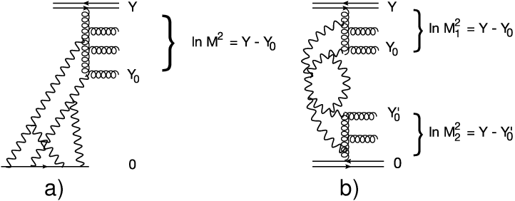
Therefore, we face the difficult problem of summing enhanced diagrams in the framework of the BFKL Pomeron calculus [17]. The goal of this paper is to sum all enhanced diagrams for dipole-dipole scattering at high energy. For solution of this problem we are going to exploit Mueller-Patel-Salam-Iancu (MPSI) approximation[18] shown in Fig. 2, following the procedure suggested in Ref.[19]. One can see that the MPSI approximation is based on two key features of high density QCD: on $t$-channel unitarity and on the simple dipole cascade generated by dilute system (one upper or lower dipole in our case). This cascade can be described by the simple generating functional [20, 21] which is equivalent to Balitsky-Kovchegov[4] and JIMWLK(KLWMIG)[5] evolutions. In the BFKL Pomeron calculus this cascade corresponds to summation of fan Pomeron diagrams in the region of $Y-Y^{\prime}\,\,\gg\,\,1$ and $Y^{\prime}-0\,\,\gg\,\,1$ in Fig. 2). Rapidity $Y^{\prime}$ is artificial rapidity which does not enter the final answer. Indeed, the BFKL Pomeron has the following property from the $t$-channel unitarity [1, 22] at any value of $Y^{\prime}$:

In Eq. (1.3) $N_{I\!\!P}$ describes the dipole-dipoles scattering amplitude due to the single BFKL Pomeron exchange, $G_{I\!\!P}$ denotes the Green function of the BFKL Pomeron. $\gamma\left(r_{1},r_{2},\vec{b}_{1}-\vec{b}_{2}\right)$ is the amplitude of interaction of two dipoles with sizes: $r_{1}$ and $r_{2}$ at the impact parameter $\vec{b}_{1}-\vec{b}_{2}$ in the Born Approximation of perturbative QCD in which two dipoles interact due to exchange of two gluons. $r$ and $R$ are the sizes of the scattering dipoles.

In the next section we will find the amplitude for dipole-dipole scattering (or the resulting Green function of the BFKL Pomeron) at high energy using the approach proposed in Ref.[23].

.

Most of the material of this section is not new and has already appeared in [23, 24]. We include it here for completeness in order to present a coherent picture of the approach.

Eq. (2.28) we can find in MPSI approximation [18, 19, 29] the scattering amplitude of two dipoles with sizes $r$ and $R$ and impact parameter $b$ which gives us the Green function of the dressed (final) BFKL Pomeron (see Fig. 3-b). It takes the form (see Fig. 2)

Eq. (3.31) can be re-written , using Eq. (1.3) in the form (see Fig. 3 for notations):

From Eq. (2.30) we derive the approximate simple formula for $N\left(Y-Y_{0},r,R,b\right)$ which looks as follows

where $\Gamma\left(0,T\right)$ is incomplete Euler gamma-function (see Ref. [36] formulae 8.35) and

Let us discuss the most difficult problem of CGC/saturation approach[30]: the impact parameter dependence of the Pomeron Green Function. For our simplified kernel which coincide with the DGLAP kernel outside of the saturation region, we can factorize out the non-perturbative large $b$ behaviour writing for the scattering amplitude in the form:

where $N_{0}$ is a constant (see Ref. [31]). In our estimates we choose $r=R=1/m$.

Indeed, considering the scattering amplitude at fixed transferred momentum $q$ ( which is Fourier conjugated to $b$), one can see that for $q\,<\,\mu_{soft}$ the evolutions in $ln(1/r)$ do not depend on $q$. However, for $q\,>\,\mu_{soft}$ the logs take the form $\ln\left(1/\left(rq\right)\right)$ and the $q$ dependence cannot be absorbed in $S\left(b\right)$ in Eq. (3.35)[31]. Using Eq. (3.35) we can absorbed the non-perturbative corrections at large $b$ in the definition of the saturation scale $Q_{s}\left(Y;b\right)$[32, 23, 17, 33, 34]. $S\left(b\right)$ is a non-perturbative form factor which we parameterize in the form

introducing mass $m$. Using the experimental data on cross section off the double parton interaction (see Eq. (1.1)) we can write that (see Fig. 6)

Eq. (3.37) is written assuming that only Pomeron loops contribute to the double parton interaction (see Fig. 6). This assumption looks natural in CGC/saturation approach for the proton-proton scattering as has been discussed in the introduction but, being phenomenological, it should be re-check in the future description of proton-proton date based on the result of this paper. Plugging the experimental value $\sigma_{eff}\,=\,12\,\div\,15\,mb$ we obtain $m\,=\,0.86\,\div\,1\,GeV$. This value of $m$ is in a good agreement with other indications of the second dimensional scale in the proton [35]. The variable $z$ in Eq. (3.35) is defined as $z\,\,=\,\,4\bar{\alpha}_{S}\,\left(Y-Y_{0}\right)\,+\,\ln\left(r^{2}/R^{2}\right)$. Collecting Eq. (3.35) and Eq. (3.36) the Pomeron Green function takes the following form

In all our numerical estimates we take $r=R=1/m$ and $N_{0}=1/2$. It should be mentioned that any other choice will lead only to redefinition of the value for $N_{0}$ in Eq. (3.38). With our choice we have

Certainly $N_{I\!\!P}\left(b=0,z=0,\right)=0.08\,\,\ll\,\,1$ satisfies the condition, that we have used obtaining the solution to the non-linear equation.

The equation for the diffractive production in dipole-target scattering (see Fig. 7) has been known for more than decade[37] (see also Ref.[6]). It has the same form as BK equation but for the following amplitude

The cross section of diffractive production with the rapidity gap ($Y-\ln M^{2}$ in Fig. 7) larger than $Y_{0}$ can be written through $N^{D}\left(Y,Y_{0},r,b\right)$ :

From Eq. (4.41)and unitarity constraint follows that $G\left(Y;Y_{0},r,b\right)$ is the inelastic cross section cross section of all processes except the diffractive production with the rapidity gap $\geq\,Y_{0}$. At $Y=Y_{0}$

where $N^{2}$ is the elastic cross section. Eq. (4.42) determines the initial condition for the equation for $G\left(Y;Y_{0},r,b\right)$. Since the equation for $G$ is the same as for $N$, therefore, the solution in the saturation region is equal to $G\left(z,z_{0}\right)\,\,=\,\,1-\exp\left(-\phi\left(z\right)\right)$ where $\phi$ is given by Eq. (2.22). The difference is the initial condition is given by Eq. (4.42) at $Y=Y_{0}$. Here, we consider the case when both $Y$ and $Y_{0}$ are so large that we have the geometric scaling behaviour for the amplitude both at $Y_{0}$ and $Y$, We introduce two variables

where $r$ and $r^{\prime}$ are the sizes of the dipoles with rapidities $Y$ and $Y_{0}$, respectively.

Rewriting the initial conditions in the variables of Eq. (4.43) we have

Final solution takes the form

and

In Fig. 8 we plot the total and diffraction cross sections. We fix $N_{pom}$ in Eq. (3.38) considering $N_{0}=0.5$. Using this form of $N_{I\!\!P}$ and solution of Eq. (2.25) we can calculate

In Fig. 9 we plot $\Delta\left(z_{0},b\right)-z_{0}$ versus $z_{0}$ and $b$. One can see that at small $z_{0}$ Eq. (4.44) can be re-written in the form

leading to $\Delta\left(z_{0}\right)-z_{0}\,=\,2\ln 2$ for $\bar{\alpha}_{S}=0.25$. From Eq. (4.47) we can calculate $M^{2}d\sigma_{diff}/d\ln M^{2}$ (see Fig. 7) which takes the form

In Fig. 10 we plot $\frac{d\sigma_{diff}}{d\ln M^{2}\,db}$ at fixed $z=17.75$ which for $\bar{\alpha}_{S}=0.25$ corresponds to the LHC energy. One can see that the largest contribution stems from the large mass kinematic region and the $b$-dependence shows a peripheral - type of behaviour versus $b$ with maximum at $b\approx 6$. We plot in this figure the elastic cross section at fixed $b$ ( $A^{2}_{el}(b)$) to illustrate the peripheral character of the diffraction production.

The pattern of calculation of diffractive production in the dipole-dipole scattering is shown in Fig. 11.This picture illustrates the main difference between calculation of the scattering amplitude and the cross section of the diffractive production: for the latter we need to introduce the difference between BFKL Pomerons in the scattering amplitude (in black in Fig. 11 and in the complex conjugated amplitude shown in blue in Fig. 11 (see Ref. [6, 38] and references therein). The general equation for the cross section of the single diffractive production takes the form

where $\widetilde{G}$ denotes the Pomeron Green’s function in the complex conjugated amplitude ($N^{*}$) and $C^{D}_{n-k,k}$ and $C_{n}$ are the coefficients in the series:

As has been shown in Ref.[38] we need to re-write Eq. (4.45) and Eq. (4.46) in the following form to obtain coefficients $C^{D}_{n-k,k}$

Using Eq. (5.52) and Eq. (5.53) we can simplify Eq. (5.51) reducing it to the form:

leading to $C^{D}_{n-k,k}\,\,=\,\,\frac{n!}{(n-k)!k!}C^{D}_{n}$. Note, that two first terms in Eq. (5.53) do not contribute to Eq. (5.50).

Performing summation over $n$ and $k$ in Eq. (5.51) we use for $N$ the approximate expression of Eq. (2.30) which we re-write in the following form

References

- [1] L. V. Gribov, E. Levin and M. G. Ryskin, Phys. Rep. 100 (1983) 1.
- [2] A. H. Mueller and J. Qiu, Nucl. Phys. B268 (1986) 427.
- [3]
L. McLerran and R. Venugopalan,
Phys. Rev. D49 (1994) 2233, 3352; D50 (1994) 2225;
D53 (1996) 458;
D59 (1999) 09400. - [4] I. Balitsky, Nucl. Phys. B463 (1996) 99; Y. Kovchegov, Phys. Rev. D60 (2000) 034008.
- [5] J. Jalilian-Marian, A. Kovner, A. Leonidov and H. Weigert, Phys. Rev. D59, 014014 (1998), [arXiv:hep-ph/9706377]; Nucl. Phys. B504, 415 (1997), [arXiv:hep-ph/9701284]; J. Jalilian-Marian, A. Kovner and H. Weigert, Phys. Rev. D59, 014015 (1999), [arXiv:hep-ph/9709432]; A. Kovner, J. G. Milhano and H. Weigert, Phys. Rev. D62, 114005 (2000), [arXiv:hep-ph/0004014] ; E. Iancu, A. Leonidov and L. D. McLerran, Phys. Lett. B510, 133 (2001); [arXiv:hep-ph/0102009]; Nucl. Phys. A692, 583 (2001), [arXiv:hep-ph/0011241]; E. Ferreiro, E. Iancu, A. Leonidov and L. McLerran, Nucl. Phys. A703, 489 (2002), [arXiv:hep-ph/0109115]; H. Weigert, Nucl. Phys. A703, 823 (2002), [arXiv:hep-ph/0004044].
- [6] Yuri V Kovchegov and Eugene Levin, “ Quantum Choromodynamics at High Energies”, Cambridge Monographs on Particle Physics, Nuclear Physics and Cosmology, Cambridge University Press, 2012 and references therein.
- [7] E. Levin and A. H. Rezaeian, Phys. Rev. D 83 (2011) 114001 [arXiv:1102.2385 [hep-ph]], AIP Conf. Proc. 1350 (2011) 243 [arXiv:1011.3591 [hep-ph]], Phys. Rev. D 82 (2010) 054003 [arXiv:1007.2430 [hep-ph]], Phys. Rev. D 82 (2010) 014022 [arXiv:1005.0631 [hep-ph]]; P. Tribedy and R. Venugopalan, Nucl. Phys. A 850 (2011) 136 [Erratum-ibid. A 859 (2011) 185] [arXiv:1011.1895 [hep-ph]].
- [8] E. Levin and A. H. Rezaeian, Phys. Rev. D 84 (2011) 034031 [arXiv:1105.3275 [hep-ph]]; K. Dusling and R. Venugopalan, Phys. Rev. Lett. 108, 262001 (2012) [arXiv:1201.2658 [hep-ph]], “Evidence for BFKL and saturation dynamics from di-hadron spectra at the LHC,” arXiv:1210.3890 [hep-ph]. A. Kovner and M. Lublinsky , “Angular and long range rapidity correlations in particle production at high energy,” arXiv:1211.1928 [hep-ph] and references therein.
- [9] W. Li, Mod. Phys. Lett. A 27 (2012) 1230018 [arXiv:1206.0148 [nucl-ex]], V. Khachatryan et al. [CMS Collaboration], JHEP 1009 (2010) 091 [arXiv:1009.4122 [hep-ex]].
- [10] S. Chatrchyan et al. [CMS Collaboration], Phys. Lett. B 718 (2013) 795 [arXiv:1210.5482 [nucl-ex]], B. Abelev et al. [ ALICE Collaboration], arXiv:1212.2001 [nucl-ex], G. Aad et al. [ATLAS Collaboration], arXiv:1212.5198 [hep-ex].
- [11] A. Adare et al. [PHENIX Collaboration], Phys. Rev. C 78 (2008) 014901 [arXiv:0801.4545 [nucl-ex]], B. I. Abelev et al. [STAR Collaboration], Phys. Rev. C 80 (2009) 064912 [arXiv:0909.0191 [nucl-ex]], B. Alver et al. [PHOBOS Collaboration], Phys. Rev. Lett. 104 (2010) 062301 [arXiv:0903.2811 [nucl-ex]], S. Chatrchyan et al. [CMS Collaboration], Phys. Rev. Lett. 109 (2012) 022301 [arXiv:1204.1850 [nucl-ex]], Eur. Phys. J. C 72 (2012) 2012 [arXiv:1201.3158 [nucl-ex]], G. Aad et al. [ATLAS Collaboration], Phys. Rev. C 86 (2012) 014907 [arXiv:1203.3087 [hep-ex]], Phys. Rev. Lett. 105 (2010) 252303 [arXiv:1011.6182 [hep-ex]], K. Aamodt et al. [ALICE Collaboration], Phys. Lett. B 708 (2012) 249 [arXiv:1109.2501 [nucl-ex]].
- [12] G. Aad et al. [ATLAS Collaboration], New J. Phys. 15 (2013) 033038 [arXiv:1301.6872 [hep-ex]], V. M. Abazov et al. [D0 Collaboration], Phys. Rev. D 81 (2010) 052012 [arXiv:0912.5104 [hep-ex]], F. Abe et al. [CDF Collaboration], Phys. Rev. D 47 (1993) 4857, Phys. Rev. D 56 (1997) 3811, J. Alitti et al. [UA2 Collaboration], Phys. Lett. B 268 (1991) 145, T. Akesson et al. [Axial Field Spectrometer Collaboration], Z. Phys. C 34, 163 (1987).
- [13] E. Gotsman, E. Levin and U. Maor, Phys. Lett. B 716 (2012) 425 [arXiv:1208.0898 [hep-ph]].
- [14] K. Aamodt et al. [ALICE Collaboration], Eur. Phys. J. C 68 (2010) 89 [arXiv:1004.3034 [hep-ex]], JHEP 1002 (2010) 041 [arXiv:1002.0621 [hep-ex]], G. Aad et al. [ATLAS Collaboration], Phys. Lett. B 688 (2010) 21 [arXiv:1003.3124 [hep-ex]].
- [15] E. A. Kuraev, L. N. Lipatov, and F. S. Fadin, Sov. Phys. JETP 45, 199 (1977); Ya. Ya. Balitsky and L. N. Lipatov, Sov. J. Nucl. Phys. 28, 22 (1978).
- [16] L. N. Lipatov, Phys. Rep. 286 (1997) 131; Sov. Phys. JETP 63 (1986) 904 [Zh. Eksp. Teor. Fiz. 90, 1536 (1986)].
- [17] M. A. Braun, Phys.Lett. B 483 (2000) 115, [arXiv:hep-ph/0003004]; Eur.Phys.J C 33 (2004) 113 [arXiv:hep-ph/0309293] ; Eur. Phys. J. C 16, 337 (2000) [hep-ph/0001268], Phys. Lett. B 632 (2006) 297, [Eur. Phys. J. C 48 (2006) 511], [arXiv:hep-ph/0512057], Eur. Phys. J. C 33 (2004) 113 [hep-ph/0309293], Eur. Phys. J. C 16, 337 (2000) [hep-ph/0001268].
- [18] A. H. Mueller and B. Patel: Nucl. Phys. B425 (1994) 471; A. H. Mueller and G. P. Salam: Nucl. Phys. B475, (1996) 293; G. P. Salam: Nucl. Phys. B461 (1996) 512; E. Iancu and A. H. Mueller: Nucl. Phys. A730 (2004) 460.
- [19] E. Levin, J. Miller and A. Prygarin, Nucl. Phys. A 806 (2008) 245 [arXiv:0706.2944 [hep-ph]].
- [20] A. H. Mueller, Nucl. Phys. B 415, 373 (1994); Nucl. Phys. B 437 (1995) 107 [arXiv:hep-ph/9408245].
- [21] E. Levin and M. Lublinsky, Nucl. Phys. A 730, 191 (2004) [hep-ph/0308279]; Phys. Lett. B 607 (2005) 131 [hep-ph/0411121].
- [22] A. H. Mueller and A. I. Shoshi, Nucl. Phys. B 692 (2004) 175 [arXiv:hep-ph/0402193].
- [23] E. Levin and K. Tuchin, Nucl. Phys. B 573 (2000) 833 [arXiv:hep-ph/9908317].
- [24] A. Kormilitzin, E. Levin and S. Tapia, Nucl. Phys. A 872 (2011) 245 [arXiv:1106.3268 [hep-ph]].
- [25]
V. N. Gribov and L. N. Lipatov, Sov. J. Nucl. Phys 15 (1972)
438;
G. Altarelli and G. Parisi, Nucl. Phys. B 126 (1977) 298;
Yu. l. Dokshitser, Sov. Phys. JETP 46 (1977) 641. - [26] E. Iancu, K. Itakura and L. McLerran, Nucl. Phys. A 708 (2002) 327 [hep-ph/0203137]; A. H. Mueller and D. N. Triantafyllopoulos, Nucl. Phys. B 640 (2002) 331 [hep-ph/0205167]; D. N. Triantafyllopoulos, Nucl. Phys. B 648 (2003) 293 [hep-ph/0209121].
- [27] J. Bartels, E. Levin, Nucl. Phys. B387 (1992) 617; A. M. Stasto, K. J. Golec-Biernat, J. Kwiecinski, Phys. Rev. Lett. 86 (2001) 596, [hep-ph/0007192]; L. McLerran, M. Praszalowicz, Acta Phys. Polon. B42 (2011) 99, [arXiv:1011.3403 [hep-ph]] B41 (2010) 1917, [arXiv:1006.4293 [hep-ph]]. M. Praszalowicz, [arXiv:1104.1777 [hep-ph]], [arXiv:1101.0585 [hep-ph]].
- [28] Andrei D. Polyanin and Valentin F. Zaitsev, “ Handbook of nonlinear Partial Differential Equations”, Chapman & Hall/CRC, 2004.
- [29] M. Kozlov and E. Levin, Nucl. Phys. A 739 (2004) 291 [hep-ph/0401118].
- [30] A. Kovner and U. A. Wiedemann, Phys. Rev. D 66, 051502, 034031 (2002) [hep-ph/0112140,hep-ph/0204277]; Phys. Lett. B 551, 311 (2003) [hep-ph/0207335].
- [31] E. Gotsman, E. Levin, M. Lublinsky, U. Maor and K. Tuchin, Nucl. Phys. A 697, 521 (2002).
- [32] A. H. Mueller, Nucl. Phys. B 335, 115 (1990).
- [33] N. Armesto and M. A. Braun, Eur. Phys. J. C 20, 517 (2001) [hep-ph/0104038].
- [34] M. Lublinsky, E. Gotsman, E. Levin and U. Maor, Nucl. Phys. A 696, 851 (2001) [hep-ph/0102321]; M. Lublinsky, Eur. Phys. J. C 21, 513 (2001) [hep-ph/0106112].
- [35] B. Z. Kopeliovich, I. K. Potashnikova, B. Povh and I. Schmidt, Phys. Rev. D 76 (2007) 094020 [arXiv:0708.3636 [hep-ph]].
- [36] I. Gradstein and I. Ryzhik, Table of Integrals, Series, and Products, Fifth Edition, Academic Press, London, 1994.
- [37] Y. V. Kovchegov and E. Levin, Nucl. Phys. B 577, 221 (2000) [hep-ph/9911523].
- [38] A. Kormilitzin, E. Levin and A. Prygarin, Nucl. Phys. A 813 (2008) 1 [arXiv:0807.3413 [hep-ph]]; E. Levin and A. Prygarin, Eur. Phys. J. C 53 (2008) 385 [hep-ph/0701178].
- [39] Y. V. Kovchegov and K. Tuchin, Phys. Rev. D 65 (2002) 074026 [hep-ph/0111362].
- [40] T. Altinoluk, C. Contreras, A. Kovner, E. Levin, M. Lublinsky and A. Shulkin, “QCD Reggeon Calculus From KLWMIJ/JIMWLK Evolution: Vertices, Reggeization and All,” arXiv:1306.2794 [hep-ph].