Group-Sparse Signal Denoising: Non-Convex Regularization, Convex Optimization
Abstract
Convex optimization with sparsity-promoting convex regularization is a standard approach for estimating sparse signals in noise. In order to promote sparsity more strongly than convex regularization, it is also standard practice to employ non-convex optimization. In this paper, we take a third approach. We utilize a non-convex regularization term chosen such that the total cost function (consisting of data consistency and regularization terms) is convex. Therefore, sparsity is more strongly promoted than in the standard convex formulation, but without sacrificing the attractive aspects of convex optimization (unique minimum, robust algorithms, etc.). We use this idea to improve the recently developed ‘overlapping group shrinkage’ (OGS) algorithm for the denoising of group-sparse signals. The algorithm is applied to the problem of speech enhancement with favorable results in terms of both SNR and perceptual quality.
I Introduction
In this work, we address the problem of estimating a vector from an observation ,
| (1) |
where is additive white Gaussian noise (AWGN). We assume that is a group-sparse vector. By group-sparse, we mean that large magnitude values of tend not to be isolated. Rather, large magnitude values tend to form clusters (groups). Furthermore, we do not assume that the group locations are known, nor that the group boundaries are known. In fact, we do not assume that the groups have well defined boundaries. An example of such a vector (in 2D) is the spectrogram of a speech waveform. The spectrogram of a speech waveform exhibits areas and ridges of large magnitude, but not isolated large values. The method proposed in this work will be demonstrated on the problem of speech filtering.
Convex and non-convex optimization are both common practice for the estimation of sparse vectors from noisy data [1]. In both cases one often seeks the solution to the problem
where is the regularization (or penalty) term and . Convex formulations are advantageous in that a wealth of convex optimization theory can be leveraged and robust algorithms with guaranteed convergence are available [8]. On the other hand, non-convex approaches are advantageous in that they usually yield sparser solutions for a given residual energy. However, non-convex formulations are generally more difficult to solve (due to suboptimal local minima, initialization issues, etc.). Also, solutions produced by non-convex formulations are generally discontinuous functions of input data (e.g., the discontinuity of the hard-threshold function).
Generally, convex approaches are based on sparsity-promoting convex penalty functions (e.g., the norm), while non-convex approaches are based on non-convex penalty functions (e.g., the pseudo-norm with [39], re-weighted / [10, 61]). Other non-convex algorithms seek sparse solutions directly (e.g., OMP [40], iterative hard thresholding [6, 34, 51, 25], and greedy [37]).
In this work, we take a different approach, proposed by Blake and Zimmerman [5] and by Nikolova [43]. Namely, the use of a non-convex non-smooth penalty function chosen such that the total cost function (consisting of data consistency and regularization terms) is strictly convex. This is possible “by balancing the positive second derivatives in the [data consistency term] against the negative second derivatives in the [penalty] terms” [5, page 132]. This idea has been further extended by Nikolova et al. [46, 44, 47, 48].
The contribution of this work relates to (1) the formulation of the group-sparse denoising problem as a convex optimization problem albeit defined in terms of a non-convex penalty function, and (2) the derivation of a computationally efficient iterative algorithm that monotonically reduces the cost function value. We utilize non-convex penalty functions (in fact, concave on the positive real line) with parametric forms; and we identify an interval for the parameter that ensures the strict convexity of the total cost function, . As the total cost function is strictly convex, the minimizer is unique and can be obtained reliably using convex optimization techniques. The algorithm we present is derived according to the principle of majorization-minimization (MM) [24]. The proposed approach:
- 1.
promotes sparsity more strongly than any convex penalty function can,
- 2.
is translation invariant (due to groups in the proposed method being fully overlapping),
- 3.
is computationally efficient ( per iteration) with decreasing cost function, and
- 4.
requires no algorithmic parameters (step-size, Lagrange, etc.).
We demonstrate below that the proposed approach substantially improves upon our earlier work that considered only convex regularization [13].
I-A Related Work
The estimation and reconstruction of signals with group sparsity properties has been addressed by numerous authors. We make a distinction between two cases: non-overlapping groups [64, 36, 35, 21, 12] and overlapping groups [33, 19, 23, 32, 2, 3, 50, 1, 41, 63, 14]. The non-overlapping case is the easier case: when the groups are non-overlapping, there is a decoupling of variables, which simplifies the optimization problem. When the groups are overlapping, the variables are coupled. In this case, it is common to define auxiliary variables (e.g., through the variable splitting technique) and apply methods such as the alternating direction method of multipliers (ADMM) [7]. This approach increases the number of variables (proportional to the group size) and hence increases memory usage and data indexing. In previous work we describe the ‘overlapping group shrinkage’ (OGS) algorithm [13] for the overlapping-group case that does not use auxiliary variables. The OGS algorithm exhibits favorable asymptotic convergence in comparison with algorithms that use auxiliary variables [13, Fig. 5]. In comparison with previous work on convex optimization for overlapping group sparsity, including [13], the current work promotes sparsity more strongly. The current work extends the OGS algorithm to the case of non-convex regularization, yet remains within the convex optimization framework.
As noted above, the balancing of the data consistency term and the penalty term, so as to formulate a convex problem with a non-convex penalty term, was described in Refs. [5, 43] and extended in [46, 44, 47, 48]. This approach was used to initialize a scheme named ‘graduated non-convexity’ (GNC) in [5]. The goal of GNC is to minimize a non-convex function by minimizing a sequence of functions . The first one is a convex approximation of , and the subsequent ones are non-convex and progressively similar to . In order that the initial approximation of be convex, the penalty function must satisfy an eigenvalue condition [5]. A looser condition, which promotes sparsity more strongly, can be expressed as a semidefinite program (SDP), but this incurs a higher computational cost [57]. In the method described here, we use the same balancing idea as in GNC; however, our goal is to minimize a convex function, not a non-convex one as in GNC. In particular, we use the balancing idea to construct a convex function that maximally promotes sparsity, and we seek to subsequently solve this convex problem. We note that here our primary goal is to capture group sparsity behavior, which is not considered in the GNC work. We also note that the computationally demanding SDP arising in Ref. [57] does not arise in the current work. The algorithm developed here is computationally simple.
II Preliminaries
II-A Notation
We will work with finite-length discrete signals which we denote in lower case bold. The -point signal is written as
We use the notation
| (2) |
to denote the -th group of vector of size . We consistently use (a positive integer) to denote the group size. At the boundaries (i.e., for and ), some indices of fall outside . We take these values as zero; i.e., for , we take .
We denote the non-negative real line as and the positive real line as . Given a function , the left-sided and right-sided derivatives of at are denoted and , respectively. The notation denotes set difference; i.e., .
II-B Penalty Functions
We will make the following assumptions on the penalty function, .
- 1.
is continuous on .
- 2.
is twice differentiable on .
- 3.
(symmetric)
- 4.
(increasing on )
- 5.
(concave on )
- 6.
(unit slope at zero)
- 7.
(maximally concave at zero)
We will utilize penalty functions parameterized by a scalar parameter, . We use the notation to denote the parameterized form.
Examples of parameterized penalty functions satisfying the assumptions above are the logarithmic penalty,
| (3) |
the arctangent penalty [57],
| (4) |
and the first order rational function [28]
| (5) |
The rational penalty is defined for . The log and atan penalties are defined for . Note that as , the three penalty functions approach the absolute value function. They are illustrated in Fig. 1.
For later use, we record the value of the right-sided second derivative of the three penalty functions:
| (6) |
Note that the pseudo-norm (), i.e., , does not satisfy the above assumptions. It does not have unit slope at zero nor can it be normalized or scaled to do so.

II-C Threshold Functions
Proximity operators are a fundamental tool in efficient sparse signal processing [17, 16]. In the scalar case, proximity operators are thresholding/shrinkage function derived using a convex penalty function. In this work, we utilize non-convex penalty functions; however, we can still define a threshold function similar to the definition of a proximity operator. The following proposition is closely related to Lemma 3.1 in [42] and Theorem 3.3 in [45], both of which analyze the behavior of for non-smooth, not necessarily convex, .
Proposition 1.
Define by
| (7) |
where , , and satisfies the assumptions in Sec. II-B. Suppose also that is strictly convex. If , then the unique minimizer of is zero. That is, is a threshold function and is the threshold value.
Proof.
This is a special case of Proposition 3 wherein is a multivariate threshold function, . ∎
Figure 2 illustrates threshold functions corresponding to several penalty functions. We use and . The threshold function corresponding to the absolute value penalty function is called the soft threshold function [20]. Notice that, except for the soft threshold function, the threshold functions approach the identity function. The atan threshold function approaches identity the fastest.
The fact that the soft threshold function reduces large values by a constant amount is considered its deficiency. In the estimation of sparse signals in AWGN, this behavior results in a systematic underestimation (bias) of large magnitude signal values [22]. Hence, threshold functions that are asymptotically unbiased are often preferred to the soft threshold function, and the penalty functions from which they are derived promote sparsity more strongly than the norm [10, 11, 27, 26]. The atan penalty function is derived specifically for its favorable behavior in this regard [57].
As shown in Ref. [57], if satisfies the above assumptions, then the right-sided derivative of at the threshold is given by
| (8) |
Hence, with parameters and , we use (6) to find that for , , and . That is, each of these threshold functions in Fig. 2 have the same derivative at , but they approach the identity at different rates.

III OGS with non-convex regularization
For denoising group-sparse signals in AWGN, we propose to minimize the cost function, ,
| (9) |
where is a (non-convex) sparsity promoting penalty function satisfying the assumptions in Sec. II-B, and . The group size, (a positive integer), should be selected based on the size of the groups (clusters) arising in the data. This constitutes one’s ‘prior knowledge’ regarding the group sparsity behavior of the data and may need to be obtained through some trial-and-error.
In order to leverage convex optimization principles and avoid non-convex optimization issues (local minima, sensitivity to noise, etc.), we seek to restrict so that is strictly convex. We note that the minimization of is not so straight forward. First, all the variables are coupled due to the overlapping group structure of the regularization term. That is, each component depends on every data sample (albeit the influence diminishes with distance ). Secondly, is not differentiable. In particular, is generally not differentiable at the minimizer, , due to the sparsity of induced by the regularizer. (The penalty function, , is non-differentiable at zero). For these reasons, it is desirable that be strictly convex.
In the following, we address the questions:
- 1.
For what values of is strictly convex?
- 2.
When is strictly convex, how can the unique minimizer, , be efficiently computed?
First, we make a few remarks. If , then simplifies to
| (10) |
the components are not coupled, and the minimization of amounts to component-wise non-linear thresholding; i.e., . In this case, the cost function does not promote any group structure.
If is the absolute value function, i.e., , then the cost function in (9) is the same cost function considered in our earlier work [13], which considers only convex regularization.
If and is the absolute value function, then the minimizer of is given by point-wise soft thresholding of .
The current work addresses the case and a non-convex regularizer, so as to promote group sparsity more strongly in comparison to convex regularization. The enhanced sparsity will be illustrated in Example 1 in Sect. IV-A.
We also have the following result, similar to lemma 1 of Ref. [63] which considered convex regularizers promoting group sparsity.
Lemma 1.
Proof.
1) Define and . Given , define as for , and for . For each group , we have . Since is increasing for , we have . Therefore, for all ,
This implies for .
2) Proof by contradiction. Suppose , but for some . Define by , and for . It can be shown as in 1) that . This contradicts the optimality of .
3) The proof is like 2).
4) Proof by contradiction. Suppose , but for some . Define by , and for . It can shown as in 1) that . This contradicts the optimality of . Together with 2), it follows that if , then . Similarly, if , then . ∎
III-A Group Thresholding
In order to determine the convexity of , we first consider a simpler cost function, , which consists of a single group. What values of ensure that is strictly convex?
Proposition 2.
Consider the functions and , defined as
| (11) | ||||
| (12) |
where , , , and satisfies the assumptions in Sec. II-B. Then is strictly convex iff is strictly convex. Furthermore, if
| (13) |
then and are both strictly convex.
Proof.
Let us expand and as
| (14) | ||||
| (15) |
Define and ,
| (16) | ||||
| (17) |
It can be observed that is strictly convex iff is strictly convex. Similarly is strictly convex iff is.
We claim that is strictly convex if and only if the function is strictly convex. [Note that .]
Suppose is strictly convex. From (17), is increasing on . Based on the convexity of and Proposition 2.1.7 of Ref. [30, page 89], is strictly convex, and hence is strictly convex.
Suppose is strictly convex. Given , define and with . Note that in (17) is symmetric. For all satisfying and , we have
which implies the strict convexity of .
To prove the second part of this proposition, according to the assumptions on in Sec. II-B, is continuous on , twice differentiable on , and symmetric. Hence, from Corollary 3 (see Appendix), it is sufficient that be positive on and that .
Note that ; and by symmetry . Hence .
To ensure the second derivative of is positive on , we have the condition
| (18) |
or
| (19) |
Due to assumption 7 on [i.e., ], we have (13). ∎
The condition (13) can be used to determine values of that ensure strict convexity of . For the log, atan, and rational penalty functions (, , ), we use (6) to obtain the following intervals for ensuring strict convexity of .
Corollary 1.
Suppose is one of the penalty functions given in Sec. II-B (, , ). Then is strictly convex if
| (20) |
Based on a strictly convex function , we may define a multivariate threshold/shrinkage function as in the scalar case (7). It is informative to note the threshold of the multivariate thresholding function.
Proposition 3.
Define by
| (21) |
where , and satisfies the assumptions in Sec. II-B. Suppose also that is strictly convex. If , then the unique minimizer of is the zero vector. That is, is a multivariate threshold function with threshold .
Proof.
We consider the subgradient of a convex function (see Ref. [30, Definition 1.1.4, page 165]), denoted by , is equal to . Since by assumption 6 in Sec. II-B, we have , which is equal to .
This leads to
| (22) |
Since is a minimizer of iff (see [30, Theorem 2.2.1, page 177]), we deduce the following.
- •
Suppose . We can choose satisfying such that . We have , which implies that is the minimizer of .
- •
Suppose . There is no satisfying such that . Hence, is not the minimizer of .
From the arguments above, we conclude that defines the threshold of . ∎
When is the absolute value function, the induced multivariate threshold function can be expressed in closed form [58]. (Essentially, it performs soft-thresholding on the 2-norm.) A generalization to the case where the data consistency term in (21) is of the form has also been addressed [52]. We note that neither [52] nor [58] consider either non-convex regularization or overlapping group sparsity.
If the penalty function, , is strictly concave on the positive real line (log, atan, etc.), then the induced multivariate threshold function results in less bias of large magnitude components; i.e., approaches the identity function for large . An exploration along these lines is given in [56]; however, in that work, the non-convexity was quite mild and not adjustable. (The non-convex regularization in [56] is based on the multivariate Laplace probability density function, which does not have a shape parameter, analogous to in the current work.) Furthermore, overlapping group sparsity is not considered in [56].
III-B Overlapping Group Thresholding
Using the results above, we can find a condition on to ensure in (9) is strictly convex. The result permits the use of non-convex regularization to strongly promote group sparsity while preserving strict convexity of the total cost function, .
Theorem 1.
Consider , defined as
| (23) |
where , , , and satisfies the assumptions in Sec. II-B. Then is strictly convex if
| (24) |
Proof.
Corollary 2.
Suppose is one of the penalty functions given in Sec. II-B (, , ). Then is strictly convex if
| (27) |
We give some practical comments on using (27) to set the parameters . We suggest that be chosen first, based on the structural properties of the signal to be denoised. We suggest that then be set to a fixed fraction of its maximal value; i.e., fix and set . So, we consider as a function of . We then set according to the noise variance. In Sec. III-E, we describe two approaches for the selection of . In our numerical experiments on speech enhancement, we have found that setting to its maximal value of generally yields the best results; i.e., . Hence, in the examples in Sec. IV, we set to its maximal value.
Equation (27) may suggest the proposed method becomes ineffective for large . It can be noted from (27) that for large , should be small (). If is set so as to achieve a desired degree of noise suppression, then (27) implies should be small. A small , in turn, limits the non-convexity of the regularizer. Hence, it appears the benefit of the proposed non-convex regularization method is diminished for large . However, two considerations offset this reasoning. First, for larger , a smaller value of is needed so as to achieve a fixed level of noise suppression (this can be seen, for example, in Table III). Secondly, for larger , there is greater overlap between adjacent groups because the groups are fully-overlapping; so, regularization may be more sensitive to .
III-C Minimization Algorithm
To derive an algorithm minimizing the strictly convex function in (9), we use the majorization-minimization (MM) procedure [24] as in [13]. The MM procedure replaces a single minimization problem by a sequence of (simpler) ones. Specifically, MM is based on the iteration
| (28) |
where the function, , is a majorizer (upper bound) of and is the iteration index. For to be a majorizer of it should satisfy
| (29) | ||||
| (30) |
The MM procedure monotonically reduces the cost function value at each iteration. Under mild conditions, the sequence converges to the minimizer of [24].
To specify a majorizer of the cost function in (9), we first specify a majorizer of the penalty function, . To simplify notation, we suppress the dependence of on .

Lemma 2.
Assume satisfies the assumptions in Sec. II-B. Then , defined by
| (31) |
is a majorizer of except for , i.e.,
| (32) | ||||
| (33) |
The majorization of by is illustrated in Fig. 3.
Proof.
By direct substitution, one may verify (33). We now show (32). Let and . Using Taylor’s theorem [55, Theorem 5.15], we have
| (34) |
for some between and . By the assumptions on , we have . Hence from (34),
| (35) |
Note that implies
| (36) |
Using (36) for on the left-hand side of (35) gives
| (37) |
Recognizing that the right-hand side of (37) is , we obtain for all , . By symmetry of and , we obtain (32). ∎
Since is a majorizer of , the function
| (38) |
is a majorizer of . Using (31), the function is given by
where does not depend on . After algebraic manipulations, can be expressed as
| (39) |
where is defined as
| (40) |
Note that the components in (39) are uncoupled. Furthermore, is quadratic in . Hence, the minimizer of with respect to is easily obtained. The quantities in (40) are readily computed; is essentially a double -point convolution, with a nonlinearity between the two convolutions.
| input: , , , | |||
| repeat | |||
| until convergence | |||
| return: |
For finite precision implementations only.
Using (39) in the MM iteration (28), we obtain
| (41) |
where is given by (40). This constitutes the OGS algorithm. The algorithm is summarized in Table I. We denote the output of the OGS algorithm as .
Note that in (31) is undefined if . This singularity issue often arises when a quadratic function is used to majorize a non-smooth function [49, 24]. This issue may manifest itself in the OGS algorithm whenever a -point group of is equal to the -point zero vector; i.e., if for some index and iteration . In the event of such an occurrence, the OGS algorithm would encounter a ‘divide-by-zero’ error. However, such an occurrence is guaranteed not to occur with suitable initialization, as described in [13]. For example, it is sufficient to initialize all to non-zero values, i.e., for all . With such an initialization, it is readily observed that in the denominator of (41) is strictly positive and finite and that for all and all iterations . When some components of the solution are zero (as expected, due to sparse regularization), those values approach zero in limit; i.e., as .
We propose initializing to ; i.e., , and we exclude from the iteration (41) those for which . The set in Table I serves to exclude these components from the iterative update. In this case, for all iterations , which is justified by part 1) of lemma 1. As a consequence of lemma 1, initializing to zero for is optimal. Therefore, the algorithm excludes these values from the update procedure because they are already optimal.
With the initialization , it is readily observed, as above, that in the denominator of (41) is strictly positive and finite and that for all and all iterations . Assuming infinite precision, it is sufficient to define prior to the loop only; the last line in Table I, indicated by , can be omitted. It is guaranteed that a division by zero will never occur, as discussed above.
The OGS algorithm proceeds by gradually attenuating the , , toward their optimal values (including zero). The attenuation is multiplicative, so the the value never equals zero, even though it may converge to zero. But if many values reach ‘machine epsilon’ then a divide by zero may subsequently occur in the implementation. Hence, to avoid possible divide-by-zero errors due to finite precision arithmetic, the OGS algorithm updates at the end of the loop in Table I. The small number, , may be set to ‘machine epsilon’, which for single precision floating point is about . This value is usually considered the same as zero.
We do not prove the convergence of the OGS algorithm to the minimizer of due to the complication of the singularity issue. However, due to its derivation based on the majorization-minimization principle, OGS is guaranteed to decrease the cost function at each iteration. Moreover, in practice, we have observed through extensive numerical investigation, that the algorithm has the same rapid convergence behavior as convex regularized OGS [13].
Note that in the OGS algorithm, summarized in Table I, the penalty function appears in only one place: the computation of . It can therefore be observed that the role of the penalty is encapsulated by the function . Table II lists this function for the penalty functions given in Sec. II-B. The function have very similar functional forms. The similarity of these functions reveal the close relationship among the listed penalty functions.
| penalty | ||
|---|---|---|
| abs | ||
| log | ||
| atan | ||
| rational |
III-D The Multidimensional Case
The results and algorithm described in the preceding sections can be extended to the multidimensional case straightforwardly. In the numerical experiments below, we use a two-dimensional version of the algorithm in order to denoise the time-frequency spectrogram of a noisy speech waveform.
Suppose is a 2D array of size ; i.e.,
The array can be expressed using multi-indices as
Let denote the size of a 2D group. Then a sub-group of size can be expressed as
In the two-dimensional case, the function in (9) is
| (42) |
and conditions (24) and (27) become
| (43) |
and
| (44) |
respectively. The algorithm in Table I is essentially the same for the two-dimensional case. The summations become double summations, etc. Extensions to higher dimensional signals is similarly straight forward.
III-E Regularization Parameter Selection
Noise level suppression. The regularization parameter, , can be selected using existing generic techniques such as the L-curve method. However, in [13] we described an approach to set based directly on the standard deviation, , of the AWGN, which we assume is known. This approach seeks to preserve one of the concepts of scalar thresholding (e.g., hard or soft thresholding), namely the processing of signal values based on relative magnitude. Consider the problem of estimating a sparse signal in AWGN. If many of the non-zero values of the sparse signal exceed the noise floor, then a suitable threshold value, , should exceed the noise floor. But should not be too large, or else the non-zero values of the sparse signal will be annihilated. Hence, it is reasonable to use the value . This threshold will set most of noise (about 99.7%) to zero. (If the sparse signal has non-zero values less than in magnitude, then those values will be lost.)
| , | |||||
|---|---|---|---|---|---|
This simplicity of this ‘three-sigma’ rule can not be leveraged so easily in the proposed OGS algorithm. However, we can still implement the concept of setting so as to reduce the noise down to a specified fraction of its original power. For this purpose, the effect of the OGS algorithm on pure zero-mean Gaussian noise, , can be measured through computation. In particular, the standard deviation of the OGS output as a function of can be found empirically and recorded. For example, Table III records the value
for several and group sizes . For this table we used the atan penalty function with set to its maximum value of ; i.e., . The value also depends on the number of iterations of the OGS algorithm. In computing Table III we have used a fixed number of 25 iterations.
We clarify how to use Table III to set the regularization parameter: Suppose in one-dimensional signal denoising, one seeks to set so that the OGS algorithm reduces down to . If one uses a group size of , the atan penalty function with , and 25 iterations, then according to Table III, one should use (see the last column of the fifth row of the table). For each group size , the table records a discrete set of pairs for . Linear interpolation on a -logarithmic scale can be used to estimate for other . For example, if one seeks to set so that the OGS algorithm reduces down to , then according to the interpolation illustrated in Fig. 4, one should use .

To set by this approach for other penalty functions, other values of , and for complex data, it is necessary to compute additional tables. We have precomputed a set of such tables to be available as supplementary material. Using precomputed tables and interpolation, a suitable value for can be found very quickly. These tables assume the noise is AWGN; for other noise models, other tables need to be precomputed. This approach is also effective for two-dimensional denoising (e.g., spectrogram denoising).
Monte-Carlo SURE. Another approach to select the regularization parameter, , is based on minimizing the mean square error (MSE). For the problem of denoising a signal in AWGN, the MSE is unknown in practice, due to the noise-free signal being unknown. But, the MSE can be estimated using Stein’s unbiased risk estimator (SURE) [60]. To estimate the MSE, SURE requires only the observation , noise variance , and divergence of the estimator. However, the computation of the divergence is intractable for many estimators, including OGS. To overcome this issue, it is proposed in Ref. [53] that Monte-Carlo methods be used. We have applied this approach, i.e., ‘Monte-Carlo SURE’ (MC-SURE), to estimate the MSE for complex-valued speech spectrogram denoising using OGS. Since the spectrogram is complex, we calculate the MS-SURE MSE by averaging real and imaginary divergences as in [9]. Figure 5 illustrates both the MSE, as calculated by MC-SURE, and the true MSE, as functions of . The estimated MSE is quite accurate, and the MSE-optimal value of is about 0.33. However, a disadvantage of MC-SURE is its high computational complexity. It requires two OGS optimizations for each to emulate the divergence.
It is noted in Ref. [53] that for non-smooth estimators, the MSE, as calculated by MC-SURE, tends to deviate randomly from the true MSE (see Fig. 4 in [53]). For OGS, the MSE calculated by MC-SURE closely follows the true MSE, as illustrated in Fig 5, which shows that OGS is close to continuous and bounded.

IV Experimental Results
IV-A Example 1: One-dimensional Signal Denoising
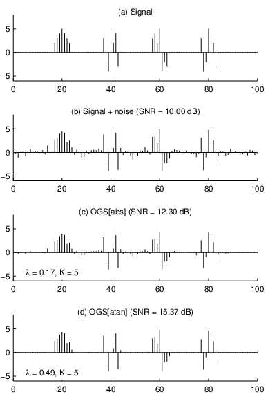
This example compares the proposed non-convex regularized OGS algorithm with the prior (convex regularized) version of OGS and with scalar thresholding. The SNRs are summarized in Table IV.
Figure 6a shows a synthetic group-sparse signal (same as in [13]). The noisy signal, shown in Fig. 6b, was obtained by adding white Gaussian noise (AWGN) with SNR of 10 dB. For each of soft and hard thresholding, we used the threshold, , that maximizes the SNR. The SNR values are summarized in the top row of Table IV.
| Estimator | |||||
| Param. | Hard thr. | Soft thr. | OGS[abs] | OGS[log] | OGS[atan] |
| max SNR | 13.84 | 12.17 | 12.30 | 14.52 | 15.37 |
| 6.74 | 3.86 | 8.01 | 12.07 | 13.92 | |
| 5.05 | 2.17 | 6.23 | 9.69 | 11.54 | |
| SNR is in dB; is the noise standard deviation. | |||||
The result obtained using the prior version of OGS [13] is shown in Fig 6c. This is equivalent to setting to the absolute value function; i.e. . So, we denote this as OGS[abs]. The result using the proposed non-convex regularized OGS is shown in Fig. 6d. We use the arctangent penalty function with set to the maximum value of that preserves convexity of ; i.e., we use . We denote this as OGS[atan]. We also used the logarithmic penalty (not shown in the figure). For each version of OGS, we used a group size of , and we set to maximize the SNR.
Comparing soft thresholding and OGS[abs] (both of which are based on convex regularization), it can be observed that OGS[abs] gives a higher SNR, but only marginally. Both methods leave residual noise, as can be observed for OGS[abs] in Fig. 6c. On the other hand, comparing OGS[atan] and OGS[abs], it can be observed that OGS[atan] (based on non-convex regularization) is substantially superior: it has a substantially higher SNR and almost no residual noise is visible in the denoised signal. Comparing OGS[log] and OGS[atan] with hard thresholding (see Table IV), it can be observed the new non-convex regularized OGS algorithm also yields higher SNR than hard thresholding. This example demonstrates the effectiveness of non-convex regularization for promoting group sparsity.
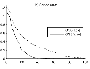
To more clearly compare the result of OGS[abs] and OGS[atan], these two results are shown together in Fig. 7. In Fig. 7a, the output value, , is shown versus the input value, , for . Compared to OGS[abs], the OGS[atan] algorithm better preserves the amplitude of the non-zero values of the original signal, while better thresholding small values. Figure 7b shows the denoising error for the two OGS methods. It can be observed that the denoised signal produced by OGS[atan] has much less error than OGS[abs]. (For OGS[atan], the error is essentially zero for 50% of the signal values.)
As a second experiment, we selected and for each method, so as to reduce the noise standard deviation, , down to , as described in Sec. III-E. The resulting SNRs, given in the second row of Table IV, are much lower. (This method does not maximize SNR, but it does ensure residual noise is reduced to the specified level.) The low SNR in these cases is due to the attenuation (bias) of large magnitude values. However, it can be observed that OGS, especially with non-convex regularization, significantly outperforms scalar thresholding.

IV-B Example 2: Speech Denoising
This example evaluates the use of the proposed OGS algorithm for the problem of speech enhancement (denoising). We compare the OGS algorithm with several other algorithms. For the evaluation, we use female and male speakers, multiple sentences, two noise levels, and two sampling rates.
Let denote the noisy speech waveform and denote the complex-valued short-time Fourier transform of . For speech enhancement, we apply the two-dimensional form of the OGS algorithm to and then compute the inverse STFT; i.e.,
with where and are the spectral and temporal widths of the two-dimensional group. We implement the STFT with 50% frame overlap and a frame duration of 32 milliseconds (e.g., 512 samples at sampling rate 16 kHz).
Throughout this example, we use the non-convex arctangent penalty function with set to its maximum value of . In all cases, we use a fixed number of 25 iterations within the OGS algorithm.
Each sentence in the evaluation is spoken by both a male and a female speaker. There are 15 sentences sampled at 8 kHz, and 30 sentences sampled at 16 kHz. The 8 kHz and 16 kHz signals were obtained from Ref. [38] and a Carnegie Mellon University (CMU) website, respectively.11 1 The CMU files were downloaded from http://www.speech.cs.cmu.edu/cmu_arctic/cmu_us_bdl_arctic/wav and http://www.speech.cs.cmu.edu/cmu_arctic/cmu_us_clb_arctic/wav. This evaluation used files arctic_a0001 - arctic_a0030. To simulate noisy speech, we added white Gaussian noise.
The time-frequency spectrogram of a noisy speech signal (arctic_a0001) with an SNR of 10 dB is illustrated in Fig. 8a. Figure 8b illustrates the result of OGS[atan] using group size ; i.e., eight spectral samples by two temporal samples. It can be observed that noise is effectively suppressed while details are preserved.
Figure 9 compares the proposed OGS[atan] algorithm with the prior version of OGS [13], i.e., OGS[abs]. The figure shows a single frame of the denoised spectrograms, corresponding to seconds. The prior and proposed OGS algorithms are illustrated in parts (a) and (b) respectively. In both (a) and (b), samples of the noise-free spectrogram, to be recovered, are indicated by dots. (The noisy spectrogram is not illustrated). Comparing (a) and (b), it can be observed that above 2 kHz, OGS[atan] estimates the noise-free spectrum more accurately than OGS[abs].
In terms of run-time, for a signal of length (i.e., 3.2 seconds at sampling rate of 16 kHz), algorithms OGS[abs] and OGS[atan] ran in 0.18 and 0.22 seconds, respectively. Timings were performed on a 2013 MacBook Pro (2.5 GHz Intel Core i5) running Matlab R2011a.
Regularization parameter. We have found empirically, that setting to maximize SNR yields speech with noticeable undesirable perceptual artifacts (‘musical noise’). This known phenomenon is due to residual noise in the STFT domain. Therefore, we instead set the regularization parameter, , using the noise suppression approach described in Sec. III-E. In particular, we set so as to reduce the noise standard deviation down to . We have selected this value so as to optimize the perceptual quality of the denoised speech according to informal listening tests. In particular, this value is effective at suppressing the ‘musical noise’ artifact. We also note that this approach leads to greater regularization (higher ) than SNR-optimization of .


Group size. The perceptual quality of speech denoised using OGS depends on the specified group size. As we apply OGS to a time-frequency spectrogram, the size of the group with respect to both the temporal and spectral dimensions must be specified. We let and denote the number of spectral and temporal samples, respectively.
One approach to select the pair of parameters, , is to maximize the SNR for a set of denoising experiments. We have performed OGS denoising for each of 30 noisy speech signals using all pairs such that and . In this experiment, we have used speech sampled at 16 kHz, an SNR of 10 dB, and we have selected in each case according to the preceding note [suppression of noise down to ]. We found that for the male speaker, a group size of maximized the SNR most frequently. This conforms with our informal listening tests with different group sizes. The denoised spectrum in Figure 8b was obtained using this group size of .
For the female speaker, the experiment reveals that a group size of maximizes the SNR most frequently. However, we found that this group size results in poor perceptual quality. To investigate the effect of group size, the denoised spectrograms using groups of size and are illustrated in Fig. 10. Fig. 10a shows the noisy spectrogram (file arctic_a0001). We highlight two areas of the spectrogram. The low-frequency area, denoted ‘A’, exhibits a high level of temporal correlation. On the other hand, the high-frequency area, denoted ‘B’, exhibits a high level of spectral correlation. Figs. 10(b,c) show areas A and B of the spectrogram obtained using group size . Figs. 10(d,e) show areas A and B of the spectrogram obtained using group size .


It can be observed in area A that group size suppresses the inter-formant noise more completely than group size . Conversely, in area B, group size recovers the original spectrogram more accurately than group size . Since area A is representative of more of the spectrogram than area B, the SNR-optimal group size for the whole spectrogram is . However, due to the distortion of high frequencies, as in area B, group size yields the perceptually inferior result. Moreover, the lower inter-formant noise suppression of group size appears to have a negligible adverse impact on perceptual quality. Therefore, even though group size yields a higher SNR for the female speaker, we use group size in the evaluation of OGS due to its superior perceptual quality. This points to the potential value of allowing groups in OGS to be sized adaptively, as in Ref. [62]. However, we do not explore such an extension of OGS in this work.
We conducted equivalent evaluations at the sampling rate of 8 kHZ in order to determine an appropriate group size for this case. We found that group sizes of and were optimal in terms of SNR, for the male and female speaker, respectively. As above, we selected the group size for both genders for its better perceptual quality.
Algorithm comparisons. In Table V we compare the OGS[atan] algorithm with several other speech enhancement algorithms. The table summarizes the output SNR for two sampling rates, male and female speakers, and two input SNR (noise) levels. Each SNR value is averaged over 30 or 15 sentences, depending on the sampling rate. It can be observed that the proposed algorithm, OGS[atan], achieves the highest SNR in each case. (We also note that in all cases, OGS is used not with SNR-optimized , but with the larger , set according to the noise suppression method. The SNR of OGS could be further increased, but at the cost of perceptual quality.)
The algorithms used in the comparison are: spectral subtraction (SS) [4], the log-MMSE algorithm (LMA) [15], the subspace algorithm (SUB) [31], block thresholding (BT) [62], and persistent shrinkage (PS) [59]. For SS, LMA, and SUB, we used the MATLAB software provided in Ref. [38]. For the BT22 2 http://www.cmap.polytechnique.fr/~yu/research/ABT/samples.html and PS33 3 http://homepage.univie.ac.at/monika.doerfler/StrucAudio.html algorithms, we used the software provided by the authors on their web pages.
Furthermore, we additionally evaluated each method with empirical Wiener post-processing (EWP) [29]. The EWP technique is based on mean square error minimization and its effectiveness has been well demonstrated [18, 62, 13]. In Table V, SNR values obtained using EWP are shown in parenthesis for each algorithm and scenario.
| (a) kHz (average of 30 samples) | ||||
|---|---|---|---|---|
| Male / Input SNR (dB) | Female / Input SNR (dB) | |||
| Method | 5 | 10 | 5 | 10 |
| SS | 9.44 (10.96) | 13.63 (14.99) | 13.36 (14.59) | 16.86 (17.93) |
| LMA | 10.24 (11.64) | 13.30 (15.25) | 13.30 (15.16) | 15.71 (18.13) |
| SUB | 11.28 (12.31) | 13.94 (16.11) | 13.39 (15.31) | 15.05 (18.48) |
| BT | 12.00 (12.49) | 15.61 (16.10) | 15.09 (15.69) | 18.18 (18.78) |
| PS | 10.75 (12.00) | 14.17 (15.73) | 12.67 (14.71) | 16.39 (18.13) |
| OGS[abs] | 10.48 (12.36) | 13.92 (16.00) | 12.91 (15.53) | 16.24 (18.60) |
| OGS[atan] | 12.93 (12.98) | 16.58 (16.58) | 15.37 (15.83) | 18.68 (19.02) |
| (b) kHz (average of 15 samples) | ||||
|---|---|---|---|---|
| Male / Input SNR (dB) | Female / Input SNR (dB) | |||
| Method | 5 | 10 | 5 | 10 |
| SS | 10.73 (11.75) | 14.57 (15.54) | 10.45 (11.59) | 14.38 (15.47) |
| LMA | 10.66 (12.00) | 13.75 (15.61) | 9.34 (11.05) | 12.51 (14.85) |
| SUB | 10.83 (12.29) | 14.03 (16.06) | 9.57 (11.53) | 13.25 (15.55) |
| BT | 11.80 (12.48) | 15.45 (16.10) | 11.54 (12.40) | 15.12 (16.00) |
| PS | 10.45 (12.20) | 13.64 (15.75) | 9.11 (11.20) | 13.52 (15.47) |
| OGS[abs] | 9.96 (12.25) | 13.42 (15.87) | 9.34 (11.91) | 12.81 (15.70) |
| OGS[atan] | 12.80 (12.97) | 16.41 (16.53) | 12.10 (12.62) | 15.84 (16.31) |
The proposed algorithm, OGS[atan], achieves the highest SNR for both noise levels and genders. For example, for the male speaker with an input SNR of 10 dB, OGS[atan] attains the highest output SNR of 16.58 dB. BT achieves the second highest, 15.61 dB. In terms of perceptual quality, SS and LMA have clearly audible artifacts; BT and PS have slight audible artifacts; OGS[atan], OGS and SUB have the least audible artifacts. However, SUB has a high computational complexity due to eigenvalue factorization. Compared to OGS[abs] and SUB, OGS[atan] better preserves the perceptual quality of high frequencies. Similar results can be observed for different noise levels and the female speaker.
Empirical Wiener post-processing (EWP) improves the SNR for all methods at all noise levels, but least for OGS[atan]. EWP is effective for increasing SNR because it effectively rescales large STFT coefficients that are unnecessarily attenuated by these algorithms (the results of which are biased toward zero). The fact that EWP yields the least improvement for OGS[atan] demonstrates that this algorithm inherently induces less bias than the other algorithms.
According to informal listening tests (conducted at input SNR of 10 dB, of 16 kHz), the effect of EWP on audible artifacts depends on the algorithm. Although EWP improves the SNR of SS and LMA, denoising artifacts are still clearly perceptible. EWP improves the perceptual quality of BT and PS slightly. EWP also improves perceptual quality of OGS[abs] and SUB, which already had good perceptual quality. The effect of EWP on OGS[atan] is almost imperceptible; its good perceptual quality is maintained.
Figure 11 illustrates the individual SNRs of the 30 sentences denoised using each of the utilized algorithms (male, input SNR of 10 dB, of 16 kHz). It can be observed that EWP improves each algorithm, except OGS[atan]. However, as shown in Fig. 11b, OGS[atan] outperforms the other algorithms in terms of SNR irrespective of EWP.


V Remarks
Several aspects of the non-convex regularized OGS algorithm are sufficiently similar to those of the convex regularized OGS algorithm [13] that we refer the reader to Ref. [13]. In particular, remarks in Ref. [13] regarding the convergence behavior, implementation issues, computational complexity, and relationship of OGS to FOCUSS [54], apply also to the version of OGS presented here.
The proximal framework has proven effective for convex optimization problems arising in sparse signal estimation and reconstruction [17, 16]. The proposed non-convex regularized OGS algorithm resembles a proximity operator; however, a proximity operator is defined in terms of a convex penalty function [17]. Hence, the proposed approach appears to fall outside the proximal framework. Due to the effectiveness of the proximal framework for solving inverse problems much more general than denoising (e.g. deconvolution), it will be of interest in future work to explore the extent to which the proposed method can be used for more general inverse problems by using proximal-like techniques.
VI Conclusion
This paper formulates group-sparse signal denoising as a convex optimization problem with a non-convex regularization term. The regularizer is based on overlapping groups so as to promote group-sparsity. The regularizer, being concave on the positive real line, promotes sparsity more strongly than any convex regularizer can. For several non-convex penalty functions, parameterized by a variable, , it has been shown how to constrain to ensure the optimization problem is strictly convex. Numerical experiments demonstrate the effectiveness of the proposed method for speech enhancement.
The proof of Proposition 2 relies on the following theorem and corollary.
Theorem 2.
(Theorem 6.4, page 16, Ref. [30]) Let a function be continuous on an open interval and possess an increasing right-derivative, or an increasing left-derivative, on . Then is convex on .
Note that is strictly convex if has either a monotone increasing right-derivative, or a monotone increasing left-derivative, on .
Corollary 3.
Suppose is continuous, and the second derivative of exists satisfying on . If , then is strictly convex on .
Proof.
Based on Proposition 2, it is sufficient to prove that the right derivative of is monotone increasing on . For all , since , we have is monotone increasing. We also have is monotone increasing for . For any and , we have . If follows that is monotone increasing on , and hence is strictly convex. ∎
References
- [1] F. Bach, R. Jenatton, J. Mairal, and G. Obozinski. Optimization with sparsity-inducing penalties. Foundations and Trends in Machine Learning, 4(1):1–106, 2012.
- [2] I. Bayram. Mixed norms with overlapping groups as signal priors. In Proc. IEEE Int. Conf. Acoust., Speech, Signal Processing (ICASSP), pages 4036–4039, May 2011.
- [3] I. Bayram and O. D. Akyildiz. Primal-dual algorithms for audio decomposition using mixed norms. Signal, Image and Video Proc., 2013. Accepted. Preprint at http://web.itu.edu.tr/ibayram/.
- [4] M. Berouti, R. Schwartz, and J. Makhoul. Enhancement of speech corrupted by acoustic noise. In Proc. IEEE Int. Conf. Acoust., Speech, Signal Processing (ICASSP), volume 4, pages 208–211, April 1979.
- [5] A. Blake and A. Zisserman. Visual Reconstruction. MIT Press, 1987.
- [6] A. Blumensath. Accelerated iterative hard thresholding. Signal Processing, 92(3):752–756, 2012.
- [7] S. Boyd, N. Parikh, E. Chu, B. Peleato, and J. Eckstein. Distributed optimization and statistical learning via the alternating direction method of multipliers. Foundations and Trends in Machine Learning, 3(1):1–122, 2011.
- [8] S. Boyd and L. Vandenberghe. Convex Optimization. Cambridge University Press, 2004.
- [9] E. J. Candes, C. A. Sing-Long, and J. D. Trzasko. Unbiased risk estimates for singular value thresholding and spectral estimators. Preprint, 2012. http://arxiv.org/abs/1210.4139v1.
- [10] E. J. Candès, M. B. Wakin, and S. Boyd. Enhancing sparsity by reweighted l1 minimization. J. Fourier Anal. Appl., 14(5):877–905, December 2008.
- [11] R. Chartrand. Exact reconstruction of sparse signals via nonconvex minimization. IEEE Signal Processing Letters, 14(10):707–710, 2007.
- [12] R. Chartrand and B. Wohlberg. A nonconvex ADMM algorithm for group sparsity with sparse groups. In Proc. IEEE Int. Conf. Acoust., Speech, Signal Processing (ICASSP), May 2013.
- [13] P.-Y. Chen and I. W. Selesnick. Translation-invariant shrinkage/thresholding of group sparse signals. Signal Processing, 94:476–489, January 2014.
- [14] X. Chen, Q. Lin, S. Kim, J. G. Carbonell, and E. P. Xing. Smoothing proximal gradient method for general structured sparse regression. Ann. Appl. Stat., 6(2):719–752, 2012.
- [15] I. Cohen. Optimal speech enhancement under signal presence uncertainty using log-spectral amplitude estimator. IEEE Signal Processing Letters, 9(4):113–116, April 2002.
- [16] P. L. Combettes and J.-C. Pesquet. Proximal thresholding algorithm for minimization over orthonormal bases. SIAM J. Optim., 18(4):1351–1376, 2008.
- [17] P. L. Combettes and J.-C. Pesquet. Proximal splitting methods in signal processing. In H. H. Bauschke et al., editors, Fixed-Point Algorithms for Inverse Problems in Science and Engineering, pages 185–212. Springer-Verlag, 2011.
- [18] K. Dabov, A. Foi, V. Katkovnik, and K. Egiazarian. Image denoising by sparse 3d transform-domain collaborative filtering. IEEE Trans. Image Process., 16(8):2080–2095, August 2007.
- [19] W. Deng, W. Yin, and Y. Zhang. Group sparse optimization by alternating direction method. Rice University CAAM Technical Report TR11-06, 2011, 2011.
- [20] D. L. Donoho and I. M. Johnstone. Ideal spatial adaptation by wavelet shrinkage. Biometrika, 81(3):425–455, 1994.
- [21] Y. C. Eldar and M. Mishali. Robust recovery of signals from a structured union of subspaces. IEEE Trans. Inform. Theory, 55(11):5302–5316, 2009.
- [22] J. Fan and R. Li. Variable selection via nonconcave penalized likelihood and its oracle properties. J. Amer. Statist. Assoc., 96(456):1348–1360, 2001.
- [23] M. Figueiredo and J. Bioucas-Dias. An alternating direction algorithm for (overlapping) group regularization. In Signal Processing with Adaptive Sparse Structured Representations (SPARS), 2011.
- [24] M. Figueiredo, J. Bioucas-Dias, and R. Nowak. Majorization-minimization algorithms for wavelet-based image restoration. IEEE Trans. Image Process., 16(12):2980–2991, December 2007.
- [25] S. Foucart. Hard thresholding pursuit: an algorithm for compressive sensing. SIAM J. Numer. Anal., 49(6):2543–2563, 2010.
- [26] S. Foucart and M.-J. Lai. Sparsest solutions of underdetermined linear systems via -minimization for . J. of Appl. and Comp. Harm. Analysis, 26(3):395–407, March 2009.
- [27] G. Gasso, A. Rakotomamonjy, and S. Canu. Recovering sparse signals with a certain family of nonconvex penalties and DC programming. IEEE Trans. Signal Process., 57(12):4686–4698, December 2009.
- [28] D. Geman and G. Reynolds. Constrained restoration and the recovery of discontinuities. IEEE Trans. Pattern Anal. and Machine Intel., 14(3):367–383, March 1992.
- [29] S. Ghael, E. P. Ghael, A. M. Sayeed, and R. G. Baraniuk. Improved wavelet denoising via empirical wiener filtering. In Proceedings of SPIE, pages 389–399, 1997.
- [30] J.-B. Hiriart-Urruty and C. Lemaréchal. Fundamentals of Convex Analysis. Springer, 2001.
- [31] Y. Hu and P. C. Loizou. A generalized subspace approach for enhancing speech corrupted by colored noise. IEEE Trans. on Acoust., Speech, Signal Proc., 11(4):334–341, July 2003.
- [32] L. Jacob, G. Obozinski, and J.-P. Vert. Group lasso with overlap and graph lasso. Proc. 26th Annual Int. Conf. Machine Learning, 2009.
- [33] R. Jenatton, J.-Y. Audibert, and F. Bach. Structured variable selection with sparsity-inducing norms. J. Mach. Learning Research, 12:2777–2824, October 2011.
- [34] N. Kingsbury and T. Reeves. Redundant representation with complex wavelets: how to achieve sparsity. In Proc. IEEE Int. Conf. Image Processing, 2003.
- [35] M. Kowalski. Sparse regression using mixed norms. J. of Appl. and Comp. Harm. Analysis, 27(3):303–324, 2009.
- [36] M. Kowalski and B. Torrésani. Sparsity and persistence: mixed norms provide simple signal models with dependent coefficients. Signal, Image and Video Processing, 3(3):251–264, 2009.
- [37] I. Kozlov and A. Petukhov. Sparse solutions of underdetermined linear systems. In W. Freeden et al., editor, Handbook of Geomathematics. Springer, 2010.
- [38] P. C. Loizou. Speech enhancement: theory and practice. CRC Press, 2007.
- [39] D. A. Lorenz. Non-convex variational denoising of images: Interpolation between hard and soft wavelet shrinkage. Current Development in Theory and Application of Wavelets, 1(1):31–56, 2007.
- [40] S. Mallat. A wavelet tour of signal processing. Academic Press, 1998.
- [41] S. Mosci, S. Villa, A. Verri, and L. Rosasco. A primal-dual algorithm for group sparse regularization with overlapping groups. In Advances in Neural Information Processing Systems 23, pages 2604–2612, 2010.
- [42] P. Moulin and J. Liu. Analysis of multiresolution image denoising schemes using generalized Gaussian and complexity priors. IEEE Trans. Inform. Theory, 45(3):909–919, April 1999.
- [43] M. Nikolova. Estimation of binary images by minimizing convex criteria. In Proc. IEEE Int. Conf. Image Processing, pages 108–112 vol. 2, 1998.
- [44] M. Nikolova. Markovian reconstruction using a GNC approach. IEEE Trans. Image Process., 8(9):1204–1220, 1999.
- [45] M. Nikolova. Analysis of the recovery of edges in images and signals by minimizing nonconvex regularized least-squares. Multiscale Model. Simul., 4(3):960–991, 2005.
- [46] M. Nikolova, J. Idier, and A. Mohammad-Djafari. Inversion of large-support ill-posed linear operators using a piecewise Gaussian MRF. IEEE Trans. Image Process., 7(4):571–585, 1998.
- [47] M. Nikolova, M. Ng, S. Zhang, and W. Ching. Efficient reconstruction of piecewise constant images using nonsmooth nonconvex minimization. SIAM J. Imag. Sci., 1(1):2–25, 2008.
- [48] M. Nikolova, M. K. Ng, and C.-P. Tam. Fast nonconvex nonsmooth minimization methods for image restoration and reconstruction. IEEE Trans. Image Process., 19(12):3073–3088, December 2010.
- [49] J. Oliveira, J. Bioucas-Dias, and M. A. T. Figueiredo. Adaptive total variation image deblurring: A majorization-minimization approach. Signal Processing, 89(9):1683–1693, September 2009.
- [50] G. Peyre and J. Fadili. Group sparsity with overlapping partition functions. In Proc. European Sig. Image Proc. Conf. (EUSIPCO), Aug. 29 - Sept. 2 2011.
- [51] J. Portilla and L. Mancera. L0-based sparse approximation: two alternative methods and some applications. In Proceedings of SPIE, volume 6701 (Wavelets XII), 2007.
- [52] A. T. Puig, A. Wiesel, G. Fleury, and A. O. Hero. Multidimensional shrinkage-thresholding operator and group LASSO penalties. IEEE Signal Processing Letters, 18(6):363–366, 2011.
- [53] S. Ramani, T. Blu, and M. Unser. Monte-carlo SURE: A black-box optimization of regularization parameters for general denoising algorithms. IEEE Trans. Image Process., 15(9):1540–1554, September 2008.
- [54] B. D. Rao, K. Engan, S. F. Cotter, J. Palmer, and K. Kreutz-Delgado. Subset selection in noise based on diversity measure minimization. IEEE Trans. Signal Process., 51(3):760–770, March 2003.
- [55] W. Rudin. Principles of mathematical analysis. McGraw-Hill, New York, third edition, 1976.
- [56] I. W. Selesnick. The estimation of Laplace random vectors in additive white Gaussian noise. IEEE Trans. Signal Process., 56(8):3482–3496, August 2008.
- [57] I. W. Selesnick and I. Bayram. Sparse signal estimation by maximally sparse convex optimization. http://arxiv.org/abs/1302.5729, February 2013.
- [58] L. Sendur and I. W. Selesnick. Bivariate shrinkage functions for wavelet-based denoising exploiting interscale dependency. IEEE Trans. Signal Process., 50(11):2744–2756, November 2002.
- [59] K. Siedenburg and M. Dörfler. Persistent time-frequency shrinkage for audio denoising. J. Audio Eng. Soc., 61(1):29–38, 2013.
- [60] C. M. Stein. Estimation of the mean of a multivariate normal distribution. The Annals of Statistics, 9(6):1135–1151, November 1981.
- [61] D. Wipf and S. Nagarajan. Iterative reweighted and methods for finding sparse solutions. IEEE. J. Sel. Top. Signal Processing, 4(2):317–329, April 2010.
- [62] G. Yu, S. Mallat, and E. Bacry. Audio denoising by time-frequency block thresholding. IEEE Trans. Signal Process., 56(5):1830–1839, May 2008.
- [63] L. Yuan, J. Liu, and J. Ye. Efficient methods for overlapping group lasso. In Advances in Neural Information Processing Systems 24, pages 352–360. 2011.
- [64] M. Yuan and Y. Lin. Model selection and estimation in regression with grouped variables. Journal of the Royal Statistical Society, Series B, 68(1):49–67, February 2006.