Strong gravitational lensing in a black-hole spacetime dominated by dark energy
Abstract
Abstract
We study the influence of phantom fields on strong field gravitational lensing. Supposing that the gravitational field of the supermassive central object of the Galaxy is described by a phantom black hole metric, we estimate the numerical values of the coefficients and observations and find that the influence of the phantom fields is somewhat similar to that of the electric charge in a Reissner-Norström black hole, i.e., the deflect angle and angular separation increase with the phantom constant . However, other observations are contrary to the Reissner-Norström case and show the effects of dark energy, such as (i) compressing the usual black hole and more powerfully attracting photons, (ii) making the relativistic Einstein ring larger than that of the usual black hole, and (iii) not weakening the usual relative magnitudes, which will facilitate observations.
pacs
04.70.-s, 95.30.Sf, 97.60.Lf, 95.36.+x, 98.35.JKI Introduction
Modern observational programs—including type Ia supernovae, cosmic microwave background anisotropy, and mass power spectrum observations [1]—indicate that the Universe is expanding with an acceleration that is dominated to about 70% by a peculiar kind of matter called dark energy ( characterized by negative values of the pressure-to-density ratio ), while the remaining 30% consists of baryonic and nonbaryonic visible and dark matter. The simplest way to describe this dark energy is through the use of quintessence () or a phantom scalar field () instead of a canonical one, that is, a scalar with a negative sign for the kinetic term in the Lagrangian [2]. The values should be noted because they seem to be not only admissible but even preferable for describing an increasing acceleration, which follows from the most recent estimates: [3] (according to the 7-year WMAP data) and [4] (mainly from data on type Ia supernovae from the SNLS3 sample). Thus, is commonly admitted by observations as a possible dark energy model. Through this connection, cosmological models with phantom scalar fields have gained considerable attention in recent years [5].
If such a phantom scalar is part of the real field content of our Universe, it is natural to seek its manifestations not only in cosmology but in local phenomena as well, in particular in black hole physics such as dark energy accretion onto black holes [6], black hole interactions with a phantom shell [7], the existence of regular black holes from a system of gravity coupled to these phantom fields [8], etc. How do we test these phantom fields? The best approach would be gravitational lensing, as its resolution ratio is many orders of magnitude higher than any artificial telescope [9]. Gravitational lenses are now used to determine the Hubble constant [10], probe the structure of a galaxies [11], measure the density of cosmic strings [12], and restrict the density factor of the Universe [11]. Microlensing—such as that arising from stars and black holes—are used to probe dark matter and dark energy in the Galactic halo [13], etc., so we can use it here to probe the existence and distribution of dark energy via the influence of a phantom scalar on the gravitational field, i.e., on a black hole lens’ behavior.
The earlier studies of gravitational lensing were developed in the weak-field approximation [14]—[16]. It is enough for us to investigate the properties of gravitational lensing by ordinary stars and galaxies. However, when the lens is a black hole, a strong-field treatment of gravitational lensing [17, 18, 19, 20, 21, 22] is needed instead. Virbhadra and Ellis [19] found that near the line connecting the source and the lens, an observer would detect two infinite sets of faint relativistic images on each side of the black hole. These relativistic images could provide a profound verification of alternative theories of gravity. Thus, the study of strong gravitational lensing has become appealing in recent years. On the basis of the Virbhadra-Ellis lens equation [20, 21], Bozza [23] extended the analytical method of lensing for a general class of static and spherically symmetric spacetimes and showed that the logarithmic divergence of the deflection angle at the photon sphere is a common feature. Bhadra et al. [24][25] considered the Gibbons-Maeda-Garfinkle-Horowitz-Strominger black hole lensing. Eiroa et al [26] studied the Reissner-Nordström black hole lensing. Konoplya [27] studied the corrections to the deflection angle and time delay of black hole lensing immersed in a uniform magnetic field. Majumdar [28] investigated the dilaton-de Sitter black hole lensing. Perlick [29] obtained an exact lens equation and used it to study Barriola-Vilenkin monopole black hole lensing. Virbhadra et al. studied the relativistic images of spherically symmetric black hole lensing without any approximations (i.e., the strong- or weak-field treatments) [30]. S. Chen studied Kehagias-Sfetsos black hole lensing [31]. Bin-Nun [32] studied the strong gravitational lensing by Sgr A*, G. N. Gyulchev studied phantom black hole lensing [33], and so on.
This paper is organized as follows. In Sec. II we briefly review the regular phantom black holes. In Sec. III we adopt Bozza’s method and obtain the deflection angles for light rays propagating in the phantom black hole spacetime. In Sec. IV, we discuss the time delay of light seen from images. In Sec. V we suppose that the gravitational field of the supermassive black hole at the center of our Galaxy can be described by this metric and then obtain the numerical results for the observational gravitational lensing parameters defined in Secs. III and IV. Then, we make a comparison between the properties of gravitational lensing in the phantom black hole and Reissner-Norström metrics. In Sec. VI we present a summary.
II Phantom black holes
Consider the Lagrangian
| (1) |
which includes a scalar field, in general, with some potential ; distinguishes normal, canonical scalar fields () and phantom fields (). The static, spherically symmetric metric for phantom scalar fields can be written in the form [8]
| (2) |
with
| (3) |
where is the black hole’s mass defined in the usual way, is a positive constant relative to the charge of phantom scalar fields (termed the phantom constant), and its potential is
| (4) |
This metric behavior is controlled by two integration constants: and . When , this is an Ellis wormhole. If , it is a wormhole which is asymptotically flat at and which has an anti-de Sitter metric at . When , it is a regular black hole whose curvature scalar at the origin is
| (5) |
and it has a Schwarzschild-like causal structure at large . In Fig. 1, we show the behavior of the black holes’ metric functions (3) and the energy density, and pressure for the phantom field. In Table 1 its horizon, pressure, and pressure-to-density ratio at horizon for different values of are listed.


| 0.02 | 0.1 | 0.4 | 0.7 | 1.0 | 1.3 | 1.6 | 1.9 | 2.2 | 2.3 | ||
|---|---|---|---|---|---|---|---|---|---|---|---|
| 0.99992 | 0.998001 | 0.968143 | 0.90329 | 0.805076 | 0.675537 | 0.51679 | 0.330846 | 0.119525 | 0.043730 | 0 | |
| 3.2612 | 4.0101 | 3.4691 | 1.02028 | 1.71816 | 1.05262 | 0.996388 | 1.17354 | 0.03441 | 0.0 | ||
| 0.000160 | 0.003966 | 0.056039 | 0.133647 | 0.194823 | 0.224111 | 0.226573 | 0.212936 | 0.191999 | 0.184419 | 0.180127 |
From Table 1 we can see that if the phantom constant is small or even if , then the black hole behaves as a Schwarzschild black hole [it cannot recover a Schwarzschild black hole due to the fact that from Eq. (5) ]. In this case we can call it a phantom Schwarzschild black hole. When increases, the radius of the horizon decreases and increases, which indicates a stronger effect from dark energy. The pressure-to-energy density ratio of this dark energy is around , which is coincident with present observations [3, 4]. The expressions for and are included in the Appendix. Table 1 also shows that phantom fields affect the size of the black hole. In addition, the phantom constant behaviors somewhat like the electric charge in a Reissner-Norström black hole (whose external horizon decreases with ), so we can compare phantom black hole lensing to Reissner-Norström lensing. The line element (2) describes the geometry of a phantom black hole and should give us useful insights about possible dark energy effects on strong gravitational lensing.
III Deflection angle in the phantom black hole spacetime
From this section and hereafter, we set , and rewrite the metric (2) as
| (6) |
with
| (7) |
The deflection angle for the photon coming from infinity can be expressed as
| (8) |
where is the closest approach distance and is [20, 21]
| (9) |
It is easy to see that as the parameter decreases the deflection angle increases. At a certain a point, the deflection angle will become , which means that the light ray will make a complete loop around the compact object before reaching the observer. When is equal to the radius of the photon sphere, the deflection angle diverges and the photon is captured.
The photon-sphere equation is given by [20, 21]
| (10) |
which admits at least one positive solution, and then the largest real root of Eq.(10) is defined as the radius of the photon sphere. Using the phantom black hole metric (2), Eq. (10) is
| (11) |
After a simple calculation, this can be simplified to , so that the radius of the photon sphere can be given by
| (12) |
which is the same as that of a Schwarzschild black hole and is independent of the constant . It tells us that (i) no matter how the phantom fields are distributed the photon sphere stays the same, and (ii) we cannot distinguish merely from the photon sphere whether dark energy exist or not.
Following the method developed by Bozza11 1 Though Bozza’s prescriptions have been subjected to much criticism of inaccuracy [30], it can give us a clear picture of strong gravitational lensing from an analytic point of view. For numerical works without any approximations on spherically symmetric black hole lensing please see Ref. [30]. [23, 31],we define a variable
| (13) |
and obtain
| (14) |
where
| (15) |
| (16) |
The function is regular for all values of and . However, diverges as tends to zero. Thus, we split the integral (14) into two parts
| (17) |
where and denote the divergent and regular parts in the integral (14), respectively. To find the order of divergence of the integrand, we expand the argument of the square root in to the second order in and obtain the function ,
| (18) |
where
| (19) |
When is equal to the radius of the photon sphere , the coefficient vanishes, and the leading term of the divergence in is ; thus, the integral (14) diverges logarithmically. Close to the divergence, Bozza [23] found that the deflection angle can be expanded in the form
| (20) |
where
| (21) | |||||
denotes the distance between the observer and the gravitational lens, and and are the so-called the strong-field limit coefficients which depend on the metric functions evaluated at . In general, the coefficient cannot be calculated analytically, but in this case it can be evaluated numerically.
Then we can now obtain the and , which we show in Fig. 2.


Figure 2 show us that as increases the coefficient always decreases, whereas in the Reissner-Norström case there is a region of increase with the electric charge . Also, the minimum impact parameter increases, which is contrary to the case in the Reissner-Norström black hole spacetime. This behavior will greatly affect both the deflect angle and the angular separation. Figure 3 shows the relative position of the photon sphere, black hole horizon and minimum impact parameter with different . Bigger indicates that, in more farther place, the deflect angle of photons will also diverge. It is easy to see that a larger phantom constant corresponds to a stronger interaction of dark energy on the spacetime, which causes it more curved, i.e., compresses the black hole and more powerfully attracts photons. In principle we can distinguish a phantom black hole from the Reissner-Nordström black hole and probe the value of the phantom constant by using strong field gravitational lensing.

Figure 4 shows the deflection angle evaluated at . It indicates that the presence of increases the deflection angle for the light propagated in the phantom black hole spacetime, which is similar to the electric charge in the Reissner-Nordström case. Comparing with the Reissner-Nordström case, we could extract the information about the size of the phantom constant by using strong field gravitational lensing.


Assuming that the source, lens, and observer are highly aligned, the lens equation in strong gravitational lensing can be written as [34]
| (22) |
where is the distance between the lens and the source, , is the angular separation between the source and the lens, is the angular separation between the image and the lens, and is the offset of deflection angle with an integer. The position of the th relativistic image can be approximated as
| (23) |
where
| (24) |
are the image positions corresponding to . The magnification of the th relativistic image is given by
| (25) |
If represents the asymptotic position of a set of images in the limit , the minimum impact parameter can be simply obtained as
| (26) |
In the simplest situation, we consider only that the outermost image is resolved as a single image and all the remaining ones are packed together at . Then the angular separation between the first image and the other ones can be expressed as
| (27) |
and the ratio of the flux from the first image and that from the all other images is given by
| (28) |
For a highly aligned source, lens, and observer geometry, these observables can be simplified as
| (29) | |||||
The strong deflection limit coefficients , and the minimum impact parameter can be obtained by measuring , and . Then, comparing their values with those predicted by the theoretical models, we can identify the nature of the black hole lens.
IV Time delay in the phantom black hole spacetime
In this section we consider the time delay of light seen from images. Weinberg [35] obtained the time required for light to travel from a source at coordinates () to the closest point of approach (to the lens) at coordinates () by solving null geodesic equations for general static spherically symmetric spacetime. A straightforward calculation for the metric (2) gives the time delay as [30]
| (30) |
with
| (31) |
In the next section we will use Eqs. (23), (22), and (30) to obtain the numerical values for the offset of the deflection angle and the time delay of the first relativistic images (on the same side as the primary image).
V Numerical estimation of observational gravitational lensing parameters
In this section—supposing that the gravitational field of the supermassive black hole at the Galactic Center of the Milk Way can be described by the phantom black hole metric—we estimate the numerical values for the coefficients and observables of strong gravitational lensing, and then we study the effect of the phantom constant on the gravitational lensing.
The mass of the central object of our Galaxy is estimated to be and its distance is around kpc [36]. For different values of , the numerical values of the minimum impact parameter , the angular position of the asymptotic relativistic images , the angular separation , and the relative magnification of the outermost relativistic image with the other relativistic images are listed in the Table 2.
| Phantom black hole | Reissner-Nordström black hole | |||||||||
|---|---|---|---|---|---|---|---|---|---|---|
| arc sec) | 16.8708 | 16.8923 | 17.9149 | 20.1181 | 23.009 | 25.1555 | 16.7565 | 16.405 | 15.7743 | 14.759 |
| arc sec) | 0.021112 | 0.021119 | 0.021445 | 0.022306 | 0.023651 | 0.024749 | 0.021635 | 0.0234359 | 0.027538 | 0.037984 |
| 6.82188 | 6.82188 | 6.82188 | 6.82188 | 6.82188 | 6.82188 | 6.79094 | 6.68985 | 6.48575 | 6.07378 | |
| 2.59821 | 2.60154 | 2.75902 | 3.09832 | 3.54355 | 3.87412 | 2.58062 | 2.52649 | 2.42935 | 2.27299 | |
| 1 | 1 | 1 | 1 | 1 | 1 | 1.00456 | 1.01974 | 1.05183 | 1.12317 | |
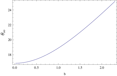


It is easy to obtain that our results reduce to those in the Schwarzschild black hole spacetime as . Moreover, from the Table 2, we also find that as the parameter increases, the minimum impact parameter and the angular position of the relativistic images increase as well, which is contrary to the Reissner-Norström case. The appearance of tells us that the relativistic Einstein ring is much bigger than teh Schwarzschild lensing. The angular separation appears to behave similarly as in the Reissner-Norström case. Also, the relative magnitude stays the same as in Schwarzschild lensing, that is to say, the relative flux of the first image is not affected by phantom scalar fields (dark energy).
From Figure 5, we can see that for the phantom black hole an increase of the parameter causes an increase of both the angular position and the angular separation . This means that the bending angle is bigger in the phantom black hole spacetime. In order to identify the nature of the lensing of these two compact objects, it is necessary to measure the angular separation and the relative magnification in the astronomical observations. Table 2 tells us that the resolution of the extreme angular separation image is arcsecond, which is too small. However, as new technologies are developed the effects of the phantom constant on gravitational lensing may be detected in the future.
Observations of the time delay are given in Table 3. By comparing the results with those in Ref.[30], we can see that both the relativistic Einstein ring (when ) and the time delay become larger with the phantom constant .
| (arcsec) | as) | (min) | as) | (min) | as) | (min) | as) | (min) | as) | (min) |
| 48.60849 | 38.3701 | 50.17959 | 38.4742 | 54.45789 | 39.3316 | 67.78770 | 42.3771 | 73.35538 | 43.5699 | |
| 46.60849 | 38.3702 | 48.17959 | 38.4742 | 52.45789 | 39.3316 | 65.78770 | 42.3771 | 71.35538 | 43.5699 | |
| 28.60848 | 38.3703 | 30.17959 | 38.4742 | 34.45789 | 39.3316 | 47.78770 | 42.3771 | 53.35538 | 43.5699 | |
| 38.3704 | 38.4742 | 42.3771 | 43.5699 | |||||||
| 38.3706 | 38.4742 | 39.5665 | 42.3771 | 43.5699 | ||||||
VI Summary
Modern observations show that the Universe is expanding with an acceleration that is dominated by a peculiar kind of matter (e.g., dark energy) which can be modeled by quintessence or phantom scalar fields. This unknown matter has unusual properties such as negative values of the pressure-to-density ratio. If it exists, then it will inevitably affect the known spacetimes such as black hole physics. Studying strong gravitational lensing can help us probe its existence and properties from astronomical observations. We have investigated strong-field lensing in the phantom black hole spacetime to study the influence of the phantom constant on strong gravitational lensing. The model was applied to the supermassive black hole at the Galactic Center.
Our results show that with an increase of the phantom constant both the minimum impact parameter and the angular position of the relativistic images increase, which contrary to the case of Reissner-Norström black hole lensing with an electric charge . The photon sphere and relative magnitudes stay the same as those of a Schwarzschild black hole and are independent on , which is also contrary to the case where they are weakened by an electric charge. However, the deflect angle and the angular separation appear to have similar behavior as in Reissner-Norström lensing. This may offer a way to distinguish a phantom black hole from a Reissner-Norström one using the astronomical instruments developed in the future.
Our results also show the effects of dark energy in the considered model, such as (i) compressing the usual black hole and more powerfully attracting photons, (ii) making the relativistic Einstein ring larger than the usual black hole, and (iii) not weakening the usual relative magnitudes, which will facilitate observations.
Two days after this paper was published to the arXiv, Ref. [39] appeared online in the same database, containing a partial overlap with our work.
Acknowledgements.
This work was supported by the National Natural Science Foundation of China under No. 11247013, the Hunan Provincial NSFC No. 11JJ3014, the Scientific Research Fund of the Hunan Provincial Education Department No. 11B067, the Foundation for the Author of Hunan Provincial Excellent Doctoral Dissertation No. YB2012B034, and the Aid program for Science and Technology Innovative Research Team in Higher Educational Institutions of Hunan Province.Appendix: Energy density and pressure of phantom fields
With the metric (2), the components for the energy-momentum tensor of phantom fields are
| (32) | |||||
We can rewrite them as a appropriate general expression [38],
| (33) | |||||
so that the spatial part is proportional to the time component with the arbitrary parameter depending on the internal structure of phantom fields. An isotropic averaging over the angles gives
| (34) |
and therefore . After such a treatment, the results are
| (35) | |||||
At last, we obtain the expressions for the pressure and pressure-to-energy density ratio
| (36) | |||||
References
- [1] N. A. Bachall, J. P. Ostriker, S. Perlmutter and P. J. Steinhardt, Science 284, 1481 (1999); S. J. Perlmutter et al, Astrophys. J. 517, 565 (1999); V. Sahni and A. A. Starobinsky, Int. J. Mod. Phys. D 9, 373 (2000).
- [2] K. A. Bronnikov, R. A. Konoplya and A. Zhidenko, Phys. Rev. D. 86, 024028 (2012).
- [3] E. Komatsu, Astrophys. J. Suppl. Ser. 192, 18 (2011).
- [4] M. Sullivan et al., Astrophys. J. 737, 102 (2011).
- [5] R. Gannouji, D. Polarski, A. Ranquet and A. A. Starobinsky, JCAP 0609, 016 (2006); A. Vikman, Phys. Rev. D 71, 023515 (2005); R. R. Caldwell, M. Kamionkowski and N. N. Weinberg, Phys. Rev. Lett.91, 071301 (2003); S. Chattopadhyay and U. Debnath, Braz. J. Phys. 39 86 (2009); Z. Y. Sun and Y. G. Shen, Gen. Rel. Grav. 37, 243 (2005); L. P. Chimento and R. Lazkoz, Phys. Rev. Lett. 91, 211301 (2003).
- [6] E. O. Babichev, V. I. Dokuchaev and Y. N. Eroshenko, Phys. Rev. Lett. 93, 021102 ( 2004); A. V. Frolov, Phys. Rev. D 70 061501 (2004).
- [7] V. Berezin, V. Dokuchaev, Yu. Eroshenko and A. Smirnov, Class. Quantum Grav. 22, 4443 (2005).
- [8] K. A. Bronnikov and J. C. Fabris, Phys. Rev. Lett. 96, 251101 (2006).
- [9] B. McBreen and L. Metcalfe, Nature 330 348 (1987).
- [10] C. C. Dyer and R. C. Roeder, Astrophys. J. Lett. 241 L133 (1980).
- [11] X. Wu, Astron. Astrophys. 214, 43 (1989).
- [12] J. R. Gott, Nature 321, 420 (1986).
- [13] K. Chang and S. Refsdal, Nature 282 561 (1979).
- [14] P. Schneider, J. Ehlers, and E. E. Falco, Gravitational Lenses, Springer-Verlag, Berlin (1992).
- [15] A. F. Zakharov, Gravitational Lenses and Microlenses, Janus-K, Moscow (1997).
- [16] R. D. Blandford and R. Narayan, Annu. Rev. Astron. Astrophys. 30, 311 (1992).
- [17] C. Darwin, Proc. R. Soc. London, 249, 180 (1959).
- [18] K. S. Virbhadra, D. Narasimha and S. M. Chitre, Astron. Astrophys. 337 , 1-8 (1998).
- [19] K. S. Virbhadra and G. F. R. Ellis, Phys. Rev. D 62, 084003 (2000).
- [20] C. M. Claudel, K. S. Virbhadra and G. F. R. Ellis, J. Math. Phys. 42, 818 (2001).
- [21] K. S. Virbhadra and G. F. R. Ellis, Phys. Rev.D 65, 103004 (2002).
- [22] S. Frittelli, T. P. Kling and E. T. Newman, Phys. Rev. D 61, 064021 (2000).
- [23] V. Bozza, Phys. Rev. D 66, 103001 (2002).
- [24] A. Bhadra, Phys. Rev. D 67, 103009 (2003).
- [25] K. Sarkar and A. Bhadra, Class. Quant. Grav. 23, 6101 (2006).
- [26] E. F. Eiroa, G. E. Romero and D. F. Torres, Phys. Rev. D 66, 024010 (2002).
- [27] R. A. Konoplya, Phys. Rev. D 74, 124015 (2006); Phys. Lett. B 644, 219 (2007).
- [28] N. Mukherjee and A. S. Majumdar, astro-ph/0605224 (2006).
- [29] V. Perlick, Phys. Rev. D 69, 064017 (2004).
- [30] K. S. Virbhadra, Phys . Rev. D 79 083004 (2009); K. S. Virbhadra and C. R. Keeton, Phys . Rev. D 77 124014 (2008).
- [31] S. Chen and J. Jing, Phys. Rev. D 80, 024036 (2009).
- [32] A. Y. Bin-Nun, arXiv: 1011.5848 [gr-qc].
- [33] G. N. Gyulchev and I. Z. Stefanov, Phys. Rev. D 87, 063005 (2013).
- [34] V. Bozza, S. Capozziello, G. lovane and G. Scarpetta, Gen. Rel. Grav. 33, 1535 (2001).
- [35] S. Weinberg, Gravitation and Cosmology: Principles and Applications of the General Theory of Relativity (Wiley, New York, 1972).
- [36] D. Richstone et al., Nature 395, A14 (1998).
- [37] F. Eisenhauer et al., Astrophys. J. 628, 246 (2005).
- [38] V. V. Kiselev, Class. Quant. Grav. 20 1187 (2003); S. Chen, B. Wang and R. Su, Phys . Rev. D 77 124011 (2008).
- [39] E. F. Eiroa and C. M. Sendra, arXiv:1308.5959.