跳到论文正文
W Papers独立论文阅读器 arXiv:1308.5000 论文正文 计算阅读时间 · 0%
引用这篇论文根据当前论文元数据生成,正式投稿前建议核对。


License: arXiv.org perpetual non-exclusive license
arXiv:1308.5000v2 [math.OC] 14 Jan 2014

Smoothing and Decomposition for Analysis Sparse Recovery

Zhao Tan    Yonina C. Eldar    Amir Beck    and Arye Nehorai ††thanks: Z. Tan and A. Nehorai are with the Preston M. Green Department of Electrical and Systems Engineering Department, Washington University in St. Louis, St. Louis, MO, 63130 USA. E-mail: {tanz, nehorai}@ese.wustl.edu.††thanks: Y. C. Eldar is with the Department of Electrical Engineering, Technion—Israel Institute of Technology, Haifa 32000, Isreal. E-mail: yonina@ee.technion.ac.il.††thanks: A. Beck is with the Department of Industrial Enigneering and Management, Technion—Israel Institute of Technology, Haifa 32000, Isreal. E-mail: becka@ee.technion.ac.il.††thanks: The work of Z. Tan and A. Nehorai was supported by the AFOSR Grant FA9550-11-1-0210, NSF Grant CCF-1014908, and ONR Grant N000141310050. The work of Y. C. Eldar was supported in part by the Israel Science Foundation under Grant no. 170/10, in part by the Ollendorf Foundation, in part by a Magnet grant Metro450 from the Israel Ministry of Industry and Trade, and in part by the Intel Collaborative Research Institute for Computational Intelligence (ICRI-CI). The work of A. Beck was partially supported by the Israel Science Foundation under grant ISF No.253/12.
Abstract

We consider algorithms and recovery guarantees for the analysis sparse model in which the signal is sparse with respect to a highly coherent frame. We consider the use of a monotone version of the fast iterative shrinkage-thresholding algorithm (MFISTA) to solve the analysis sparse recovery problem. Since the proximal operator in MFISTA does not have a closed-form solution for the analysis model, it cannot be applied directly. Instead, we examine two alternatives based on smoothing and decomposition transformations that relax the original sparse recovery problem, and then implement MFISTA on the relaxed formulation. We refer to these two methods as smoothing-based and decomposition-based MFISTA. We analyze the convergence of both algorithms, and establish that smoothing-based MFISTA converges more rapidly when applied to general nonsmooth optimization problems. We then derive a performance bound on the reconstruction error using these techniques. The bound proves that our methods can recover a signal sparse in a redundant tight frame when the measurement matrix satisfies a properly adapted restricted isometry property. Numerical examples demonstrate the performance of our methods and show that smoothing-based MFISTA converges faster than the decomposition-based alternative in real applications, such as MRI image reconstruction.

Index Terms: 
Analysis model, sparse recovery, fast iterative shrinkage-thresholding algorithm, smoothing and decomposition, convergence analysis, restricted isometry property.

I Introduction

Low-dimensional signal recovery exploits the fact that many natural signals are inherently low dimensional, although they may have high ambient dimension. Prior information about the low-dimensional space can be exploited to aid in recovery of the signal of interest. Sparsity is one of the popular forms of prior information, and is the prior that underlies the growing field of compressive sensing [1]-[4]. Recovery of sparse inputs has found many applications in areas such as imaging, speech, radar signal processing, sub-Nyquist sampling and more. A typical sparse recovery problem has the following linear form:

𝒃=𝑨​𝒙+𝒘,\bm{b}=\bm{A}\bm{x}+\bm{w}, (1)

in which 𝑨∈ℝm×n\bm{A}\in\mathbb{R}^{m\times n} is a measurement matrix, 𝒃∈ℝm\bm{b}\in\mathbb{R}^{m} is the measurement vector, and 𝒘∈ℝm\bm{w}\in\mathbb{R}^{m} represents the noise term. Our goal is to recover the signal 𝒙∈ℝn\bm{x}\in\mathbb{R}^{n}. Normally we have m<nm<n, which indicates that the inverse problem is ill-posed and has infinitely many solutions. To find a unique solution, prior information on 𝒙\bm{x} must be incorporated.

In the synthesis approach to sparse recovery, it is assumed that 𝒙\bm{x} can be expressed as a sparse combination of known dictionary elements, represented as columns of a matrix 𝑫∈ℝn×p\bm{D}\in\mathbb{R}^{n\times p} with p≥np\geq n. That is 𝒙=𝑫​𝜶\bm{x}=\bm{D}\bm{\alpha} with 𝜶\bm{\alpha} sparse, i.e., the number of non-zero elements in 𝜶\bm{\alpha} is far less than the length of 𝜶\bm{\alpha}. The main methods for solving this problem can be classified into two categories. One includes greedy methods, such as iterative hard thresholding [5] and orthogonal matching pursuit [6]. The other is based on relaxation-type methods, such as basis pursuit [7] and LASSO [8]. These methods can stably recover a sparse signal 𝜶\bm{\alpha} when the matrix 𝑨​𝑫\bm{A}\bm{D} satisfies the restricted isometry property (RIP) [9]-[11].

Recently, an alternative approach has became popular, which is known as the analysis method [12], [13]. In this framework, we are given an analysis dictionary 𝑫∗​(𝑫∈ℝn×p)\bm{D}^{*}(\bm{D}\in\mathbb{R}^{n\times p}) under which 𝑫∗​𝒙\bm{D}^{*}\bm{x} is sparse. Assuming, for example, that the ℓ2\ell_{2} norm of the noise 𝒘\bm{w} is bounded by ε\varepsilon, the recovery problem can be formulated as

min𝒙∈ℝn‖𝑫∗​𝒙‖0subject to ​‖𝒃−𝑨​𝒙‖2≤ε.\mathop{\min}_{\bm{x}\in\mathbb{R}^{n}}\|\bm{D}^{*}\bm{x}\|_{0}\quad\text{subject to }\|\bm{b}-\bm{A}\bm{x}\|_{2}\leq\varepsilon. (2)

Since this problem is NP hard, several greedy algorithms have been proposed to approximate it, such as thresholding [14] and subspace pursuit [15].

Alternatively, the nonconvex ℓ0\ell_{0} norm can be approximated by the convex ℓ1\ell_{1} norm leading to the following relaxed problem, referred to as analysis basis pursuit (ABP):

min𝒙∈ℝn‖𝑫∗​𝒙‖1subject to ​‖𝒃−𝑨​𝒙‖2≤ε.\quad\mathop{\min}_{\bm{x}\in\mathbb{R}^{n}}\|\bm{D}^{*}\bm{x}\|_{1}\quad\text{subject to }\|\bm{b}-\bm{A}\bm{x}\|_{2}\leq\varepsilon. (3)

ABP is equivalent to the unconstrained optimization

min𝒙∈ℝn12​‖𝒃−𝑨​𝒙‖22+λ​‖𝑫∗​𝒙‖1,\quad\mathop{\min}_{\bm{x}\in\mathbb{R}^{n}}\frac{1}{2}\|\bm{b}-\bm{A}\bm{x}\|^{2}_{2}+\lambda\|\bm{D}^{*}\bm{x}\|_{1}, (4)

which we call analysis LASSO (ALASSO). The equivalence is in the sense that for any ε>0\varepsilon>0 there exists a λ\lambda for which the optimal solutions of ABP and ALASSO are identical.

Both optimization problems ABP and ALASSO can be solved using interior point methods [16]. However, when the problem dimension grows, these techniques become very slow since they require solutions of linear systems. Another suggested approach is based on alternating direction method of multipliers (ADMM) [17, 18]. The efficiency of this method highly depends on nice structure of the matrices 𝑨\bm{A}. Fast versions of first-order algorithms, such as the fast iterative shrinkage-thresholding algorithm (FISTA) [19], are more favorable in dealing with large dimensional data since they do not require 𝑨\bm{A} to have any structure. The difficulty in directly applying first-order techniques to ABP (3) and ALASSO (4) is the fact that the nonsmooth term ‖𝑫∗​𝒙‖1\|\bm{D}^{*}\bm{x}\|_{1} is inseparable. A generalized iterative soft-thresholding algorithm was proposed in [20] to tackle this difficulty. However, this approach converges relatively slow as we will show in one of our numerical examples. A common alternative is to transform the nondifferentiable problem into a smooth counterpart. In [21], the authors used Nesterov’s smoothing-based method [22] in conjunction with continuation (NESTA) to solve ABP (3), under the assumption that the matrix 𝑨∗​𝑨\bm{A}^{*}\bm{A} is an orthogonal projector. In [23], a smoothed version of ALASSO (4) is solved using a nonlinear conjugate gradient descent algorithm. To avoid imposing conditions on 𝑨\bm{A}, we focus in this paper on the ALASSO formulation (4).

It was shown in [24] that one can apply any fast first-order method that achieves an ε\varepsilon-optimal solution within O⁡(1ε)O(\frac{1}{\sqrt{\varepsilon}}) iterations, to an ε\varepsilon smooth-approximation of the general nonsmooth problem and obtain an algorithm with O⁡(1ε)O(\frac{1}{\varepsilon}) iterations. In this paper, we choose a monotone version of FISTA (MFISTA) [25] as our fast first-order method, whose objective function values are guaranteed to be non-increasing. We apply the smoothing approach together with MFISTA leading to the smoothing-based MFISTA (SFISTA) algorithm. We also propose a decomposition-based MFISTA method (DFISTA) to solve the analysis sparse recovery problem. The decomposition idea is to introduce an auxiliary variable 𝒛\bm{z} in (4) so that MFISTA can be applied in a simple and explicit manner. This decomposition approach can be traced back to [26], and has been widely used for solving total variation problems in the context of image reconstruction [27].

Both smoothing and decomposition based algorithms for nonsmooth optimization problems are very popular in the literature. One of the main goals of this paper is to examine their respective performance. We show that SFISTA requires lower computational complexity to reach a predetermined accuracy. Our results can be applied to a general model, and are not restricted to the analysis sparse recovery problem.

In the context of analysis sparse recovery, we show in Section II-C that both smoothing and decomposition techniques solve the following optimization problem:

min𝒙∈ℝn,𝒛∈ℝp12​‖𝑨​𝒙−𝒃‖22+λ​‖𝒛‖1+12​ρ​‖𝒛−𝑫∗​𝒙‖22,\quad\mathop{\min}_{\bm{x}\in\mathbb{R}^{n},\bm{z}\in\mathbb{R}^{p}}\frac{1}{2}\bm{\|}\bm{A}\bm{x}-\bm{b}\|_{2}^{2}+\lambda\|\bm{z}\|_{1}+\frac{1}{2}\rho\|\bm{z}-\bm{D}^{*}\bm{x}\|_{2}^{2},\\ (5)

which we refer to as relaxed ALASSO (RALASSO). Another contribution of this paper is in proving recovery guarantees for RALASSO (5). With the introduction of the restricted isometry property adapted to 𝑫\bm{D} (D-RIP) [12], previous work [12] [28] studied recovery guarantees based on ABP (3) and ALASSO (4). Here we combine the techniques in [9] and [28], and obtain a performance bound on RALASSO (5). We show that when σ2​s<0.1907\sigma_{2s}<0.1907 and ‖𝑫∗​𝑨∗​𝒘‖∞≤λ2\|\bm{D}^{*}\bm{A}^{*}\bm{w}\|_{\infty}\leq\frac{\lambda}{2}, the solution 𝒙^ρ\hat{\bm{x}}_{\rho} of RALASSO (5) satisfies

‖𝒙^ρ−𝒙‖2≤C0​s​λ+C1​‖𝑫∗​𝒙−(𝑫∗​𝒙)s‖1s+C2​λ​ps​ρ,\|\hat{\bm{x}}_{\rho}-\bm{x}\|_{2}\leq C_{0}\sqrt{s}\lambda+C_{1}\frac{\|\bm{D}^{*}\bm{x}-(\bm{D}^{*}\bm{x})_{s}\|_{1}}{\sqrt{s}}+C_{2}\frac{\lambda p}{\sqrt{s}\rho}, (6)

where pp is the number of rows in 𝑫∗\bm{D}^{*}, C0,C1,C2C_{0},C_{1},C_{2} are constants, and we use (𝒙)s(\bm{x})_{s} to denote the vector consisting of the largest ss entries of |𝒙||\bm{x}|. As a special case, choosing ρ→∞\rho\to\infty extends the bound in (6) and obtains the reconstruction bound for ALASSO (4) as long as σ2​s<0.1907\sigma_{2s}<0.1907, which improves upon the results of [28].

The paper is organized as follows. In Section II, we introduce some mathematical preliminaries, and present SFISTA and DFISTA for solving RALASSO (5). We analyze the convergence behavior of these two algorithms in Section III, and show that SFISTA converges faster than DFISTA for a general model. Performance guarantees on RALASSO (5) are developed in Section IV. Finally, in Section V we test our techniques on numerical experiments to demonstrate the effectiveness of our algorithms in solving the analysis recovery problem. We show that SFISTA performs favorably in comparison with DFISTA. A continuation method is also introduced to further accelerate the convergence speed.

Throughout the paper, we use capital italic bold letters to represent matrices and lowercase italic bold letters to represent vectors. For a given matrix 𝑫\bm{D}, 𝑫∗\bm{D}^{*} denotes the conjugate matrix. We denote by 𝑫𝒯∗\bm{D}^{*}_{\mathcal{T}} the matrix that maintains the rows in 𝑫∗\bm{D}^{*} with indices in set 𝒯\mathcal{T}, while setting all other rows to zero. Given a vector 𝒙\bm{x}, ‖𝒙‖1,‖𝒙‖2\|\bm{x}\|_{1},\|\bm{x}\|_{2} are the ℓ1,ℓ2\ell_{1},\ell_{2} norms respectively, ‖𝒙‖0\|\bm{x}\|_{0} counts the number of nonzero components which will be referred to as the ℓ0\ell_{0} norm although it is not a norm, and ‖𝒙‖∞\|\bm{x}\|_{\infty} denotes the maximum absolute value of the elements in 𝒙\bm{x}. We use 𝒙⁡[i]\bm{x}[i] to represent the iith element of 𝒙\bm{x}. For a matrix 𝑨\bm{A}, ‖𝑨‖2\|\bm{A}\|_{2} is the induced spectral norm, and ‖𝑨‖p,q=max‖𝑨​𝒙‖p‖𝒙‖q.\|\bm{A}\|_{p,q}=\mathop{\max}\frac{\|\bm{A}\bm{x}\|_{p}}{\|\bm{x}\|_{q}}. Finally, Re​⟨𝒂,𝒃⟩=⟨𝒂,𝒃⟩+⟨𝒃,𝒂⟩2.\mathrm{Re}\langle\bm{a},\bm{b}\rangle=\frac{\langle\bm{a},\bm{b}\rangle+\langle\bm{b},\bm{a}\rangle}{2}. We use argmin{f(𝒙):𝒙=𝒛,𝒚}\mathrm{argmin}\{f(\bm{x}):\bm{x}=\bm{z},\bm{y}\} to denote 𝒛\bm{z} or 𝒚\bm{y}, whichever yields a smaller function value of f⁡(𝒙)f(\bm{x}).

II Smoothing and Decomposition for Analysis Sparse Recovery

In this section we present the smoothing-based and decomposition-based methods for solving ALASSO (4). To do so, we first recall in Subsection II-A some results related to proximal gradient methods that will be essential to our presentation and analysis.

II-A The Proximal Gradient Method

We begin this section with the definition of Moreau’s proximal (or “prox”) operator [29], which is the key step in defining the proximal gradient method.

Given a closed proper convex function h:ℝn→ℝ∪{∞}h:\mathbb{R}^{n}\rightarrow\mathcal{\mathbb{R}}\cup\{\infty\}, the proximal operator of hh is defined by

proxh​(𝒙)=arg⁡min𝒖∈ℝn​{h⁡(𝒖)+12​‖𝒖−𝒙‖22}.\mathrm{prox}_{h}(\bm{x})=\underset{\bm{u}\in\mathbb{R}^{n}}{\arg\min}\left\{h(\bm{u})+\frac{1}{2}\|\bm{u}-\bm{x}\|^{2}_{2}\right\}. (7)

The proximal operator can be computed efficiently in many important instances. For example, it can be easily obtained when hh is an lpl_{p} norm (OPENp∈[1,∞))p\in[1,\infty)), or an indicator of “simple” closed convex sets such as the box, unit-simplex and the ball. More examples of proximal operators as well as a wealth of properties can be found, for example, in [30] [31].

The proximal operator can be used in order to compute smooth approximations of convex functions. Specifically, let hh be a closed, proper, convex function, and let μ>0\mu>0 be a given parameter. Define

hμ​(𝒙)=min𝒖∈ℝn⁡{h⁡(𝒖)+12​μ​‖𝒖−𝒙‖22}.h_{\mu}(\bm{x})=\min_{\bm{u}\in\mathbb{R}^{n}}\left\{h(\bm{u})+\frac{1}{2\mu}\|\bm{u}-\bm{x}\|_{2}^{2}\right\}. (8)

It is easy to see that

hμ​(𝒙)=h⁡(proxμ​h​(𝒙))+12​μ​‖𝒙−proxμ​h​(𝒙)‖22.h_{\mu}(\bm{x})=h({\rm prox}_{\mu h}(\bm{x}))+\frac{1}{2\mu}\|\bm{x}-{\rm prox}_{\mu h}(\bm{x})\|_{2}^{2}. (9)

The function hμh_{\mu} is called the Moreau envelope of hh and has the following important properties (see [29] for further details):

  • •

    hμ​(𝒙)≤h​(𝒙)h_{\mu}(\bm{x})\leq h(\bm{x}).

  • •

    hμh_{\mu} is continuously differentiable and its gradient is Lipschitz continuous with constant 1/μ1/\mu.

  • •

    The gradient of hμh_{\mu} is given by

    ∇hμ​(𝒙)=1μ​(𝒙−proxμ​h​(𝒙)).\nabla h_{\mu}(\bm{x})=\frac{1}{\mu}(\bm{x}-{\rm prox}_{\mu h}(\bm{x})). (10)

One important usage of the proximal operator is in the proximal gradient method that is aimed at solving the following composite problem:

min𝒙∈ℝn⁡{F⁡(𝒙)+G⁡(𝒙)}.\min_{\bm{x}\in\mathbb{R}^{n}}\{F(\bm{x})+G(\bm{x})\}. (11)

Here F:ℝn→ℝF:{\mathbb{R}}^{n}\rightarrow\mathbb{R} is a continuously differentiable convex function with a continuous gradient that has Lipschitz constant L∇FL_{\nabla F}:

‖∇F​(𝒙)−∇F​(𝒚)‖2≤L∇F​‖𝒙−𝒚‖2, for all ​𝒙,𝒚∈ℝn,\|\nabla F(\bm{x})-\nabla F(\bm{y})\|_{2}\leq L_{\nabla F}\|\bm{x}-\bm{y}\|_{2},\quad\mbox{ for all }\bm{x},\bm{y}\in{\mathbb{R}}^{n},

and G:ℝn→ℝ∪{∞}G:{\mathbb{R}}^{n}\rightarrow{\mathbb{R}}\cup\{\infty\} is an extended-valued, proper, closed and convex function. The proximal gradient method for solving (11) takes the following form (see [19, 32]):

Proximal Gradient Method For Solving (11)
Input: An upper bound L≥L∇FL\geq L_{\nabla F}.
Step 0. Take 𝒙0∈ℝn.\bm{x}_{0}\in\mathbb{R}^{n}.
Step k. (k≥1k\geq 1)
     Compute 𝒙k=prox1L​G(𝒙k−1−1L∇F(𝒙k−1)).\bm{x}_{k}={\rm prox}_{\frac{1}{L}G}\left(\bm{x}_{k-1}-\frac{1}{L}\nabla F(\bm{x}_{k-1})\right).

The main disadvantage of the proximal gradient method is that it suffers from a relatively slow O⁡(1/k)O(1/k) rate of convergence of the function values. An accelerated version is the fast proximal gradient method, also known in the literature as fast iterative shrinkage thresholding algorithm (FISTA) [19, 32]. When G≡0G\equiv 0, the problem is smooth, and FISTA coincides with Nesterov’s optimal gradient method [33]. In this paper we implement a monotone version of FISTA (MFISTA) [25], which guarantees that the objective function value is non-increasing along the iterations.

Monotone FISTA Method (MFISTA) For Solving (11)
Input: An upper bound L≥L∇FL\geq L_{\nabla F}.
Step 0. Take 𝒚1=𝒙0,t1=1.\bm{y}_{1}=\bm{x}_{0},t_{1}=1.
Step k. (k≥1k\geq 1) Compute
     𝒛k=prox1L​G(𝒚k−1L∇F(𝒚k)).\bm{z}_{k}={\rm prox}_{\frac{1}{L}G}\left(\bm{y}_{k}-\frac{1}{L}\nabla F(\bm{y}_{k})\right).
     tk+1=1+1+4​tk22t_{k+1}=\frac{1+\sqrt{1+4t^{2}_{k}}}{2}.
     𝒙k=argmin{F(𝒙)+G(𝒙):𝒙=𝒛k,𝒙k−1}\bm{x}_{k}=\mathrm{argmin}\{F(\bm{x})+G(\bm{x}):\bm{x}=\bm{z}_{k},\bm{x}_{k-1}\}.
     𝒚k+1=𝒙k+tktk+1​(𝒛k−𝒙k)+tk−1tk+1​(𝒙k−𝒙k−1)\bm{y}_{k+1}=\bm{x}_{k}+\frac{t_{k}}{t_{k+1}}(\bm{z}_{k}-\bm{x}_{k})+\frac{t_{k}-1}{t_{k+1}}(\bm{x}_{k}-\bm{x}_{k-1}).

The rate of convergence of the sequence generated by MFISTA is O⁡(1/k2)O(1/k^{2}).

Theorem II.1.

[25] Let {𝐱k}k≥0\{\bm{x}_{k}\}_{k\geq 0} be the sequence generated by MFISTA, and let 𝐱^\hat{\bm{x}} be an optimal solution of (11). Then

F⁡(𝒙k)+G⁡(𝒙k)−F⁡(𝒙^)−G⁡(𝒙^)≤2​L∇F​‖𝒙0−𝒙^‖22(k+1)2.F(\bm{x}_{k})+G(\bm{x}_{k})-F(\hat{\bm{x}})-G(\hat{\bm{x}})\leq\frac{2L_{\nabla F}\|\bm{x}_{0}-\hat{\bm{x}}\|_{2}^{2}}{(k+1)^{2}}. (12)

II-B The General Nonsmooth Model

The general optimization model we consider in this paper is

min𝒙∈ℝn{H(𝒙)=f(𝒙)+g(𝑫∗𝒙)},\quad\mathop{\min}_{\bm{x}\in\mathbb{R}^{n}}\{H(\bm{x})=f(\bm{x})+g(\bm{D}^{*}\bm{x})\}, (13)

where f:ℝn→ℝf:\mathbb{R}^{n}\rightarrow\mathbb{R} is a continuously differentiable convex function with a Lipschitz continuous gradient L∇fL_{\nabla f}. The function g:ℝp→ℝ∪{∞}g:\mathbb{R}^{p}\rightarrow\mathbb{R}\cup\{\infty\} is a closed, proper convex function which is not necessarily smooth, and 𝑫∗∈ℝp×n\bm{D}^{*}\in\mathbb{R}^{p\times n} is a given matrix. In addition, we assume that gg is Lipschitz continuous with parameter LgL_{g}:

|g⁡(𝒛)−g⁡(𝒗)|≤Lg​‖𝒛−𝒗‖2 for all ​𝒛,𝒗∈ℝp.|g(\bm{z})-g(\bm{v})|\leq L_{g}\|\bm{z}-\bm{v}\|_{2}\quad\mbox{ for all }\bm{z},\bm{v}\in\mathbb{R}^{p}.

This is equivalent to saying that the subgradients of gg over ℝp\mathbb{R}^{p} are bounded by LgL_{g}:

‖g′​(𝒛)‖2≤Lg​ for any ​𝒙∈ℝn​ and ​g′​(𝒛)∈∂g⁡(𝒛).\|g^{\prime}(\bm{z})\|_{2}\leq L_{g}\text{ for any }\bm{x}\in\mathbb{R}^{n}\text{ and }g^{\prime}(\bm{z})\in\partial g(\bm{z}).

An additional assumption we make throughout is that the proximal operator of α​g​(𝒛)\alpha g(\bm{z}) for any α>0\alpha>0 can be easily computed.

Directly applying MFISTA to (13) requires computing the proximal operator of g⁡(𝑫∗​𝒙)g(\bm{D}^{*}\bm{x}). Despite the fact that we assume that it is easy to compute the proximal operator of g⁡(𝒛)g(\bm{z}), it is in general difficult to compute that of α​g​(𝑫∗​𝒙)\alpha g(\bm{D}^{*}\bm{x}). Therefore we need to transform the problem before utilizing MFISTA, in order to avoid this computation.

When considering ALASSO, f⁡(𝒙)=12​‖𝑨​𝒙−𝒃‖22f(\bm{x})=\frac{1}{2}\|\bm{A}\bm{x}-\bm{b}\|_{2}^{2} and g⁡(𝑫∗​𝒙)=λ​‖𝑫∗​𝒙‖1g(\bm{D}^{*}\bm{x})=\lambda\|\bm{D}^{*}\bm{x}\|_{1}. The Lipschitz constants are given by L∇f=‖𝑨‖22L_{\nabla f}=\|\bm{A}\|_{2}^{2} and Lg=λ​pL_{g}=\lambda\sqrt{p}. The proximal operator of α​g​(𝒛)=α​λ​‖𝒛‖1\alpha g(\bm{z})=\alpha\lambda\|\bm{z}\|_{1} can be computed as

proxα​g​(𝒛)=Γλ​α​(𝒛)=[|𝒛|−λ​α]+​sgn​(𝒛),\displaystyle\mathrm{prox}_{\alpha g}(\bm{z})=\Gamma_{\lambda\alpha}(\bm{z})=[|\bm{z}|-\lambda\alpha]_{+}\mathrm{sgn}(\bm{z}), (14)

where for brevity, we denote the soft shrinkage operator by Γλ​α​(𝒛).\Gamma_{\lambda\alpha}(\bm{z}). Here [𝒛]+[\bm{z}]_{+} denotes the vector whose components are given by the maximum between ziz_{i} and 00. Note, however, that there is no explicit expression for the proximal operator of g⁡(𝑫∗​𝒙)=λ​‖𝑫∗​𝒙‖1g(\bm{D}^{*}\bm{x})=\lambda\|\bm{D}^{*}\bm{x}\|_{1}, i.e., there is no closed form solution to

arg⁡min𝒖∈ℝn​{α​λ​‖𝑫∗​𝒖‖1+12​‖𝒖−𝒙‖22}.\underset{\bm{u}\in\mathbb{R}^{n}}{\arg\min}\left\{\alpha\lambda\|\bm{D}^{*}\bm{u}\|_{1}+\frac{1}{2}\|\bm{u}-\bm{x}\|^{2}_{2}\right\}. (15)

In the next subsection, we introduce two popular approaches for transforming the problem (13): smoothing and decomposition. We will show in Sections II-D and II-E that both transformations lead to algorithms which only require computation of the proximal operator of g⁡(𝒛)g(\bm{z}), and not that of g⁡(𝑫∗​𝒙)g(\bm{D}^{*}\bm{x}).

II-C The Smoothing and Decomposition Transformations

The first approach to transform (13) is the smoothing method in which the nonsmooth function g⁡(𝒛)g(\bm{z}) is replaced by its Moreau envelope gμ​(𝒛)g_{\mu}(\bm{z}), which can be seen as a smooth approximation. By letting 𝒛=𝑫∗​𝒙\bm{z}=\bm{D}^{*}\bm{x} , the smoothed problem becomes

min𝒙∈ℝn{Hμ(𝒙)=f(𝒙)+gμ(𝑫∗𝒙)},\quad\mathop{\min}_{\bm{x}\in\mathbb{R}^{n}}\{H_{\mu}(\bm{x})=f(\bm{x})+g_{\mu}(\bm{D}^{*}\bm{x})\}, (16)

to which MFISTA can be applied since it only requires evaluating the proximal operator of g⁡(𝒛)g(\bm{z}). From the general properties of the Moreau envelope, and from the fact that the norms of the subgradients of gg are bounded above by LgL_{g}, we can deduce that there exists some β1\beta_{1}, β2>0\beta_{2}>0 such that β1+β2=Lg\beta_{1}+\beta_{2}=L_{g} and g⁡(𝒛)−β1​μ≤gμ​(𝒛)≤g⁡(𝒛)+β2​μ​ for all ​𝒛∈ℝpg(\bm{z})-\beta_{1}\mu\leq g_{\mu}(\bm{z})\leq g(\bm{z})+\beta_{2}\mu\mbox{ for all }\bm{z}\in\mathbb{R}^{p} (see [24, 22]). This shows that a smaller μ\mu leads to a finer approximation.

The second approach for transforming the problem is the decomposition method in which we consider:

min𝒙∈ℝn,𝒛∈ℝp{Gρ(𝒙,𝒛)=f(𝒙)+g(𝒛)+ρ2∥𝒛−𝑫∗𝒙∥22}.\mathop{\min}_{\bm{x}\in\mathbb{R}^{n},\bm{z}\in\mathbb{R}^{p}}\left\{G_{\rho}(\bm{x},\bm{z})=f(\bm{x})+g(\bm{z})+\frac{\rho}{2}\|\bm{z}-\bm{D}^{*}\bm{x}\|^{2}_{2}\right\}. (17)

With ρ→∞\rho\to\infty, this problem is equivalent to the following constrained formulation of the original problem (13):

min⁡{f⁡(𝒙)+g⁡(𝒛)}\displaystyle\min\{f(\bm{x})+g(\bm{z})\}
s.t.𝒛=𝑫∗​𝒙,𝒙∈ℝn,𝒛∈ℝp.\displaystyle\mbox{s.t.}\quad\bm{z}=\bm{D}^{*}\bm{x},\quad\bm{x}\in\mathbb{R}^{n},\bm{z}\in\mathbb{R}^{p}.\ (18)

Evidently, there is a close relationship between the approximate models (16) and (17). Indeed, fixing 𝒙\bm{x} and minimizing the objective function of (17) with respect to 𝒛\bm{z} we obtain

min𝒙∈ℝn,𝒛∈ℝp⁡{f⁡(𝒙)+g⁡(𝒛)+ρ2​‖𝒛−𝑫∗​𝒙‖22}\displaystyle\min_{\bm{x}\in\mathbb{R}^{n},\bm{z}\in\mathbb{R}^{p}}\left\{f(\bm{x})+g(\bm{z})+\frac{\rho}{2}\|\bm{z}-\bm{D}^{*}\bm{x}\|_{2}^{2}\right\}
=min𝒙∈ℝn⁡{f⁡(𝒙)+g1ρ​(𝑫∗​𝒙)}.\displaystyle=\min_{\bm{x}\in\mathbb{R}^{n}}\left\{f(\bm{x})+g_{\frac{1}{\rho}}(\bm{D}^{*}\bm{x})\right\}. (19)

Therefore, the two models are equivalent in the sense that their optimal solution set (limited to 𝒙\bm{x}) is the same when μ=1ρ\mu=\frac{1}{\rho}. For analysis sparse recovery, both transformations lead to RALASSO (5). However, as we shall see, the resulting smoothing-based and decomposition-based algorithms and their analysis are very different.

II-D The Smoothing-Based Method

Since (16) is a smooth problem we can apply an optimal first-order method such as MFISTA with F=Hμ=f⁡(𝒙)+gμ​(𝑫∗​𝒙)F=H_{\mu}=f(\bm{x})+g_{\mu}(\bm{D}^{*}\bm{x}) and G≡0G\equiv 0 in equation (11). The Lipschitz constant of HμH_{\mu} is given by L∇f+‖𝑫‖22μL_{\nabla f}+\frac{\|\bm{D}\|^{2}_{2}}{\mu}, and according to (10) the gradient of ∇gμ​(𝑫∗​𝒙)\nabla g_{\mu}(\bm{D}^{*}\bm{x}) is equal to 1μ​𝑫​(𝑫∗​𝒙−proxμ​g​(𝑫∗​𝒙))\frac{1}{\mu}\bm{D}(\bm{D}^{*}\bm{x}-{\rm prox}_{\mu g}(\bm{D}^{*}\bm{x})). The expression proxμ​g​(𝑫∗​𝒙)\mathrm{prox}_{\mu g}(\bm{D}^{*}\bm{x}) is calculated by first computing proxμ​g​(𝒛)\mathrm{prox}_{\mu g}(\bm{z}), and then letting 𝒛=𝑫∗​𝒙\bm{z}=\bm{D}^{*}\bm{x}.

Returning to the analysis sparse recovery problem, after smoothing we obtain

min𝒙∈ℝn{Hμ(𝒙)=12∥𝑨𝒙−𝒃∥22+gμ(𝑫∗𝒙)},\min_{\bm{x}\in\mathbb{R}^{n}}\left\{H_{\mu}(\bm{x})=\frac{1}{2}\bm{\|}\bm{A}\bm{x}-\bm{b}\|_{2}^{2}+g_{\mu}(\bm{D}^{*}\bm{x})\right\}, (20)

where

gμ​(𝑫∗​𝒙)=\displaystyle g_{\mu}(\bm{D}^{*}\bm{x})= min𝒖{λ​‖𝒖‖1+12​μ​‖𝒖−𝑫∗​𝒙‖22}\displaystyle\mathop{\min}_{\bm{u}}\left\{\lambda\|\bm{u}\|_{1}+\frac{1}{2\mu}\|\bm{u}-\bm{D}^{*}\bm{x}\|_{2}^{2}\right\}
=\displaystyle= ∑i=1pλ​ℋλ​μ​((𝑫∗​𝒙)​[i]).\displaystyle\sum_{i=1}^{p}\lambda\mathcal{H}_{\lambda\mu}((\bm{D}^{*}\bm{x})[i]).

The function ℋα​(x)\mathcal{H}_{\alpha}(x) with parameter α>0\alpha>0 is the so-called Huber function [34], and is given by

ℋα​(x)={12​α​x2if ​|x|<α|x|−α2otherwise.\mathcal{H}_{\alpha}(x)=\left\{\begin{array}[]{ll}\frac{1}{2\alpha}x^{2}&\text{if }|x|<\alpha\\ |x|-\frac{\alpha}{2}&\text{otherwise}.\\ \end{array}\right. (21)

From (14), the gradient of gμ​(𝑫∗​𝒙)g_{\mu}(\bm{D}^{*}\bm{x}) is equal to

∇gμ​(𝑫∗​𝒙)=1μ​𝑫​(𝑫∗​𝒙−Γλ​μ​(𝑫∗​𝒙)).\nabla g_{\mu}(\bm{D}^{*}\bm{x})=\frac{1}{\mu}\bm{D}(\bm{D}^{*}\bm{x}-\Gamma_{\lambda\mu}(\bm{D}^{*}\bm{x})). (22)

Applying MFISTA to (20), results in the SFISTA algorithm, summarized in Algorithm 1.

Algorithm1: Smoothing-based MFISTA (SFISTA)
Input: An upper bound L≥‖𝑨‖22+‖𝑫‖22μL\geq\|\bm{A}\|_{2}^{2}+\frac{\|\bm{D}\|^{2}_{2}}{\mu}.
Step 0. Take 𝒚1=𝒙0,t1=1.\bm{y}_{1}=\bm{x}_{0},t_{1}=1.
Step k. (k≥1k\geq 1) Compute
∇f​(𝒚k)=𝑨∗​(𝑨​𝒚k−𝒃)\nabla f(\bm{y}_{k})=\bm{A}^{*}(\bm{A}\bm{y}_{k}-\bm{b}).
∇gμ​(𝑫∗​𝒙k−1)=1μ​𝑫​(𝑫∗​𝒙k−1−Γλ​μ​(𝑫∗​𝒙k−1))\nabla g_{\mu}(\bm{D}^{*}\bm{x}_{k-1})=\frac{1}{\mu}\bm{D}(\bm{D}^{*}\bm{x}_{k-1}-\Gamma_{\lambda\mu}(\bm{D}^{*}\bm{x}_{k-1})).
𝒛k=𝒚k−1L​(∇f​(𝒚k)+∇gμ​(𝑫∗​𝒙k−1))\bm{z}_{k}=\bm{y}_{k}-\frac{1}{L}(\nabla f(\bm{y}_{k})+\nabla g_{\mu}(\bm{D}^{*}\bm{x}_{k-1})).
tk+1=1+1+4​tk22t_{k+1}=\frac{1+\sqrt{1+4t^{2}_{k}}}{2}.
𝒙k=argmin{Hμ(𝒙):𝒙=𝒛k,𝒙k−1}\bm{x}_{k}=\mathrm{argmin}\{H_{\mu}(\bm{x}):\bm{x}=\bm{z}_{k},\bm{x}_{k-1}\}.
𝒚k+1=𝒙k+tktk+1​(𝒛k−𝒙k)+tk−1tk+1​(𝒙k−𝒙k−1)\bm{y}_{k+1}=\bm{x}_{k}+\frac{t_{k}}{t_{k+1}}(\bm{z}_{k}-\bm{x}_{k})+\frac{t_{k}-1}{t_{k+1}}(\bm{x}_{k}-\bm{x}_{k-1}).

II-E The Decomposition-Based Method

We can also employ MFISTA on the decomposition model

min𝒙∈ℝn,𝒛∈ℝp{Gρ(𝒙,𝒛)=Fρ(𝒙,𝒛)+G(𝒙,𝒛)},\min_{\bm{x}\in\mathbb{R}^{n},\bm{z}\in\mathbb{R}^{p}}\{G_{\rho}(\bm{x},\bm{z})=F_{\rho}(\bm{x},\bm{z})+G(\bm{x},\bm{z})\}, (23)

where we take the smooth part as Fρ​(𝒙,𝒛)=f⁡(𝒙)+ρ2​‖𝒛−𝑫∗​𝒙‖22F_{\rho}(\bm{x},\bm{z})=f(\bm{x})+\frac{\rho}{2}\|\bm{z}-\bm{D}^{*}\bm{x}\|^{2}_{2} and the nonsmooth part as G⁡(𝒙,𝒛)=g⁡(𝒛)G(\bm{x},\bm{z})=g(\bm{z}). In order to apply MFISTA to (17), we need to compute the proximal operator of α​G\alpha G for a given constant α>0\alpha>0, which is given by

proxα​G​(𝒙,𝒛)=(𝒙proxα​g​(𝒛)).\displaystyle\mathrm{prox}_{\alpha G}(\bm{x},\bm{z})=\begin{pmatrix}\bm{x}\\ {\rm prox}_{\alpha g}(\bm{z})\\ \end{pmatrix}. (24)

In RALASSO (5), G⁡(𝒙,𝒛)=λ​‖𝒛‖1G(\bm{x},\bm{z})=\lambda\|\bm{z}\|_{1} and Fρ​(𝒙,𝒛)=12​‖𝑨​𝒙−𝒃‖22+12​ρ​‖𝒛−𝑫∗​𝒙‖22F_{\rho}(\bm{x},\bm{z})=\frac{1}{2}\bm{\|}\bm{A}\bm{x}-\bm{b}\|_{2}^{2}+\frac{1}{2}\rho\|\bm{z}-\bm{D}^{*}\bm{x}\|_{2}^{2}. Therefore,

proxα​G​(𝒙,𝒛)=(𝒙Γλ​α​(𝒛)).\mathrm{prox}_{\alpha G}(\bm{x},\bm{z})=\begin{pmatrix}\bm{x}\\ \Gamma_{\lambda\alpha}(\bm{z})\\ \end{pmatrix}. (25)

The Lipschitz constant of ∇F\nabla F is equal to (‖𝑨‖22+ρ⁡(1+‖𝑫‖22))(\|\bm{A}\|_{2}^{2}+\rho(1+\|\bm{D}\|_{2}^{2})). By applying MFISTA directly, we have the DFISTA algorithm, stated in Algorithm 2.

Algorithm 2:Decomposition-based MFISTA (DFISTA)
Input: An upper bound L≥(‖𝑨‖22+ρ⁡(1+‖𝑫‖22))L\geq(\|\bm{A}\|_{2}^{2}+\rho(1+\|\bm{D}\|_{2}^{2})).
Step 0. Take 𝒖1=𝒙0,𝒗1=𝒛0,t1=1.\bm{u}_{1}=\bm{x}_{0},\bm{v}_{1}=\bm{z}_{0},t_{1}=1.
Step k. (k≥1k\geq 1) Compute
∇𝒙Fρ​(𝒖k,𝒗k)=𝑨∗​(𝑨​𝒖k−𝒃)+ρ​𝑫​(𝑫∗​𝒖k−𝒗k)\nabla_{\bm{x}}F_{\rho}(\bm{u}_{k},\bm{v}_{k})=\bm{A}^{*}(\bm{A}\bm{u}_{k}-\bm{b})+\rho\bm{D}(\bm{D}^{*}\bm{u}_{k}-\bm{v}_{k}).
OPEN∇𝒛Fρ​(𝒖k,𝒗k))=ρ⁡(𝒗k−𝑫∗​𝒖k)\nabla_{\bm{z}}F_{\rho}(\bm{u}_{k},\bm{v}_{k}))=\rho(\bm{v}_{k}-\bm{D}^{*}\bm{u}_{k}).
𝒑k=𝒖k−1L​∇𝒙Fρ​(𝒖k,𝒗k)\bm{p}_{k}=\bm{u}_{k}-\frac{1}{L}\nabla_{\bm{x}}F_{\rho}(\bm{u}_{k},\bm{v}_{k}).
𝒒k=ΓλL​(𝒗k−1L​∇𝒛Fρ​(𝒖k,𝒗k))\bm{q}_{k}=\Gamma_{\frac{\lambda}{L}}(\bm{v}_{k}-\frac{1}{L}\nabla_{\bm{z}}F_{\rho}(\bm{u}_{k},\bm{v}_{k})).
tk+1=1+1+4​tk22t_{k+1}=\frac{1+\sqrt{1+4t^{2}_{k}}}{2}.
(𝒙k,𝒛k)(\bm{x}_{k},\bm{z}_{k})
=argmin{Gρ(𝒙,𝒛):(𝒙,𝒛)=(𝒑k,𝒒k),(𝒙k−1,𝒛k−1)}=\mathrm{argmin}\{G_{\rho}(\bm{x},\bm{z}):(\bm{x},\bm{z})=(\bm{p}_{k},\bm{q}_{k}),(\bm{x}_{k-1},\bm{z}_{k-1})\}.
𝒖k+1=𝒙k+tktk+1​(𝒑k−𝒙k)+tk−1tk+1​(𝒙k−𝒙k−1)\bm{u}_{k+1}=\bm{x}_{k}+\frac{t_{k}}{t_{k+1}}(\bm{p}_{k}-\bm{x}_{k})+\frac{t_{k}-1}{t_{k+1}}(\bm{x}_{k}-\bm{x}_{k-1}).
𝒗k+1=𝒛k+tktk+1​(𝒒k−𝒛k)+tk−1tk+1​(𝒛k−𝒛k−1)\bm{v}_{k+1}=\bm{z}_{k}+\frac{t_{k}}{t_{k+1}}(\bm{q}_{k}-\bm{z}_{k})+\frac{t_{k}-1}{t_{k+1}}(\bm{z}_{k}-\bm{z}_{k-1}).

III Convergence Analysis

In this section we analyze the convergence behavior of both the smoothing-based and decomposition-based methods. Convergence of smoothing algorithms has been treated in [22, 24]. In order to make the paper self contained, we quote the main results here. We then analyze the convergence of the decomposition approach. Both methods require the same type of operations at each iteration: the computation of the gradient of the smooth function ff, and of the proximal operator corresponding to α​g\alpha g, which means that they have the same computational cost per iteration. However, we show that smoothing converges faster than decomposition based methods. Specifically, the smoothing-based algorithm is guaranteed to generate an ε\varepsilon-optimal solution within O⁡(1/ε)O(1/\varepsilon) iterations, whereas the decomposition-based approach requires O⁡(1/ε1.5)O(1/\varepsilon^{1.5}) iterations. We prove the results by analyzing SFISTA and DFISTA for the general problem (13), however, the same analysis can be easily extended to other optimal first-order methods, such as the one described in [22].

III-A Convergence of the Smoothing-Based Method

For SFISTA the sequence {𝒙k}\{\bm{x}_{k}\} satisfies the following relationship [25]:

Hμ​(𝒙k)−Hμ​(𝒙^μ)≤2​(L∇f+‖𝑫‖22μ)​Λ1(k+1)2,H_{\mu}(\bm{x}_{k})-H_{\mu}(\hat{\bm{x}}_{\mu})\leq\frac{2\left(L_{\nabla f}+\frac{\|\bm{D}\|^{2}_{2}}{\mu}\right)\Lambda_{1}}{(k+1)^{2}}, (26)

where Λ1\Lambda_{1} is an upper bound on the expression ‖𝒙^μ−𝒙0‖2\|\hat{\bm{x}}_{\mu}-\bm{x}_{0}\|_{2} with 𝒙^μ\hat{\bm{x}}_{\mu} being an arbitrary optimal solution of the smoothed problem (16), and 𝒙0\bm{x}_{0} is the initial point of the algorithm. Of course, this rate of convergence is problematic since we are more interested in bounding the expression H⁡(𝒙k)−H^H(\bm{x}_{k})-\hat{H} rather than the expression Hμ​(𝒙k)−Hμ​(𝒙^μ)H_{\mu}(\bm{x}_{k})-H_{\mu}(\hat{\bm{x}}_{\mu}), which is in terms of the smoothed problem. Here, H^\hat{H} stands for the optimal value for original nonsmooth problem (13). For that, we can use the following result from [24].

Theorem III.1.

[24] Let {𝒙k\bm{x}_{k}} be the sequence generated by applying MFISTA to the problem (16). Let 𝐱0\bm{x}_{0} be the initial point and let 𝐱^\hat{\bm{x}} denote the optimal solution of (13). An ε\varepsilon-optimal solution of (13), i.e. |H⁡(𝐱k)−H⁡(𝐱^)|≤ε|H(\bm{x}_{k})-H(\hat{\bm{x}})|\leq\varepsilon, is obtained in the smoothing-based method using MFISTA after at most

K=2​‖𝑫‖2​Lg​Λ1​1ε+L∇f​Λ1​1εK=2\|\bm{D}\|_{2}\sqrt{L_{g}\Lambda_{1}}\frac{1}{\varepsilon}+\sqrt{L_{\nabla f}\Lambda_{1}}\frac{1}{\sqrt{\varepsilon}} (27)

iterations with μ\mu chosen as

μ=‖𝑫‖22Lg​ε‖𝑫‖22​Lg+‖𝑫‖22​Lg+L∇f​ε,\mu=\sqrt{\frac{\|\bm{D}\|_{2}^{2}}{L_{g}}}\frac{\varepsilon}{\sqrt{\|\bm{D}\|_{2}^{2}L_{g}}+\sqrt{\|\bm{D}\|_{2}^{2}L_{g}+L_{\nabla f}\varepsilon}}, (28)

in which LgL_{g} and L∇fL_{\nabla f} are the Lipschitz constants of gg and the gradient function of ff in (13), and Λ1=‖𝐱0−𝐱^μ‖2\Lambda_{1}=\|\bm{x}_{0}-\hat{\bm{x}}_{\mu}\|_{2}. We use 𝐱^μ\hat{\bm{x}}_{\mu} to denote the optimal solution of problem (16).

Remarks: For analysis sparse recovery using SFISTA, Lg=λ​p12L_{g}=\lambda p^{\frac{1}{2}} and L∇f=‖𝑨‖22L_{\nabla f}=\|\bm{A}\|_{2}^{2}, which can be plugged into the expressions in the theorem.

III-B Convergence of the Decomposition-Based Method

A key property of the decomposition model (17) is that its minimal value is bounded above by the optimal value H^\hat{H} in the original problem (13).

Lemma III.1.

Let G^ρ\hat{G}_{\rho} be the optimal value of problem (17) and H^\hat{H} be the optimal value of problem (13). Then G^ρ≤H^\hat{G}_{\rho}\leq\hat{H}.

Proof: The proof follows from adding the constraint 𝒛=𝑫∗​𝒙\bm{z}=\bm{D}^{*}\bm{x} to the optimization:

G^ρ=\displaystyle\hat{G}_{\rho}= min𝒙∈ℝn,𝒛∈ℝp{f⁡(𝒙)+g⁡(𝒛)+ρ2​‖𝒛−𝑫∗​𝒙‖22}\displaystyle\mathop{\min}_{\bm{x}\in\mathbb{R}^{n},\bm{z}\in\mathbb{R}^{p}}\left\{f(\bm{x})+g(\bm{z})+\frac{\rho}{2}\|\bm{z}-\bm{D}^{*}\bm{x}\|^{2}_{2}\right\}
≤\displaystyle\leq min𝒙∈ℝn,𝒛∈ℝp,𝒛=𝑫∗​𝒙{f⁡(𝒙)+g⁡(𝒛)+ρ2​‖𝒛−𝑫∗​𝒙‖22}\displaystyle\mathop{\min}_{\bm{x}\in\mathbb{R}^{n},\bm{z}\in\mathbb{R}^{p},\bm{z}=\bm{D}^{*}\bm{x}}\left\{f(\bm{x})+g(\bm{z})+\frac{\rho}{2}\|\bm{z}-\bm{D}^{*}\bm{x}\|^{2}_{2}\right\}
=\displaystyle= min𝒙∈ℝn{f⁡(𝒙)+g⁡(𝑫∗​𝒙)},\displaystyle\mathop{\min}_{\bm{x}\in\mathbb{R}^{n}}\left\{f(\bm{x})+g(\bm{D}^{*}\bm{x})\right\}, (29)

which is equal to H^\hat{H}.

The next theorem is our main convergence result establishing that an ε\varepsilon-optimal solution can be reached after O⁡(1/ε1.5)O(1/\varepsilon^{1.5}) iterations. By assuming that the functions ff and gg are nonnegative, which is not an unusual assumption, we have the following theorem.

Theorem III.2.

Let {𝐱k,𝐳k}\{\bm{x}_{k},\bm{z}_{k}\} be the sequences generated by applying MFISTA to (17) with both ff and gg both being nonnegative functions. The initial point is taken as (𝐱0,𝐳0)(\bm{x}_{0},\bm{z}_{0}) with 𝐳0=𝐃∗​𝐱0\bm{z}_{0}=\bm{D}^{*}\bm{x}_{0}. Let 𝐱^\hat{\bm{x}} denote the optimal solution of the original problem (13). An ε\varepsilon-optimal solution of problem (13), i.e. |H⁡(𝐱k)−H⁡(𝐱^)|≤ε|H(\bm{x}_{k})-H(\hat{\bm{x}})|\leq\varepsilon, is obtained using the decomposition-based method after at most

K=max⁡{16​(1+‖𝑫‖2​Λ2​H​(𝒙0))​Lgε1.5,2​L∇f​Λ2ε}K=\mathrm{max}\left\{\frac{16\sqrt{(1+\|\bm{D}\|^{2}\Lambda_{2}H(\bm{x}_{0}))}L_{g}}{\varepsilon^{1.5}},\frac{2\sqrt{L_{\nabla f}\Lambda_{2}}}{\sqrt{\varepsilon}}\right\} (30)

iterations of MFISTA with ρ\rho chosen as

ρ=(Lg​2​H​(𝒙0)​K22​(1+‖𝑫‖2)​Λ2)2/3.\rho=\left(\frac{L_{g}\sqrt{2H(\bm{x}_{0})}K^{2}}{2(1+\|\bm{D}\|^{2})\Lambda_{2}}\right)^{2/3}. (31)

Here LgL_{g} and L∇fL_{\nabla f} are the Lipschitz constants for gg and the gradient function of ff in (13), and Λ2=‖𝐱0−𝐱^ρ‖22+‖𝐳0−𝐳^ρ‖22\Lambda_{2}=\|\bm{x}_{0}-\hat{\bm{x}}_{\rho}\|^{2}_{2}+\|\bm{z}_{0}-\hat{\bm{z}}_{\rho}\|^{2}_{2}. We use 𝐱^ρ,𝐳^ρ\hat{\bm{x}}_{\rho},\hat{\bm{z}}_{\rho} to denote the optimal solutions to (17).

Proof: Since the monotone version of FISTA is applied we have

f⁡(𝒙k)+g⁡(𝒛k)+ρ2​‖𝒛k−𝑫∗​𝒙k‖22\displaystyle f(\bm{x}_{k})+g(\bm{z}_{k})+\frac{\rho}{2}\|\bm{z}_{k}-\bm{D}^{*}\bm{x}_{k}\|_{2}^{2}
=\displaystyle= Gρ​(𝒙k,𝒛k)≤Gρ​(𝒙0,𝒛0)=f⁡(𝒙0)+g⁡(𝑫∗​𝒙0)=H⁡(𝒙0).\displaystyle G_{\rho}(\bm{x}_{k},\bm{z}_{k})\leq G_{\rho}(\bm{x}_{0},\bm{z}_{0})=f(\bm{x}_{0})+g(\bm{D}^{*}\bm{x}_{0})=H(\bm{x}_{0}). (32)

With the assumption that ff and gg are nonnegative, it follows that

ρ2​‖𝒛k−𝑫∗​𝒙k‖22≤H⁡(𝒙0),\frac{\rho}{2}\|\bm{z}_{k}-\bm{D}^{*}\bm{x}_{k}\|^{2}_{2}\leq H(\bm{x}_{0}),

and therefore

‖𝒛k−𝑫∗​𝒙k‖2≤2​H​(𝒙0)ρ.\|\bm{z}_{k}-\bm{D}^{*}\bm{x}_{k}\|_{2}\leq\sqrt{\frac{2H(\bm{x}_{0})}{\rho}}. (33)

The gradient of f⁡(𝒙)+ρ2​‖𝒛−𝑫∗​𝒙‖22f(\bm{x})+\frac{\rho}{2}\|\bm{z}-\bm{D}^{*}\bm{x}\|_{2}^{2}, is Lipschitz continuous with parameter (L∇f+ρ⁡(1+‖𝑫‖22))(L_{\nabla f}+\rho(1+\|\bm{D}\|_{2}^{2})). According to [25], by applying MFISTA, we obtain a sequence {(𝒙k,𝒛k)}\{(\bm{x}_{k},\bm{z}_{k})\} satisfying

Gρ​(𝒙k,𝒛k)−G^ρ≤2​(L∇f+ρ⁡(1+‖𝑫‖22))​Λ2k2.G_{\rho}(\bm{x}_{k},\bm{z}_{k})-\hat{G}_{\rho}\leq\frac{2(L_{\nabla f}+\rho(1+\|\bm{D}\|^{2}_{2}))\Lambda_{2}}{k^{2}}.

Using lemma III.1 and the notation

A=2​L∇f​Λ2,B=2​(1+‖𝑫‖22)​Λ2,\displaystyle A=2L_{\nabla f}\Lambda_{2},B=2(1+\|\bm{D}\|^{2}_{2})\Lambda_{2},

we have

Gρ​(𝒙k,𝒛k)−H^≤A+ρ​Bk2.G_{\rho}(\bm{x}_{k},\bm{z}_{k})-\hat{H}\leq\frac{A+\rho B}{k^{2}}. (34)

We therefore conclude that

H⁡(𝒙k)=\displaystyle H(\bm{x}_{k})= f⁡(𝒙k)+g⁡(𝑫∗​𝒙k)\displaystyle f(\bm{x}_{k})+g(\bm{D}^{*}\bm{x}_{k})
=\displaystyle= f⁡(𝒙k)+g⁡(𝒛k)+g⁡(𝑫∗​𝒙k)−g⁡(𝒛k)\displaystyle f(\bm{x}_{k})+g(\bm{z}_{k})+g(\bm{D}^{*}\bm{x}_{k})-g(\bm{z}_{k})
≤\displaystyle\leq Gρ​(𝒙k,𝒛k)+Lg​‖𝒛k−𝑫∗​𝒙k‖2\displaystyle G_{\rho}(\bm{x}_{k},\bm{z}_{k})+L_{g}\|\bm{z}_{k}-\bm{D}^{*}\bm{x}_{k}\|_{2}
≤\displaystyle\leq H^+A+ρ​Bk2+Lg​‖𝒛k−𝑫∗​𝒙k‖2\displaystyle\hat{H}+\frac{A+\rho B}{k^{2}}+L_{g}\|\bm{z}_{k}-\bm{D}^{*}\bm{x}_{k}\|_{2}
≤\displaystyle\leq H^+A+ρ​Bk2+Lg​2​H​(𝒙0)ρ.\displaystyle\hat{H}+\frac{A+\rho B}{k^{2}}+L_{g}\sqrt{\frac{2H(\bm{x}_{0})}{\rho}}.

The first inequality follows from the Lipschitz condition for the function gg, the second inequality is obtained from (34), and the last inequality is a result of (33).

We now seek the “best” ρ\rho that minimizes the upper bound, or equivalently, minimizes the term

A+ρ​Bk2+Lg​2​H​(𝒙0)ρ=Ak2+C​ρ+Dρ,\frac{A+\rho B}{k^{2}}+L_{g}\sqrt{\frac{2H(\bm{x}_{0})}{\rho}}=\frac{A}{k^{2}}+C\rho+\frac{D}{\sqrt{\rho}}, (35)

where C=Bk2C=\frac{B}{k^{2}} and D=Lg​2​H​(𝒙0)D=L_{g}\sqrt{2H(\bm{x}_{0})}. Setting the derivative to zero, the optimal value of ρ\rho is ρ=(D2​C)2/3\rho=\left(\frac{D}{2C}\right)^{2/3}, and

H⁡(𝒙k)≤H^+Ak2+2​C1/3​D2/3.H(\bm{x}_{k})\leq\hat{H}+\frac{A}{k^{2}}+2C^{1/3}D^{2/3}. (36)

Therefore, to obtain an ε\varepsilon-optimal solution, it is enough that

Ak2≤ε2,2​B1/3​D2/3k2/3≤ε2,\frac{A}{k^{2}}\leq\frac{\varepsilon}{2},\quad\frac{2B^{1/3}D^{2/3}}{k^{2/3}}\leq\frac{\varepsilon}{2}, (37)

or

k≥\displaystyle k\geq max​{43/2​B1/2​Dε1.5,2​Aε}\displaystyle\mathrm{max}\left\{\frac{4^{3/2}B^{1/2}D}{\varepsilon^{1.5}},\frac{\sqrt{2A}}{\sqrt{\varepsilon}}\right\}
=\displaystyle= max​{16​(1+‖𝑫‖2​Λ2​H​(𝒙0))​Lgε1.5,2​L∇f​Λ2ε},\displaystyle\mathrm{max}\left\{\frac{16\sqrt{(1+\|\bm{D}\|^{2}\Lambda_{2}H(\bm{x}_{0}))}L_{g}}{\varepsilon^{1.5}},\frac{2\sqrt{L_{\nabla f}\Lambda_{2}}}{\sqrt{\varepsilon}}\right\}, (38)

completing the proof.

Remarks:
1. As in SFISTA, when treating the analysis sparse recovery problem, Lg=λ​p12L_{g}=\lambda p^{\frac{1}{2}} and L∇f=‖𝑨‖22L_{\nabla f}=\|\bm{A}\|_{2}^{2}, which again can be plugged into the expressions in the theorem.
2. MFISTA is applied in SFISTA and DFISTA to guarantee a mathematical rigorous proof, i.e. the existence of equation (32). In real application, FISTA without monotone operations can also be applied to yield corresponding smoothing and decomposition based algorithms.

Comparing the results of smoothing-based and decomposition-based methods, we immediately conclude that the smoothing-based method is preferable. First, it requires only O⁡(1/ε)O(1/\varepsilon) iterations to obtain an ε\varepsilon-optimal solution whereas the decomposition approach necessitates O⁡(1/ε3/2)O(1/\varepsilon^{3/2}) iterations. Note that both bounds are better than the bound O⁡(1/ε2)O(1/\varepsilon^{2}) corresponding to general sub-gradient schemes for nonsmooth optimization. Second, the bound in the smoothing approach depends on Lg\sqrt{L_{g}}, and not on LgL_{g}, as when using decomposition methods. This is important since, for example, when g⁡(𝒛)=‖𝒛‖1g(\bm{z})=\|\bm{z}\|_{1}, we have Lg=p12L_{g}=p^{\frac{1}{2}}. In the smoothing approach the dependency on pp is of the form p14p^{\frac{1}{4}} and not p12p^{\frac{1}{2}}, as when using the decomposition algorithm.

IV Performance Bounds

We now turn to analyze the recovery performance of analysis LASSO when smoothing and decomposition are applied. As we have seen, both transformations lead to the same RALASSO problem in (5). Our main result in this section shows that the reconstruction obtained by solving RALASSO is stable when 𝑫∗​𝒙\bm{D}^{*}\bm{x} has rapidly decreasing coefficients and the noise in the model (1) is small enough. Our performance bound also depends on the choice of parameter ρ\rho in the objective function. Before stating the main theorems, we first introduce a definition and some useful lemmas, whose proofs are detailed in the Appendix.

To ensure stable recovery, we require that the matrix 𝑨{\bm{A}} satisfies the D-RIP:

Definition IV.1.

(D-RIP) [12]. The measurement matrix 𝐀\bm{A} obeys the restricted isometry property adapted to 𝐃\bm{D} with constant σs\sigma_{s} if

(1−σs)​‖𝒗‖22≤‖𝑨​𝒗‖22≤(1+σs)​‖𝒗‖22(1-\sigma_{s})\|\bm{v}\|_{2}^{2}\leq\|\bm{A}\bm{v}\|_{2}^{2}\leq(1+\sigma_{s})\|\bm{v}\|_{2}^{2} (39)

holds for all 𝐯∈Σs={𝐲:𝐲=𝐃​𝐱​ and ​‖𝐱‖0≤s}\bm{v}\in\Sigma_{s}=\{\bm{y}:\bm{y}=\bm{D}\bm{x}\text{ and }\|\bm{x}\|_{0}\leq s\}. In other words, Σs\Sigma_{s} is the union of subspaces spanned by all subsets of ss columns of 𝐃\bm{D}.

The following lemma provides a useful inequality for matrices satisfying D-RIP.

Lemma IV.1.

Let 𝐀\bm{A} satisfy the D-RIP with parameter σ2​s\sigma_{2s}, and assume that 𝐮,𝐯∈Σs\bm{u},\bm{v}\in\Sigma_{s}. Then,

Re⁡⟨𝑨​𝒖,𝑨​𝒗⟩≥−σ2​s​‖𝒖‖2​‖𝒗‖2+Re⁡⟨𝒖,𝒗⟩.\mathrm{Re}\langle\bm{A}\bm{u},\bm{A}\bm{v}\rangle\geq-\sigma_{2s}\|\bm{u}\|_{2}\|\bm{v}\|_{2}+\mathrm{Re}\langle\bm{u},\bm{v}\rangle. (40)

In the following, 𝒙^ρ\hat{\bm{x}}_{\rho} denotes the optimal solution of RALASSO (5) and 𝒙\bm{x} is the original signal in the linear model (1); we also use 𝒉\bm{h} to represent the reconstruction error 𝒉=𝒙^ρ−𝒙\bm{h}=\hat{\bm{x}}_{\rho}-\bm{x}. Let 𝒯\mathcal{T} be the indices of coefficients with ss largest magnitudes in the vector 𝑫∗​𝒙\bm{D}^{*}\bm{x}, and denote the complement of 𝒯\mathcal{T} by 𝒯c\mathcal{T}^{c}. Setting 𝒯0=𝒯\mathcal{T}_{0}=\mathcal{T}, we decompose 𝒯0c\mathcal{T}_{0}^{c} into sets of size ss where 𝒯1\mathcal{T}_{1} denotes the locations of the ss largest coefficients in 𝑫𝒯c∗​𝒙\bm{D}_{\mathcal{T}^{c}}^{*}\bm{x}, 𝒯2\mathcal{T}_{2} denote the next ss largest coefficients and so on. Finally, we let 𝒯01=𝒯0∪𝒯1\mathcal{T}_{01}=\mathcal{T}_{0}\cup\mathcal{T}_{1}.

Using the result of Lemma IV.1 and the inequality ‖𝑫𝒯0∗​𝒉‖2+‖𝑫𝒯1∗​𝒉‖2≤2​‖𝑫𝒯01∗​𝒉‖2\|\bm{D}^{*}_{\mathcal{T}_{0}}\bm{h}\|_{2}+\|\bm{D}^{*}_{\mathcal{T}_{1}}\bm{h}\|_{2}\leq\sqrt{2}\|\bm{D}^{*}_{\mathcal{T}_{01}}\bm{h}\|_{2} since 𝒯0\mathcal{T}_{0} and 𝒯1\mathcal{T}_{1} are disjoint, we have the following lemma.

Lemma IV.2.

(D-RIP property) Let 𝐡=𝐱^ρ−𝐱\bm{h}=\hat{\bm{x}}_{\rho}-\bm{x} be the reconstruction error in RALASSO (5). We assume that 𝐀\bm{A} satisfies the D-RIP with parameter σ2​s\sigma_{2s} and 𝐃\bm{D} is a tight frame. Then,

Re⁡⟨𝑨​𝒉,𝑨​𝑫​𝑫𝒯01∗​𝒉⟩\displaystyle\mathrm{Re}\langle\bm{A}\bm{h},\bm{A}\bm{D}\bm{D}^{*}_{\mathcal{T}_{01}}\bm{h}\rangle
≥\displaystyle\geq (1−σ2​s)​‖𝑫𝒯01∗​𝒉‖22−2​s−12​σ2​s​‖𝑫𝒯01∗​𝒉‖2​‖𝑫𝒯c∗​𝒉‖1.\displaystyle(1-\sigma_{2s})\|\bm{D}^{*}_{\mathcal{T}_{01}}\bm{h}\|^{2}_{2}-\sqrt{2}s^{-\frac{1}{2}}\sigma_{2s}\|\bm{D}^{*}_{\mathcal{T}_{01}}\bm{h}\|_{2}\|\bm{D}^{*}_{\mathcal{T}^{c}}\bm{h}\|_{1}. (41)

Finally, the lemmas below show that the reconstruction error 𝒉\bm{h} and ‖𝑫𝒯c∗​𝒉‖1\|\bm{D}^{*}_{\mathcal{T}^{c}}\bm{h}\|_{1} can not be very large.

Lemma IV.3.

(Optimality condition) The optimal solution 𝐱^ρ\hat{\bm{x}}_{\rho} for RALASSO (5) satisfies

‖𝑫∗​𝑨∗​𝑨​𝒉‖∞≤(12+‖𝑫∗​𝑫‖1,1)​λ.\displaystyle\|\bm{D}^{*}\bm{A}^{*}\bm{A}\bm{h}\|_{\infty}\leq\left(\frac{1}{2}+\|\bm{D}^{*}\bm{D}\|_{1,1}\right)\lambda. (42)
Lemma IV.4.

(Cone constraint) The optimal solution 𝐱^ρ\hat{\bm{x}}_{\rho} for RALASSO (5) satisfies the following cone constraint,

‖𝑫𝒯c∗​𝒉‖1≤λρ​p+3​‖𝑫𝒯∗​𝒉‖1+4​‖𝑫𝒯c∗​𝒙‖1.\|\bm{D}^{*}_{\mathcal{T}^{c}}\bm{h}\|_{1}\leq\frac{\lambda}{\rho}p+3\|\bm{D}^{*}_{\mathcal{T}}\bm{h}\|_{1}+4\|\bm{D}^{*}_{\mathcal{T}^{c}}\bm{x}\|_{1}. (43)

We are now ready to state our main result.

Theorem IV.1.

Let 𝐀\bm{A} be an m×nm\times n measurement matrix, 𝐃\bm{D} an arbitrary n×pn\times p tight frame, and let 𝐀\bm{A} satisfy the D-RIP with σ2​s<0.1907\sigma_{2s}<0.1907. Consider the measurement 𝐛=𝐀​𝐱+𝐰\bm{b}=\bm{A}\bm{x}+\bm{w}, where 𝐰\bm{w} is noise that satisfies ‖𝐃∗​𝐀∗​𝐰‖∞≤λ2\|\bm{D}^{*}\bm{A}^{*}\bm{w}\|_{\infty}\leq\frac{\lambda}{2}. Then the solution 𝐱^ρ\hat{\bm{x}}_{\rho} to RALASSO (5) satisfies

‖𝒙^ρ−𝒙‖2≤C0​s​λ+C1​‖𝑫∗​𝒙−(𝑫∗​𝒙)s‖1s+C2​λ​ps​ρ,\|\hat{\bm{x}}_{\rho}-\bm{x}\|_{2}\leq C_{0}\sqrt{s}\lambda+C_{1}\frac{\|\bm{D}^{*}\bm{x}-(\bm{D}^{*}\bm{x})_{s}\|_{1}}{\sqrt{s}}+C_{2}\frac{\lambda p}{\sqrt{s}\rho}, (44)

for the decomposition transformation and

‖𝒙^ρ−𝒙‖2≤C0​s​λ+C1​‖𝑫∗​𝒙−(𝑫∗​𝒙)s‖1s+C2​λ​μ​ps,\|\hat{\bm{x}}_{\rho}-\bm{x}\|_{2}\leq C_{0}\sqrt{s}\lambda+C_{1}\frac{\|\bm{D}^{*}\bm{x}-(\bm{D}^{*}\bm{x})_{s}\|_{1}}{\sqrt{s}}+C_{2}\frac{\lambda\mu p}{\sqrt{s}}, (45)

for the smoothing transformation. Here (𝐃∗​𝐱)s(\bm{D}^{*}\bm{x})_{s} is the vector consisting of the largest ss entries of 𝐃∗​𝐱\bm{D}^{*}\bm{x} in magnitude, C1C_{1} and C2C_{2} are constants depending on σ2​s\sigma_{2s}, and C0C_{0} depends on σ2​s\sigma_{2s} and ‖𝐃∗​𝐃‖1,1\|\bm{D}^{*}\bm{D}\|_{1,1}.

Proof: The proof follows mainly from the ideas in [9], [28], and proceeds in two steps. First, we try to show that 𝑫∗​𝒉\bm{D}^{*}\bm{h} inside 𝒯01\mathcal{T}_{01} is bounded by the terms of 𝑫∗​𝒉\bm{D}^{*}\bm{h} outside the set 𝒯\mathcal{T}. Then we show that 𝑫𝒯c∗​𝒉\bm{D}^{*}_{\mathcal{T}^{c}}\bm{h} is essentially small.

From Lemma IV.2,

Re⁡⟨𝑨​𝒉,𝑨​𝑫​𝑫𝒯01∗​𝒉⟩\displaystyle\mathrm{Re}\langle\bm{A}\bm{h},\bm{A}\bm{D}\bm{D}^{*}_{\mathcal{T}_{01}}\bm{h}\rangle
≥\displaystyle\geq (1−σ2​s)​‖𝑫𝒯01∗​𝒉‖22−2​s−12​σ2​s​‖𝑫𝒯01∗​𝒉‖2​‖𝑫𝒯c∗​𝒉‖1.\displaystyle(1-\sigma_{2s})\|\bm{D}^{*}_{\mathcal{T}_{01}}\bm{h}\|^{2}_{2}-\sqrt{2}s^{-\frac{1}{2}}\sigma_{2s}\|\bm{D}^{*}_{\mathcal{T}_{01}}\bm{h}\|_{2}\|\bm{D}^{*}_{\mathcal{T}^{c}}\bm{h}\|_{1}. (46)

Using the fact that Re⁡⟨𝒙,𝒚⟩≤|⟨𝒙,𝒚⟩|≤‖𝒙‖1​‖𝒚‖∞\mathrm{Re}\langle\bm{x},\bm{y}\rangle\leq|\langle\bm{x},\bm{y}\rangle|\leq\|\bm{x}\|_{1}\|\bm{y}\|_{\infty}, we obtain that

Re⁡⟨𝑨​𝒉,𝑨​𝑫​𝑫𝒯01∗​𝒉⟩=\displaystyle\mathrm{Re}\langle\bm{A}\bm{h},\bm{A}\bm{D}\bm{D}^{*}_{\mathcal{T}_{01}}\bm{h}\rangle= Re⁡⟨𝑫∗​𝑨∗​𝑨​𝒉,𝑫𝒯01∗​𝒉⟩\displaystyle\mathrm{Re}\langle\bm{D}^{*}\bm{A}^{*}\bm{A}\bm{h},\bm{D}^{*}_{\mathcal{T}_{01}}\bm{h}\rangle
≤\displaystyle\leq ‖𝑫∗​𝑨∗​𝑨​𝒉‖∞​‖𝑫𝒯01∗​𝒉‖1\displaystyle\|\bm{D}^{*}\bm{A}^{*}\bm{A}\bm{h}\|_{\infty}\|\bm{D}^{*}_{\mathcal{T}_{01}}\bm{h}\|_{1}
≤\displaystyle\leq 2​s​c0​λ​‖𝑫𝒯01∗​𝒉‖2,\displaystyle\sqrt{2s}c_{0}\lambda\|\bm{D}^{*}_{\mathcal{T}_{01}}\bm{h}\|_{2}, (47)

with c0=12+‖𝑫∗​𝑫‖1,1c_{0}=\frac{1}{2}+\|\bm{D}^{*}\bm{D}\|_{1,1}. The second inequality is a result of Lemma IV.3 and the fact that ‖𝑫𝒯01∗​𝒉‖1≤2​s​‖𝑫𝒯01∗​𝒉‖2\|\bm{D}^{*}_{\mathcal{T}_{01}}\bm{h}\|_{1}\leq\sqrt{2s}\|\bm{D}^{*}_{\mathcal{T}_{01}}\bm{h}\|_{2}, in which 2​s2s is the number of nonzero terms in 𝑫𝒯01∗​𝒉\bm{D}^{*}_{\mathcal{T}_{01}}\bm{h}. Combining (46) and (47), we get

‖𝑫𝒯01∗​𝒉‖2≤2​s​λ​c0+2​s−12​σ2​s​‖𝑫𝒯c∗​𝒉‖11−σ2​s.\|\bm{D}^{*}_{\mathcal{T}_{01}}\bm{h}\|_{2}\leq\frac{\sqrt{2s}\lambda c_{0}+\sqrt{2}s^{-\frac{1}{2}}\sigma_{2s}\|\bm{D}^{*}_{\mathcal{T}^{c}}\bm{h}\|_{1}}{1-\sigma_{2s}}. (48)

Then the second step bounds ‖𝑫𝒯c∗​𝒉‖1\|\bm{D}^{*}_{\mathcal{T}^{c}}\bm{h}\|_{1}. From (48),

‖𝑫𝒯∗​𝒉‖1≤\displaystyle\|\bm{D}^{*}_{\mathcal{T}}\bm{h}\|_{1}\leq s​‖𝑫𝒯∗​𝒉‖2≤s​‖𝑫𝒯01∗​𝒉‖2\displaystyle\sqrt{s}\|\bm{D}^{*}_{\mathcal{T}}\bm{h}\|_{2}\leq\sqrt{s}\|\bm{D}^{*}_{\mathcal{T}_{01}}\bm{h}\|_{2}
≤\displaystyle\leq 2​λ​s​c0+2​σs​‖𝑫𝒯c∗​𝒉‖11−σ2​s.\displaystyle\frac{\sqrt{2}\lambda sc_{0}+\sqrt{2}\sigma_{s}\|\bm{D}^{*}_{\mathcal{T}^{c}}\bm{h}\|_{1}}{1-\sigma_{2s}}. (49)

Finally, using Lemma IV.4 and (49),

‖𝑫𝒯c∗​𝒉‖1≤λρ​p+3​2​λ​s​c0+3​2​σ2​s​‖𝑫𝒯c∗​𝒉‖11−σ2​s+4​‖𝑫𝒯c∗​𝒙‖1.\|\bm{D}^{*}_{\mathcal{T}^{c}}\bm{h}\|_{1}\leq\frac{\lambda}{\rho}p+\frac{3\sqrt{2}\lambda sc_{0}+3\sqrt{2}\sigma_{2s}\|\bm{D}^{*}_{\mathcal{T}^{c}}\bm{h}\|_{1}}{1-\sigma_{2s}}+4\|\bm{D}^{*}_{\mathcal{T}^{c}}\bm{x}\|_{1}. (50)

Since σ2​s<0.1907\sigma_{2s}<0.1907, we have 1−(1+3​2)​σ2​s>01-(1+3\sqrt{2})\sigma_{2s}>0. Rearranging terms, the above inequality becomes

‖𝑫𝒯c∗​𝒉‖1\displaystyle\|\bm{D}^{*}_{\mathcal{T}^{c}}\bm{h}\|_{1}
≤\displaystyle\leq 1−σ2​s1−(1+3​2)​σ2​s​λρ​p+3​2​λ​s​c0+4​(1−σ2​s)​‖𝑫𝒯c∗​𝒙‖11−(1+3​2)​σ2​s.\displaystyle\frac{1-\sigma_{2s}}{1-(1+3\sqrt{2})\sigma_{2s}}\frac{\lambda}{\rho}p+\frac{3\sqrt{2}\lambda sc_{0}+4(1-\sigma_{2s})\|\bm{D}^{*}_{\mathcal{T}^{c}}\bm{x}\|_{1}}{1-(1+3\sqrt{2})\sigma_{2s}}. (51)

We now derive the bound on the reconstruction error. Using the results of (48) and (51), we get

‖𝒉‖2=\displaystyle\|\bm{h}\|_{2}= ‖𝑫∗​𝒉‖2≤‖𝑫𝒯01∗​𝒉‖2+∑j≥2‖𝑫𝒯j∗​𝒉‖2\displaystyle\|\bm{D}^{*}\bm{h}\|_{2}\leq\|\bm{D}^{*}_{\mathcal{T}_{01}}\bm{h}\|_{2}+\sum_{j\geq 2}\|\bm{D}^{*}_{\mathcal{T}_{j}}\bm{h}\|_{2}
≤\displaystyle\leq 2​s​λ​c0+2​s−12​σ2​s​‖𝑫𝒯c∗​𝒉‖11−σ2​s+s−12​‖𝑫𝒯c∗​𝒉‖1\displaystyle\frac{\sqrt{2s}\lambda c_{0}+\sqrt{2}s^{-\frac{1}{2}}\sigma_{2s}\|\bm{D}^{*}_{\mathcal{T}^{c}}\bm{h}\|_{1}}{1-\sigma_{2s}}+s^{-\frac{1}{2}}\|\bm{D}^{*}_{\mathcal{T}^{c}}\bm{h}\|_{1}
=\displaystyle= c0​λ​2​s1−σ2​s+((2−1)​σ2​s+1)​s−12​‖𝑫𝒯c∗​𝒉‖11−σ2​s\displaystyle\frac{c_{0}\lambda\sqrt{2s}}{1-\sigma_{2s}}+\frac{((\sqrt{2}-1)\sigma_{2s}+1)s^{-\frac{1}{2}}\|\bm{D}^{*}_{\mathcal{T}^{c}}\bm{h}\|_{1}}{1-\sigma_{2s}}
≤\displaystyle\leq C0​s​λ+C1​‖𝑫∗​𝒙−(𝑫∗​𝒙)s‖1s+C2​λ​ps​ρ.\displaystyle C_{0}\sqrt{s}\lambda+C_{1}\frac{\|\bm{D}^{*}\bm{x}-(\bm{D}^{*}\bm{x})_{s}\|_{1}}{\sqrt{s}}+C_{2}\frac{\lambda p}{\sqrt{s}\rho}. (52)

The first equality follows from the assumption that 𝑫\bm{D} is a tight frame so that 𝑫​𝑫∗=𝑰\bm{D}\bm{D}^{*}=\bm{I}. The first inequality is the result of the triangle inequality. The second inequality follows from (48) and the fact that ∑j≥2‖𝑫𝒯j∗​𝒉‖2≤s−12​‖𝑫𝒯c∗​𝒉‖1\sum_{j\geq 2}\|\bm{D}^{*}_{\mathcal{T}_{j}}\bm{h}\|_{2}\leq s^{-\frac{1}{2}}\|\bm{D}^{*}_{\mathcal{T}^{c}}\bm{h}\|_{1}, which is proved in equation (58) in the Appendix. The constants in the final result are given by

C0=\displaystyle C_{0}= 4​2​c01−(1+3​2)​σ2​s,\displaystyle\frac{4\sqrt{2}c_{0}}{1-(1+3\sqrt{2})\sigma_{2s}},
C1=\displaystyle C_{1}= 4​((2−1)​σ2​s+1)1−(1+3​2)​σ2​s,\displaystyle\frac{4((\sqrt{2}-1)\sigma_{2s}+1)}{1-(1+3\sqrt{2})\sigma_{2s}},
C2=\displaystyle C_{2}= (2−1)​σ2​s+11−(1+3​2)​σ2​s.\displaystyle\frac{(\sqrt{2}-1)\sigma_{2s}+1}{1-(1+3\sqrt{2})\sigma_{2s}}.\quad

To obtain the error bound for the smoothing transformation we replace ρ\rho with 1/μ1/\mu in the result. □\square

Choosing ρ→∞\rho\rightarrow\infty in RALASSO (5) leads to the ALASSO problem for which 𝒛=𝑫∗​𝒙\bm{z}=\bm{D}^{*}\bm{x}. We then have the following result.

Theorem IV.2.

Let 𝐀\bm{A} be an m×nm\times n measurement matrix, 𝐃\bm{D} an arbitrary n×pn\times p tight frame, and let 𝐀\bm{A} satisfy the D-RIP with σ2​s<0.1907\sigma_{2s}<0.1907. Consider the measurement 𝐛=𝐀​𝐱+𝐰\bm{b}=\bm{A}\bm{x}+\bm{w}, where 𝐰\bm{w} is noise that satisfies ‖𝐃∗​𝐀∗​𝐰‖∞≤λ2\|\bm{D}^{*}\bm{A}^{*}\bm{w}\|_{\infty}\leq\frac{\lambda}{2}. Then the solution 𝐱^\hat{\bm{x}} to ALASSO (4) satisfies

‖𝒙^−𝒙‖2≤C0​s​λ+C1​‖𝑫∗​𝒙−(𝑫∗​𝒙)s‖1s,\|\hat{\bm{x}}-\bm{x}\|_{2}\leq C_{0}\sqrt{s}\lambda+C_{1}\frac{\|\bm{D}^{*}\bm{x}-(\bm{D}^{*}\bm{x})_{s}\|_{1}}{\sqrt{s}}, (53)

where (𝐃∗​𝐱)s(\bm{D}^{*}\bm{x})_{s} is the vector consisting of the largest ss entries of 𝐃∗​𝐱\bm{D}^{*}\bm{x} in magnitude, C1C_{1} is a constant depending on σ2​s\sigma_{2s}, and C0C_{0} depends on σ2​s\sigma_{2s} and ‖𝐃∗​𝐃‖1,1\|\bm{D}^{*}\bm{D}\|_{1,1}.

Remarks:

1. When the noise in the system is zero, we can set λ\lambda as a positive value which is arbitrarily close to zero. The solution 𝒙^\hat{\bm{x}} then satisfies ‖𝒙^−𝒙‖≤C1​‖𝑫∗​𝒙−(𝑫∗​𝒙)s‖1s\|\hat{\bm{x}}-\bm{x}\|\leq C_{1}\frac{\|\bm{D}^{*}\bm{x}-(\bm{D}^{*}\bm{x})_{s}\|_{1}}{\sqrt{s}}, which parallels the result for the noiseless synthesis model in [9].

2. When 𝑫∗\bm{D}^{*} is a tight frame, we have 𝑫​𝑫∗=𝑰\bm{D}\bm{D}^{*}=\bm{I}. Therefore by letting 𝒗=𝑫∗​𝒙\bm{v}=\bm{D}^{*}\bm{x}, we can reformulate the original analysis model as

min𝒗12​‖𝑨​𝑫​𝒗−𝒃‖22+λ​‖𝒗‖1.\mathop{\min}_{\bm{v}}\frac{1}{2}\bm{\|}\bm{A}\bm{D}\bm{v}-\bm{b}\|_{2}^{2}+\lambda\|\bm{v}\|_{1}. (54)

Assuming that the noise term satisfies the l2l_{2} norm constraint ‖𝒘‖2≤ε\|\bm{w}\|_{2}\leq\varepsilon, we have

‖𝑫∗​𝑨∗​𝒘‖∞≤‖𝑫∗​𝑨∗​𝒘‖2≤‖𝑫∗​𝑨∗‖2​‖𝒘‖2≤ε​‖𝑫∗​𝑨∗‖2.\displaystyle\|\bm{D}^{*}\bm{A}^{*}\bm{w}\|_{\infty}\leq\|\bm{D}^{*}\bm{A}^{*}\bm{w}\|_{2}\leq\|\bm{D}^{*}\bm{A}^{*}\|_{2}\|\bm{w}\|_{2}\leq\varepsilon\|\bm{D}^{*}\bm{A}^{*}\|_{2}. (55)

When 𝑨\bm{A} satisfies D-RIP with σ2​s<0.1907\sigma_{2s}<0.1907, by letting λ=2​ε​‖𝑫∗​𝑨∗‖2\lambda=2\varepsilon\|\bm{D}^{*}\bm{A}^{*}\|_{2} we have

‖𝒗^−𝒗‖2≤‖𝑫∗‖2​‖𝒙^−𝒙‖2≤C0~​ε+C1~​‖𝒗−(𝒗)s‖1s.\|\hat{\bm{v}}-\bm{v}\|_{2}\leq\|\bm{D}^{*}\|_{2}\|\hat{\bm{x}}-\bm{x}\|_{2}\leq\tilde{C_{0}}\varepsilon+\tilde{C_{1}}\frac{\|\bm{v}-(\bm{v})_{s}\|_{1}}{\sqrt{s}}. (56)

This result has a form similar to the reconstruction error bound shown in [9]. However, the specific constants are different since in [9] the matrix 𝑨​𝑫\bm{A}\bm{D} is required to satisfy the RIP, whereas in our paper we require only that the D-RIP is satisfied.

3. A similar performance bound is introduced in [28] and shown to be valid when σ3​s<0.25\sigma_{3s}<0.25. Using Corollary 3.4 in [35], this is equivalent to σ2​s<0.0833\sigma_{2s}<0.0833. Thus the results in Theorem IV.2 allow for a looser constraint on ALASSO recovery.

4. The performance bound of Theorem IV.1 implies that a larger choice of ρ\rho, or a smaller parameter μ\mu, leads to a smaller reconstruction error bound. This trend is intuitive since large ρ\rho or small μ\mu results in smaller model inaccuracy. However, a larger ρ\rho or a smaller μ\mu leads to a larger Lipschitz constant and thus results in slower convergence according to Theorem II.1. The idea of parameter continuation [36] can be introduced to both ρ\rho and μ\mu to accelerate the convergence while obtaining a desired reconstruction accuracy. More details will be given in the next section.

V Numerical Results

In the numerical examples, we use both randomly generated data and MRI image reconstruction to demonstrate that SFISTA performs better than DFISTA. In the last example we also introduce a continuation technique to further speed up convergence of the smoothing-based method. We further compare SFISTA with the existing methods in [18, 20, 23] using MRI image reconstruction, and show its advantages.

V-A Randomly Generated Data in a Noiseless Case

Refer to caption
Fig. 1: Reconstruction error of SFISTA
Refer to caption
Fig. 2: Reconstruction error of DFISTA

In this simulation, the entries in the m×nm\times n measurement matrix 𝑨\bm{A} were randomly generated according to a normal distribution. The n×pn\times p matrix 𝑫\bm{D} is a random tight frame. First we generated a p×np\times n matrix whose elements follow an i.i.d Gaussian distribution. Then QR factorization was performed on this random matrix to yield the tight frame 𝑫\bm{D} with 𝑫​𝑫∗=𝑰\bm{D}\bm{D}^{*}=\bm{I} (𝑫∗\bm{D}^{*} comprises the first nn columns from 𝑸\bm{Q}, which was generated from the QR factorization).

In the simulation we let n=120n=120 and p=144p=144, and we also set the values of mm and the number of zero terms named ll in 𝑫∗​𝒙\bm{D}^{*}\bm{x} according to the following formula:

m=α​n,l=n−β​m.m=\alpha n,\quad l=n-\beta m. (57)

We varied α\alpha and β\beta from 0.10.1 to 11, with a step size 0.050.05. We set λ=0.004\lambda=0.004, μ=10−3​λ−1\mu=10^{-3}\lambda^{-1} for the smoothing-based method, and ρ=103​λ\rho=10^{3}\lambda for the decomposition-based method. For every combination of α\alpha and β\beta, we ran a Monte Carlo simulation 50 times. Each algorithm ran for 30003000 iterations, and we computed the average reconstruction error. The reconstruction error is defined by ‖𝒙^−𝒙‖‖𝒙‖\frac{\|\hat{\bm{x}}-\bm{x}\|}{\|\bm{x}\|}, in which 𝒙^\hat{\bm{x}} is the reconstructed signal using smoothing or decomposition and 𝒙\bm{x} is the original signal in (1).

The average reconstruction error for smoothing and decomposition are plotted in Figs. 1 and 2, respectively. White pixels present low reconstruction error whereas black pixels mean high error. Evidently, see that with same number of iterations, SFISTA results in a better reconstruction than DFISTA.

V-B MRI Image Reconstruction in a Noisy Case
Refer to caption
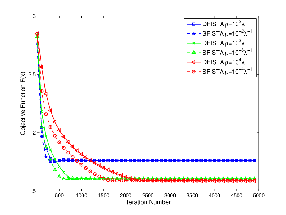
Fig. 3: The objective function for MRI reconstruction on Shepp Logan.
Refer to caption
Fig. 4: Reconstruction error for SFISTA and DFISTA with different parameters.

The next numerical experiment was performed on a noisy 256×256256\times 256 Shepp Logan phantom. The image scale was normalized to [0,1][0,1]. The additive noise followed a zero-mean Gaussian distribution with standard deviation σ=0.001\sigma=0.001. Due to the high cost of sampling in MRI, we only observed a limited number of radial lines of the phantom’s 2D discrete Fourier transform. The matrix 𝑫∗\bm{D}^{*} consists of all vertical and horizontal gradients, which leads to a sparse 𝑫∗​𝒙\bm{D}^{*}\bm{x}. We let λ=0.001\lambda=0.001 in the optimization. We tested this MRI scenario with μ\mu values of 10−2​λ−1,10−3​λ−1,10−4​λ−110^{-2}\lambda^{-1},10^{-3}\lambda^{-1},10^{-4}\lambda^{-1} for SFISTA and ρ=102λ,ρ=103λ,104λ\rho=10^{2}\lambda,\rho=10^{3}\lambda,10^{4}\lambda for DFISTA. We took the samples along 15 radial lines to test these two methods.

In Fig. 3 we plot the objective 12​‖𝑨​𝒙−𝒃‖22+λ​‖𝑫∗​𝒙‖1\frac{1}{2}\bm{\|}\bm{A}\bm{x}-\bm{b}\|_{2}^{2}+\lambda\|\bm{D}^{*}\bm{x}\|_{1} as a function of the iteration number. It can be seen that the objective function of SFISTA decreases more rapidly than DFISTA. Furthermore, with smaller ρ\rho and larger μ\mu, DFISTA and SFISTA converge faster. Then we computed the reconstruction error. Here we see that smaller μ\mu and larger ρ\rho lead to a more accurate reconstruction. We can see that SFISTA converges faster than DFISTA, which follows the convergence results in Section III.

Next, we compared SFISTA with the nonlinear conjugate gradient descend (CGD) algorithm proposed in [23]. The CGD also needs to introduce a smoothing transformation to approximate the term ‖𝑫∗​𝒙‖1\|\bm{D}^{*}\bm{x}\|_{1}, and in this simulation the Moreau envelop with μ=10−4​λ−1\mu=10^{-4}\lambda^{-1} was used to smooth this term. We can see from Fig. 5 that SFISTA converges faster than the CGD in terms of CPU time. CGD is slower because in each iteration, backtracking line-search is required, which reduces the algorithm efficiency.

Refer to caption
Fig. 5: Reconstruction error for SFISTA and CGD with respect to CPU time.

V-C Acceleration by Continuation

Algorithm 3: Continuation with SFISTA
Input: 𝒙\bm{x}, the starting parameter μ=μ0\mu=\mu_{0},
     the ending parameter μf\mu_{f} and γ>1\gamma>1.
Step 1. run SFISTA with μ\mu and initial point 𝒙\bm{x}.
Step 2. Get the solution 𝒙∗\bm{x}^{*} and let 𝒙=𝒙∗,μ=μ/γ\bm{x}=\bm{x}^{*},\mu=\mu/\gamma.
Until.  μ≤μf.\mu\leq\mu_{f}.

To accelerate convergence and increase the accuracy of reconstruction, we consider continuation on the parameter μ\mu for SFISTA, or on ρ\rho for DFISTA. From Theorem IV.1, we see that smaller μ\mu results in a smaller reconstruction error. At the same time, smaller μ\mu leads to a larger Lipschitz constant L∇FL_{\nabla F} in Theorem II.1, and thus results in slower convergence. The idea of continuation is to solve a sequence of similar problems while using the previous solution as a warm start. Taking the smoothing-based method as an example, we can run SFISTA with μ1≥μ2≥μ3,⋯≥μf\mu_{1}\geq\mu_{2}\geq\mu_{3},\dots\geq\mu_{f}. The continuation method is given in Algorithm 3. The algorithm for applying continuation on DFISTA is the same.

Refer to caption
Fig. 6: Convergence comparison among SFISTA with and without continuation, GIST and SALSA.
Refer to caption
Fig. 7: Reconstructed Shepp Logan with SFISTA using continuation.

We tested the algorithm on the Shepp Logan image from the previous subsection with the same setting, using SFISTA with μf=10−4​λ−1\mu_{f}=10^{-4}\lambda^{-1} and standard SFISTA with μ=10−4​λ−1\mu=10^{-4}\lambda^{-1}. We implemented the generalized iterative soft-thresholding algorithm (GIST) from [20]. We also included an ADMM-based method, i.e. the split augmented Lagrangian shrinkage algorithm (SALSA) [18]. SALSA requires solving the proximal operator of ‖𝑫∗​𝒙‖1\|\bm{D}^{*}\bm{x}\|_{1}, which is nontrivial. In this simulation, we implemented 4040 iterations of the Fast GP algorithm [25] to approximate this proximal operator. Without solving the proximal operator exactly, the ADMM-based method can converge very fast while the accuracy of reconstruction is compromised as we show in Figure 6. In this figure we plot the reconstruction error for these four algorithms. It also shows that continuation helps speed up the convergence and exhibits better performance then GIST. The reconstructed Shepp Logan phantom using continuation is presented in Fig. 7, with reconstruction error 3.17%3.17\%.

VI conclusion

In this paper, we proposed methods based on MFISTA to solve the analysis LASSO optimization problem. Since the proximal operator in MFISTA for ‖𝑫∗​𝒙‖1\|\bm{D}^{*}\bm{x}\|_{1} does not have a closed-form solution, we presented two methods, SFISTA and DFISTA, using smoothing and decomposition respectively, to transform the original sparse recovery problem into a smooth counterpart. We analyzed the convergence of SFISTA and DFISTA and showed that SFISTA converges faster in general nonsmooth optimization problems. We also derived a bound on the performance for both approaches assuming a tight frame and D-RIP. Our methods were demonstrated via several simulations. With the application of parameter continuation, these two algorithms are suitable to solve large scale problems.

Proof of Lemma IV.1: Without loss of generality we assume that ‖𝒖‖2=1\|\bm{u}\|_{2}=1 and ‖𝒗‖2=1\|\bm{v}\|_{2}=1. By the definition of D-RIP, we have

Re​⟨𝑨​𝒖,𝑨​𝒗⟩=\displaystyle\mathrm{Re}\langle\bm{A}\bm{u},\bm{A}\bm{v}\rangle= 14​{‖𝑨​𝒖+𝑨​𝒗‖22−‖𝑨​𝒖−𝑨​𝒗‖22}\displaystyle\frac{1}{4}\{\|\bm{A}\bm{u}+\bm{A}\bm{v}\|^{2}_{2}-\|\bm{A}\bm{u}-\bm{A}\bm{v}\|^{2}_{2}\}
≥\displaystyle\geq 14​{(1−σ2​s)​‖𝒖+𝒗‖22−(1+σ2​s)​‖𝒖−𝒗‖22}\displaystyle\frac{1}{4}\{(1-\sigma_{2s})\|\bm{u}+\bm{v}\|^{2}_{2}-(1+\sigma_{2s})\|\bm{u}-\bm{v}\|^{2}_{2}\}
=\displaystyle= −σ2​s+Re⁡⟨𝒖,𝒗⟩.\displaystyle-\sigma_{2s}+\mathrm{Re}\langle\bm{u},\bm{v}\rangle.

Now it is easy to extend this equation to get the desired result.

Proof of Lemma IV.2: From the definition of 𝒯j\mathcal{T}_{j} we have

‖𝑫𝒯j∗​𝒉‖2≤s−12​‖𝑫𝒯j−1∗​𝒉‖1\|\bm{D}^{*}_{\mathcal{T}_{j}}\bm{h}\|_{2}\leq s^{-\frac{1}{2}}\|\bm{D}^{*}_{\mathcal{T}_{j-1}}\bm{h}\|_{1}

for all j≥2j\geq 2. Summing j=2,3,…j=2,3,\ldots leads to

∑j≥2‖𝑫𝒯j∗​𝒉‖2≤s−12​∑j≥1‖𝑫𝒯j∗​𝒉‖1=s−12​‖𝑫𝒯c∗​𝒉‖1.\sum_{j\geq 2}\|\bm{D}^{*}_{\mathcal{T}_{j}}\bm{h}\|_{2}\leq s^{-\frac{1}{2}}\sum_{j\geq 1}\|\bm{D}^{*}_{\mathcal{T}_{j}}\bm{h}\|_{1}=s^{-\frac{1}{2}}\|\bm{D}^{*}_{\mathcal{T}^{c}}\bm{h}\|_{1}. (58)

Now, considering the fact that 𝑫\bm{D} is a tight frame, i.e., 𝑫​𝑫∗=𝑰\bm{D}\bm{D}^{*}=\bm{I}, and that the D-RIP holds,

R\displaystyle\mathrm{R} e⁡⟨𝑨​𝒉,𝑨​𝑫​𝑫𝒯01∗​𝒉⟩\displaystyle\mathrm{e}\langle\bm{A}\bm{h},\bm{A}\bm{D}\bm{D}^{*}_{\mathcal{T}_{01}}\bm{h}\rangle
=\displaystyle= Re⁡⟨𝑨​𝑫​𝑫𝒯01∗​𝒉,𝑨​𝑫​𝑫𝒯01∗​𝒉⟩+∑j≥2Re⁡⟨𝑨​𝑫​𝑫𝒯j∗​𝒉,𝑨​𝑫​𝑫𝒯01∗​𝒉⟩\displaystyle\mathrm{Re}\langle\bm{A}\bm{D}\bm{D}^{*}_{\mathcal{T}_{01}}\bm{h},\bm{A}\bm{D}\bm{D}^{*}_{\mathcal{T}_{01}}\bm{h}\rangle+\sum_{j\geq 2}\mathrm{Re}\langle\bm{A}\bm{D}\bm{D}^{*}_{\mathcal{T}_{j}}\bm{h},\bm{A}\bm{D}\bm{D}^{*}_{\mathcal{T}_{01}}\bm{h}\rangle
≥\displaystyle\geq (1−σ2​s)​‖𝑫​𝑫𝒯01∗​𝒉‖22+∑j≥2Re⁡⟨𝑨​𝑫​𝑫𝒯j∗​𝒉,𝑨​𝑫​𝑫𝒯0∗​𝒉⟩\displaystyle(1-\sigma_{2s})\|\bm{D}\bm{D}^{*}_{\mathcal{T}_{01}}\bm{h}\|^{2}_{2}+\sum_{j\geq 2}\mathrm{Re}\langle\bm{A}\bm{D}\bm{D}^{*}_{\mathcal{T}_{j}}\bm{h},\bm{A}\bm{D}\bm{D}^{*}_{\mathcal{T}_{0}}\bm{h}\rangle
+∑j≥2Re⟨𝑨𝑫𝑫𝒯j∗𝒉,𝑨𝑫𝑫𝒯1∗𝒉⟩\displaystyle+\sum_{j\geq 2}\mathrm{Re}\langle\bm{A}\bm{D}\bm{D}^{*}_{\mathcal{T}_{j}}\bm{h},\bm{A}\bm{D}\bm{D}^{*}_{\mathcal{T}_{1}}\bm{h}\rangle

Using the result from Lemma IV.1, we can bound the last two terms in the above inequality; hence, we derive

R\displaystyle\mathrm{R} e⁡⟨𝑨​𝒉,𝑨​𝑫​𝑫𝒯01∗​𝒉⟩\displaystyle\mathrm{e}\langle\bm{A}\bm{h},\bm{A}\bm{D}\bm{D}^{*}_{\mathcal{T}_{01}}\bm{h}\rangle
≥\displaystyle\geq (1−σ2​s)​‖𝑫​𝑫𝒯01∗​𝒉‖22+∑j≥2Re⁡⟨𝑫​𝑫𝒯j∗​𝒉,𝑫​𝑫𝒯0∗​𝒉⟩\displaystyle(1-\sigma_{2s})\|\bm{D}\bm{D}^{*}_{\mathcal{T}_{01}}\bm{h}\|^{2}_{2}+\sum_{j\geq 2}\mathrm{Re}\langle\bm{D}\bm{D}^{*}_{\mathcal{T}_{j}}\bm{h},\bm{D}\bm{D}^{*}_{\mathcal{T}_{0}}\bm{h}\rangle
+∑j≥2Re⟨𝑫𝑫𝒯j∗𝒉,𝑫𝑫𝒯1∗𝒉⟩\displaystyle+\sum_{j\geq 2}\mathrm{Re}\langle\bm{D}\bm{D}^{*}_{\mathcal{T}_{j}}\bm{h},\bm{D}\bm{D}^{*}_{\mathcal{T}_{1}}\bm{h}\rangle
−σ2​s|𝑫​𝑫𝒯0∗​𝒉|∑j≥22⁡‖𝑫​𝑫𝒯j∗​𝒉‖2\displaystyle-\sigma_{2s}\|\bm{D}\bm{D}^{*}_{\mathcal{T}_{0}}\bm{h}\|_{2}\sum_{j\geq 2}\|\bm{D}\bm{D}^{*}_{\mathcal{T}_{j}}\bm{h}\|_{2}
−σ2​s|𝑫​𝑫𝒯1∗​𝒉|∑j≥22⁡‖𝑫​𝑫𝒯j∗​𝒉‖2\displaystyle-\sigma_{2s}\|\bm{D}\bm{D}^{*}_{\mathcal{T}_{1}}\bm{h}\|_{2}\sum_{j\geq 2}\|\bm{D}\bm{D}^{*}_{\mathcal{T}_{j}}\bm{h}\|_{2}
=\displaystyle= (1−σ2​s)​‖𝑫​𝑫𝒯01∗​𝒉‖22+Re⁡⟨∑j≥2𝑫​𝑫𝒯j∗​𝒉,𝑫​𝑫𝒯01∗​𝒉⟩\displaystyle(1-\sigma_{2s})\|\bm{D}\bm{D}^{*}_{\mathcal{T}_{01}}\bm{h}\|^{2}_{2}+\mathrm{Re}\left\langle\sum_{j\geq 2}\bm{D}\bm{D}^{*}_{\mathcal{T}_{j}}\bm{h},\bm{D}\bm{D}^{*}_{\mathcal{T}_{01}}\bm{h}\right\rangle
−σ2​s(∥𝑫𝑫𝒯0∗𝒉∥2+∥𝑫𝑫𝒯1∗𝒉∥2)∑j≥2∥𝑫𝑫𝒯j∗𝒉∥2\displaystyle-\sigma_{2s}(\|\bm{D}\bm{D}^{*}_{\mathcal{T}_{0}}\bm{h}\|_{2}+\|\bm{D}\bm{D}^{*}_{\mathcal{T}_{1}}\bm{h}\|_{2})\sum_{j\geq 2}\|\bm{D}\bm{D}^{*}_{\mathcal{T}_{j}}\bm{h}\|_{2} (59)

By definition of 𝒯j\mathcal{T}_{j}, we have

Re⁡⟨∑j≥2𝑫​𝑫𝒯j∗​𝒉,𝑫​𝑫𝒯01∗​𝒉⟩\displaystyle\mathrm{Re}\left\langle\sum_{j\geq 2}\bm{D}\bm{D}^{*}_{\mathcal{T}_{j}}\bm{h},\bm{D}\bm{D}^{*}_{\mathcal{T}_{01}}\bm{h}\right\rangle =Re⁡⟨𝒉−𝑫​𝑫𝒯01∗​𝒉,𝑫​𝑫𝒯01∗​𝒉⟩\displaystyle=\mathrm{Re}\langle\bm{h}-\bm{D}\bm{D}^{*}_{\mathcal{T}_{01}}\bm{h},\bm{D}\bm{D}^{*}_{\mathcal{T}_{01}}\bm{h}\rangle
=‖𝑫𝒯01∗​𝒉‖22−‖𝑫​𝑫𝒯01∗​𝒉‖22.\displaystyle=\|\bm{D}^{*}_{\mathcal{T}_{01}}\bm{h}\|^{2}_{2}-\|\bm{D}\bm{D}^{*}_{\mathcal{T}_{01}}\bm{h}\|^{2}_{2}.

Combining this equation with (59) results in

R\displaystyle\mathrm{R} e⁡⟨𝑨​𝒉,𝑨​𝑫​𝑫𝒯01∗​𝒉⟩\displaystyle\mathrm{e}\langle\bm{A}\bm{h},\bm{A}\bm{D}\bm{D}^{*}_{\mathcal{T}_{01}}\bm{h}\rangle
≥\displaystyle\geq ‖𝑫​𝑫𝒯01∗​𝒉‖22−σ2​s​‖𝑫​𝑫𝒯01∗​𝒉‖22+‖𝑫𝒯01∗​𝒉‖22−‖𝑫​𝑫𝒯01∗​𝒉‖22\displaystyle\|\bm{D}\bm{D}^{*}_{\mathcal{T}_{01}}\bm{h}\|^{2}_{2}-\sigma_{2s}\|\bm{D}\bm{D}^{*}_{\mathcal{T}_{01}}\bm{h}\|^{2}_{2}+\|\bm{D}^{*}_{\mathcal{T}_{01}}\bm{h}\|^{2}_{2}-\|\bm{D}\bm{D}^{*}_{\mathcal{T}_{01}}\bm{h}\|^{2}_{2}
−σ2​s(∥𝑫𝑫𝒯0∗𝒉∥2+∥𝑫𝑫𝒯1∗𝒉∥2)∑j≥2∥𝑫𝑫𝒯j∗𝒉∥2.\displaystyle-\sigma_{2s}(\|\bm{D}\bm{D}^{*}_{\mathcal{T}_{0}}\bm{h}\|_{2}+\|\bm{D}\bm{D}^{*}_{\mathcal{T}_{1}}\bm{h}\|_{2})\sum_{j\geq 2}\|\bm{D}\bm{D}^{*}_{\mathcal{T}_{j}}\bm{h}\|_{2}.

Using the fact that when 𝑫\bm{D} is a tight frame, ‖𝑫​𝑫𝒯01∗​𝒉‖2≤‖𝑫𝒯01∗​𝒉‖2\|\bm{D}\bm{D}^{*}_{\mathcal{T}_{01}}\bm{h}\|_{2}\leq\|\bm{D}^{*}_{\mathcal{T}_{01}}\bm{h}\|_{2}, we have

R\displaystyle\mathrm{R} e⁡⟨𝑨​𝒉,𝑨​𝑫​𝑫𝒯01∗​𝒉⟩\displaystyle\mathrm{e}\langle\bm{A}\bm{h},\bm{A}\bm{D}\bm{D}^{*}_{\mathcal{T}_{01}}\bm{h}\rangle
≥\displaystyle\geq (1−σ2​s)​‖𝑫𝒯01∗​𝒉‖22−σ2​s​(‖𝑫𝒯0∗​𝒉‖2+‖𝑫𝒯1∗​𝒉‖2)​∑j≥2‖𝑫𝒯j∗​𝒉‖2.\displaystyle(1-\sigma_{2s})\|\bm{D}^{*}_{\mathcal{T}_{01}}\bm{h}\|^{2}_{2}-\sigma_{2s}(\|\bm{D}^{*}_{\mathcal{T}_{0}}\bm{h}\|_{2}+\|\bm{D}^{*}_{\mathcal{T}_{1}}\bm{h}\|_{2})\sum_{j\geq 2}\|\bm{D}^{*}_{\mathcal{T}_{j}}\bm{h}\|_{2}.

Since ‖𝑫𝒯0∗​𝒉‖2+‖𝑫𝒯1∗​𝒉‖2≤2​‖𝑫𝒯01∗​𝒉‖2\|\bm{D}^{*}_{\mathcal{T}_{0}}\bm{h}\|_{2}+\|\bm{D}^{*}_{\mathcal{T}_{1}}\bm{h}\|_{2}\leq\sqrt{2}\|\bm{D}^{*}_{\mathcal{T}_{01}}\bm{h}\|_{2} (becuase 𝒯0\mathcal{T}_{0} and 𝒯1\mathcal{T}_{1} are disjoint), we conclude that

R\displaystyle\mathrm{R} e⁡⟨𝑨​𝒉,𝑨​𝑫​𝑫𝒯01∗​𝒉⟩\displaystyle\mathrm{e}\langle\bm{A}\bm{h},\bm{A}\bm{D}\bm{D}^{*}_{\mathcal{T}_{01}}\bm{h}\rangle
≥\displaystyle\geq (1−σ2​s)​‖𝑫𝒯01∗​𝒉‖22−2​σ2​s​‖𝑫𝒯01∗​𝒉‖2​∑j≥2‖𝑫𝒯j∗​𝒉‖2,\displaystyle(1-\sigma_{2s})\|\bm{D}^{*}_{\mathcal{T}_{01}}\bm{h}\|^{2}_{2}-\sqrt{2}\sigma_{2s}\|\bm{D}^{*}_{\mathcal{T}_{01}}\bm{h}\|_{2}\sum_{j\geq 2}\|\bm{D}^{*}_{\mathcal{T}_{j}}\bm{h}\|_{2},

which along with inequality (58) yields the desired result given by

R\displaystyle\mathrm{R} e⁡⟨𝑨​𝒉,𝑨​𝑫​𝑫𝒯01∗​𝒉⟩\displaystyle\mathrm{e}\langle\bm{A}\bm{h},\bm{A}\bm{D}\bm{D}^{*}_{\mathcal{T}_{01}}\bm{h}\rangle
≥\displaystyle\geq (1−σ2​s)​‖𝑫𝒯01∗​𝒉‖22−2​s−12​σ2​s​‖𝑫𝒯01∗​𝒉‖2​‖𝑫𝒯c∗​𝒉‖1.\displaystyle(1-\sigma_{2s})\|\bm{D}^{*}_{\mathcal{T}_{01}}\bm{h}\|^{2}_{2}-\sqrt{2}s^{-\frac{1}{2}}\sigma_{2s}\|\bm{D}^{*}_{\mathcal{T}_{01}}\bm{h}\|_{2}\|\bm{D}^{*}_{\mathcal{T}^{c}}\bm{h}\|_{1}.

Proof of Lemma IV.3: The subgradient optimality condition for RALASSO (5) can be stated as

𝑨∗​(𝑨​𝒙^ρ−𝒃)+ρ​𝑫​(𝑫∗​𝒙^ρ−𝒛^ρ)=0,\bm{A}^{*}(\bm{A}\hat{\bm{x}}_{\rho}-\bm{b})+\rho\bm{D}(\bm{D}^{*}\hat{\bm{x}}_{\rho}-\hat{\bm{z}}_{\rho})=0, (60)
λ​𝒗+ρ⁡(𝒛^ρ−𝑫∗​𝒙^ρ)=0,\lambda\bm{v}+\rho(\hat{\bm{z}}_{\rho}-\bm{D}^{*}\hat{\bm{x}}_{\rho})=0, (61)

where 𝒗\bm{v} is a subgradient of the function ‖𝒛‖1\|\bm{z}\|_{1} and consequently ‖𝒗‖∞≤1\|\bm{v}\|_{\infty}\leq 1. Combining (60) and (61), we have

𝑨∗​(𝑨​𝒙^ρ−𝒃)=λ​𝑫​𝒗.\bm{A}^{*}(\bm{A}\hat{\bm{x}}_{\rho}-\bm{b})=\lambda\bm{D}\bm{v}.

Multiplying both sides by 𝑫∗\bm{D}^{*}, we get

‖𝑫∗​𝑨∗​(𝑨​𝒙^ρ−𝒃)‖∞\displaystyle\|\bm{D}^{*}\bm{A}^{*}(\bm{A}\hat{\bm{x}}_{\rho}-\bm{b})\|_{\infty}
=λ​‖𝑫∗​𝑫​𝒗‖∞≤λ​‖𝑫∗​𝑫‖∞,∞=λ​‖𝑫∗​𝑫‖1,1.\displaystyle=\lambda\|\bm{D}^{*}\bm{D}\bm{v}\|_{\infty}\leq\lambda\|\bm{D}^{*}\bm{D}\|_{\infty,\infty}=\lambda\|\bm{D}^{*}\bm{D}\|_{1,1}. (62)

The first inequality follows from the fact that ‖𝒗‖∞≤1\|\bm{v}\|_{\infty}\leq 1. With the assumption that ‖𝑫∗​𝑨∗​𝒘‖∞≤λ2\|\bm{D}^{*}\bm{A}^{*}\bm{w}\|_{\infty}\leq\frac{\lambda}{2}, and the triangle inequality, we have

‖𝑫∗​𝑨∗​𝑨​𝒉‖∞\displaystyle\|\bm{D}^{*}\bm{A}^{*}\bm{A}\bm{h}\|_{\infty}
≤‖𝑫∗​𝑨∗​(𝑨​𝒙−𝒃)‖∞+‖𝑫∗​𝑨∗​(𝑨​𝒙^ρ−𝒃)‖∞\displaystyle\leq\|\bm{D}^{*}\bm{A}^{*}(\bm{A}\bm{x}-\bm{b})\|_{\infty}+\|\bm{D}^{*}\bm{A}^{*}(\bm{A}\hat{\bm{x}}_{\rho}-\bm{b})\|_{\infty}
≤(12+‖𝑫∗​𝑫‖1,1)​λ.\displaystyle\leq\left(\frac{1}{2}+\|\bm{D}^{*}\bm{D}\|_{1,1}\right)\lambda. (63)

Proof of Lemma IV.4: Since 𝒙^ρ\hat{\bm{x}}_{\rho} and 𝒛^ρ\hat{\bm{z}}_{\rho} solve the optimization problem RALASSO (5), we have,

12​‖𝑨​𝒙^ρ−𝒃‖22+λ​‖𝒛^ρ‖1+12​ρ​‖𝑫∗​𝒙^ρ−𝒛^ρ‖22\displaystyle\frac{1}{2}\|\bm{A}\hat{\bm{x}}_{\rho}-\bm{b}\|^{2}_{2}+\lambda\|\hat{\bm{z}}_{\rho}\|_{1}+\frac{1}{2}\rho\|\bm{D}^{*}\hat{\bm{x}}_{\rho}-\hat{\bm{z}}_{\rho}\|^{2}_{2}
≤12​‖𝑨​𝒙−𝒃‖22+λ​‖𝑫∗​𝒙‖1.\displaystyle\leq\frac{1}{2}\|\bm{A}\bm{x}-\bm{b}\|_{2}^{2}+\lambda\|\bm{D}^{*}\bm{x}\|_{1}.

Since 𝒃=𝑨​𝒙+𝒘\bm{b}=\bm{A}\bm{x}+\bm{w} and 𝒉=𝒙^ρ−𝒙\bm{h}=\hat{\bm{x}}_{\rho}-\bm{x}, it follows that

12​‖𝑨​𝒉−𝒘‖22+λ​‖𝒛^ρ‖1+12​ρ​‖𝑫∗​𝒙^ρ−𝒛^ρ‖22\displaystyle\frac{1}{2}\|\bm{A}\bm{h}-\bm{w}\|_{2}^{2}+\lambda\|\hat{\bm{z}}_{\rho}\|_{1}+\frac{1}{2}\rho\|\bm{D}^{*}\hat{\bm{x}}_{\rho}-\hat{\bm{z}}_{\rho}\|^{2}_{2}
≤12​‖𝒘‖22+λ​‖𝑫∗​𝒙‖1.\displaystyle\leq\frac{1}{2}\|\bm{w}\|_{2}^{2}+\lambda\|\bm{D}^{*}\bm{x}\|_{1}.

Expanding and rearranging the terms in the above equation, we get

12​‖𝑨​𝒉‖22+λ​‖𝒛^ρ‖1+12​ρ​‖𝑫∗​𝒙^ρ−𝒛^ρ‖22\displaystyle\frac{1}{2}\|\bm{A}\bm{h}\|_{2}^{2}+\lambda\|\hat{\bm{z}}_{\rho}\|_{1}+\frac{1}{2}\rho\|\bm{D}^{*}\hat{\bm{x}}_{\rho}-\hat{\bm{z}}_{\rho}\|_{2}^{2}
≤Re⁡⟨𝑨​𝒉,𝒘⟩+λ​‖𝑫∗​𝒙‖1,\displaystyle\leq\mathrm{Re}\langle\bm{A}\bm{h},\bm{w}\rangle+\lambda\|\bm{D}^{*}\bm{x}\|_{1},

Using (61) to replace the terms with 𝒛^ρ\hat{\bm{z}}_{\rho}, we have

12​‖𝑨​𝒉‖22+λ​‖𝑫∗​𝒙^ρ−λρ​𝒗‖1+12​ρ​‖λρ​𝒗‖22\displaystyle\frac{1}{2}\|\bm{A}\bm{h}\|_{2}^{2}+\lambda\left\|\bm{D}^{*}\hat{\bm{x}}_{\rho}-\frac{\lambda}{\rho}\bm{v}\right\|_{1}+\frac{1}{2}\rho\left\|\frac{\lambda}{\rho}\bm{v}\right\|_{2}^{2}
≤Re⁡⟨𝑨​𝒉,𝒘⟩+λ​‖𝑫∗​𝒙‖1.\displaystyle\leq\mathrm{Re}\langle\bm{A}\bm{h},\bm{w}\rangle+\lambda\|\bm{D}^{*}\bm{x}\|_{1}.

Since ‖𝑫∗​𝒙^ρ−λρ​𝒗‖1≥‖𝑫∗​𝒙^ρ‖1−λρ​‖𝒗‖1\|\bm{D}^{*}\hat{\bm{x}}_{\rho}-\frac{\lambda}{\rho}\bm{v}\|_{1}\geq\|\bm{D}^{*}\hat{\bm{x}}_{\rho}\|_{1}-\frac{\lambda}{\rho}\|\bm{v}\|_{1}, we have

12​‖𝑨​𝒉‖22+λ​‖𝑫∗​𝒙^ρ‖1\displaystyle\frac{1}{2}\|\bm{A}\bm{h}\|_{2}^{2}+\lambda\|\bm{D}^{*}\hat{\bm{x}}_{\rho}\|_{1}
≤λ2ρ​‖𝒗‖1−λ22​ρ​‖𝒗‖22+Re⁡⟨𝑨​𝒉,𝒘⟩+λ​‖𝑫∗​𝒙‖1\displaystyle\leq\frac{\lambda^{2}}{\rho}\|\bm{v}\|_{1}-\frac{\lambda^{2}}{2\rho}\|\bm{v}\|_{2}^{2}+\mathrm{Re}\langle\bm{A}\bm{h},\bm{w}\rangle+\lambda\|\bm{D}^{*}\bm{x}\|_{1}
≤λ2​p2​ρ+Re⁡⟨𝑨​𝒉,𝒘⟩+λ​‖𝑫∗​𝒙‖1.\displaystyle\leq\frac{\lambda^{2}p}{2\rho}+\mathrm{Re}\langle\bm{A}\bm{h},\bm{w}\rangle+\lambda\|\bm{D}^{*}\bm{x}\|_{1}. (64)

The second inequality follows from the fact that λ2ρ​‖𝒗‖1−λ22​ρ​‖𝒗‖22\frac{\lambda^{2}}{\rho}\|\bm{v}\|_{1}-\frac{\lambda^{2}}{2\rho}\|\bm{v}\|_{2}^{2} is maximized when every element of 𝒗∈ℝp\bm{v}\in\mathbb{R}^{p} is 11. Now, with the assumption that 𝑫\bm{D} is a tight frame, we have the following relation:

Re⁡⟨𝑨​𝒉,𝒘⟩+λ​‖𝑫∗​𝒙‖1=\displaystyle\mathrm{Re}\langle\bm{A}\bm{h},\bm{w}\rangle+\lambda\|\bm{D}^{*}\bm{x}\|_{1}= Re⁡⟨𝑫∗​𝒉,𝑫∗​𝑨∗​𝒘⟩+λ​‖𝑫∗​𝒙‖1\displaystyle\mathrm{Re}\langle\bm{D}^{*}\bm{h},\bm{D}^{*}\bm{A}^{*}\bm{w}\rangle+\lambda\|\bm{D}^{*}\bm{x}\|_{1}
≤\displaystyle\leq ‖𝑫∗​𝒉‖1​‖𝑫∗​𝑨∗​𝒘‖∞+λ​‖𝑫∗​𝒙‖1.\displaystyle\|\bm{D}^{*}\bm{h}\|_{1}\|\bm{D}^{*}\bm{A}^{*}\bm{w}\|_{\infty}+\lambda\|\bm{D}^{*}\bm{x}\|_{1}.

This inequality follows from the fact that Re⁡⟨𝒙,𝒚⟩≤‖⟨𝒙,𝒚⟩‖≤‖𝒙‖1​‖𝒚‖∞\mathrm{Re}\langle\bm{x},\bm{y}\rangle\leq\|\langle\bm{x},\bm{y}\rangle\|\leq\|\bm{x}\|_{1}\|\bm{y}\|_{\infty}. Using the assumption that ‖𝑫∗​𝑨∗​𝒘‖∞≤λ2\|\bm{D}^{*}\bm{A}^{*}\bm{w}\|_{\infty}\leq\frac{\lambda}{2}, we get

Re⁡⟨𝑨​𝒉,𝒘⟩+λ​‖𝑫∗​𝒙‖1≤λ2​‖𝑫∗​𝒉‖1+λ​‖𝑫∗​𝒙‖1.\mathrm{Re}\langle\bm{A}\bm{h},\bm{w}\rangle+\lambda\|\bm{D}^{*}\bm{x}\|_{1}\leq\frac{\lambda}{2}\|\bm{D}^{*}\bm{h}\|_{1}+\lambda\|\bm{D}^{*}\bm{x}\|_{1}. (65)

Applying inequalities (64) and (65), we have

λ​‖𝑫∗​𝒙^ρ‖1≤\displaystyle\lambda\|\bm{D}^{*}\hat{\bm{x}}_{\rho}\|_{1}\leq 12​‖𝑨​𝒉‖22+λ​‖𝑫∗​𝒙^ρ‖1\displaystyle\frac{1}{2}\|\bm{A}\bm{h}\|_{2}^{2}+\lambda\|\bm{D}^{*}\hat{\bm{x}}_{\rho}\|_{1}
≤\displaystyle\leq λ22​ρ​p+Re⁡⟨𝑨​𝒉,𝒘⟩+λ​‖𝑫∗​𝒙‖1\displaystyle\frac{\lambda^{2}}{2\rho}p+\mathrm{Re}\langle\bm{A}\bm{h},\bm{w}\rangle+\lambda\|\bm{D}^{*}\bm{x}\|_{1}
≤\displaystyle\leq λ22​ρ​p+λ2​‖𝑫∗​𝒉‖1+λ​‖𝑫∗​𝒙‖1,\displaystyle\frac{\lambda^{2}}{2\rho}p+\frac{\lambda}{2}\|\bm{D}^{*}\bm{h}\|_{1}+\lambda\|\bm{D}^{*}\bm{x}\|_{1},

which is the same as,

‖𝑫∗​𝒙^ρ‖1≤λ2​ρ​p+12​‖𝑫∗​𝒉‖1+‖𝑫∗​𝒙‖1.\|\bm{D}^{*}\hat{\bm{x}}_{\rho}\|_{1}\leq\frac{\lambda}{2\rho}p+\frac{1}{2}\|\bm{D}^{*}\bm{h}\|_{1}+\|\bm{D}^{*}\bm{x}\|_{1}.

Since we have 𝒉=𝒙^ρ−𝒙\bm{h}=\hat{\bm{x}}_{\rho}-\bm{x}, it follows that

‖𝑫∗​𝒉+𝑫∗​𝒙‖1≤λ2​ρ​p+12​‖𝑫∗​𝒉‖1+‖𝑫∗​𝒙‖1,\|\bm{D}^{*}\bm{h}+\bm{D}^{*}\bm{x}\|_{1}\leq\frac{\lambda}{2\rho}p+\frac{1}{2}\|\bm{D}^{*}\bm{h}\|_{1}+\|\bm{D}^{*}\bm{x}\|_{1},

and hence

‖𝑫𝒯∗​𝒉+𝑫𝒯∗​𝒙‖1+‖𝑫𝒯c∗​𝒉+𝑫𝒯c∗​𝒙‖1\displaystyle\|\bm{D}^{*}_{\mathcal{T}}\bm{h}+\bm{D}_{\mathcal{T}}^{*}\bm{x}\|_{1}+\|\bm{D}^{*}_{\mathcal{T}^{c}}\bm{h}+\bm{D}_{\mathcal{T}^{c}}^{*}\bm{x}\|_{1}
≤λ2​ρ​p+12​‖𝑫𝒯∗​𝒉‖1+12​‖𝑫𝒯c∗​𝒉‖1+‖𝑫𝒯∗​𝒙‖1+‖𝑫𝒯c∗​𝒙‖1.\displaystyle\leq\frac{\lambda}{2\rho}p+\frac{1}{2}\|\bm{D}_{\mathcal{T}}^{*}\bm{h}\|_{1}+\frac{1}{2}\|\bm{D}_{\mathcal{T}^{c}}^{*}\bm{h}\|_{1}+\|\bm{D}_{\mathcal{T}}^{*}\bm{x}\|_{1}+\|\bm{D}_{\mathcal{T}^{c}}^{*}\bm{x}\|_{1}.

Applying the triangle inequality to the left handside of above inequality, we results in

−‖𝑫𝒯∗​𝒉‖1+‖𝑫𝒯∗​𝒙‖1+‖𝑫𝒯c∗​𝒉‖1−‖𝑫𝒯c∗​𝒙‖1\displaystyle-\|\bm{D}^{*}_{\mathcal{T}}\bm{h}\|_{1}+\|\bm{D}_{\mathcal{T}}^{*}\bm{x}\|_{1}+\|\bm{D}^{*}_{\mathcal{T}^{c}}\bm{h}\|_{1}-\|\bm{D}_{\mathcal{T}^{c}}^{*}\bm{x}\|_{1}
≤λ2​ρ​p+12​‖𝑫𝒯∗​𝒉‖1+12​‖𝑫𝒯c∗​𝒉‖1+‖𝑫𝒯∗​𝒙‖1+‖𝑫𝒯c∗​𝒙‖1.\displaystyle\leq\frac{\lambda}{2\rho}p+\frac{1}{2}\|\bm{D}_{\mathcal{T}}^{*}\bm{h}\|_{1}+\frac{1}{2}\|\bm{D}_{\mathcal{T}^{c}}^{*}\bm{h}\|_{1}+\|\bm{D}_{\mathcal{T}}^{*}\bm{x}\|_{1}+\|\bm{D}_{\mathcal{T}^{c}}^{*}\bm{x}\|_{1}.

After rearranging the terms, we have the following cone constraint,

‖𝑫𝒯c∗​𝒉‖1≤λρ​p+3​‖𝑫𝒯∗​𝒉‖1+4​‖𝑫𝒯c∗​𝒙‖1.\|\bm{D}^{*}_{\mathcal{T}^{c}}\bm{h}\|_{1}\leq\frac{\lambda}{\rho}p+3\|\bm{D}^{*}_{\mathcal{T}}\bm{h}\|_{1}+4\|\bm{D}^{*}_{\mathcal{T}^{c}}\bm{x}\|_{1}. (66)

References

  • [1] E. J. Candès and M. B. Wakin, “An introduction to compressive sampling,” IEEE Signal Process. Mag., vol. 25, no. 2, pp. 21 –30, Mar. 2008.
  • [2] E. J. Candès, J. Romberg, and T. Tao, “Robust uncertainty principles: exact signal reconstruction from highly incomplete frequency information,” IEEE Trans. Inf. Theory, vol. 52, no. 2, pp. 489 – 509, Feb. 2006.
  • [3] E. J. Candès and T. Tao, “Near-optimal signal recovery from random projections: Universal encoding strategies?” IEEE Trans. Inf. Theory, vol. 52, no. 12, pp. 5406 –5425, Dec. 2006.
  • [4] Y. C. Eldar and G. Kutyniok, Compressed Sensing: Theory and Applications. Cambridge University Press, 2012.
  • [5] T. Blumensath and M. E. Davies, “Iterative hard thresholding for compressed sensing,” Applied and Computational Harmonic Analysis, vol. 27, no. 3, pp. 265 – 274, 2009. [Online]. Available: http://www.sciencedirect.com/science/article/pii/S1063520309000384
  • [6] J. A. Tropp and A. C. Gilbert, “Signal recovery from random measurements via orthogonal matching pursuit,” IEEE Trans. Inf. Theory, vol. 53, no. 12, pp. 4655 –4666, Dec. 2007.
  • [7] S. S. Chen, D. L. Donoho, and M. A. Saunders, “Atomic decomposition by basis pursuit,” SIAM Rev., vol. 43, no. 3, pp. 129 –159, Mar. 2001.
  • [8] T. Hastie, R. Tibshirani, and J. Friedman, The Elements of Statistical Learning: Data, Mining, Intereference, and Prediction, 2nd ed. New York: Springer, 2009.
  • [9] E. J. Candès, “The restricted isometry property and its implications for compressed sensing,” C. R. Acad. Sci. Paris, Ser. I, 2008.
  • [10] P. Bickel, Y. Ritov, and A. Tsybakov, “Simultaneous analysis of lasso and dantzig selector,” Ann. Statist., 2009.
  • [11] T. Blumensath and M. E. Davies, “Normalized iterative hard thresholding: Guaranteed stability and performance,” IEEE J. Sel. Topics Signal Process., vol. 4, no. 2, pp. 298–309, 2010.
  • [12] E. J. Candès, Y. C. Eldar, D. Needell, and P. Randall, “Compressed sensing with coherent and redundant dictionaries,” Appl. Comput. Harmon. Anal., 2011.
  • [13] S. Nam, M. E. Davies, M. Elad, and R. Gribonval, “The cosparse analysis model and algorithms,” Applied and Computational Harmonic Analysis, vol. 34, no. 1, pp. 30 – 56, 2013. [Online]. Available: http://www.sciencedirect.com/science/article/pii/S1063520312000450
  • [14] T. Peleg and M. Elad, “Performance guarantees of the thresholding algorithm for the cosparse analysis model,” IEEE Trans. Ind. Informat., vol. 59, no. 3, pp. 1832–1845, 2013.
  • [15] R. Giryes, S. Nam, M. Elad, R. Gribonval, and M. E. Davies, “Greedy-like algorithms for the cosparse analysis model,” Linear Algebra and its Applications, no. 0, pp. –, 2013. [Online]. Available: http://www.sciencedirect.com/science/article/pii/S0024379513001870
  • [16] S. Boyd and L. Vandenberghe, Convex Optimization. Cambridge University Press, 2004.
  • [17] S. Boyd, N. Parikh, E. Chu, B. Peleato, and J. Eckstein, “Distributed optimization and statistical learning via alternating direction method of multipliers,” in Found. Trends Mach Learning, vol. 3, 2010, pp. 1–122.
  • [18] M. V. Afonso, J. M. Bioucas-Dias, and M. A. T. Figueiredo, “Fast image recovery using variable splitting and constrained optimization,” IEEE Trans. Image Process., vol. 19, no. 9, pp. 2345–2356, 2010.
  • [19] A. Beck and M. Teboulle, “A fast iterative shrinkage-thresholding algorithm for linear inverse problems,” SIAM. on Imaging Sciences 2(1), 2009.
  • [20] I. Loris and C. Verhoeven, “On a generalization of the iterative soft-thresholding algorithm for the case of non-separable penalty,” Inverse Problems, vol. 27, no. 12, 2011.
  • [21] S. Becker, J. Bobin, and E. J. Candès, “Nesta: a fast and accurate first-order method for sparse recovery,” SIAM J. on Imaging Sciences 4(1), pp. 1–39.
  • [22] Y. E. Nesterov, “Smooth minimization of non-smooth functions,” Math. Program, vol. 103, no. 1, pp. 127–152, 2005.
  • [23] M. Lustig, D. Donoho, and J. M. Pauly, “Sparse MRI: The application of compressed sensing for rapid MR imaging,” Magnetic Resonance in Medicine, vol. 58, no. 6, pp. 1182–1195, 2007.
  • [24] A. Beck and M. Teboulle, “Smoothing and first order methods: a unified framework,” SIAM J. Optim, vol. 22, no. 2, pp. 557–580, 2012.
  • [25] ——, “Fast gradient-based algorithms for constrained total variation image denoising and deblurring problems,” IEEE Trans. Image Process., vol. 18, no. 11, pp. 2419–2434, Nov.
  • [26] R. Courant, “Variational methods for the solution of problems with equilibrium and vibration,” Bull. Amer. Math. Soc., vol. 49, pp. 1–23, 1943.
  • [27] Y. Wang, J. Yang, W. Yin, and Y. Zhang, “A new alternating minimization algorithm for total variation image reconstruction,” SIAM J. Imaging Sciences, vol. 1, no. 3, pp. 248–272, 2008.
  • [28] J. Lin and S. Li, “Sparse recovery with coherent tight frame via analysis dantzig selector and analysis lasso,” arXiv:1301.3248.
  • [29] J. J. Moreau, “Proximitéet dualité dans un espace hilbertien,” Bull. Soc. Math. France, vol. 93, pp. 273–299, 1965.
  • [30] ——, “Fonctions convexes duales et points proximaux dans un espace hilbertien.” Comptes Rendus de l’Académie des Sciences (Paris), Série A, vol. 255, pp. 2897–2899, 1962.
  • [31] H. H. Bauschke and P. L. Combettes, Convex Analysis and Monotone Operator Theory in Hilbert Space. Springer, 2011.
  • [32] A. Beck and M. Teboulle, “Gradient-based algorithms with applications to signal recovery problems,” in Convex Optimization in Signal Processing and Communications, D. Palomar and Y. Eldar, Eds. Cambridge University Press, 2009, pp. 139–162.
  • [33] Y. E. Nesterov, “A method for solving the convex programming problem with convergence rate O⁡(1/k2)O(1/k^{2}),” Dokl. Akad. Nauk SSSR, vol. 269, no. 3, pp. 543–547, 1983.
  • [34] P. J. Huber, “Robust estimation of a location parameter,” Ann. Math. Statist., vol. 35, pp. 73–101, 1964.
  • [35] D. Needell and J. A. Tropp, “Cosamp: Iterative signal recovery from noisy samples,” Appl. Comput. Harmon. Anal, vol. 26, no. 3, pp. 301–321, 2008.
  • [36] M. A. T. Figueiredo, R. D. Nowak, and S. J. Wright, “Gradient projection for sparse reconstruction: Application to compressed sensing and other inverse problems,” Selected Topics in Signal Processing, IEEE Journal of, vol. 1, no. 4, pp. 586–597, 2007.