ALBERT-LUDWIGS-UNIVERSITÄT, FREIBURG IM BREISGAU
FAKULTÄT FÜR PHYSIK
DIPLOMARBEIT / DIPLOMA THESIS
The calibration of the vector
polarimeter POLIS
CHRISTIAN BECK
![[Uncaptioned image]](1308.4954v1/polis_logo.png)
angefertigt am
Kiepenheuer-Institut für Sonnenphysik, Freiburg
April 2002
Abstract
In this diploma thesis, the calibration of the new vector polarimeter
POLIS will be described. The instrument is built by the
Kiepenheuer-Institut für Sonnenphysik (KIS, Freiburg, Germany) in
cooperation with the High Altitude Observatory (HAO, Boulder, USA). It
will be operated at the German Vacuum Tower Telescope (VTT) in Tenerife.
The instrument yields simultaneously the polarization state of light in
two spectral ranges at 396 nm and 630 nm. The
measurement is performed with a rotating retarder, which modulates the incident
polarization. The modulation is transformed into a varying intensity
through polarizing beamsplitters. The demodulation uses a weighted
integration scheme to obtain the full Stokes vector of the radiation.
To achieve a sufficient polarimetric accuracy of 0.1 of
the continuum intensity, it is necessary to calibrate the polarimeter and
remove the instrumental polarization due to the telescope.
The calibration of the polarimeter is performed through the evaluation of the calibration data set. This data is produced with a calibration unit consisting of a linear polarizer and a retarder. Both elements are placed in rotatable mounts and can be steered by remote control. The calibration unit will be placed inside the vacuum tank at the VTT Tenerife.
The polarimeter response function or X-matrix can be determined
from a comparison between created input and measured output. The
calibration data images have to be corrected for the detector properties
before, which can be achieved with additional flatfield and dark current
data. The application of the inverse matrix X-1 removes the
properties of the polarimeter from measured data.
The instrumental polarization of the telescope, which changes the Stokes
vector incident from the sun, will be removed through
the usage of a model of the polarimetric properties of the telescope. The
optical elements in the telescope are modelled by appropriate
Mueller matrices with free parameters. To calculate the total optical
train, it is necessary to consider the specific geometry of the light
path at each moment of time. For this purpose a numerical approach was
developed that can be applied to other optical setups as well, if the
beam path is known. The free parameters in the telescope model will be
derived from a least-square-fit to telescope calibration
data. Similar to the polarimeter calibration, known input states can be
created with an array of polarizing sheets, which can be placed either
on top of the first mirror or on top of the entrance window of the
vacuum tank. The corresponding measurements should allow to obtain
the required parameter values, after the polarimeter properties have been
removed by the application of X-1.
Due to the delayed setup of POLIS, data from the Advanced Stokes Polarimeter (ASP) is used to display the calibration steps and probable results. The last chapter presents a preliminary evaluation of two data sets from the ASP.
Chapter 1 Introduction
”These results leave no doubt in my mind that the doublets and triplets in the sun-spot spectrum are actually due to a magnetic field.” G.E.Hale (1908)
The sun as the nearest and for us most important star is known for
centuries to show activites of periodic and random character, the
most prominent being the sun spots. The key feature of solar physics was
already well known at the beginning of the last century, but many of the details still are far from being understood.
The only sources of information available for ground observations on earth are some of the particles in the solar wind, and a limited range of the solar spectrum, which can penetrate the atmosphere of the earth. From spectroscopic examinations of the sunlight a number of discoveries were made, for example the detection of helium through its absorption lines. The combination of spectroscopy with polarimetric measurements permitted G.E.Hale to prove the existence of magnetic fields on the solar surface and obtain the value of the field strength.
The polarimeter POLIS11 1 POlarimetric Littrow Spectrometer, built in cooperation with the High Altitude Observatory (HAO) at the Kiepenheuer Institut für Sonnenphysik, Freiburg (KIS). POLIS is intended to be used at the german Vacuum Tower Telescope (VTT) in Tenerife. could be regarded as a refined version of these first measurements. The basic physics of the polarization of light, the Zeeman effect and its interpretation has changed only little. Mayor technical improvements are increased spectral and spatial resolution, enhanced sensitivity of detectors, faster data acquisition and storage, and a more complicated calibration procedure to remove most polarization effects of non-solar origin.
The main difference to the observations at the beginning of the 20 century is the vector polarimetry, which allows the calculation of the vector magnetic field, i.e. field strength and direction. This technique has been succesfully applied in a number of instruments, for example the Advanced Stokes Polarimeter (ASP). But most of these instruments have a certain drawback: the needed spectral resolution requires the restriction on one spectral line. The magnetic field configuration can then only be established in a limited height in the solar atmosphere, where this absorption line is formed.
This is the point, that makes POLIS an improvement to existing high resolution instruments. It has been designed for the simultaneous polarimetry in two spectral lines, which originate in different heights in the solar atmosphere, a FeI-line from the photosphere and a CaII-line from the chromosphere. This offers the opportunity to reconstruct the magnetic field at two heights over the same region at the same time. Moving the region of measurement on the solar image in the focal plane a data set is obtained, which contains information from all three spatial dimensions.
The additional dimension of the data, the height information, allows to build a consistent model of the magnetic field lines from the photosphere up to the chromosphere. Simultaneous observations with the Tenerife Infrared Polarimeter (TIP) will be possible in the future, adding information from the lower photosphere. But the calculation of the vector magnetic field has one requirement: the observed polarization signal has to be of only solar origin.
To achieve a sufficient polarimetric accuracy two main points are of importance. The proper polarimeter has to be considered, which is calibrated to check its response to polarization. Secondly, the instrumental polarization due to the telescope, at which the polarimeter is used, has to be removed.
This thesis will start with a short summary on solar magnetic phenomena,
and their influence on the polarization of light, in chapter
2. The Stokes formalism is introduced to describe the
properties of polarized light. In connection with the Mueller matrix
calculus it is the theoretical base of the measurement and the
evaluation of data. Chapter 3 explains the method of the
measurement of the polarization state, which is used for POLIS. The
instrument and its predecessor, the ASP, are described in detail in
chapter 4. The scientific goals of POLIS will be formulated in
the context of theory and instrumental design. Chapter 5
develops the calibration of the polarimeter, and the model for the polarization
properties of the VTT Tenerife, where POLIS will be installed. The
thesis finishes with an examination of observations with the ASP in
chapter 6, which are similar to a part of the data
POLIS will hopefully make available.
During the thesis it got clear that the main difficulty was -and will
be- the telescope model for the VTT. Unfortunately this problem can
not be rigidly discussed without actual measurements with POLIS at the
VTT.
To state it at least once, most of the work executed by the author was to translate the theoretical concepts and methods of the calibration into a set of program routines. The routines are supposed to almost automatically perform the calibration from the respective data sets. The routines must allow an external observer with no additional knowledge on the instrument to obtain calibrated measurement data in about half an hour after the observation. If that goal was achieved will also have to be tested in Tenerife.
Chapter 2 Solar physics polarized light
”Evershed’s recent spectroheliographic results indicate that there is an outward flow, parallel to the photosphere, from the center of sunspots at the iron level,…” G.E.Hale (1910)
The following description of solar magnetic phenomena is far from
complete. It especially concentrates on topics, which can be displayed
from the examination of polarimetric data performed by the author
himself in chapter 6. For words in italics a
short explanation can be found in the glossary on page Glossary.
2.1 Solar magnetism


The Stokes-V amplitude is proportional to the line-of-sight component of the magnetic field, while the sign indicates the direction of the field to (+) or away (-) from the observer. The magnetogram is constructed from the amplitudes in the Stokes V signal, see section 6.2 for details.
The activities on and of the sun include a number11 1 For a more detailed overview see for example M.Stix, The sun , [26]. of phenomena like:
- •
sun spots
- •
flares
- •
coronal mass ejections
- •
the sun spot cycle
- •
the solar wind
- •
total solar luminosity.
Some of them are of no or little concern to us, while
others like solar storms or variations of the total solar luminosity can
influence the existence of life on our planet. Today most of these features are
supposed to result from an interaction between the material
motions of a gas plasma of electrons and ionized atoms and magnetic fields.
The basic feature most suited to display this interaction are also the most prominent structures on the sun, the sun spots. Fig. 2.2 displays a high resolution intensity image of a typical spot near the disc center.
Sun spots have been reported as early as in the 17th century after the invention of the telescope. They appear as darker areas on a bright background. The first and simplest explanation is that they are cooler than their surroundings. This has been proven by the observation of absorption lines from molecules, which dissociate at higher temperatures, in the spectra of spots. This leads to the next question, namely why are they ’cool’ ?
A hint to the answer were the observations made by G.E.Hale in 190822 2 G.E.Hale, On the probable existence of a magnetic field in sun spots , [7], ApJ 28, 1908, where the Zeeman effect was used to measure the magnetic field strength in sun spots. The existence of these fields was suspected, because photographs in the Hα spectral line ’’suggest that all sun spots are vortices’’33 3 [7], p. 315. It is a consequence of Maxwell’s laws, that these moving charges, or in other words, a current, induced a magnetic field. Even as it was proven later by velocity measurements with the Doppler shift that the supposed whirling motion did not exist at all, the results from Hale’s observations were non-ambiguous: in sun spots existed magnetic fields of about 2900 Gauss44 4 [7], p. 325 (or 0.29 Tesla55 5 1 Tesla = 1 Vs/m2 = 10000 Gauss in SI units). Fig. 2.2 displays the existence of the magnetic field, as the shown Stokes-V amplitude is proportional to the line-of-sight (LOS) component of the magnetic field.
The decrease of the temperature in sun spots is no direct result of the magnetic field, only in connection with the conditions prevailing on the sun can this be achieved. The upper layers of the sun’s atmosphere transport energy mainly by convection, in difference to the radiative core. The convection can be seen as granulation cells on the surface of the sun. In sun spots this convection is suppressed, because the plasma can only move along the magnetic field lines and not normal to them.
Like the sun spots most other solar features are coupled to magnetic fields influencing material motions or vice versa:
- •
The magnetic field appearing later in sunspots is supposed to be caused by the solar dynamo, which generates it from convective motion and the differential rotation of the sun. A comparison with other active stars shows a strong dependence on the velocities of the material motions66 6 see K.G. Strassmeier, Aktive Sterne , [27].
- •
The structure of the corona is dominated by field lines, building magnetic loops or filaments. Regions with open field lines are the origin of the solar wind.
- •
Flares or coronal mass ejections consist of a massive energy release in a short time. The energy is assumed to result partly from magnetic reconnection. These outbursts lead to an acceleration of ionized material, which may eventually hit the atmosphere of the earth, causing polar lights.
- •
Sun spots can be stable for some weeks, while their surrounding is permanently changing. In this case the strong magnetic field dominates over other dynamical influences.
- •
Sun spots exhibit internal structure like the division into umbra and penumbra. The penumbra has a substructure with varying magnetic fields. On the static background field of the sun spot moving penumbral grains hint to mass motions.
- •
The Evershed flow as a global phenomen in sun spots also indicates a systematic mass flow, approximately radially outwards from the spot center.
To understand the features appearing on the sun two different environment parameters have to be known: the velocity and direction of mass motions, which can be measured at least in the line-of-sight (LOS) with the Doppler shift, and the magnetic field. For the first part one can use a spectrograph to obtain resolved spectral lines, the second part is the task of polarimetry. As the magnetic field influences the shape of the intensity spectrum and the polarization of the radiation, it is possible to invert this process and reconstruct the magnetic field from polarimetric data measured by instruments like POLIS.
2.2 The Zeeman effect
G.E.Hale made use of the splitting of spectral lines due of
the Zeeman effect to prove the existence of magnetic fields on the
sun. This method works without taking into account any polarization
effects, because in fields of sufficient strength the splitting
can be seen in the spectrum of the intensity77
7
Hale’s
measurement method was the comparison with a spectral line produced with
a spark and a electromagnet of known field strength, [7],
p. 325f.. The required field strength depends magnetic sensitivity of
the spectral line used. One has to use additional polarimetric
information to obtain the field direction, or for weaker fields, due to
the line broadening by collisions and random motions.
The Zeeman effect describes the change of the energy of atomic levels in the presence of a magnetic field88 8 For a detailed discussion see for example Mayer-Kuckuck, Atomphysik , [15], or any textbook on quantum mechanics.. Its main feature is to break the energy degeneracy of atomic levels with different quantum number , which is the case for an undisturbed atom. The actual fields on the sun are ’weak’ in the terminology of atomic physics. The so called Russel-Saunders coupling of the angular momentum99 9 Both vectors and matrices will be printed bold, the context should exclude confusions. L and the electron spin S to the total angular moment J can be assumed. If the magnetic field B is taken to be (0, 0, )1010 10 This is assumed everywhere in the following text, if not especially mentioned otherwise., the problem can be solved in the following way:
- •
J = L + S, where L - S J L + S
- •
the quantum number can have the (2J+1) values -J,-J+1,…,J-1,J for a fixed value of J
- •
the energy level corresponding to is corrected by a value , for which perturbation theory yields
(2.1) where is Bohr’s magneton and the Landé factor is calculated by
(2.2)
This result can best be visualized with an example like Fig. 2.3, using one of the spectral lines observed by POLIS. The transition is one of neutral iron (FeI) with a rest wavelength around 630.25 nm.


The upper level remains unaffected by the magnetic field, as J = 0, and also the Landé factor . The lower splits into three different levels. The possible dipole transitions and are coupled to a fixed polarization each, corresponding to linear and left or right circular polarized light, depending on the value of . The -component lies at the wavelength of the undisturbed transition.
The lower level splits into three energetically different equidistant levels, while the upper level cannot split up (J ). The three possible dipole transitions and differ in wavelength1111 11 , and respectively . as well as in the polarization state. A transition with = 0 corresponds to linear and to right respectively left circular polarized light. The resulting spectrum consists of three different polarized spectral lines instead of a single unpolarized one.
The case just discussed is the simpliest that can
happen. If the Landé factors are not zero for both levels, one has to
calculate all energy levels, and use the rules for dipole
transitions1212
12
See for example W. Demtröder, Band 3 : Atome, Moleküle und Festkörper , [5], p. 205f. to
otain the allowed transitions. Usually a spectral distribution results,
in which lines of different polarization are mixed. Fortunately it is often
possible to use an effective Landé factor to group lines
with the same polarization to reach an analogon to the situation
depicted.
The importance of the observation of the polarization does not lie in the calculation of the absolute field strength. This would for example be possible from the distance between the two circular polarized components, if they are measured separately. The circular components would lie at different wavelengths in the spectrum, even if the splitting can not be resolved in the intensity profile due to the line broadening. A classical treatment of the Zeeman effect1313 13 Collett, [4], chapter 18. reveals that in the strength of the different polarization components the information on the direction of the magnetic field is also included.


The rotation of an electron around the atomic nucleus in an external field results in different rotation frequencies corresponding to the three wavelengths. The frequencies depend on the sense of direction of the rotation and the differences are caused by the Lorentz force v x B , with .
On observation parallel to the z-axis one can only see the two circular components and because of the radiation characteristic of a dipole (longitudinal Zeeman effect). On observation in the x-y-plane normal to the magnetic field there are three linear polarized oscillations with the frequencies (transverse Zeeman effect). From the relative strength of the components one can, as the direction of observation is known, retrieve information on the direction of the magnetic field.
The motion of an electron around an atomic nucleus is considered there as an
oscillation in three dimensions, with a central force given by the
coulomb attraction. This system is disturbed by the
presence of the magnetic field, which leads to a Lorentz force
v x B . This results in three different oscillation
frequencies depending on the sense of revolution in the x-y-plane, while
movement parallel to the z-axis is not influenced. Figure
2.4 gives a symbolical sketch of the situation: on observation
parallel to the magnetic field, i.e. looking down on the x-y-plane, only
the two circular polarized components and can be
seen, as the radiation characteristic of an electric dipole
forbids emission in the oscillation direction (longitudinal Zeeman effect). If one observes in the x-y-plane normal to the magnetic
field lines, one sees three distinct linear polarized lines at the
frequencies with i=1,2,3 (transversal Zeeman effect).
From the strength of the single polarization components relative to
each other and their spectral position, i.e. the displacement from
the zero level of undisturbed ground state transitions, one has enough
information to otain absolute strength as well as the direction of the magnetic
field. The intensity spectrum in Fig. 6.1 from actual
obseraations shows the discussed necessity of polarization measurements:
even if the spectral line with the greatest Landé factor splits
visibly, the position and intensity of the components can not be
established accurate enough due to the doppler broadening of the line.
The usual way to obtain the magnetic field from observational data is an
inversion, i.e. the comparison of observed with synthetic line profiles from a
model atmosphere. The model atmosphere includes open parameters like
field strength and field direction, which are adjusted until the
synthetic profiles match the observation.
The effects discussed here concerning an emission line can be also applied on the actual measured absorption line.
2.3 The theoretical description of polarized light
The Zeeman effect produces linear or circular polarized light. In combination with the geometrical aspects of observation direction and inclination of the magnetic field at last an arbitrary polarization is usually obtained. The description to be used must therefore be capable of including all possible states of polarization1414 14 Also totally unpolarized light, which proves to be difficult to describe, and even more difficult to artificially produce..
2.3.1 The Stokes formalism
The Stokes formalism was formulated around 1850 by Sir G.E.Stokes. The derivation given here follows Collett, [4], Chapter 2-4.
The starting point is the wave character of light, which was the only existing view at the times of Stokes. The electric and magnetic vector fields are supposed to be the solutions of a wave equation, which was only later really proven by Maxwell’s laws. This empirical approach was motivated by many interference experiments, which found their natural explanation in a wave character. Most of the basic optical effects can be understood by using a wave equation taken from mechanics, namely
| (2.3) |
where ,
is the oscillation frequency, r = (x,y,z), and the
components ux, uy and uz are three displacements dependent on
place and time.
The interference experiments of Fresnel and Arago (1816) showed,
that light can only perform transversal oscillations and no longitudinal ones1515
15
C.Beck, Kalibration und Auswertung von
ASP-Daten , [1], Appendix C.1, or Collett, [4],
Chapter 12., which can also be derived from Maxwell’s laws. If the
z-axis always is parallel to the direction of the light propagation,
only two field components are left.
A simple solution of equation (2.3) can be given by
| (2.4) | |||||
where the displacement u has been substituted by the electrical field E. The longitudinal component can be left out, and the solution is characterized by the values of the angular velocity, , the wave number, , the field amplitudes, , and an abritrary phase, .
After squaring the equations in (2.4) the equation of the polarization ellipse can be derived:
| (2.5) |
with the phase difference, . The
argument (z,t) has been omitted.
Equation (2.5) gives the locus of points (), which are
taken in the course of one oscillation, forming a general ellipse. The
specific shape depends on the amplitudes and , as well
as on the relative phase . These three parameters encode the
polarization state of the light beam. For example,
, and , leads to the
equation of a circle, corresponding to circular polarized
light1616
16
For more details compare Beck, [1], Section
2.2.2, or Collett, [4], Chapter 3..
With the polarization ellipse of the instantaneous field vector it is
only possible to describe fully polarized light. Furthermore, it can not be
used as measurement reading, as in the visible range the oscillation
frequency amounts to about Hz, far beyond the time resolution
of most instruments. The special merit of Stokes’ work was the
transformation of all information needed to characterize a polarization
state into measurable quantities.
Without the ability to resolve the oscillation, it seems natural to imitate the measurement process possible, i.e. to average over a great number of oscillations. The time average is given by
| (2.6) |
If one now substitutes the time dependent values () with their time averages in Eq. (2.5), one obtains after a short computation1717 17 One can assume z=0. the calculation can be found in Collett, [4], p. 36. the equation
| (2.7) |
With the terms in Eq. (2.7) the following definition of the Stokes parameters , usually arranged in a vector1818 18 Even though addition and a norm are defined, the Stokes vectors form no vector space in the strict mathematical sense. for convenience, can be made:
| (2.8) |
With different values for the phase difference () and the amplitudes (), it can be seen that the Stokes parameters encompass the information on the polarization state of the light in the following way:
- •
is the total intensity of polarized and unpolarized light.
- •
is the difference of the intensity of linear horizontal and vertical polarized light.
- •
is the difference of the intensity of -linear1919 19 To the vertical. and -linear polarized light.
- •
is the difference of the intensity of right and left circular polarized light.
The following Stokes vectors, which contain only one polarization state each, can be used as a base for all polarized light:
| (2.9) |
In contrast to the polarization ellipse, unpolarized as well as partially polarized light is possible by linear combinations of the vectors above. The requirements on a physical sensible vector are:
| (2.10) |
i.e. the polarization degree can not exceed 100 , and of course .
To establish the polarization state of a light beam one has to measure, with a quantitative intensity detector like a photographic emulsion or a CCD chip2020 20 A point which hindered the success of Stokes theory at first was the absence of such a detector at his time., the contribution of each of the polarization states in Eq. (2.9). This can be done for:
- •
The total intensity without any additional device.
- •
The linear polarizations with a polarizer under different angles, resulting in and .
- •
The circular polarization with a combination of polarizer and retarder2121 21 Also called wave plate., resulting in .
In newer publications the notation is choosen as S = (I,Q,U,V). This will also be adopted here in the following.
2.3.2 The Mueller matrix calculus
Optical elements that influence the polarization state in a linear way, can
be included easily into the Stokes formalism. The element is
represented by a matrix M , which
expresses the modifications of the base vectors performed by the
device. The resulting Stokes vector after the
transmission or reflection is given by . The matrices for the commonly used optical devices can be
found in Appendix A. The matrix of the rotator
(A.6) can be used to describe elements with an arbitrary position
angle. The matrices have to be also physical sensible, i.e. they must
not lead to a violation of eq. (2.10) on application, either
by the introduction of negative intensities or hyper-polarization.
The calculations are simplified by the fact that most detectors can only record intensity regardless of its polarization state. A complicated optical train can be expressed by the matrix multiplication of its elements in the correct order, i.e. their place in the light path, and the selection of the intensity entry as measurement value.
Chapter 3 Vector polarimetry
”The observer lay on his back while making the observations in the following way…” C.E.St.John (1909)
Solar magnetometry has been performed for decades now. The instruments
used at the beginning differ in some respects to a vector polarimeter,
as they mostly only measure the Stokes V signal. A more detailed
decription of such magnetographs can be found in M.Stix, The
sun , [26]. This thesis also abstains from the description of
the various ways to built optical elements like retarders or polarizers
for the sake of shortness. The book of Shurcliff ([22]) can
here be used as reference. Besides POLIS only one instrument shall be
introduced in more detail in section 4.1, the vector
polarimeter ASP.
To establish the full Stokes vector of a light beam always at least four
intensity measurements are needed. For the ’classical’ method this is
the intensity produced by a linear polarizer and a retarder at four fixed angle
positions. There are also various measurement methods with a single
element and a continuously changing position angle11
1
compare
[4], Chapter 6. An extensive summary of possible
methods can be found in E. Landi Degl’Innocenti, [12], (1992).
A general measurement scheme consists of two parts:
- (1)
The transformation of a polarized input into a modulated intensity signal by one or more optical elements. The intensity after transmission has to be proportional to all polarization content in some way.
- (2)
The demodulation, the decomposition of the modulated intensity into separate parts. Each part has to be related to
- –
a single polarization state
- –
a linear combination of polarization states with known coefficients.
- –
To give only one example for an unuseable scheme: a continously rotating polarizer would produce more then the minimal four intensity measurements, but is opaque to circular polarization, which contradicts the condition in (1).
3.1 A dual beam polarimeter with rotating retarder

The incoming beam from the light source hits the retarder, which is rotated continuously around the propagation direction, and modulates the polarization state. The polarizing beam splitter produces the two beams and , which are registrated on spatially separated regions of the detector or on two detectors. Their respective intensity depends on the retardance, the angular position and the polarization of the incoming light.
POLIS22 2 As the ASP is similar in many respects, it will not be especially mentioned in the following. uses a rotating retarder as variable optical element. It is followed by a polarizing beamsplitter, which helps to reduce intensity loss and the influence of detector noise. The schematical design of a dual beam polarimeter with this modulation procedure is given in Fig. 3.1. The needed devices are:
- •
A retarder of known retardance, , which can be rotated around the direction of light propagation with the position angle of its fast axis, .
- •
A polarizing beamsplitter to produce two spatially separated beams .
- •
A suited set of detectors to record these intensities.
In the Mueller calculus the optical train is described by:
| (3.1) |
The resulting intensity for the beams can be calculated by:
| (3.2) |
3.2 The measurement process
Executing the calculations in Eq. (3.2) the intensities of the two beams in dependence of an incoming Stokes vector Sin = (I,Q,U,V) are obtained:
| (3.3) |
where , , is the transmission coefficient for the respective beam33 3 Set equal to 1 in the following., and is the constant retardance.
Eq. (3.3) shows a constant contribution by the total intensity I, with an added modulation by the other Stokes parameters, Q,U, and V. The problem of demodulation is to isolate the individual contributions from the superposition of harmonic functions. A transformation of the single terms gives their dependency on frequency :
- •
Q is proportional to const.
- •
U is proportional to
- •
V is proportional to .
Fig. 3.2 displays this for the difference, , and separate input of only one polarization state, i.e. +Q, +U, and +V44 4 The image was created with a simulation of a dual beam polarimeter. The retardance was set to , the actual value of the retarder used at the ASP..

The displayed course corresponds to the retarder position angle . The vertical lines mark the integration steps. A slight offset of the oscillation from zero can be seen in Q, the modulation frequency is for Q and U. Only the marked areas contribute to the value of Stokes Q in the demodulation scheme (see the text for more details).
There are some methods available to separate the individual contributions. One possibility would be a Fourier analysis, which gives a decomposition into single frequencies. This would need a continously read out of the detector chips, which is impossible for CCD detectors. The method of choice for POLIS uses a integration scheme, which takes advantage of the specific shape of the modulation for each polarization component.
Using Fig. 3.2 the procedure can quickly be seen. The
intensity curve for the position angle of the retarder from 0 to
180∘ is divided into 16 intervalls, over which the intensity is
integrated. The integration is done automatically by reading out the CCD
chips at the intervall limits. To obtain the value of a single polarization
component one has to add up the integration values by a demodulation
scheme with specific choosen signs.
For example the contribution from Stokes Q is calculated by taking the first and last, the 8th and 9th integration value with a + sign, the 4th and 5th and also 12th and 13th value with a - sign. By comparison with the curves for Stokes U and Stokes V it can be seen, that the integration contributions from these polarization components nullify for that choice, i.e. the value of the integration is proportional only to Stokes Q.
For each polarization a signed addition scheme can be found, in which the other components cancel out. The total intensity I can be derived by an addition of the beams, as can be seen from equation (3.3).
The order of demodulation and subtraction or addition of the beams is not fixed. In the simulation used for the creation of Fig. 3.2 the beams are first subtracted and then demodulated. Opposite to that the data stored to file for POLIS or the ASP consists of the demodulated beams and , which have to be added or subtracted afterwards. This allows the removal of individual pixel properties, and reduces the size of information to be saved.
Chapter 4 The vector polarimeter POLIS
”The instrument is presently being built at the KIS and the HAO and will be completed by the end of the year 2000.” (Schmidt et al., undated poster)
POLIS stems from a cooperation between the KIS and the High Altitude
Observtory (HAO) in the USA. The design of POLIS drew strongly on the
heritage of the ASP11
1
Operated by the HAO.. Due to the delayed
setup of POLIS for the testing phase this thesis will have to use ASP data
to demonstrate the calibration procedure and expected results. It is
therefore necessary to introduce this instrument in more detail.
4.1 The predecessor of POLIS: The Advanced Stokes Polarimeter
The ASP at the Dunn VTT in New Mexico has been in operation for ten
years now. Its operation proved that it is possible to achieve a high
polarimetric accuracy, even at a telescope with considerable
instrumental polarization, by the usage of a telescope model.
The following description refers to Fig. 4.1, displaying the optical setup of the ASP with the inclusion of the telescope tower.
The Dunn VTT differs from the german VTT in Tenerife by two things. The coelostat is mounted in an alt-azimuth configuration, leading to fixed incidence angles of 45∘ on the coelostat mirrors. Further, all mirrors before the polarimeter calibration unit are inside the vacuum tank. This leads to a simplification in the telescope model, as the mirror properties can be assumed to be identical.

The optical elements described in section 3.1 are the modulator (=measurement retarder), the beamsplitter, and two CCD-cameras denoted by . The slit and the grating are necessary for spatially and spectrally resolved data: the grating disperses the modulated signal, while the slit restricts the area of the solar image under observation. The slit, the following spectrograph, and the detectors are on a separate optical bench (not drawn). To scan an region of interest on the solar image it is necessary to move the whole bench by a motor driven mandrel. The mirror labeled ’Fast’, directly before the modulator, compensates the image motion caused by the wedge on the modulator (cp. section 4.2.2). The calibration unit consisting of a linear polarizer and a retarder is used for a calibration of all optics between the cameras and its position.
The optical elements discussed in section 3.1, the modulator or measurement retarder, the polarizing beamsplitter, and the intensity detectors are necessary for the measurement of the Stokes parameters. Additionally now devices for spectrally and spatially resolved information are present:
- •
The grating disperses the modulated polarization spectrally to obtain the variation of the content with wavelength. In the images taken by the detectors the dispersion direction corresponds to columns (cp. Fig. 5.1). The grating can be moved from the wavelength range of observation to a spectral range without strong absorption lines for flat field data (cp. section 5.1.2).
- •
The slit restricts the area of the solar image under observation. The height in the slight corresponds to rows in the images (also cp. Fig. 5.1). A scan of a region of interest on the solar surface is performed by moving the complete spectrograph unit, including slit and detectors. These elements are all mounted on a separate optical bench, which can be shifted by a motor driven mandrel.
The polarimeter calibration unit after the exit window of the vacuum tank consists of a linear polarizer and a retarder. It is used for the calibration of all optical elements afterwards, exactly like the one of POLIS.
The polarization measurement of the ASP is performed in the same wavelength range around 630 nm as for one of the spectral regions used at POLIS. Therefore the properties of the data, the calibration procedure, and to some extent the results of observations will be comparable.
The main disadvantage of the ASP is its non-permanent installation. The setup on the optical table in the right part of Fig. 4.1 has to be dismantled after an observation campaign. An improved version of the ASP is planned to be installed permanently at the Dunn VTT.
For more technical details the reader should refer to Elmore et al. (1992, [6]), while the calibration procedure is discussed in Skumanich et al. (1997, [24]). Table 4.1 summarizes the instrumental characteristics of the ASP and the Dunn VTT.
| ASP | |
|---|---|
| wavelength range | 630.1-630.3 nm |
| spectral resolution | 225000 |
| dispersion | 1.19 pm / detector pixel |
| scan stepwidth | 0.4” |
| slit width | 0.6” |
| integration time | 2.1 s |
| Dunn VTT | |
| coelostat mounting | alt-azimuthal |
| main mirror diam. | 152 cm |
| window diam. (entr./exit) | 76.2 / 20 cm |
4.2 The design of POLIS
POLIS was originally intended for a balloon experiment for the 1 m space telescope Solar Lite. This design required to include an increased number -in comparison with the ASP- of components on a L-shaped optical bench of 180 x 50 x 50 cm.
4.2.1 Optical layout

As for the ASP (cp. Fig. 4.1) the modulator, beamsplitter and detector are necessary for the measurement of the Stokes parameters. The main differences to the ASP are:
- the design of the scan mirror (see section 4.2.3)
- the ’wobble compensation’ included in the modulator device (see section 4.2.2), and most important,
- the simultaneous observation in two spectral ranges.
The beamsplitters are situated after the grating directly in front of the detectors CCD 1/2. Each of these detectors measures the two beams and for a different wavelength range and such corresponds to both ASP cameras. See the text for a discussion of all elements present.
Fig. 4.2 displays the complete beam path in the instrument. It can be separated in three mayor parts, the scan unit (right top) , the slit-jaw camera (left top), and the main disperser (bottom).
- (1)
The scan unit contains:
- –
A mounting for targets at the focal plane F2 to establish image scaling.
- –
- –
The scan mirror. This is a moveable mirror to select the image area of observation in one spatial direction, which was necessary for the balloon experiment. For the ground based version at the VTT it allows to independently point the instrument without changing the telescope orientation. Section 4.2.3 explains the design and operation of this device.
- –
- (2)
The slit-jaw camera: The back side of the slit is metallized, to reflect the light outside the area covered by the slit. The reflected light is focused on the slit-jaw camera, passing a filter (not drawn). The images obtained in the wavelength selected display the orientation of the slit on the solar image. They are useful for the alignment of POLIS data to simultaneous data from other instruments.
- (3)
The main disperser consists of:
- –
The slit. It transmits the light of only a small region of the solar image. Its metallized back side reflects light to the slit-jaw camera. Across the slit horizontal hairlines can be placed to allow the correct alignment of the images of the two observed wavelengths.
- –
The grating. Its optical design is a compact combination of an Echelle and reflective Littrow configuration. It disperses the modulated polarization information spectrally. More details can be found in Appendix D.1.
- –
Interference filters. They prevent light from wavelengths and spectral orders other then the observation ranges to reach the detectors.
- –
The polarizing beam splitters. At POLIS they are placed directly before the CCD-cameras. They transform the modulated, spectrally dispersed polarization state into varying intensity on the single detector pixels according to eq. (3.3).
- –
The CCD detectors. On CCD 1 the intensities of the two beams and for the visible wavelength range at 630 nm are measured on spatially separated detector areas. CCD 2 is used to obtain the polarimetric information of the Ca-line at 400 nm. More details can be found in table D.1.
- –
| POLIS | ||
|---|---|---|
| wavelength range | 630.1-630.3 nm | 396.7-396.9 nm |
| spectral resolution | 145000 | 220000 |
| dispersion | 0.96 pm / pixel | 1.5 pm / pixel |
| scan stepwidth | 0.1” | |
| slit width | 0.1” | |
| integration time | ?? | |
| VTT Tenerife | ||
| coelostat mounting | standard | |
| main mirror diam. | 70 cm | |
| window diam. (entr./exit) | 70 / 10 cm | |
The performance tests of the scan mirror and the adjustment of the ’wobble compensation’ included in the modulator unit were executed by the author and shall be presented more elongated here. For other more technical details refer to Appendix D.
4.2.2 The modulator unit

On one side of the measurement retarder a glass wedge has been cemented. This defeats interferences effects due to the higly polished parallel surfaces of the retarder. The introduced circular image motion caused by the rotating wedge is compensated by two additional wedges above and below. The compensator wedges have to be twisted by relative to the wedge on the retarder to give an effective wedge of exactly oppposite inclination. No parallel surfaces are present in the final configuration.

The screwholes are placed with angle separation. The guide slots allow to additionallly change the angle by . The possibility to rotate the proper wedge in its own mounting by was not needed, but extends the possible angle positions to almost all values.
The measurement retarder consists of a zero-order waveplate of mica/quartz/marmor between two plates of BK7. It has two highly polished parallel surfaces to ensure the same retardance on the full useable area. These parallel surfaces act as a Fabry-Perot-Interferometer, causing a wavelength dependent transmittance (cp. Fig. 5.1 for the size of fringes in ASP data). To prevent this effect, a wedge of 4∘ inclination has been cemented onto one side of the retarder. As the whole ensemble rotates, also the normal to the wedge changes. This causes the image to move in a circle on the detector, the so called ’beam wobble’, because the incoming beam is bent into different directions during one revolution.
To remove this effect at POLIS22 2 At the ASP also a wedge is cemented to the modulator. There a moveable mirror (the one labelled ’fast’ in Fig. 4.1) is used to remove the image motion again, requiring an active compensation. a statically scheme was designed that compensates the retarder wedge by two additional wedges. These are mounted above and below the retarder, and are shaped to resemble a wedge of opposite inclination, if they are twisted to relative to to the retarder wedge (see Fig. 4.3). No parallel surfaces are present in the final configuration33 3 In difference to the use of only one compensator.. The design is currently subject to a patent application.
A vertical section of the compensator wedges is displayed in Fig. 4.4. The angle position of the compensator wedges can assume almost all values: the fastening screws are set in steps of 60∘, the guiding slots give another range of , and the wedge can be rotated inside its own mounting by . It was possible to reach a optimum compensation by using only the different screw holes and guide slots.
The adjustment was performed in a reduced setup of POLIS, without the cameras CCD 1/2. The displacements of a target, i.e. a glass plate with a regular pattern of grooved lines, placed in F2 were established with the slit-jaw camera mounted after the scan mirror.
To reach the compensation settings it was first necessary to establish the inclination directions of each wedge, which were not marked. To achieve this the compensator wedges were separately inserted in the mounting above the retarder. The resulting radius of image motion for the six main positions, i.e. increasing the position angle of the marker by 60∘ each time, leads to a minimal value, where the wedges are antiparallel.
As the wedge angles are very small, their actual value may deviate from the design specifications. This means that also the angle of 60∘, for which the compensators are supposed to be twisted, is only approximative. The fine tuning of the position angle of both wedges was only practicable by trial and error. The method used was iteratively fixing one of the compensator wedges, and adjusting the second one for minimal radius of image motion.
The last result and some preceeding steps are presented in figure 4.5. For the final ’best settings’ there is no systematic circular motion in the data. The remaining image motion of about 0.02” is below a) the resolution limit of the telescope, and b) the spectral and spatial size of the detector pixels.


The resulting motion at the best setting is more like a random walk, caused by the instability of the measurement setup, than a circle due to a residual ’beam wobbling’. Note that the measurement setup is estimated to be exact only to about 0.007”.
4.2.3 The scan mirror
The scan mirror is intented for positioning the slit on the desired observation area on the solar image along one direction. A graphical user interface44 4 Written by Th. Kentischer. gives access to the different operation modes. The properties of the scan mirror were established in the same reduced setup as in the preceeding section.
Figure 4.6 gives a side-view of the scan mirror. The proper mirror sits at one end of a lever arm, which can be rotated around the axis drawn. The other end of the lever is moved by a mandrel, whose height can be changed with a servo-controlled DC-motor. The motor position is given in single steps through a contactor. Due to the magnification scale at the VTT 8 motor steps correspond to one scan step of about 0.1” on the sky.

The servo-controlled DC motor changes the height of the mandrel. This tilts the mirror on the other end of the lever arm around the axis drawn. The slit can be moved in one direction on the the solar image. In the performance tests the actual mirror position was checked for various motor positions.
The scan mirror device was checked for three design requirements:
- (1)
variation of stepwidth for a single scan step of about 10
- (2)
variation of the length of a scan of 100 steps of less then 1 step (=1 )
- (3)
’homing’ precision, i.e. the ability to hit a given start position on repetition, of less then one pixel deviation in the data images.
The accuracy of the data acquisition was established through images of the same constellation with no movement of the scan mirror. The routines for the determination of the displacements were checked against an image with a known displacement from a shifting routine. The total error amounted to a value of app. 0.007”. The main contribution came from the measurement setup, which was ’unstable’. The whole optical bench was placed on a trolley and the camera itself was not fixed in the only temporarily position.
15 area scans (in the following termed ’runs’) of each 200 scan steps with a length of 0.1” over the same region were executed. The settings can be found in table 4.3. This should mimic the later use of POLIS with a repeated scan to obtain a timeseries. For coarser maps the stepwidth can be increased to 0.2” (=16 motor steps) or more.
The data was evaluated in two ways concerning point (1), the variation of stepwidth. Statistically, by the calculation of average value and standard deviation of the 3000 measurement values, which resulted from the comparison of subsequent images. At this straightforward method only ’trigger errors’ had to be additionally considered. The camera trigger to take the image was sometimes sent out delayed or in advance, while the scan step was not completed or had not even started. These were easy to identify in the data and could be removed. The relative standard deviation of the length of a step established was .
| stepwidth | start pos. | end pos. | number |
|---|---|---|---|
| 8 steps | 8500 | 10100 | 200 |
| 0.1” | 0” | 20” |
The second method took advantage of the averaging effect in the comparison of images with N scan steps inbetween. The resulting variance obeys to the equation
| (4.1) |
The first part contains all contributions not due to the scan mirror, the second is the variance of an average of N scan steps.
Values for two parameters and
were established by a least-square fit of eq. (4.1) to values of
the variance calculated from the data set with N=1,2,3,…,50. The
result was slightly greater than the statistical with and . Summarizing the
consistent results the value of about 15 variation is acceptable,
even if above the design reqirement.
Point (2), the full length of a run, showed only very little variations. The fluctuations of scan stepwidth average out quickly. The constant offset from above could partly be explained by a systematic dependence of stepwidth on the motor position. This influences all runs over the same range in the same way.
On average over the 15 runs a relative standard deviation of 0.16
remained, which is well below the required 1 .
Point (3), the homing precision, was controlled through a statistical evaluation of displacements between images of different runs at an identical motor position. The mean value of about 0.5 pixel displacement should permit an easy alignment of data of repeated scans through sub-pixel shifts.
4.2.4 Observed spectral lines
POLIS is designed for the simultaneous observation of the polarization state in two spectral ranges. The wavelength region from 630.082 nm to 630.318 nm is imaged on CCD 1. This includes four prominent absorption lines. Two of them are telluric O2-lines formed in the atmosphere of the earth at their rest wavelength. The solar photospheric absorption lines of neutral iron around 630 nm are the main observation target. Table 4.4 gives the properties of the single lines, their appearance in a spectrum can be seen in Fig. 6.1.
CCD 2 records the line core of a CaII line at 396.6 nm. This is a very broad chromospheric absorption line with additional blends of photospheric iron lines. The left panel of Fig. 4.7 shows a image of the spectral range with an identification of different FeI lines.


The broad chromospheric Ca-line has additional blends of photospheric FeI lines in its wing. The evaluation of the polarization signal is more complicated then for a photospheric line. The contribution to a special wavelength stems from an extended height region in the solar atmosphere. The shape of the spectrum will require more sophisticated methods of data treatment, as no regular continuum or telluric reference lines are available.
| element | transition | ||||
| nm | km | km | |||
| solar absorption lines, CCD 2 | |||||
| CaII H | 396.649 | ? | ? | 500 | |
| FeI | 396.745 | ? | ? | ? | ? |
| FeI | 396.682 | ? | ? | ? | ? |
| FeI | 396.664 | ? | ? | ? | ? |
| solar absorption lines, CCD 1 | |||||
| FeI | 630.15091a | 1.67b | 300-450 | 390 | |
| FeI | 630.25017a | 2.50 | 260-410 | 310 | |
| telluric absorption lines, CCD 1 | |||||
| O2 | 630.20005a | - | - | earth atm. | - |
| O2 | 630.27629a | - | - | earth atm. | - |
4.3 Summary: Characteristics and intended usage of POLIS
POLIS will yield the complete information of the polarization state of
light in two wavelength ranges simultaneously. The wavelength ranges
include spectral lines formed in different heights in the solar
atmosphere. The spatial accuracy of the instrument is of order of 0.1
arcseconds on the sky, to resolve structures of a few 100 km
diameter on the solar surface. The spectral resolution allows an
inversion of the polarimetric data to retrieve the vector magnetic
field. The intended time resolution for a scan step will be of order
of seconds. The calibration of the proper polarimeter will be accurate to
at least of the continuum intensity.
The following points outline some possibilities of the usage of POLIS:
- •
The construction of a consistent static model of magnetic field lines from the photosphere to the corona. The strict simultaneity of the polarimetric data is crucial for that.
- •
Time series of a selected region. The additional information of the chromospheric line allows the detection of vertical motions up- or downwards in the atmosphere. This can help to solve the problem of the heating of the upper solar atmosphere layers by propagating shocks or acoustical waves.
- •
Total magnetic flux difference. A comparison between the total magnetic flux measured at the two heights can be used to establish the amount of flux returning to the surface.
- •
Co-observations with the TIP. As another polarimeter in the infrared range is available at the VTT Tenerife, simultaneous observations in a third different spectral line will be possible in the future.
- •
Studies of effects on small55 5 ’Small’ in solar terms, i.e. of order of some 100 km. scales. The spatial accuracy will allow to resolve many solar magnetic structures. For example, the substructure of the penumbra of a sun spot, or the spatial dependence of the Evershed effect on the magnetic field configuration can be examined in detail.
- •
Relocation to the planned 1.5m-Gregory-Coudé-telescope. The compact setup and the spatial accuracy allow an installation at the greater telescope under construction.
To repeat the main problem of the examination of solar magnetic phenomena with a polarimeter: the interpretation of the data rests on the unspoken assumption that the polarization signal only stems from the sun. As the following sections will display, POLIS as a polarimeter at the VTT Tenerife will declare a polarization state to be Stokes U, when it actually is Stokes Q, and initially has been Stokes V - before it entered the telescope.
Chapter 5 The calibration of POLIS
”The beam of sunlight undergoes two reflections on the … surfaces of the coelostat …, where elliptical polarization must again be introduced.” G.E.Hale (1908)
The actual polarimeter output is influenced by a great variety of
factors. To give only some examples:
- •
The usage of the integration scheme requires an exact synchronisation of read out timing and retarder position angle
- •
The modulation efficiency of the retarder is not equal for the different polarization components, and varies with wavelength.
- •
The pixels of the two-dimensional detectors are not identical, so their individual response has to be known.
- •
Intensity variations due to the seeing at the observation site can lead to spurious polarization signals because of the subtraction of intensities11 1 See B.W. Lites, [13]..
The effects concerning the performance of the polarimeter are taken
into account by so called X-matrix or polarimeter response
function. This -matrix relates the output Stokes vector of
the polarimeter to the input vector at the position of the polarimeter
calibration unit.
The other main influence arises from the telescope before the
proper polarimeter. Reflections under oblique angles change the incoming
polarization, which was already taken into consideration for the first
polarimetric solar measurements.
To quantify these effects a model of the polarization properties of the
telescope has to be used. Its result is the so called telescope or T-matrix of all optical elements down to the polarimeter calibration unit.
The two matrices are a Mueller matrix of an optical train (T) or an equivalent to describe the behaviour of the polarimeter (X). They are needed, as the final polarimeter output is always given by
| (5.1) |
where one has to retrieve the Stokes vector of the incident light from
the output value.
The determination of these matrices is the crucial point for the polarimetric accuracy, when the optical design of the polarimeter components is decided.
5.1 Polarimeter calibration
The calibration of the polarimeter is performed through the evaluation of the polarimeter calibration data set. The 16 entries of the X-matrix calculated in that way give the response of the measurement instrument to the different polarization states. The X-matrix is assumed to be constant for hours, it will be established on a daily22 2 The eventual need for an increased number of calibrations will have to be tested at Tenerrife. base during observation campaigns.
5.1.1 Polarimeter calibration data
The polarimeter calibration data set (in the following referred to as
’cal’) has to be taken at the start and/or the end of the
measurements. The polarimeter calibration unit is used for the creation
of known input polarization states. This unit is located after the
deflection mirror inside the vacuum tank (see Fig. 5.3) and
consists of a linear polarizer and a retarder. They are placed inside
rotateable mounts and can be inserted into the light beam by remote
control33
3
It is not possible to use them separately, always the
combination of first polarizer and then retarder is in the beam
path.. The directions of the transmission axis of the polarizer and the
fast optical axis of the retarder have to be established before. The
accuracy of the position affects the calculated polarimeter response
function. It should be sufficient to fix the positions to
(M.Collados, personal note). Appendix B describes the
method to align the unit correctly. The optical parameters of the two
elements can be found in table D.1.
With the directions of the axes known the following equation between created input and polarimeter output is valid:
| (5.2) |
and are the angles to the zero positions
of the respective axes, and the corresponding
Mueller matrices of rotated elements. The telescope matrix T is
intensity normalized, i.e. T, and the initial sun light
is supposed to be unpolarized44
4
The area on the sun during this
observation should be at disc center with no visible magnetic activity
like sun spots. Additionally the telescope pointing should be varied
randomly, to remove all spatial information. with the intensity
.
To obtain the 16 elements of the matrix the response to four
independent55
5
’independent’ means in that case, the 4 vectors
written in a matrix A have to give det(A), see [24],
p. 362. Stokes vectors has to be measured. The problem in choosing the
vectors is increased by the unknown values in eq. (5.2). These
are the X-matrix itself, the intensity and the telescsope matrix
entries. An elegant way to reduce the number of unknowns, and at the same time
decouple polarimeter and telescope, is the calibration data set used for
the TIP polarimeter, which will be adopted for POLIS. If the linear
polarizer is held on a fixed position, for example at , eq. (5.2) transforms to
| (5.3) |
The intensity term can assumed to be constant, if the variation of during the measurement of the cal data is neglegible66 6 If seen to be needed, a linear variation of intensity will be included.. The cal data set will therefore consist of a full revolution of the retarder in 72 steps of for a fixed, but in principle arbitrary, position of the polarizer. The evaluation of the data set is described in section 5.1.4.
5.1.2 Flatfield dark current data
Before an evaluation of the polarimeter response the properties of the
individual detector pixels have to be removed. To this extent an
additional data set of flatfield images (in the following referred to as
’flat’) has to be available4. Only the
intensity values of Stokes I are used. The flat data set will contain about
15 images.
The dark current images reflect the number of counts produced by stray light, the electron noise, or read-out effects, when the light path to the sun is blocked. The values have to be compared with the number of counts in an actual observation to obtain the signal-to-noise ratio (S/N). At the beginning of each file a small number of dark images will be taken to ensure a close relationship between the actual and assumed noise level.
5.1.3 Data reduction
The following sections describe the procedure for one detector, for example CCD 1. The data from the second camera will have to be treated analogously, but also separately, in the same way.
The dual beam setup of the polarimeter results in the two beams and (see section 3.1). They are measured on different detector areas, so before the subtraction or addition of the beams the data has to be corrected for the pixel properties. This concerns all measurement data taken with POLIS, either cal or actual solar measurements. All following images were created from ASP data sets due to the lack of POLIS data. For the wavelength range around 630 nm this data is very similar, the wavelength range around 400 nm will require slightly different methods.
5.1.3.1 Gaintables
The gaintables take into account the individual pixel responses. They are constructed from the averaged flat field data in Stokes I77 7 Remark: the stored data is the already demodulated Stokes vector, conisting of (I,Q,U,V) (). after the subtraction of the dark current. The ASP has two detectors with two gaintables, POLIS will have two set of detectors with four different image areas, i.e. four gaintables.
To remove the spectral information from the data the line cores of one of the telluric88 8 For the 630 nm wavelength range, see the discussion for the co-alignment procedure below for other possibilites. lines along the slit are shifted to a fixed reference position. The average of the shifted image along the spatial direction gives the mean profile. The curvature (or linear variation) of the line core along the slit is established. The gaintable results from the division of the averaged flat by the mean profile, which is shifted in according to the curvature. Fig. 5.1 shows a gaintable constructed for one of the ASP cameras with this procedure.
At first look the procedure may appear to be not satisfying. This is mainly caused by the small number of flat field images (only 4) in an ASP cal file. Flat field data for the ASP is created by rotating the grating to a spectral range without strong absorption lines. As this option is not available for POLIS, the intensity images from the ASP cal file were choosen as most similar to flat field data of POLIS. The residual spectral information is enhaced by the displayed range of the gaintable. The visible spectral information corresponds only to app. 1 variation. The interference fringes present in ASP data can be identified as periodic variations along the wavelength dimension. The treatment of fringes for POLIS will depend on their shape and size in actual data.

The spectral information is not fully removed, as can be seen by the residual spectral lines. The single black spots correspond to pixels with greatly reduced intensity response. The periodic variation in the image along the wavelength dimension are the interference fringes present in ASP data. See text for a discussion of the quality of the gaintable. The wavelength dimension corresponds to columns of the image, the height in the slit to rows.
5.1.3.2 Balancing, coaligning and merging
After the subtraction of the dark current and the application of the gaintables the pixel properties of the detectors are not yet fully removed. The gaintable can be interpreted as a comparison of the intensity on single pixels to the mean intensity on the respective detector area. This does not account for differences in the mean detector intensities due to the different light path in the beam splitter. To balance the detectors the mean intensity in Stokes I of an abitrary choosen beam, say , is normalized to the intensity .
The two images of Stokes I from and should then contain the same spectral information, with identical intensities, i.e. number of counts. In the next step they have to be coaligned in spectral and spatial dimension. Again the position of the line core of one telluric O2-line can be used. One of the images is shifted row by row, until the line cores in both images lie on the same column in each row99 9 cp. Fig. 5.1 for the definition of column and rows of the image. The alignment along the slit can be performed with the horizontal hairlines inserted in the slit. These hairlines will be especially useful for the correct alignment of images of the chromospheric and photospheric lines.
The values of the intensity normalization, and the respective shifts in
spatial and spectral direction are established from Stokes I, but
have of course to be applied to Stokes Q,U and V as well.
For the coaligning of images a number of possibilites exist, the one cited using line cores is only an example. The actual program code here needs to consider mainly two things. First, quality of the calculation of the shifts, second, stability under complicated conditions, i.e. intensity profiles distorted by gradients or fully split lines. Especially for the Ca-line a correlation method using an extended image area may be the only stable option.
After balancing and co-aligning the data from the two beams the components of the Stokes vector can be merged according to eq. (3.3) by:
| (5.4) |
where the subscript + or - indicates the information from the beam or
, and is identical to the column number.
Summary:
The polarimeter calibration data consists of three types, calibration,
flat field, and dark current images. The individual pixel response of
the detectors is established from dark and flat and stored in the
gaintables. The data images from and have to be
gain-corrected separately, balanced, and co-aligned before merging.
5.1.4 Determination of the polarimeter response function
After the calibration data has been treated in the way described in the preceeding sections, a data set consisting of 73 images remains, corresponding to the number of input vectors from the calibration unit. Along the wavelength dimension the polarimetric value should be constant, whereas along the slit it may vary1010 10 Along the slit spatial inhomogeneties of the calibration unit or in the later beam path may cause variations, while the grating only spectrally disperses the incoming modulated polarization state.. The polarimeter response function is therefore established at four different heights in the slit.
5.1.4.1 Intensity normalization
As the input intensity from eq. (5.3) is unknown, the data set has to be normalized. If the slit heights are set to (i=1,2,3,4), the normalization is given by:
(=columns) is the restriction on the useable wavelegth range, excluding eventual image distortions at the borders. The (=rows) are a decompostion of the slit height into four non-overlapping intervalls, each centered around the value . indicates the average over all images in the calibration file. Note that the normalization retains the information on the intensity variations in the cal file, which are necessary to establish the first row of the X-matrix.
5.1.4.2 Matrix inversion
For a single slit height the data is reduced to 73 output Stokes vectors with this method. The corresponding input vectors can be calculated from the position angles of the polarizer and retarder of the calibration unit, using the right side of eq. (5.2). The resulting linear problem can be written in the form
| (5.5) |
where are -matrices and X. With the substitutions of and the problem can be solved through
|
|
|||
|
|
|||
|
|
(5.6) |
T denotes transposition, and -1 the inverse of the matrix. The errors can be calculated from the matrix in the following way:
| (5.7) | |||||
| (5.8) |
The errors of the single measurements, , are approximated by the total deviation of the fit, . As the same (j=1,…,73) are used for the calculation of (k=0,1,2,3), the procedure results in identical errors for each column of the polarimeter response function X. The matrix is normalized in intensity by division through at the end of the calculation.
5.1.4.3 Properties of the calibration unit
The matrix inversion relates polarimeter input and measured output by the X-matrix. To ensure the correct inclusion of the properties of the calibration unit three additional parameters are introduced in the construction of the input . The polarizer is assumed to be ideal1111 11 The transmission coefficient of light polarized linear in the blocking direction is app. . and aligned correctly. For the wave plate it is useful to use the retardance, , the dichroism, , and a position error of its fast axis, , as free parameters. The resulting matrix of the retarder is identical to eq. (5.10). The values of and are established by minimizing in eq. (5.8) with regard to the parameters through a gradient method.
5.1.4.4 Final result and evaluation
The determination of the polarimeter finally gives the following values for each slit height :
- •
X-matrix
- •
retardance , dichroism , and position error .
The entries of the X-matrices are interpolated linearly to obtain the X-matrix for an arbitrary slit height. The values describing the properties of the wave plate can be used to control the consistency of the evaluation. The variation should be rather small for one cal data set.
The following values, which resulted from an application of the procedures on a calibration data set of the ASP, can also serve as a good example for the values to be expected for POLIS.
The X-matrix for = 200 and its error were calculated to be
| (5.9) |
Here each image of the polarimeter output was normalized separately with the average intensity of the image itself. This causes the information about the first row to get lost. The values of the diagonal elements clearly reflect the necessity of the polarimeter calibration. A measured signal of Stokes Q is mainly caused by an input of U, and vice versa. Only for Stokes V the matrix element VV is the greatest contribution. Table 5.1 displays the results for the properties of the calibration retarder1212 12 The position error was not included in this calculation., with the expected result of almost uniform retardance.
| 15 | 81.7352 | 0.0067 |
|---|---|---|
| 85 | 82.0277 | 0.0034 |
| 155 | 82.1160 | -0.0003 |
| 200 | 81.7162 | -0.0030 |
5.2 Telescope calibration
The polarimeter response function takes into account all optical elements behind the calibration unit, and the performance of the proper measurement instrument itself. The application of the inverse matrix on measurement data results in the Stokes vector of the light beam at the position of the calibration unit. This vector is not identical to the polarization signal incident in the telescope.
The various elements in the beam path up to this point, the coelostat mirrors, the windows of the vacuum tank, or the main and deflection mirror change the polarization to a certain degree. These effects are usually summarized in the term ’instrumental polarization’ of the telescope. Some telescope designs are suited to minimize the instrumental polarization due to their layout, for example a Gregory-Coudé optic system1313 13 M.Stix, [26], p. 76f. Unfortunately a coelostat does not belong to that category. Nonetheless, the ASP demonstrated how to successfully operate a polarimeter at a telescope, which is in principle not suited for polarimetry (cp. section 4.1).
It is necessary to first introduce the telescope model, because the calibration data set is adjusted its specific shape.
5.2.1 The telescope model of the vacuum tower telescope in Tenerife
The telescope model has to include all optical elements before the
calibration unit of the polarimeter to give effective values for the
polarimetric properties of the VTT. In the description of a mirror the
specific geometry of the reflection enters (section
5.2.1.2). This requires an explicit calculation of the beam path
for every moment of time, as the coelostat orientation and the beam path
are permanently changing (section 5.2.1.4).
The main aim of the model is to give an accurate estimation of the
instrumental polarization from an only small number of
parameters. Opposite to the X-matrix no constancy in time can be
assumed, thus one has to deal with 16 variable entries in the T-matrix.
Each mirror is represented in the model by a separate Mueller matrix,
whose entries depend on the physical properties of the mirror, and
geometrical factors of the beam path like the incidence angle. The
matrices are only valid for a specific set of reference frames (RFs) for each
mirror. It is necessary to additionally include rotation matrices to
switch between the different RFs.
A semianalytical approach is used to calculate the incidence and rotation angles in the telescope model. It uses analytical solutions and some numerical procedures. One of the advantage of this method is that one can control all actual directions, i.e. the different reference frames, the mirror normals, the sun position and the position of the second coelostat mirror, as they are given in a fixed coordinate system as unit vectors. It is further possible to choose different reference frames as input or intermediate systems. This is important for the calibration of the telescope by inserting a sheet polarizer at different places in the light path. The input created depends on the orientation of the polarizer and has to be described in a suited reference frame.
Another advantage is that the procedure developed is not restricted to
the specific design of the coelostat, but applicable on other
optical setups as well. If the beam path and the respective optical
elements are known, it is possible to calculate the polarimetric
properties according to the equations given in the following
sections1414
14
To take the worst possible case, for a randomly
oriented light beam no analytic solution is possible, but the numeric
method will work.. This concerns for example an examination of a single
mirror through polarized light under different incidence angles.
The accuracy of the numerical part of the routines can be checked by the
comparison of axes, which are supposed to coincide after a rotation. The
numerical errors introduced corresponded to less then 6
degrees in all cases.
The results for the telescope model are equivalent to the analytical set of equations for a coelostat given by Cap. et al. (1989), [3], which will be discussed in Appendix C for comparison. The model was developed in cooperation with members1515 15 Thanks to M.Collados for his patience at this point. of the Instituto de Astrofisica de Canarias (IAC1616 16 The IAC operates the Tenerife Infrared Polarimeter at the VTT Tenerife, and some other telescopes at Izaña, Tenerife, and at the Roque de los Muchachos, La Palma.).
5.2.1.1 Geometry of the Vacuum Tower Telescope
![[Uncaptioned image]](1308.4954v1/coelo.png)
The coelostat consists of two mirrors C1 and C2. The mirror C1 can be moved on a circle of 1.55 m radius around the center of the entrance window. The position on the circle is the mirror azimuth angle, which is by convention positive from N to E. The rotation axis is inclined 28∘ (= geographical latitude of Tenerife) to the horizontal plane and points to the celestial north. C2 is mounted on a pillar with variable height and can be tilted along two axes to deflect the incoming light vertically downwards to the main mirror in the vacuum tank.
![[Uncaptioned image]](1308.4954v1/vac2.png)
The light enters vertically downwards from the second coelostat mirror C2 through the entrance window. The main mirror is inclined by (drawing strongly exaggerated) to the W and reflects the light to the deflection mirror app. 19.7 m above it. The deflection mirror is inclined by the same amount and can be moved m in height to adjust the position of the focal plane. The calibration unit of the polarimeter is positioned before the exit window, if the correlation tracker tank (not drawn) is also evacuated. After passing the window the light reaches instrumentation like the spectrograph or POLIS.
The telescope is built primarily from two separate parts: the coelostat
on the top of the tower, which reflects the sunlight vertically
downwards, and the main and deflection mirror in the vacuum tank, which
produce an image of the solar disc in the focal plane.
The coelostat of the german VTT at Tenerife consists of the two mirrors labelled C1 and C2 (see Fig. 5.3). The primary coelostat mirror C1 can has two degrees of freedom:
- •
The footpoint of its mounting can be moved on a circle of rails with a radius of 1.55 m laid around the center of the entrance window. The necessity of an adjustable footpoint arises to avoid C1 being shaded by C2 at noon, or to reduce the pillar height, when the sun has a negative declination (cp. section 5.2.1.4 for the connection between these parameters). The position on the circle is measured with the socalled mirror azimuth, by convention positive from N to E.
- •
C1 can be rotated around an axis pointing to the celestial north pole to reflect the sun light on the second mirror C2. This feature defines the optical design of a coelostat opposite to for example a heliostat1717 17 see M.Stix, [26], p. 69f.
The vacuum tank contains the main and the deflection mirror (see
Fig. 5.3). These are fixed in their position with an
inclination angle of about 0.84∘ to the W direction. The
height of the deflection mirror above the main mirror can be changed by
m to adjust the postion of the focal plane, but this affects the
incidence angles important for the polarimetric properties only slightly. It is
therefore assumed that the default values can be used.
The combination of Fig. 5.3 and 5.3 gives the complete beam path inside the telescope down to the polarimeter calibration unit. If the correlation tracker (CT) tank (not shown) is evacuated, the calibration unit sits before the exit window. If the CT is not in vacuum, the window will be before the calibration unit (cp. section 5.2.1.2 for the implications).
5.2.1.2 Mueller matrices in the model
There are two kinds of Mueller matrices used in the calculation. One are matrices describing the polarizing properties of single mirrors or other optical active media like the entrance window, the other are rotation matrices between different reference frames.
Mirror matrices reference frames
For the description of a mirror with a simple expression, a special set of RFs has to be chosen explicitly. The Stokes vector of the incoming and reflected beam are described in two different RFs. The following definition of the RF is sometimes labelled ’canonical’1818 18 [24], p.361.
The RF consists of the vector , parallel to the
propagation direction of the light beam. The vector
lies in the incidence plane defined by and the mirror
normal. It is orthogonal to , and points from to the normal. must be orthogonal on both to
form a right-handed RF. The output Stokes vector is given in the RF of
the reflected beam, which is constructed analogously from the
propagation direction and the mirror normal. This is depicted in
Fig. 5.4 for the first coelostat mirror C1 and a positive
declination of the sun.
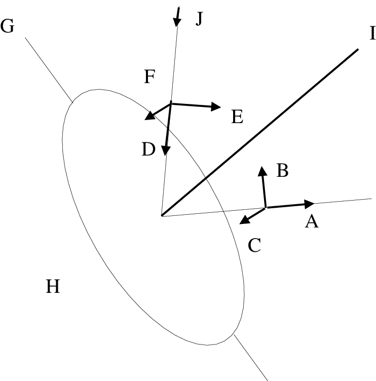
The RF for the incoming beam () is defined by in the propagation direction, in the incidence plane of mirror normal , orthogonal to , and pointing to the mirror normal. is orthogonal on both, forming a right-handed RF. The RF of the reflected beam is constructed analogously from the respective directions. Note that and are identical and parallel to the mirror surface.
The following discussion will concentrate on the more general optical thin aluminium coatings1919 19 i.e., the value of the thickness of the coating . The corresponding formulation for optically thick coatings can be found in Appendix C.
The mirror matrix M in this case is given by2020 20 Jaeger Oetken, [10]
| (5.10) |
The conventions used are2121
21
Almost literally from Skumanich et
al., [24], p.379f.:
(1) The electromagnetic wave is described by .
(2) The components are defined in the canonical RF / RF′
as given above.
(3) The reflectivities are defined by = .
(4) The given values are the incidence angle, , the
refractive index, , the absorption coefficient, , the thickness of
the mirror coating in wavelength fractions, , and the
refractive index, , of the substrate below the coating.
Under this conditions the matrix entries can be calculated by the following
equations2222
22
The equation were also taken from [24],
p. 380. A derivation is possible from Born Wolf, Principle of
optics, [2], chapters 1.5, 13.2, and 13.4.:
| (5.11) |
where
| (5.12) |
and
Taking and with real , the entries of the matrix are
| (5.13) | |||||
For optical thick coatings the substrate below the coating can be neglected, and the equations simplify (see Appendix C).
It is assumed, that a sufficient polarimetric accuracy of the telescope model
can be achieved also with the simplier equations (M.Collados, personal
note). The resulting values for the refraction indices would in that
case have to be interpreted more as effective than as physical
values. Both sets of equations will be used to check the consistency. If
the coating thickness is used as free parameter in a
least-square-fit to telescope calibration data, its value should allow
the decision, which equations are best suited to describe the telescope.
Summary:
The Mueller matrices of the single mirrors have to be calculated for
each point in time with the momentaneous incidence angles, while the
other parameters entering are constant physical mirror properties.
Rotation matrices
To transform between different RFs, in general a base
transformation has to be performed. This is simplified by the fact
that the beam directions of subsequent optical elements are identical, i.e. for
example the reflected beam of C1 ( from Fig. 5.4) is the incoming
beam of C2 ( of C2).
Only the axes orthogonal to the beam direction can be different and the
transformation can be established by a rotation around the -axis.
The matrix of a rotation is given in Appendix A.6.
The only thing to be considered additionally is the direction of the
rotation: the rotation angles are to be measured by convention
counter-clockwise from to , when looking towards the light
source. The primed vector is from the RF to be transformed
to2323
23
Capitani et al., [3], p. 177. Neglection of the
convention can easily lead to sign errors in the calculated angles,
which are very difficult to track down.
Window matrix
The windows of the vacuum tank can exhibit stress induced
birefringence. The entrance window is modellized as pure retarder with
an arbitrary, but fixed, position angle of the fast and slow
axis2424
24
As in Skumanich et al., [24], p.362 .. Its
properties can be included by the two parameters retardance, ,
and position angle, . The exit window is assumed too small to
show polarizing effects at all. Values for the parameters result from the least
square fit to the telescope calibration data.
The paper of Owner-Petersen, [17], gives a derivation for this modellization. If the telescope model is seen to give an unsufficient fit, a more rigid approach for the entrance window will be tried following the considerations in the paper. Additionally the possibility to exclude the window will be investigated. Then the main effect caused by the window, an increased retardance, should be included in the effective physical values of the main and deflection mirror. The way of treatment in this case is still an open issue, depending on actual measurements at Tenerife.
5.2.1.3 Additional reference frames
In addition to the RFs of the single mirrors, which are defined by the beam path and the mirror normals, three other RFs are needed. The first is a RF, which stays fixed on the sun. Into this RF the measurement result has to be transformed at the end. The second one is the actual measurement RF of the polarimeter, while the third one is the coordinate RF (’main RF’) for all following calculations of vectors.
- •
The main RF has its origin in the center of the first mirror C1 and is defined by:
Its orientation can be seen by moving the coordinate directions in Fig. 5.3 from the center of the entrance window to the center of C1. Four different ways are used later to describe a vector in the main RF :
- (1)
Horizontal plane coordinates: the horizontal angular height, , equal to 90∘ - zenith distance, and the azimuth, , given by the angular distance between S and the projection of the vector to the x-y-plane, increasing from S to W2525 25 H.-H. Voigt, Abriss der Astronomie, [28], p.1f.
- (2)
Equatorial coordinates: declination, , the angular distance from the equatorial plane. This plane is inclined by (90∘ - geographical latitude) to the horizontal plane. The second coordinate is the hour angle, , in the equatorial plane, which also is increasing from S to W. This is not identical to the azimuth because of the angle between these two planes2626 26 Voigt, [28], p.2.
- (3)
Spherical coordinates: , the angle to the -axis (equal to zenith distance), and , the angle in the --plane, this time increasing from to , i.e. from S to E, therefore equal to .
- (4)
Cartesian coordinates and as given by the definition of the axes.
Transformations between these coordinate systems are:
- –
for 2727 27 Voigt, [28], p.5:
(5.14) (5.15) (5.16) - –
for :
(5.17) - –
for :
(5.18)
- (1)
- •
For the solar RF it is sufficient to fix one axis. This reference axis is the tangent to the equatorial plane at the hour angle of the sun. If this vector is moved in angular height to the sun center, it bisects the sun from W to E. This direction is given in the cartesian main RF by
(5.19) where denotes the geographical latitude and the hour angle.
- •
The measurement RF of the polarimeter is defined through the zero position of the transmission axis of the linear polarizer of the calibration unit as . The rotation between telescope and polarimeter at the end of the optical train will be used as free parameter, to compensate errors in the initial positioning of the calibration unit.
5.2.1.4 Calculation of the telescope matrix
To calculate the polarimetric properties of the complete telescope, consisting of the four mirrors C1, C2, main and deflection mirror, and the entrance window of the vacuum tank, the following parameters2828 28 Remark: for optically thin coatings. are needed:
- •
mirror properties : refraction index, , absorption coefficient, , thickness of the aluminium coating in wavelength fractions, , refraction index of substrate,
- •
window properties : retardance, , position angle, ,
which are constant properties of the system, and
- •
position angle of C1 on the circle of rails (azimuth)
- •
sun position,
which define the beam path.
With the last two parameters the path of the light beam in the telescope
can be constructed, also the mirror normals and the RFs of the single
mirrors. This gives the values needed for the calculation of the Mueller
matrices of the optical train, namely
- •
incidence angles on the mirrors :
- •
rotation angles between RFs : .
The actually used input parameters of the routine are the constant physical properties, which will be stored in a separate file, and the azimuth of the first mirror, date, and time of the measurement.
The construction of the beam path
The beam path is defined by three direction vectors, corresponding to the bold arrows in Fig. 5.5 :
- •
- •
The position of the second mirror C2 as seen from the center of C1.

Figure 5.5: (top) The position of the second coelostat mirror C2 relative to C1. The origin lies in the center of C1. The position angle in the horizontal plane is fixed by the azimuth of the first mirror. The mirror normal on C1, , is in the equatorial plane, which is inclined 90 to the horizontal plane. Bold arrows denote the beam path. The declination of the sun is negative. The entrance window would be vertically below C2.
The declination of the second mirror, , is the negative of the declination of the sun, , as the (bottom) part displays. There the line with the arrows connects the centers of the sun and the second mirror. From the law of reflection it follows, that it is exactly bisected by the mirror normal , and is orthogonal to it. The triangles built by the footpoints in the equatorial plane, the intersection point and the positions of sun or C2 are identical, therefore .The coordinates of C2 are -unfortunately in two different coordinate systems- given by
declination in equ. plane coordinates azimuth in hor. plane coordinates The first stems from the fact that the mirror normal on the first mirror, , always is in the equatorial plane. Due to the law of reflection C2 then must have the value opposite to the sun with regard to the equatorial plane (see the lower part of Fig. 5.5). The second coordinate, , can easily be derived from the definition of the azimuth in section 5.2.1.1.
The value, which needs to be established here, is the horizontal height, . To solve the equations (5.14)-(5.16) in this case a numerical solution is used. Multiplication of Eq. (5.15) with and of Eq. (5.16) with , and addition of the modified equations gives:
(5.20) with the known values and , the only unknown parameter is the angular height .
- •
The vertical beam path after C2. This direction simply is (0,0,-1) in the main RF.
The mirror normals
The direction of the mirror normal on C2 is easy to construct. The incoming beam has the direction , the reflected beam must be vertically downwards. The mirror normal therefore has to be inbetween - and (0,0,-1). As these directions have the same length (both are normalized), the mirror normal is given by2929 29 A proof is simple, this follows from the properties of an isosceles triangle.:
| (5.21) |
The mirror normal of C1, , is constructed in the same way from and :
| (5.22) |
The incidence angles
The incidence angles on the respective mirrors can be calculated from the standard scalar product, , between mirror normal and the direction of the incoming or reflected beam. So each can be calculated in two ways3030 30 For control one can calculate , which is also valid.:
| (5.23) | |||||
| (5.24) |
The incidence angles on main and deflection mirror are constant with , which can be derived from Fig. 5.3.
Construction of the reference frames
The RFs of the single mirrors are determined by beam directions and mirror normals. An example will be executed for an incoming beam (see Fig. 5.6).
The axis , equal to the inverse direction of the incoming beam, the mirror normal and the x-axis lie in the same plane (incidence plane). The two vectors and are an ONB for every vector in the incidence plane, thus can be decomposed by
| (5.25) |
where .
With
| (5.26) |

The mirror normal can be decomposed into two orthogonal parts. One is parallel to the propagation direction, . It is given by .
The other, , is parallel to the unknown x-axis in the incidence plane. The x-axis direction can be calculated by normalizing .
a direction is obtained, which is orthogonal to the propagation direction, points from it to the mirror normal, and lies in the incidence plane, the requirements for the x-axis in section 5.2.1.2.
The y-axis can be calculated by:
| (5.27) |
where denotes the standard vector crossproduct.
Calculation of the rotation angles
Two different subsequent RFs have one axis in common, that is the propagation direction, . One needs to establish the rotation angle around this axis, arbitrarily oriented in space, that moves onto its counterpart . This can be done numerically for the calculated unit vectors of the RFs, which shall not be disussed in detail3131 31 The condition of counter-clockwise rotation unfortunately excludes the use of the scalar product..
The final matrix product
5.2.2 Telescope calibration data
The principle of the telescope calibration is identical to the
polarimeter calibration. It consist of the creation of known input
Stokes vectors, and the measurement of the corresponding polarimeter
output. After the application of the inverse of the X-matrix the
properties of the polarimeter can be assumed to be removed from the
data. The difference is the time dependence of the T-matrix,
which makes a fit of constant matrix entries like for the polarimeter
impossible.
The main problem of the telescope calibration unit is the size needed. It has
to cover the full area of the first coelostat mirror or the entrance
window. This can not be achieved with a single sheet polarizer of
sufficient quality. Large sheet polarizers are subject to spatial
inhomogeneties due to deformations of the surface. The telescope
calibration unit therefore consists of an array of sheet polarizers. The
single sheets are placed in separate mountings and can be aligned
individually. The whole array is rotateable to create different linear
polarizations (see Fig. 5.7). Unfortunately the
calibration unit is too heavy to be placed freely in the beam path above
the first mirror3232
32
This would additionally require a larger
covered area, and an accurrate co-motion with the mirror.. The possible
positions of the calibration unit are on top of the first mirror, which
also solves the problem of accurate co-motion to guarantee an input
constant in time, and on top of the entrance window after the coelostat
mirrors.

The covered area corresponds to the diameter of the first mirror. The 19 quadratic sheet polarizers can be separately aligned. The array can be rotated as a whole to create different linear polarizations. It can be placed either on top of the first coelostat mirror C1 (Fig. 5.10) or on the entrance window (Fig. 5.8).
The telescope calibration unit thus allow two different sets of data to be created. Each set will consist of a full (half) revolution of the calibration unit with a stepsize of 10∘ (5∘). The data sets include different optical elements of the telescope and will have to be evaluated in correct order, but not fully separetely.
5.2.2.1 Calibration unit on top of the entrance window

Fig. 5.8 shows the corresponding telescope calibration unit
of the TIP with polarizer sheets in the infrared wavlength range on
that position.


The array of polarizers is placed on top of the entrance window and rotated for an angle in already polarized light. The resulting matrix is applied on unpolarized sunlight with the intensity . The transmitted intensity is given in of the incident intensity. See text for more details.
If the telescope calibration unit is placed on top of the entrance window, the optical elements below are the entrance window, the main and the deflection mirror. The zero position of the polarizer is the W direction (= of the main mirror RF), the array has to be rotated from W to N to give a counter-clockwise rotation.
Both mirrors are usually coated at the same time. Their polarimetric properties can be assumed to be identical, and should exhibit only small changes on longer time scales due to their evacuated environment.
With the inclusion of the entrance window as optical element and using the description of optical thin mirrors (see section 5.2.1.2 above) the following parameters are open in the reduced model:
- •
for the mirrors. The label ’vac’ indicates that these values are supposed to be valid only for the mirrors in the vacuum tank.
- •
for the entrance window.
- •
between telescope and polarimeter.
Even if it seems that the coelostat mirrors can be neglected for this part, they still have an influence. The polarizer array is rotated in already polarized light. This leads to intensity variations like already discussed in section 5.1. The equation connecting input and output is:
| (5.30) |
is the restriction of the telescope model on the elements after the polarizer. The time dependence of takes into account small variations in total intensity and the polarization content resulting from the motion of the first coelostat mirror. The values of and , i.e. the polarization introduced by the coelostat mirrors, are of order of some . If the polarizer now is rotated, the intensity in may vary by the same amount, with the total intensity also unknown. The intensity variation can be seen in Stokes I in Fig. 5.9. The macxima and minima in the curve occur, if the polarizer is aligned parallel or anti-parallel to the linear polarization produced by the two coelostat mirrors. For an azimuth of C1 the order of the intensity variations increases strongly.
To remove this intensity variation the following procedure may be used3333 33 Keeping the polarizer fixed as for the polarimeter calibration data is no option here. The left side of eq. (5.30) is normalized with the intensity after the application of the inverse X-matrix:
| (5.31) |
where and is the polarization information.
The right side is constructed from an unit intensity input, and the final input vector is also normalized:
| (5.32) |
This should allow to perform a least square fit of the free parameters , and . The intensity information lost by the normalization is not needed for the fit of the model parameters, as the T-matrix is intensity normalized anyway, i.e. divided by . See the discussion on additional intensity variations due to geometrical effects in the following section.
5.2.2.2 On top of the mirror C1

In this case the light passes the polarizer twice. After the second
tranmission through the calibration unit the beam path includes all
remaining elements in the telescope model. The properties of the
entrance window and the subsequent mirrors can assumed to be known. The
open parameters now are , and , where the
label ’coel’ refers to the two coelostat mirrrors only. The thickness of
coating may be dropped for optical thick coatings, see the discussion in
5.2.1.2.
This seems to be easy to achieve, but the setup causes a mayor
problem. The polarizers of the calibration unit are assumed to be ideal,
and they are passed again after the first mirror. The only way to retain
the information on the properties of this mirror is to use here a
non-normalized T-matrix, contrary to the section above and the
application on observational data. It seems necessary to explicitly
derive how the information is still available, even with an ideal
polarizer.
To simplify the calculation a ’quasi-ideal’3434 34 ’ideal’ would additionally require . mirror, i.e. the assumption of a retardance of in eq. (5.10), is used. Its Mueller matrix is:
| (5.33) |
where , and .
If the optical train for the rotated polarizer with the angle before and 3535 35 The minus arises due to the counter-clockwise definition of the angle. The x-axis of the mirror is assumed to coincide with the zero position of the array of polarizers. after the mirror is calculated, the transmitted intensity is:
| (5.34) |
For the intensity I is constant. In all other cases a
modulation of the intensity dependent on the mirror properties remains.
It should thus be possible to extract the properties of the first coelostat mirror from the intensity I in the data set. Fig. 5.11 displays a result for eq. (5.34) predicted from the telescope model.


The array of polarizers is placed on top of C1 and rotated for an angle . The resulting matrix is applied on unpolarized sunlight with the intensity . The transmitted intensity is given in of the incident intensity. See text for more details.
The non-normalized matrix with the inclusion of
the polarizer array on C1 is applied on unpolarized sunlight with the
intensity . The physical mirror paramters were taken from an
ASP telescope calibration and can be found in the caption. The variables in
eq. (5.34) here are and
, calculated from
eqs. (5.11)-(5.13)3636
36
The calculated retardance of the
first mirror is , which motivates the neglection of the
off-diagonal terms in the lower right corner of
the mirror matrix.. The total transmitted intensity drops to about 16
of the incident intensity, which will require longer integration
times. Note that the position of the extrema in Stokes I (=extrema of
eq. (5.34)) are not directly related to the extrema of the polarizations
(dependent on angle ).
From observational data taken with a calibration unit of similar design in the infrared range (see Fig. 5.10) an additional complication seems to be present. The array of polarizers does not cover the full area of the mirror. There are strong hints that in the rotation of the array an intensity modulation appears due to a cross-mounting holding a folding mirror in the vacuum tank. This mirror reflects light out of the beam path to the telescope guiding system. A rotation of the structure of Fig. 5.7 over this cross-like pattern of non-neglectible extension leads to a variation in intensity of an order similar to the one due to eq. (5.34). It may be necessary to remove this purely geometrical effect by a calculation of the area shaded for each angle to obtain the information important for the polarimetric properties.
5.2.2.3 Additional possibilities for the telescope calibration
There are some other methods to establish the instrumental polarization of the telescope. They mainly differ in the way used to create the known polarization input of the incoming beam.
- •
The usage of the presumably unpolarized sun light from a non-magnetic region at disc center, corresponding to a Stokes vector of (I,0,0,0). This has some disadvantages:
- –
The application of the telescope matrix on unpolarized light only uses the first column. No direct control of the entries of the cross-talk between polarization states is possible.
- –
The window properties will most likely not be well determined, as they are more important for the polarized states than intensity.
This input of unpolarized light should only be used in addition to other data in the determination of the instrumental polarization, but is well suited as a control value for predictions of the telescope model.
- –
- •
The usage of a sunspot with a magnetic field aligned parallel to the LOS. The magnetic field lines are assumed to be vertically upwards, with regard to the solar surface, in the center of the umbra of a sunspot. Depending on the position of the spot on the solar disk a point may contain field lines parallel to the LOS. The emerging light of this point then is polarized only circularly, corresponding to a Stokes vector of (I,0,0,V). This has the only drawback to find a suited sunspot near disk center at the day of the calibration measurements. As this coincidence can not be planned, this possibility should also be seen as an addition.
- •
The usage of mirror parameters measured in a laboratory from samples. These samples always must be kept under the same environment conditions as the telescope mirrors. This method seems to have too many error sources to be used. The results for the mirror parameters at the Dunn VTT strongly deviate from literature values for aluminium coatings, which were measured in optical laboratories. The mirrors are part of a complicated optical setup, where not all polarization-sensitive elements in the beam path may have been explicitly included in the telescope model. Most likely this will lead to effective values for the physical parameters only weakly connected to, for example, the actual refraction index of a single mirror.
Chapter 6 Observations with the ASP: evaluation of polarimetric data
”Forget about the ASP for a moment…”
M.Collados Vera (2002, in a discussion)
The evaluation of two data sets from the ASP was performed prior to the
diploma thesis as preparation to the calibration of POLIS. It was
intended as a preliminary examination of the quality of the data, and to
get used to polametric data. All interpretations and conclusions drawn
stem from the limited knowledge of the author on the discussed
subjects11
1
And may be wrong.. Again here actual data from POLIS
was planned to be used, but this was impossible due to the delayed setup.
The section shall demonstrate the properties and some evaluation possibilities of polarimetric data. Some of the effects mentioned in section 2.1 can be displayed.
6.1 Measurement data: size and content
The data sets available were a scan of 239 scan steps over a magnetic active region with emergent flux, and a single sunspot with 120 scan steps.

In Stokes I four spectral lines can be identified. The sharp lines at 630.20 nm and 630.27 nm are telluric -lines formed in the atmosphere of the earth. They can be used for a calibration of velocities, as they show no systematic Dopplershift due to any systematic motion. The two FeI lines at 630.15 and 630.25 nm are of solar origin. The line with the greater Landé factor shows a visible splitting.
The linear polarizations Q and U correspond to the case depicted in Fig. 2.4, bottom right.
The observation direction is not perpendicular to the magnetic field, so also a vertical component is present as proven by the signal in Stokes V. These profiles were taken from the data set of an active region and show a great amount of linear polarization, while in the sun spot data set the magnetic field is mainly vertical.
The polarimetric data measured by the ASP is the intensity and the polarization content for the wavelength range from about 630.0 nm to 630.4 nm (cp. table 4.1). Fig. 6.1 gives the profiles in one row of a data image from the active region. There are four spectral lines included in the intensity spectrum of Stokes I:
- •
two telluric -lines, which are formed in the atmosphere of the earth at their rest wavelength. They can be used as reference for absolute velocity calibrations or to measure the spectral dispersion per detector pixel.
- •
two FeI lines of solar origin. These may show Dopplershifts due to relative motions, between earth and sun, the solar rotation and finally motions of material in the photosphere of the sun. The displacement from their rest wavelength gives the LOS velocity. In the profiles of Fig. 6.1 the magnetic field strength is sufficient to produce a visible splitting of the line with the greater Landé factor in the intensity profile. The intensities of the linear polarizations Stokes Q and U give information on the horizontal field component, while the signal in Stokes V is proportional to the LOS component.
More information on the spectral lines can be found in table 4.4. Along the slit height corresponding to 74 arcsecs on the solar image 229 rows of (I,Q,U,V) profiles are available for each scan step. A reduction to two-dimensional maps of selected parameters is shown in for example Fig. 6.6 and 2.2.
6.2 Evaluation of the Stokes V signal

The amplitudes can be used for the construction of magnetograms. The positions of minmum and maximum exchange when the magnetic field lines are of oppposite direction. Subtraction of the areas under the single peaks, , gives the net circular polarization (NCP). The wavelength of the zero-crossing, , is the position of the -component, which is not influenced by the magnetic field. The calculation of the zero-crossing velocity from gives the velocity of material inside the magnetic field. This can be compared to the velocity derived from the intensity profile, containing mostly the non-magnetic environment.
An accurate measurement is easiest for the Stokes V signal for two reasons:
the magnetic fields on the sun are usually more vertical than horizontal with
regard to the solar surface, thus they are more or less oriented
parallel to the LOS. Therefore the signal in V is usually the
strongest. Secondly, the polarization effects of mirrors or other
optical devices in the beam path are smaller for circular
polarization. Before the use of vector polarimeters so-called
magnetographs (cp. the introduction to chapter 3) were
mainly in operation for solar magnetometry, which measure the amount of
circular polarization only.
Fig. 6.2 gives an idealized Stokes V profile for a magnetic sensitive spectral line. It is useful to define the following quantities for an evaluation:
- •
are the maximal amplitudes of the signal at the position of the left or right circular component. A magnetic field with the oppposite direction exchanges the position of the peaks, i.e. then the minimum would preceed. The amplitude can be used for the construction of magnetograms like in Fig. (6.6) or (2.2). They give an estimation of vertical strength and the direction, sometimes called polarity, of the field.
- •
is the area under the single peaks. Their subtraction results in the net circular polarization (NCP).
- •
The zero-crossing wavelength is the position of the transition (-component) of the spectral triplet, that is not influenced by the magnetic field (cp. Fig. 2.3).
6.2.1 The zero-crossing velocity
The last item, the zero-crossing wavelength, is important to establish the LOS velocity of material in the magnetic field, . This may be different to the velocity derived from the intensity line profile, which contains contributions from non-magnetic areas. Examples of velocity maps are displayed in Fig. 6.3 for the sunspot data. The pattern of velocities towards and away from the observer, roughly anti-symmetric to the direction to the center of the solar disk (not drawn), is caused by the Evershed effect. This is assumed to be a radial outflow from the sunspot center, where the different viewing angle on the spot changes the measured LOS velocity22 2 see Westendorp et al. (2001), [29], or Schlichenmaier and Schmidt (2000, [20] and [21]) for a detailed examination of LOS-velocities in a sunspot.


Outside the spot single granulation cells can be identified, in which hot material is rising, then cooling and sinking down at their borders. The anti-symmetrical pattern of motions towards (lower hemisphere) and away from the observer (upper hemisphere) in the spot is caused by the Evershed effect. The radial outflow of material from the spot center has an effective LOS component depending on the azimuthal position in the spot. For the area in the central umbra, where the line profile splits up, the evaluation method with a parabola fit is not suited, as the artifacts in the left panel display. The zerocrossing map of the velocity in the magnetic field shows the same general structure. Here the central umbra with strong Stokes V signals presents no difficulties for the calculation of the zero-crossing wavelength. In the uniform black area outside the spot no zero-crossing can be established (insufficient V signal). The magnetic field extends over the boundary of the penumbra in the continuum (outer white line). The limit for the evaluation of a Stokes V profile was a minimal polarization content of 1 , which is exceeded in the outer regions as well.
The diagnostic importance of the zero-crossing velocity is shown in Fig. 6.4. The difference between the LOS velocity from the intensity profile, , and displays some features:
- •
Single magnetic elements outside the spot may show up as well as down flows relative to their environment.
- •
The Evershed effect can still be seen in the two images, which give the difference of the velocities, , for and separately. Above the spot the filling factor, i.e. the fraction of area covered by magnetic fields, can assumed to be 100 . Therefore no velocity differences should be seen at all, as all material is inside magnetic fields. Single unresolved, concentrated magnetic structures with a small filling factor inside a detector element would contribute to the Stokes V signal, but only little to the intensity due to the small area covered. If these structures have a significantly differing mass velocity, they may cause an additional shift of the zero-crossing wavelength relative to the intensity line core. The clearly visible remaining velocity differences therefore hint to unresolved magnetic elements in the penumbra.
- •
The rectangle in the left image highlights a substructure inside the penumbra. In an extension of a brightening in the continuum intensity a radially oriented region shows to be greater than the doppler velocity by about 1 km/s. Such a feature can be explained by the model of single flux tubes embedded in the background field of a sun spot (Schlichenmaier, [19], 1997). This model predicts nearly horizontal flux tubes in the outer penumbra, inside which flows of up to 15 km/s can appear. If one assumes the remaining velocity difference to be caused by a horizontal flow in a single flux tube, and a viewing angle of about 10∘, the horizontal speed would need to be here app. 6 km/s greater than in its environment.


Outside the spot the velocity in isolated magnetic elements shows up as well as down flows relative to the non-magnetic environment. The Evershed effect remains even after the subtraction of both images. The white rectangle marks a feature in the outer penumbra, where in an extension of a brightening in the intensity a radial oriented region with a velocity difference of about 1 km/s can be seen.
6.2.2 Net circular polarization
The area under the single wings of the Stokes V profile, and , should be equal for a static atmosphere in local thermal equilibrium. Fig. 6.5 displays, that this is very often not the case in the sunspot. In the upper hemisphere the complete penumbra shows net circular polarization (NCP), i.e. an integration along the wavelength dimension leads to a residual value not equal to zero. The NCP value changes abruptly at the border of penumbra and umbra from the continuum image, in difference to the magnetogram, where the transition is smooth. This behaviour can be also be explained by the model of moving flux tubes on the background field of the sunspot (Schlichenmaier, [19], 1997, and Schlichenmaier et al., 1998). The existence of more horizontal, isolated flux tubes in the outer penumbra, in which the plasma moves radially outwards with a speed of about 15 km/s, leads to gradients in either the velocity and the magnetic field strength along the LOS. If gradients in both environment parameters are present, the produced Stokes V signal has a non-vanishing NCP. Inside the umbra no isolated elements appear.
The particular shape of the NCP, being roughly symmetric to an axis from the top to the bottom of the image, is predicted by the thesis of Müller, [16], 2001. In this thesis synthetic NCP maps of axialsymmetric sunspots for different spectral lines were examined, which were constructed by placing the final results of the moving tube simulations into a three-dimensional background field. The calculation of the NCP of the Stokes V profile along the LOS around the spot resulted in a symmetric shape for the iron line at 630.25 nm. For another iron line at 1564 nm the NCP should be anti-symmetric. This could be confirmed by observations with the Tenerife Infrared Polarimeter (TIP) (Schlichenmaier et al., 2001).

The NCP gives the difference between the areas and , if the V signal is zero outside the magnetic sensitive spectral line. If the NCP is not equal to zero for the whole profile, the Stokes V signal is not fully anti-symmetric. The NCP apruptly changes at the border bewtween umbra and penumbra in the upper hemisphere. This indicates quite different environment conditions, mostly in material velocities, as the magnetogram in Fig. 2.2 shows a smooth transition.
To give one additional example of polarimetric data, Fig. 6.6
shows some maps of the other data set taken with the ASP. This active
region is dominated by the increased appearance of opposite
polarities, i.e. magnetic fields with opposite directions, opposite to
the sun spot data with mainly a single polarity. A time series
was taken for the area in the center of the image, where the dopplergram
shows the disturbation of the granulation pattern by the magnetic
fields, to study the evolution of this emerging magnetic flux. A
complete evaluation of the data set requires an inversion. An extended
discussion of the data can be found in the report on the
’Hauptpraktikum’,[1].
Summary:
Polarimetric data of the Stokes vector allows to calculate the
vector magnetic field, i.e. field strength and direction. The
zero-crossing wavelength gives the velocity of material inside magnetic
elements, which may differ from the Doppler velocity of the intensity
profile. The NCP hints to gradients in velocity and field strength. It
can be used to test theoretical models. The environment conditions in
umbra and penumbra of sunspots are different. Last, but not least: every
interpretation of polarimetric data rests on the assumption, that the
effects are of solar origin only. The calibration of the data should be
better than the order of the observed effect, especially for the correct
interpretation of weak polarization signals.


The signed amplitude of the Stokes-V signal in of the mean intensity with superimposed borders of the umbra and penumbra.
The amplitude is proportional to the magnetic field strength, while its sign distinguishes the field direction to or away from the observer. Some of the pores and the sunspot at the left border of the area can be seen to be of opposite polarities. The region in the center of the image shows additional magnetic activity, which is not visible in the continuum intensity above.

A Dopplergramm of the LOS velocities relative to the solar surface with superimposed borders of the umbra and penumbra.
The velocity pattern outside the strong magnetic fields reflects the movements of the granulation, hot material rising and cooler sinking. The Evershed flow can be seen in the greater sunspot. The granulation pattern between the two spots is slightly distorted, presumably due to the presence of magnetic field in that area.
 A logarithmic map displaying .
The Stokes parameter Q measures linear polarization,
which corresponds to more horizontal magnetic fields. These are
strongest in the area between the two pores of different polarity at the
left border. This can be explained by field lines connecting the
oppposite polarities in a loop, where at the top of the loop the field is
horizontal. The cross-like structure in the greater sunspot is caused by
the axialsymmetric field of a spot, where the angle between
LOS and magnetic field lines is the same for different positions around
the spot center.
A logarithmic map displaying .
The Stokes parameter Q measures linear polarization,
which corresponds to more horizontal magnetic fields. These are
strongest in the area between the two pores of different polarity at the
left border. This can be explained by field lines connecting the
oppposite polarities in a loop, where at the top of the loop the field is
horizontal. The cross-like structure in the greater sunspot is caused by
the axialsymmetric field of a spot, where the angle between
LOS and magnetic field lines is the same for different positions around
the spot center.
The continuum intensity drops to 25 of the maximum intensity in the sunspots and pores. The spot itself can be divided in dark umbra and brighter penumbra. In comparison with Fig. 2.2 the minimal intensity is higher, while the Stokes-V amplitude is lower.
Bibliography
- [1]
C. Beck , Kalibration und Auswertung von
ASP-Daten (Hauptpraktikumsbericht), April 2001, KIS library, in german
The report on the ’Hauptpraktikum’ gives a slightly shortened translation into german of the theory as described in [4]. Further the calibration of an ASP data set is discussed as well as results of a preliminary evaluation. - [2] M. Born, E. Wolf , The Principles of optics , Pergamon, New York, 1970
- [3]
C. Capitani, E. Landi degl’Innocenti,
F. Cavallini, G. Ceppatelli, M. Landi degl’Innocenti , Polarization properties of a ’Zeiss-type’ coelostat - The case of the
solar Tower in Arcetri , Solar Physics, vol. 120, no. 1, 1989,
p. 173-191
A theoretical description of the polarizing properties of a ’Zeiss-type’ coelostat which can be transferred on other coelostats as well by considering the different geometrical design. - [4]
Edward Collett , Polarized light :
fundamentals and applications , Marcel Dekker Inc., New York, 1993
The book of Collett gives a very extensive derivation of the Stokes and Mueller calculus and also other theoretical descriptions of polarized light. Its primary strong point are the many examples used to demonstrate the theory and the interesting remarks on the historical evolution in this field. - [5] W. Demtröder , Band 3 : Atome, Moleküle und Festkörper , Springer, Berlin, 1994
- [6]
D.F. Elmore, B.W. Lites, S. Tomczyk,
A.P. Skumanich, R.B. Dunn†, J.A. Schuenke, K.V. Streander,
T.W. Leach, C.W. Chambellan, H.K. Hull, L.B. Lacey† , The Advanced Stokes Polarimeter : A new instrument for solar magnetic
field research , AAS, 1992
A full description of the ASP dual beam polarimeter, only the part about the nonlinearity of the cameras has become obsolete. - [7] G.E. Hale , On the probable existence of a magnetic field in sun-spots , ApJ 28 , 1908
- [8] U. Grossmann-Doerth , Height of formation of solar photospheric spectral lines , Astron. Astrophys., 285, p. 1012-1018, 1994
- [9] U. Grossmann-Doerth, B. Larsson, S.K. Solanki , Contribution and response functions for Stokes line profiles formed in a magnetic field , Astron. Astrophys., 204, p. 266-274, 1988
- [10] F.W. Jaeger, L. Oetken , Zur Theorie und Praxis der instrumentellen Polarisation I II , Publ. des Astrophys. Observatoriums Potsdam, Band 31, Nr. 103 107, Akademie-Verlag Berlin, 1963 1968
- [11] A. Kuc̆era, H. Balthasar, J. Rybák, H. Wöhl , Heights of formation of Fe I phostospheric lines , Astron. Astrophysics, 332, p. 1069-1074, 1998
- [12] E. Landi Degl’Innocenti , Magnetic field measurements , in: Solar Obseravtions: techniques and interpretation, Sánchez, Collados, Vázquez (Eds.), Cambridge Univ. Press, 1992
- [13]
B.W. Lites , Rotating waveplates as
polarization modulators for Stokes polarimetry of the sun : evaluation
of seeing-induced crosstalk errors , Applied Optics 26 , 3838,
1987
Also includes details on the demodulation scheme. - [14] P. Magain , Contribution functions and the depths of formation of spectral lines , Astron. Astrophys., 163, p. 135-139, 1986
- [15] Mayer-Kuckuck , Atomphysik , Teubner, Stuttgart, 1997, 5.Auflage
- [16] D. Müller , Polarisation von Linien im Spektrum einer Sonnenflecken-Penumbra (Dipl. thesis) , Freiburg, 2001
- [17] M. Owner-Petersen , On the polarization effects of stress induced birefringence of the entrance window of solar telescopes , LEST Foundation, Technical report No. 49, 1991
- [18] J. Sánchez Almeida, B. Ruiz Cobo, J.C. del Toro Iniesta , Heights of formation for measurements of atmospheric parameters , Astron. Astrophys. 314, p. 295-302, 1996
- [19] R. Schlichenmaier , Die Dynamik magnetischer Flußröhren im Sonnenfleck (Diss.) , LMU München, 1997
- [20] R. Schlichenmaier, W. Schmidt , Flow geometry in a sunspot penumbra , Astron. Astrophys. 358, p. 1122-1132, 2000
- [21] W. Schmidt, R. Schlichenmaier , Small-scale flow field in a sunspot penumbra , Astron. Astrophys. 364, p. 829-834, 2000
- [22]
William A. Shurcliff , Polarized light ,
Harvard University Press, 1962
For questions of more technical nature the older book of Shurcliff still can be used, it includes details on the production and classification of polarizers. - [23] M. Sigwarth , Dynamik solarer Magnetfelder (Diss.) , Februar 1999
- [24]
A. Skumanich, B.W. Lites, V. Mártinez Pillet,
P. Seagraves , The calibration of the Advanced Stokes
Polarimeter33
3
Available in a translation into german by the
author
, ApJ Suppl. 110 , 357, 1997
A detailed description of the telescope model, calibration procedure and results of it for the ASP. - [25]
J.O. Stenflo , Solar magnetic fields ,
Kluwer Academic Publishers, 1994
Strongly theoretical inclined book describing mainly the radiation transport equations and ways to a solution. The short experimental chapter is nonetheless sufficient for a quick overview on polarimetry. - [26] M. Stix , The sun , Springer-Verlag, 1989
- [27]
K.G. Strassmeier , Aktive Sterne :
Laboratorien der solaren Astrophysik , Springer-Verlag Wien/New York,
1997
The book uses the sun, whose activities are best known and are described in detail, to mark differences and commons to active stars. It highlights some not understood features of the solar dynamo in comparison with other stars, mainly the dependence on rotation, as stars require certain conditions before getting active at all.
- [28] H.-H. Voigt , Abriss der Astronomie, Bibliographisches Institut, Mannheim, 1969
- [29]
C. Westendorp Plaza, J.C. del Toro Iniesta, B. Ruiz
Cobo, V. Martinez Pillet , Optical tomography of a
sunspot. III. Velocity stratification and the Evershed effect , ApJ,
V 547, 2001
Appendix A The Mueller matrices
In the Stokes formalism the effects of optical active elements can be formulated as matrices M , which are applied on the Stokes vector S as defined in equation (2.8). The matrix elements are determined from the eletrical field components before () and after () the transmission through the element from the equation
| (A.1) |
For this calculations an equivalent definition of the Stokes parameters with complex field amplitudes is very useful. It is given by substituting equation (2.4) with
| (A.2) | |||||
and changing the defintion of the Stokes parameters to
| (A.3) | |||||
An explicit calculation and also the proof of equivalency can be found in [4]. Here shall only the results for the different optical elements being used be presented.
The polarizer
A polarizer is an optical element with a transmission dependent on the oscillation direction of the electrical field and can be described by
with .
Inserting the electrical field amplitudes into equation
(A.1) one obtains the Mueller matrix of a linear polarizer as
| (A.4) |
The retarder
A retarder has different propagation velocities for the two directions (x,y). It changes the relative phase between the field components. Here is
and the Mueller matrix resulting is
| (A.5) |
The rotator
A rotator rotates (as its name says) the field components by a fixed angle . Here is
and the matrix is
| (A.6) |
Rotated optical elements
The Mueller matrix of the rotator is especially important as it also allows one to determine the effects of rotated optical elements, which often occur in optical designs. The rotation can be included by two rotator matrices around the optical element itself by
One example is the rotating retarder used by either the ASP or POLIS :
| (A.7) |
with and . is the retardance of the modulator and the angle between its fast axis and the x-direction, as always counter-clockwise when looking at the light source11 1 I really like that definition..
Polarizing beam splitter
The Mueller matrix of the polarizing beam splitter is22 2 No derivation given.
| (A.8) |
The matrix multiplication with the rotated retarder above, application on a Stokes vector (I,Q,U,V) and the selection of the first vector entry gives the intensities of the two beams labelled + respectively - as
| (A.9) |
on which the measurement scheme relies.
Appendix B Alignment of the polarimeter calibration unit
In the polarimeter calibration unit two elements have to be aligned correctly, i.e. the direction of the transmission axis of the linear polarizer, and the direction of the fast axis of the retarder have to be established. The measurement setup used is shown in Fig. B.1. In addition to the optical elements under examination a second polarizer as analyzer, a light source, and an intensity detector, in this case a photo diode, are needed. The usage of a wavelength filter for 630 nm is optional to increase the resemblance to the conditions of operation in Tenerife. The field stop reduces the stray light.
The optical train consists of an artifical light source, a field stop, a wavelength filter for 630 nm (optional), the polarimeter calibration unit, a second polarizer as analyzer, and a photo diode as intensity detector. The elements of the calibration unit can separately be rotated clockwise, when looking at the light source, for 180∘.

The axis of the polarizer is established with the use of the second polarizer, the analyzer. The method introduced in Fig. B.2 works without any axes known beforehand. Note that all position angles derived may be off by 90∘, i.e. the axes marked on the polarizers may be the blocking instead of the transmission axes, and the retarder may get the slow instead of the fast axis marked. This can be simply cross-checked with a light source of known polarization, for example reflection under the Brewster angle.

(1)

(2)

Now the analyzer is rotated by 180∘ around the vertical axis. This causes its transmission axis to jump by . The polarizer is rotated again for 180∘, resulting in curve (2).
The minmimal intensity now occurs at the angle . The value was established from a least square fit to the intensities for only. The motor seems to have positioning problems around 45∘, but it is the spare unit hopefullly never to be used.
Half the difference between the angles of minimal intensity is the angle to the vertical, . Thus the transmission axis of the polarizer is 16.5∘ off the vertical in the first minimal position, i.e. it is at -23.8∘ for = 0. The analyzer can then also be marked.


Appendix C The analytical telescope model: discussion and comparison
Section 5.2.1 describes a way for the construction of the telescope model that relies on some numerical procedures. The developed procedure can be applied to optical setups other than a coelostat as well, if the beam path is known. For the restriction on the polarimetric properties of a coelostat it is possible to find an analytical solution. Section C.1 presents the formulae of this solution, section C.2 the mirror matrix for optical thick coatings, and section C.3 a discussion on the plausibility of results from the model, and a comparison between the analytical and the numerical method.
C.1 The analytical solution of the telescope model
The paper by Capitani et al, [3], derives analytically the rotation and incidence angles needed for the description of the instrumental polarization of a coelostat. Only the resulting equations for the important parameters will be presented here.
C.1.1 Position of the second coelostat mirror
This is identically to the discussion in section 5.2.1.4. The position of C2 is fixed by its azimuth , and the horizontal angular height, . For the VTT Tenerife this in fact is easier to establish due to the motion of the first mirror C1 on a circle, while for the solar tower in Arcetri described by Capitani the mirror moves on two orthogonal set of rails (Cap., eqs. (13a)-(13d)). This complicates the calculation of the azimuth due to another degree of freedom.
C.1.2 Analytical equations
The equations derived by Capitani, listed in the required order of calculation, now are:
| (C.1) | |||||
| (C.2) | |||||
| (C.3) | |||||
| (C.4) | |||||
| (C.5) | |||||
| (C.6) |
| (C.7) | |||||
| (C.8) | |||||
| (C.9) | |||||
| (C.10) | |||||
| (C.11) | |||||
| (C.12) |
These equations were mainly used to check the results of the numerical routines, but of course they allow the construction of the telescope model by themselves. For the agreement between the two methods see section C.3 below.
C.2 Mirror matrix for optical thick coatings
The mirror matrix for the description of optical thick coatings is in principle identical to eq. 5.10, but the equations for the calculation of the entries simplify. The matrix is:
| (C.13) |
with .
The entries can be calculated with
| (C.14) | |||
| (C.15) |
by
| (C.16) | |||||
| (C.17) |
is the incidence angle on the mirror, and refraction and extinction coefficient. The thickness of the coating and the properties of the substrate do not enter in the calculation.
C.3 Discussion and comparison of model results
The best test of the telescope model is the comparison with actual measurement data from the telescope, but some consistency checks are possible with the model alone.


The polarization content in of Stokes I for 21.03.02 (solid), 21.07.02 (dotted) and 21.01.02 (dash dotted), azimuth . The fourth curve (long dashes) is for 21.07.02, azimuth . The polarization remains well below 10 of the total intensity, but if one moves the first mirror from the zero position, the telescope polarization strongly increases.
- •
image rotation of the coelostat:
If the first mirror C1 is not on the zero azimuth position, the coelostat will perform a rotation of the sun image of(C.18) This can be checked with the model in the following way:
- –
the definition of an angle of the linear polarization by
(C.19) which can be calculated for , and also .
- –
the usage of ideal mirrors, i.e. the mirror matrices are set to diag(1,1,-1,-1). This corresponds to mirror reflectivities of 100 regardless of the oscillation direction of the incoming light and no cross talk terms .
The rotation of the defined polarization axis can be shown by the difference . This has to be compared to the value of predicted by Eq. (C.18). An example is displayed in Fig. C.2 for the date 21.07.02 and an azimuth setting of C1 of 50∘ for 8:00-18:00 UT. The remaining differences between theoretical value and the output from the modellized coelostat are of order of 0.005∘ and arise from the used numerical procedures.

Figure C.2: Image rotation produced by the modellized coelostat in degrees.
Shown is the difference of the angles for the date 21.07.02 and an azimuth setting of C1 of 50∘ for 8:00-18:00 UT (solid line). The dash-dotted line is the prediction of Eq. (C.18) for the rotation angle. The increase of the rotation angle is caused by the changing declination of the sun. - –
- •
comparison with the results in Cap. et al., [3]:
- –
- –
telescope output for unpolarized input: Fig. C.1 displays the Stokes vector, which leaves the telescope optics according to the model for an unpolarized input. Comparing with Cap., [3], Fig. (9 a-c), which show measurements at the Donati Solar tower in Arcetri, one can see a similar range of values for the polarization content.
The long-dashed curve is for an azimuth position of 40∘ on 21.07.02 . The polarization created in the telescope increases, if the first mirror is moved away from the zero azimuth position.


The 16 entries of the telescope matrix resulting from the model are plotted for 8:00-18:00 UT. The azimuth of C1 was always set to 0∘. (solid) 21.03.02, (dotted) 21.07.02, (dash-dotted) 21.01.02 . The matrix entries are either symmetric or antisymmetric to noon. A comparison of absolute values is more difficult, as this depends on the parameter set used for the physical properties of the mirrors. The cross talk between different polarizations has contributions from geometrical effects (image rotation) and the mirror properties.
Appendix D Technical characteristics
D.1 The grating
The optical design of the grating is a combination of an Echelle and a reflective Littrow configuration. As the entrance pupil with the central obscuration of the telescope is imaged onto the grating, the central part of the grating is not illuminated. This area is used for a small folding mirror that feeds the light beam to the collimator (cp. Fig. 4.2). The grating is slightly tilted about a horizontal axis and the imaging mirror is located above the collimator. The final image plane is formed above the grating. The configuration has only small reflection angles and thus a high optical quality across a large field of view.
| Grating | ||
| 79 grooves / mm | blaze angle: 63.4∘ | dispersion: 12 pm/mm @ 400 nm |
| CCD | ||
| 652488 pixels | pixel size | frame rate: max. 40 Hz |
| Modulator | ||
| @ 630 nm | @ 400 nm | zero-order |
| Interference filters | ||
| 5 nm FWHM @ 630 nm | 1 nm FWHM @ 400 nm | |
| Demodulation | ||
| 15 Hz frame rate | synchronized with retarder rotation | |
| Computer control | ||
| PC-based with Windows NT | ||
Appendix E Many thanks to
In no special order:
Wolfgang Schmidt for the topic, the assistance during the work, the
scientific background, etc.
My parents for their unlimited sponsorship all the time
Manolo Collados for his great patience, and a very important visit to
Tenerife
Bruce Lites for his great patience, and the help in the
calibration of the ASP data sets
Michael Sigwarth for exactly the same
Kai Langhans for the introduction into IDL
Thomas Kentischer for the work on POLIS, the opportunity to
smoke inside, and his great patience
Tayeb Aiouaz for a great time, and much fun with negative
pressure
Helmold Schleicher, Jo Bruls for the new calculations of formation
heights - when only asked if the old values were correct
Carsten Baur, Stefan Henninger, Michael Engler for the weekly
’Skatrunde’
Everybode else I forgot
Appendix F Zusammenfassung (in german)
In dieser Arbeit wird die Kalibration des neuen Spektropolarimeters
POLIS beschrieben. Das Gerät resultiert aus einer Kooperation zwischen
dem Kiepenheuer Institut für Sonnenphysik (KIS), Freiburg, und dem
High Altitude Observatory (HAO), Boulder (USA). Es soll am deutschen
Vakuum-Turm-Teleskop (VTT) des KIS in Teneriffa betrieben werden.
Das Gerät bestimmt den Polarisationszustand des Sonnenlichtes in zwei
verschiedenen Wellenlängen- bereichen bei 400 und 630 nm. Zur Messung
wird eine rotierende Verzögerungsplatte verwendet, die den
Polarisationszustand des einfallenden Lichtes moduliert. Durch einen
polarisierenden Strahlteiler wird die modulierte Polarisation in eine
Intensitätsmodulation umgewandelt. Die Demodulation zur Bestimmung des
Stokes-Vektors erfolgt über ein gewichtetes Integrationsschema.
Um eine ausreichende polarimetrische Genauigkeit von 0.1 der Kontinuumsintensität zu erreichen, muss das eigentliche Messgerät kalibriert werden, um seine Antwort auf verschiedene Polarisationszustände festzustellen. Weiterhin muss die instrumentelle Polarisation des Teleskops bestimmt werden, die den Polarisationszustand des einfallenden Sonnenlichtes verändert.
Zur Kalibration des Polarimeters steht eine spezielle Kalibrationseinheit zur Verfügung, die aus einem Linear-Polarisator und einer Verzögerungsplatte besteht. Die Kalibrationseinheit wird sich innerhalb des Vakuumtanks des Teleskop befinden, wo der Strahldurchmesser des Lichtbündels bereits auf einen Durchmesser von 6 cm verringert ist. Mit dieser Einheit lassen sich durch Rotation der beiden optischen Elemente verschiedene bekannte Polarisationszustände erzeugen, die im Kalibrations-Datensatz gemessen werden. Aus einem Vergleich zwischen dem erzeugten Input und dem gemessenen Output lässt sich die Polarimeter-Antwort-Funktion X durch einen Least-Square-Fit bestimmen. Mit dieser 44-Matrix kann man aus dem eigentlichen Messwert den zutreffenden Stokes-Vektor der Polarisation am Ort der Kalibrationseinheit rekonstruieren.
Die vollständige Kalibration erfordert mehrere zusätzliche Datensätze. Um die Detektoreigenschaften der verwendeten CCD-Kameras zu bestimmen, werden Dunkelstrom- und Flatfield-Daten gewonnen. Aus diesen beiden Datensätzen lässt sich die Antwort der einzelnen Detektorpixel auf einfallende Intensität ermitteln. Diese Detektoreigenschaften werden in Gaintables für die jeweiligen Detektorbereiche gespeichert. Der eigentliche Kalibrations-Datensatz zur Bestimmung der Polarimeter-Antwort wird danach mit den Gaintables korrigiert, um die Detektoreigenschaften zu entfernen.
Die korrigierten Daten werden über die Wellenlängen gemittelt, da der polarimetrische Gehalt im Kalibrationsdatensatz konstant sein sollte. Entlang des Spaltes können jedoch durch Verunreinigungen oder räumliche Inhomogenitäten der Kalibrationseinheit Schwankungen auftreten. Deshalb wird die Antwort-Funktion an vier Positionen entlang des Spaltes durch eine Matrix-Inversion des linearen Problems bestimmt.
Um die Eigenschaften der Kalibrationseinheit zu erfassen, werden
zusätzliche freie Parameter verwendet, wie z.B. die tatsächliche
Verzögerung der Wellenplatte. Die Anwendung der inversen
Polarimeter-Antwort-Funktion X-1 auf Messdaten ergibt den
tatsächlichen Stokes-Vektor des Lichtes am Ort der
Kalibrationseinheit.
Der Strahlengang im Teleskop vor der Kalibrationseinheit umfasst vier Spiegel und das Eintrittsfenster des Vakuumtanks. Um die polarimetrischen Eigenschaften dieses komplexen optischen Systems zu bestimmen, werden die einzelnen Komponenten durch Mueller-Matrizen modelliert. Bei den Spiegeln benötigt man die spezifische Geometrie der Reflexion zur Berechnung der Spiegelmatrix. Die Mueller-Matrix des Spiegels ist jeweils nur in speziellen Koordinatensystemen gültig. Zur Berechnung des Gesamtsystems muss man daher sowohl die Spiegelmatrizen als auch die Koordinatentransformationen bestimmen.
Das Eintrittsfenster steht unter grossem Druck und kann deswegen spannungsinduzierte Doppelbrechung zeigen. Es wird als Verzögerungsplatte mit einer beliebigen, aber festen, Ausrichtung der Achse modelliert.
Das Teleskopmodell ergibt die polarimetrischen Eigenschaften des Systems durch Berechnung des jeweiligen Strahlenganges als Funktion folgender Parameter:
- •
Spiegel: Brechungsindex n, Absorptionskoeffizient k. Die beiden Coelostatenspiegel werden als gleich angenommen, ebenso Haupt- und Umlenkspiegel im Vakuumtank (insgesamt 4 Parameter)
- •
Fenster: Verzögerung, Ausrichtung der Achse (2)
- •
Ausrichtung der Kalibrationseinheit: zusätzliche Rotation am Ende des Strahlenganges (1).
Diese 7 Parameter werden aus Teleskop-Kalibrationsdaten bestimmt. Zu diesem Zweck steht eine drehbare Fassung zur Verfügung, in der Linear-Polarisatoren angebracht sind. Die Fassung kann auf dem ersten Coelostatenspiegel oder dem Eintrittsfenster befestigt werden. Durch eine Rotation um 180∘ lassen sich verschiedene linear polarisierte Zustände erzeugen. Der Polarisationszustand nach dem Teleskop wird mit dem kalibrierten Polarimeter bestimmt. Danach werden die Parameter im Teleskopmodell ebenfall mittels eines iterativen Least-Square-Fits an die Messdaten angepasst.
Nach erfolgter Kalibration von Polarimeter und Teleskop lässt sich mittels
| (F.1) |
der Stokes-Vektor des eingefallenen Sonnenlichtes aus dem Messergebnis
bestimmen.
Im letzten Kapitel der vorliegenden Arbeit wird ein Datensatz eines bereits existierenden Vektorpolarimeters untersucht. Selbst bei dieser nur vorläufigen Auswertung lassen sich Phänomene wie der Evershed-Effekt in Sonnenflecken wiederfinden.
Glossary
chromosphere
the chromosphere is blue, until it turns grey at the
borders of reality
convection / convective zone
energy transport mainly by mass movement
corona
the corona is the part of the sun most intensively revered
in Bavaria by such immortal songs as ’Corona Bavariae, deep unter the
stary night…’
differential rotation
the sun as a ball of gas does not behave as a solid
body, so the rotation speed on the surface
is different depending on solar latitude. The values
range from 26 to 30 days on the poles
Doppler effect
The principal effect is a change of frequency if a source
or an observer of radiation are
moving relative to each other along
their line-of-sight (LOS). In solar physics the Doppler
effect is used
to established the material movements on the sun by measuring the
wavelength
of absorption and emission lines, as the
relative movement of earth and sun is known
flux tube
a magnetic flux tube is assumed to be a highly evacuated
bundle of magnetic field lines
held stable against the gas pressure from
outside by the internal magnetic pressure
of the increased magnetic field. The field strength
rises to values of kG
granulation
the convective energy transport in the outer atmosphere
leads to more or less stable convection
cells. The pattern of the
borders of these cells is called the granulation, while a single
cell
is
called a granule. The material is supposed to rise up in the middle and
flow down at the
borders
line
emission : light of a certain wavelength
emitted by an electron transition between
atomic energy levels,
absorption : lowered intensity at a certain
wavelength in a continuum spectrum caused
by absorption and undirected reemission, in the sun the
outer atmosphere produces the
Fraunhofer lines in this way
magnetic
field : the second component of the
electromagnetic field, appearing in the sun on greater
scale in the form of sun spots and smaller flux
tubes, supposed to be produced by
the solar dynamo
loops : loops of magnetic field lines as
suggested mostly in images taken in the
Hα wavelength
reconnection : the annihilation of
magnetic field lines with antiparallel directions,
supposed to take part
on small scales and producing the energy visible in flares or
other short
time features, where a great amount of energy is set free
photosphere
the photosphere is green for the most part, at least
where it’s not red
plasma
ionized atoms lead to a gas of electrons and
ions, which is highly conductive, a situation
prevalent almost everywhere in the sun
polarimetry
in general the measurement of the polarization state of
light. Today polarimetry has a great
number of applications in science
(magnetic fields, saccharimetry, biology,…) and
technics (stress
tests, quality control of surfaces,…). In solar physics one can divide
into
vector polarimetry with measurement of the full Stokes
vector and ’simple’ polarimetry,
using only one polarization state
pore
a small sunspot without any visible penumbra
quiet sun
region on the sun with no solar activity, i.e. no
sunspots or flares, but only the diffuse small
scale magnetic background
radiative core
in the inner regions of the sun the energy is
transported mainly by radiation, whereas after
a small transient zone the outer atmosphere is convective
resolution
spatial : the distance which two for
example intensity features must have at least
on the sun to be detectable seperately
spectral : the minimal distance in
wavelength which can be separated
solar cycle
the changing of the polarity of the solar magnetic
activity with a periode of about 11 years,
coupled with the intensity of
activity as can be seen in for example the number of sun spots.
A theoretical description of the solar dynamo would have to include an explanantion
of this fact
solar dynamo
the magnetic fields on the sun are suppossed to be
generated by the solar dynamo.
It works on the mass movements of the
ionized plasma, which constitutes a current and so
gives rise to
a magnetic field. The main factors are the convective movement caused by
the radial temperature differences and the differential rotation. The exact working principle
and for example
the solar cycle are still far from being well understood
sun spot
larger area on the surface of the sun with lower
temperature than the surroundings.
The drop is temperature is caused by
the magnetic field , which suppresses convection.
Greater sun spots can be divided in the dark umbra
and the brighter penumbra.
Smaller spots without penumbrae are called pores
Stokes vector
the Stokes formalism developed by G.Stokes about 1850
gives an easy way to describe the
polarization properties of light. It
uses the four Stokes parameters to include all necessary
information on
the polarization state, which most times are grouped into the Stokes
vector
for convenience