Block Markov Superposition Transmission: Construction of Big Convolutional Codes from Short Codes
Abstract
A construction of big convolutional codes from short codes called block Markov superposition transmission (BMST) is proposed. The BMST is very similar to superposition block Markov encoding (SBME), which has been widely used to prove multiuser coding theorems. The encoding process of BMST can be as fast as that of the involved short code, while the decoding process can be implemented as an iterative sliding-window decoding algorithm with a tunable delay. More importantly, the performance of BMST can be simply lower-bounded in terms of the transmission memory given that the performance of the short code is available. Numerical results show that, 1) the lower bounds can be matched with a moderate decoding delay in the low bit-error-rate (BER) region, implying that the iterative sliding-window decoding algorithm is near optimal; 2) BMST with repetition codes and single parity-check codes can approach the Shannon limit within 0.5 dB at BER of for a wide range of code rates; and 3) BMST can also be applied to nonlinear codes.
Index Terms:
Big convolutional codes, block Markov superposition transmission, sliding-window decoding, superposition coding.I Introduction
Convolutional codes, first introduced by Elias [1], have been used in various communication systems [2], such as space communication, data transmission, digital audio/video transmission, and mobile communication. In these systems, only convolutional codes with short constraint lengths are implemented due to the fact that the decoding complexity of the Viterbi algorithm [3] grows exponentially with the constraint length.11 1 On the Galileo mission to Jupiter, a convolutional code was implemented with the big Viterbi decoder (BVD) over a trellis of states [2] [4]. Constructing (decodable) convolutional codes with long constraint length (referred to as big convolutional codes in this paper) is of interest both in theory and in practice.
It is an old subject to construct long codes from short codes [5]. Here, by short codes, we mean block codes with short code lengths or convolutional codes with short constraint lengths. Product codes [6], presented by Elias in 1954, may be the earliest method for constructing long codes with short codes. An product code is formed by an linear code and an linear code . Each codeword of the product code is a rectangular array of columns and rows in which each row is a codeword in and each column is a codeword in . In 1966, Forney proposed a class of codes, called concatenated codes [7]. Typically, a concatenated code investigated by Forney consists of a relatively short code as an inner code and a relatively long algebraic code as an outer code. In 1993, Berrou et al invented turbo codes [8], by which researchers have been motivated to construct capacity-approaching codes. The original turbo code [8] consists of two convolutional codes which are parallelly concatenated by a pseudo-random interleaver, and hence is also known as a parallel concatenated convolutional code (PCCC) [9]. Since the invention of turbo codes, concatenations of simple interleaved codes have been proved to be a powerful approach to design iteratively decodable capacity-approaching codes [10, 11, 12, 13, 14]. Another class of capacity-approaching codes, namely, low-density parity-check (LDPC) codes, which were proposed in the early 1960s and rediscovered after the invention of turbo codes, can also be considered (from the aspect of decoding) as concatenations of interleaved single parity-check codes and repetition codes [15, 16, 17, 18, 19, 20, 21].
In this paper, we present more details on the recently proposed block Markov superposition transmission (BMST) [22], which is a construction of big convolutional codes from short codes. The BMST is very similar to superposition block Markov encoding (SBME), which has been widely used to prove multiuser coding theorems. The method of SBME was first introduced for the multiple-access channel with feedback by Cover and Leung [23] and successfully applied by Cover and El Gamal [24] for the relay channel. The idea behind SBME in the single-relay system can be briefly summarized as follows [25].
Assume that the data are equally grouped into blocks. Initially, the source broadcasts a codeword that corresponds to the first data block. Since the code rate is higher than the capacity of the link from the source to the destination, the destination is not able to recover the data reliably. Then the source and the relay cooperatively transmit more information about the first data block. In the meanwhile, the source “superimposes” a codeword that corresponds to the second data block. Finally, the destination is able to reliably recover the first data block from the two successive received blocks. After removing the effect of the first data block, the system returns to the initial state. This process iterates times until all blocks of data are sent successfully.
We apply a similar strategy to the point-to-point communication system. We assume that the transmitter uses a short code. Initially, the transmitter sends a codeword that corresponds to the first data block. Since the short code is weak, the receiver is unable to recover reliably the data from the current received block. Hence the transmitter transmits the codeword (in its interleaved version) one more time. In the meanwhile, a fresh codeword that corresponds to the second data block is superimposed on the second block of transmission. Finally, the receiver recovers the first data block from the two successive received blocks. After removing the effect of the first data block, the system returns to the initial state. This process iterates times until all blocks of data are sent successfully. In practice, the receiver may use an iterative sliding-window decoding algorithm. The system performance can be analyzed in terms of the transmission memory and the input-output weight enumerating function (IOWEF) of the BMST system, which can be computed from that of the short code using a trellis-based algorithm. Simulation results verify our analysis and show that remarkable coding gain can be obtained.
The rest of this paper is organized as follows. We present the encoding algorithm of the BMST system and derive its generator matrix and parity-check matrix in Section II. In Section III, we focus on the decoding algorithms of the BMST system. In Section IV, the performance of the BMST system is analyzed with a simple lower bound by assuming a genie-aided decoder and an upper bound with the help of the IOWEF. Numerical results are presented in Section V. Section VI discusses the universality of the BMST. Section VII concludes this paper.
II Block Markov Superposition Transmission
II-A Encoding Algorithm
We focus on binary codes in this paper. For a rate binary convolutional code, information sequence is encoded into code sequence . The encoding process is initialized by setting for and computes for as shown in [26]
| (1) |
where is a binary matrix and is called the encoder memory.

In this paper, we propose a special class of convolutional codes by setting and , where is the generator matrix of a binary linear code of dimension and length and is a permutation matrix of size . The code is referred to as the basic code in this paper for convenience. Let , , , be blocks of data to be transmitted, where . The encoding algorithm with memory is described as follows, see Fig. 1 for reference, where the permutation matrix is implemented as its corresponding interleaver of size .
Algorithm 1
Encoding of BMST
- •
Initialization: For , set .
- •
Loop: For , , , ,
- 1.
Encode into by the encoding algorithm of the basic code ;
- 2.
For , interleave by the -th interleaver into ;
- 3.
Compute , which is taken as the -th block of transmission.
- 1.
- •
Termination: For , , , , set and compute following Step. Loop.
Remarks. The code rate is , which is slightly less than that of the basic code . However, the rate loss is negligible for large . Also notice that interleaving into and encoding into can be implemented in parallel. Therefore, the encoding process for the BMST system can be almost as fast as the encoding process for the basic code given that sufficient hardware resources are available.
II-B Algebraic Description of BMST
Unlike commonly accepted classical convolutional codes, the codes specified by the BMST system typically have large and (hence) large constraint lengths. From a practical point of view, we are mainly concerned with the terminated BMST. In this case, the BMST system can be treated as a linear block code . In the following, we present for integrity the generator matrix and the parity-check matrix of the BMST system although we have not found their usefulness in describing both the encoding algorithm and the decoding algorithm.
Let and be the generator matrix and the parity-check matrix of the basic code, respectively. Let , , be the involved permutation matrices. The generator matrix of the BMST system is given by
| (2) |
where is a block diagonal matrix with on the diagonal and is a block upper banded matrix (consisting of rows and columns of sub-blocks) as shown below,
| (3) |
Apparently, since and is of full rank. From the generator matrix , we can see that the minimum Hamming weight of the BMST system is at least as twice as that of the basic code.
To derive the parity-check matrix of the BMST system, we define recursively a sequence of matrices as (the identity matrix of order ) and for , where for are initialized to be the zero matrix of order . From the fact that , we conclude that can be found recursively from as . Equivalently, we have , where is block upper triangular matrix (consisting of rows and columns of sub-blocks) as shown below,
| (4) |
Since is a codeword in the basic code and for , we know
| (5) |
where the superscript T denotes “transpose”. Now we claim that the parity-check matrix of the BMST system is given by
| (6) |
This is justified by noting that .
III Iterative Sliding-window Decoding Algorithm
III-A Notation of Normal Graphs
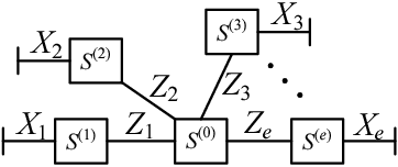
Before describing the decoding algorithm, we introduce the message processing/passing algorithm over a general normal graph [27]. The notation is closely related to that used in [28, 29]. As shown in Fig. 2, a general normal graph can be used to represent a system, where vertices represent subsystems and edges represent variables. All edges (variables) connecting to a vertex (subsystem) must satisfy the specific constraints of the subsystem. For example, the subsystem is connected to via , and the subsystem is potentially connected to other system via a half edge . Associated with each edge is a message that is defined in this paper as the probability mass function (pmf) of the corresponding variable. We focus on random variables defined over . We use the notation to denote the message from vertex to vertex . Suppose that all messages are available. Then, the vertex , as a message processor, delivers the outgoing message with respect to any given by computing the likelihood function
| (7) |
Because the computation of the likelihood function is irrelevant to the incoming message
, we claim that is exactly the so-called extrinsic message. For simplicity, if two subsystems share multiple variables of the same type, the corresponding edges can be merged into one edge. Such an edge represents a sequence of random variables, whose messages are then collectively written in a sequence. Notice that such a simplified representation is just for the convenience of describing the message passing. For message processing, any edge that represents multiple random variables must be treated as multiple separated edges.

Fig. 3 shows the normal graph of a BMST system with and . There are four types of nodes in the normal graph of the BMST system, and each edge represents a sequence of random variables.
- •
Node C: The node C represents the constraint that must be a codeword of that corresponds to . In practice, is usually assumed to be independent and uniformly distributed over . Assume that the messages associated with are available from the node =. The node C performs a soft-in-soft-out (SISO) decoding algorithm to compute the extrinsic messages. The extrinsic messages associated with are fed back to the node =, while the extrinsic messages associated with can be used to make decisions on the transmitted data.
- •
Node =: The node = represents the constraint that all connecting variables must take the same realizations. The message processing/passing algorithm of the node = is the same as that of the variable node in an LDPC code.
- •
Node : The node represents the -th interleaver, which interleaves or de-interleaves the input messages.
- •
Node +: The node + represents the constraint that all connecting variables must be added up to zero over . The message processing/passing algorithm at the node + is similar to that at the check node in an LDPC code. The only difference is that the messages associated with the half edge are computed from the channel observations.
The normal graph of a BMST system can be divided into layers, where each layer typically consists of a node of type C, a node of type =, nodes of type , and a node of type +, see Fig. 3 for reference.
III-B Decoding Algorithm
For simplicity, we assume that is modulated using binary phase-shift keying (BPSK) with 0 and 1 mapped to and , respectively and transmitted over an additive white Gaussian noise (AWGN) channel, resulting in a received vector . In more general settings, we assume that the a posteriori probabilities are computable22 2 The computation in this step is irrelevant to the code constraints but depends only on the modulation and the channel., where is the -th component of .
After all for are received, an iterative forward-backward decoding can be implemented to obtain the decoding result . The algorithm is scheduled as follows.
Algorithm 2
Iterative Forward-Backward Decoding of BMST
- •
Initialization: Considering only the channel constraint, compute the a posteriori probabilities from the received vector for . All messages over the intermediate edges are initialized as uniformly distributed variables. Notice that for and . Set a maximum iteration number .
- •
Iteration: For , , , ,
- 1.
Forward recursion: For , , , , the -th layer performs a message processing/passing algorithm scheduled as
In the above procedure, the message processor at each node takes as input all available messages from connecting edges and delivers as output extrinsic messages to connecting edges. Hence the messages from adjacent layers are utilized, and the messages to adjacent layers are updated by considering both the constraints in the -th layer and the received vector .
- 2.
Backward recursion: For , , , , the -th layer performs a message processing/passing algorithm scheduled as
- 3.
Hard decision: For , make hard decisions on resulting in . If certain conditions are satisfied, output for and exit the iteration. Stopping criteria are discussed in Section III-C.
- 1.
The above algorithm (Algorithm 2) suffers from a large decoding delay for large . Similar to the Viterbi algorithm in practical systems, we present the following iterative sliding-window decoding with a fixed decoding delay . In contrast to Algorithm 2, the iterative sliding-window algorithm with decoding delay works over a subgraph consisting of consecutive layers, which delivers, at time , as output the estimated data block after is received and slides into the decoder. Usually, we take the decoding delay . The schedule is described as follows.
Algorithm 3
Iterative Sliding-window Decoding of BMST
- •
Global initialization: Assume that have been received. Considering only the channel constraint, compute the a posteriori probabilities from the received vector for . All messages over the other edges within and connecting to the -th layer () are initialized as uniformly distributed variables. Set a maximum iteration number .
- •
Sliding-window decoding: For , , , ,
- 1.
Local initialization: If , compute the a posteriori probabilities from the received vector and all messages over other edges within and connecting to the -th layer are initialized as uniformly distributed variables.
- 2.
Iteration: For , , , ,
- (a)
Forward recursion: For , , , , the -th layer performs a message processing/passing algorithm scheduled as
- (b)
Backward recursion: For , , , , the -th layer performs a message processing/passing algorithm scheduled as
- (c)
Hard decision: Make hard decisions on resulting in . If certain conditions are satisfied, output and exit the iteration. Stopping criteria are discussed in Section III-C.
- (a)
- 3.
Cancelation: Remove the effect of on all layers by updating the a posteriori probabilities as
(8) for and .
- 1.
III-C Stopping Criteria
III-C1 Entropy-Based Stopping Criterion
As the error-detection ability of short codes is usually weak, the entropy-based stopping criterion [28] is used. The entropy-based stopping criterion is described as follows.
The entropy-based stopping criterion for Algorithm 2: Before the iteration, we set a threshold and initialize the entropy rate , where is the random vector corresponding to . For each iteration , estimate the entropy rate of by
| (9) |
where,
| (10) |
and are computed at the node +. If , exit the iteration.
The entropy-based stopping criterion for Algorithm 3: Before the iteration, we set a threshold and initialize the entropy rate , where is the random vector corresponding to . For each iteration , estimate the entropy rate of by
| (11) |
where, is computed by (10) and are computed at the node +. If , exit the iteration.
III-C2 Parity-Check-Based Stopping Criterion
To avoid the extra computational complexity caused by estimating the entropy rate, we may take a concatenated code as the basic code, where the outer code is a powerful error-detection code (say cyclic redundancy check (CRC) code) and the inner code is a short code. In this situation, the SISO algorithm for the basic code is performed by ignoring the constraint specified by the outer code. In the process of the iterative decoding, once the decoding output of the inner code is a valid codeword of the outer code, report a decoding success and exit the iteration.
III-D List Decoding after Iteration
The use of error-detection codes for early stopping incurs a rate loss, however, it can be used to obtain extra coding gain by list decoding [30, 31]. In the case when the decoding fails after iterations, the list decoding algorithm for the inner code takes as input and generates a list of outputs. Once one output in the list is found to be a valid codeword of the outer code, report a decoding success and exit the iteration.
IV Performance Analysis
The objective of this section is to analyze the “extra” coding gain over the basic code by the BMST system. Before doing this, we need to point out that the “extra” coding gain may be negative in the high bit-error-rate (BER) region due to the possible error propagation. Let be the performance function of the basic code , where is the BER and in dB. Since is short, we assume that is available. For example, if is a terminated convolutional code, the performance function under the maximum a posteriori probability (MAP) decoding can be evaluated by performing the Bahl-Cocke-Jelinek-Raviv (BCJR) algorithm [32]. Let be the performance function corresponding to the BMST system.
IV-A Genie-Aided Lower Bound on BER
Let be the transmitted data. To derive the lower bound, we assume the MAP decoder for the BMST system, which in principle computes (by Bayes’ rule)
| (12) |
for all and , where the summation is over all . We know that if , the decoding output is correct for this considered bit. In the meanwhile, we assume a genie-aided decoder, which computes for all and with the transmitted data available. Likewise, if , the decoding output is correct for this considered bit. For a specific and , it is possible that . However, the expectation
| (13) |
where is the conditional mutual information, implying that the genie-aided decoder performs statistically better than the MAP decoder of the BMST system. As a result, the BER performance can be lower-bounded by, taking into account the rate loss,
| (14) |
where the last equality holds from the fact that the data block is encoded and transmitted times from the perspective of the genie-aided decoder.
Furthermore, noticing that for the transmitted data block in the low error rate region, we have from (12) that and hence can expect that
| (15) |
as increases. That is, the maximum coding gain can be dB for large in the low error rate region.
IV-B Upper Bound on BER
To upper-bound the BER performance, we present a method to compute the IOWEF of the BMST system. Let the IOWEF of the basic code be given as
| (16) |
where , are two dummy variables and denotes the number of codewords having a Hamming weight when the corresponding input information sequence having a Hamming weight . Similarly, denote by the IOWEF of the BMST system. We have
| (17) | |||||
where represents the Hamming weight and the summation is over all possible data sequences with for . Since it is a sum of products, can be computed in principle by a trellis-based algorithm over the polynomial ring. For specific interleavers, the trellis has a state space of size . To make the computation tractable, we turn to an ensemble of BMST system by assuming that the interleavers are chosen independently and uniformly at random for each transmission block . With this assumption, we can see that is a random variable that depends on the Hamming weights .
In the following, we take as an example to describe the algorithm for computing the IOWEF of the defined ensemble of the BMST system. We can see that is a random variable which is sensitive to neither nor but depends only on their Hamming weights and . To be precise, we have
| (18) |
with probability
| (19) |
where
| (20) |
The trellis is time-invariant. At stage , the trellis has states, each of which records the Hamming weight . Emitting from each state there are branches, each of which corresponds to the Hamming weight . To each branch , we assign a “metric”
| (21) |
Then can be calculated recursively by performing a forward trellis-based algorithm [33] over the polynomial ring as follows.
Algorithm 4
Computing IOWEF of BMST with
- 1.
Initialize , .
- 2.
For , , , ,
where .
- 3.
At time , we have .
Given , the upper bound for the BER of the BMST system can be calculated by an improved union bound [34].
Remark. For , the computation becomes more complicated due to the huge number of trellis states . Fortunately, as shown in [34], truncated IOWEF suffices to give a valid upper bound, a fact that can be used to simplify the computation by removing certain states from the trellis.
V Numerical Results
In this section, we present BMST examples with different types of basic codes. All simulations are conducted by assuming BPSK modulation and AWGN channels. In all the examples, we set as the maximum number of iterations. In the examples where the entropy-based stopping criterion is used, we set as the threshold. Without specification, the iterative sliding-window algorithm (Algorithm 3) is used for decoding and S-random interleavers [35] (randomly generated but fixed) with parameter are used for encoding. Here stands for the maximum integer that is not greater than .
V-A Short Convolutional Codes as Basic Codes
In this subsection, the BCJR algorithm is performed as the SISO decoding algorithm for basic codes and the entropy-based stopping criterion is used.


Example 1
The basic code is a terminated systematic encoded 4-state convolutional code (CC) defined by the polynomial generator matrix with dimension and length . We take for encoding. The decoding is performed after all are received (Algorithm 2). Fig. 4 shows the spectrum of the ensemble of the BMST system, where
| (22) |
For comparison, the spectrum of the independent transmission system (with code book
instead of the BMST code book ) is also shown in Fig. 4. We can see that the spectrum of the BMST system has less number of codewords with small Hamming weights, indicating that the BMST system has potentially better performance than the independent transmission system. Simulation results are shown in Fig. 5, which match well with the bounds in the high signal-to-noise ratio (SNR) region. This also indicates that the iterative forward-backward algorithm is near optimal in the high SNR region.

Example 2
The basic code is a terminated 4-state convolutional code defined by the polynomial generator matrix with and . Simulations results for are shown in Fig. 6. We can see that 1) given the encoding memory , the performance can be improved by increasing the decoding delay and 2) the performance in the high SNR region can be improved by increasing .
V-B Short Block Codes as Basic Codes
In this subsection, the BCJR algorithm is performed as the SISO decoding algorithm for basic codes and the entropy-based stopping criterion is used.

Example 3
The basic code is the Cartesian product of Hamming code with and . Simulation results for and are shown in Fig. 7. We can see that the BMST system of the Hamming code has a similar behavior to the BMST system of the convolutional code in Example 2. With and , an extra coding gain of dB is obtained at BER .
Example 4
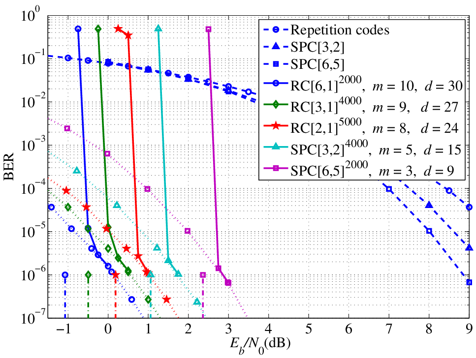
The basic code is either the Cartesian product of a repetition code (RC), denoted by , or the Cartesian product of a single parity-check (SPC) code, denoted by . Simulation results with for all BMST systems are shown in Fig. 8. Also shown in Fig. 8 are the Shannon limits. More precisely, the Shannon limit of a code rate is depicted as a vertical dashed line, which shares the same mark with the solid performance curve of the given code rate. We can see that, given a short code, the corresponding Shannon limit can be approached using the BMST system by choosing properly the encoding memory and the decoding delay. There is about 0.5 dB away from the respective Shannon limit at BER= for all BMST systems given in Fig. 8.
V-C Concatenation of CRC Codes and Short Convolutional Codes as Basic Codes
If a concatenated code with a powerful error-detection outer code is used as the basic code, we can use the parity-check-based stopping criterion for early stopping. In this case, the SISO algorithm for the basic code is performed by ignoring the outer code. To improve the performance, a list decoding can be implemented after the iteration.

Example 5
The basic code is a concatenated code with and , where the outer code is a 32-bit CRC code and the inner code is a terminated 4-state convolutional code defined by the polynomial generator matrix . Simulation results for are shown in Fig. 9. We can see that the simulation results are similar to those in Example 2. The BER curves match well with the lower bounds derived from the BCJR-only curves but diverge from the bounds derived from the list-Viterbi (with list size 2) curves. The reason is as follows. During the iterative sliding-window decoding of BMST systems, the CRC code serves only as an error-detection code to exit the iteration at the right time and is less useful to enhance the error performance. To verify this, a list decoding with list size is implemented after the failure of the iterative sliding-window decoding. As expected, the simulation results match well with the bounds derived from the list-Viterbi curves. For an example, see the curve in Fig. 9 with and .
VI On the Universality of the BMST
VI-A Sketch of the Performance Curve

We have conducted lots of simulations for BMST systems with a variety of basic codes while only some of them are presented in this paper due to the space limit. We have found that all simulations deliver performance curves that have similar behavior. That is, the performance curve drops down to the derived genie-aided lower bound as the decoding delay increases. Let be the basic code, which is either a terminated convolutional code with a short constraint length or a Cartesian product of a short block code. In either case, we assume that is large enough. Fig. 10 sketches the performance curves for a general BMST system. Compared with the uncoded system, as the SNR increases, the basic code has an asymptotic coding gain (ACG) upper-bounded by dB. The performance curve of the BMST system with encoding memory is lower-bounded by shifting to left that of the basic code by . Hence we have an extra ACG of dB. As the encoding memory increases, the curve of the performance lower bound shifts to left further. However, the waterfall part of the simulated curve may shift to right a little bit due to the error propagation. Because of the same reason, the BMST system performs worse than the basic code in the low SNR region.
VI-B Nonlinear Codes as Basic Codes
From both the encoding process and the decoding process of the BMST system, we can see that the linearity of the basic code plays no essential roles. What we need is an encoding algorithm as well as an SISO decoding algorithm for the basic code. Hence, from the theoretical point of view, we are interested in the performance of BMST system with a nonlinear basic code. The advantage of the use of the nonlinear code is that the same coding gain may be obtained over the uncoded system with a less encoding memory provided the nonlinear basic code is better than the comparable linear basic code [5]. The disadvantage is that the table look-up encoding algorithm and the brute-force SISO decoding algorithm may be required for a general nonlinear basic code.
In the following example, we show that BMST can also be applied to nonlinear codes. Following [5], a nonlinear binary code is defined as a set of binary vectors of length , any two of which have a Hamming distance at least and some two of which have a Hamming distance . The code rate is and the ACG is upper-bounded by dB. If necessary, the word-error rate (WER) is used to measure the performance. The input to the encoder is an index (carrying information) for some codeword in the nonlinear basic code. The table look-up encoding algorithm for the basic code is implemented in Algorithm 1. The brute-force MAP decoding algorithm based on Bayes’ rule is implemented as the SISO decoding algorithm for the nonlinear basic code in the iterative sliding-window decoding algorithm. The entropy-based stopping criterion is used.

Example 6
The basic code is the Cartesian product of the optimum Nordstrom-Robinson (NR) nonlinear code [36, 37]. As pointed out in [5], the Nordstrom-Robinson nonlinear code contains (at least) twice as many codewords as any linear code with the same length and minimum distance. Simulation results for are shown in Fig. 11. We can see that the performance curves of the BMST with this nonlinear code match well with the corresponding lower bounds in the high SNR region, which are consistent with sketches as shown in Fig. 10 for the general BMST system.
VI-C Concatenated Codes as Basic Codes
An inevitable but interesting question is whether the BMST is applicable to long codes. In this subsection, we present a BMST system with a concatenated code as the basic code, where the outer is a Reed-Solomon (RS) and the inner code is a convolutional code. The issue of this system is that no efficient SISO decoding algorithm for the basic code exists 33 3 Hence, we do not have the simple genie-aided lower bound in this case.. As a trade-off, we implement the iterative sliding-window decoding algorithm by ignoring the existence of the outer code, which is used only for removing the residual errors and stopping the iterations at the right time. For each iteration, the outer decoder (the Berlekamp-Massey (BM) [38, 39] algorithm) is performed. Whenever it is successful, the estimated data are output and the iteration is stopped.

Example 7
The basic code is the Consultative Committee on Space Data System (CCSDS) standard code [40] with and , where the outer code is a [255, 223] RS code over and the inner code is a terminated 64-state convolutional code defined by the polynomial generator matrix . The RS code not only removes the possible residual errors after the iterative sliding-window decoding of the inner code but also ensures (with high probability) the correctness of successfully decoded codewords.44 4 The mis-correction probability can be analyzed in a similar way to that given in [41]. The simulation results with , , and are shown in Fig. 12. We can see that, although we are unable to simulate the performance in the extremely low BER region, the extra coding gain is about dB at BER . Also notice that the BMST system performs worse than the basic code in the high BER region due to the error propagation.
VII Conclusion
In this paper, we presented more details about the block Markov superposition transmission (BMST), a construction of big convolutional codes from short codes. The encoding process can be as fast as the short code, while the decoding has a fixed delay. The coding gain of the BMST system is analyzed and verified by simulations. A nice property of the BMST is that its performance in the high SNR region can be approximately predicted. With several examples, we show that the BMST is a simple and general method for obtaining extra coding gain in the low BER region over short codes. With repetition codes and single parity-check codes as basic codes, the BMST system can approach the Shannon limit at BER within 0.5 dB for a wide range of code rates.
Acknowledgment
The authors are grateful to Prof. Baoming Bai from Xidian University for useful discussions.
References
- [1] P. Elias, “Coding for noisy channels,” IRE Conv. Rec., vol. 3, pp. 37–46, 1955.
- [2] D. J. Costello, Jr., J. Hagenauer, H. Imai, and S. B. Wicker, “Applications of error-control coding,” IEEE Trans. Inform. Theory, vol. 44, pp. 2531–2560, Oct. 1998.
- [3] A. J. Viterbi, “Error bounds for convolutional codes and an asymptotically optimum decoding algorithm,” IEEE Trans. Inform. Theory, vol. 13, pp. 260–269, Apr. 1967.
- [4] O. M. Collins, “The subtleties and intricacies of building a constraint length 15 convolutional decoder,” IEEE Trans. Commun., vol. 40, pp. 1810–1819, Dec. 1992.
- [5] F. J. MacWilliams and N. J. A. Sloane, The theory of error-correcting codes. Amsterdam, The Netherlands: North Holland, 1977.
- [6] P. Elias, “Error-free coding,” IRE Trans. Inform. Theory, vol. 4, pp. 29–37, Sept. 1954.
- [7] G. D. Forney, Jr., Concatenated codes. Cambridge, MA: MIT Press, 1966.
- [8] C. Berrou, A. Glavieux, and P. Thitimajshima, “Near Shannon limit error-correcting coding and decoding: Turbo codes,” in Proc. Int. Communications Conf. (ICC’93), Geneva, Switzerland, May 1993, pp. 1064–1070.
- [9] S. Benedetto and G. Montorsi, “Unveiling turbo codes: Some results on parallel concatenated coding schemes,” IEEE Trans. Inform. Theory, vol. 42, pp. 409–428, Mar. 1996.
- [10] S. Benedetto, D. Divsalar, G. Montorsi, and F. Pollara, “Serial concatenation of interleaved codes: Performance analysis, design, and iterative decoding,” IEEE Trans. Inform. Theory, vol. 44, pp. 909–926, May 1998.
- [11] D. Divsalar, H. Jin, and R. J. McEliece, “Coding theorems for ‘turbo-like’ codes,” in Proc. 36th Annu. Allerton Conf. Communications, Control, and Computing, Urbana, IL, Sept. 1998, pp. 201–210.
- [12] L. Ping, X. Huang, and N. Phamdo, “Zigzag codes and concatenated zigzag codes,” IEEE Trans. Inform. Theory, vol. 47, pp. 800–807, Feb. 2001.
- [13] A. Abbasfar, D. Divsalar, and K. Yao, “Accumulate-repeat-accumulate codes,” IEEE Trans. Commun., vol. 55, pp. 692–702, Apr. 2007.
- [14] S. Tong, L. Ping, and B. Bai, “Near Shannon limit precoded concatenated zigzag codes,” in Proc. Int. Symp. Turbo Codes and Iterative Information Processing, Gothenburg, Sweden, Aug. 2012, pp. 126–130.
- [15] R. G. Gallager, Low-Density Parity-Check Codes. Cambridge, MA: MIT Press, 1963.
- [16] D. J. C. MacKay, “Good error-correcting codes based on very sparse matrices,” IEEE Trans. Inform. Theory, vol. 45, pp. 399–431, Mar. 1999.
- [17] T. J. Richardson, M. A. Shokrollahi, and R. L. Urbanke, “Design of capacity-approaching irregular low-density parity-check codes,” IEEE Trans. Inform. Theory, vol. 47, pp. 619–637, Feb. 2001.
- [18] Y. Kou, S. Lin, and M. Fossorier, “Low-density parity-check codes based on finite geometries: A rediscovery and new results,” IEEE Trans. Inform. Theory, vol. 47, pp. 2711 –2736, Nov. 2001.
- [19] L. Lan, L. Zeng, Y. Tai, L. Chen, S. Lin, and K. Abdel-Ghaffar, “Construction of quasi-cyclic LDPC codes for AWGN and binary erasure channels: A finite field approach,” IEEE Trans. Inform. Theory, vol. 53, pp. 2429–2458, Jul. 2007.
- [20] A. J. Felström and K. S. Zigangirov, “Time-varying periodic convolutional codes with low-density parity-check matrix,” IEEE Trans. Inform. Theory, vol. 45, pp. 2181–2191, Sept. 1999.
- [21] A. E. Pusane, R. Smarandache, P. O. Vontobel, and D. J. Costello, “Deriving good LDPC convolutional codes from LDPC block codes,” IEEE Trans. Inform. Theory, vol. 57, pp. 835–857, Feb. 2011.
- [22] X. Ma, C. Liang, K. Huang, and Q. Zhuang, “Obtaining extra coding gain for short codes by block Markov superposition transmission,” in Proc. IEEE Int. Symp. Inf. Theory, Istanbul, Turkey, Jul. 2013, pp. 2054–2058.
- [23] T. M. Cover and C. S. K. Leung, “An achievable rate region for the multiple-access channel with feedback,” IEEE Trans. Inform. Theory, vol. 27, pp. 292–298, May 1981.
- [24] T. M. Cover and A. A. El Gamal, “Capacity theorems for the relay channel,” IEEE Trans. Inform. Theory, vol. 25, pp. 572–584, Sept. 1979.
- [25] F. M. J. Willems and E. C. van der Meulen, “The discrete memoryless multiple-access channel with cribbing encoders,” IEEE Trans. Inform. Theory, vol. 31, pp. 313–327, May 1985.
- [26] R. Johannesson and K. S. Zigangirov, Fundamentals of convolutional coding. Piscataway, NJ: IEEE Press, 1999.
- [27] G. D. Forney, Jr., “Codes on graphs: Normal realizations,” IEEE Trans. Inform. Theory, vol. 47, pp. 520–548, Feb. 2001.
- [28] X. Ma and L. Ping, “Coded modulation using superimposed binary codes,” IEEE Trans. Inform. Theory, vol. 50, pp. 3331–3343, Dec. 2004.
- [29] X. Ma, K. Zhang, H. Chen, and B. Bai, “Low Complexity X-EMS Algorithms for Nonbinary LDPC Codes,” IEEE Trans. Commun., vol. 60, pp. 9–13, Jan. 2012.
- [30] P. Elias, “List decoding for noisy channels,” in WESCON Conv. Rec., Res. Lab. Electron., MIT, Cambridge, MA, 1957, pp. 94–104.
- [31] J. M. Wozencraft, “List decoding,” in Quart. Progr. Rep., vol. 48, Res. Lab. Electron., MIT, Cambridge, MA, 1958.
- [32] L. R. Bahl, J. Cocke, F. Jelinek, and J. Raviv, “Optimal decoding of linear codes for minimizing symbol error rate,” IEEE Trans. Inform. Theory, vol. 20, pp. 284–287, Mar. 1974.
- [33] X. Ma and A. Kavčić, “Path partition and forward-only trellis algorithms,” IEEE Trans. Inform. Theory, vol. 49, pp. 38–52, Jan. 2003.
- [34] X. Ma, J. Liu, and B. Bai, “New techniques for upper-bounding the ML decoding performance of binary linear codes,” IEEE Trans. Commun., vol. 61, pp. 842–851, Mar. 2013.
- [35] S. Dolinar and D. Divsalar, “Weight distributions for turbo codes using random and nonrandom permutations,” TDA Progr. Rep. 42, vol. 122, pp. 56–65, Aug. 1995.
- [36] A. W. Nordstrom and J. P. Robinson, “An optimum nonlinear code,” Inform. Control., vol. 11, pp. 613–616, Nov.-Dec. 1967.
- [37] F. P. Preparata, “A class of optimum nonlinear double-error-correcting codes,” Inform. Control., vol. 13, pp. 378–400, Oct. 1968.
- [38] E. R. Berlekamp, Algebraic Coding Theory. New York: McGraw-Hill, 1968.
- [39] J. L. Massey, “Shift-register synthesis and BCH decoding,” IEEE Trans. Inform. Theory, vol. 15, pp. 122–127, Jan. 1969.
- [40] TM Synchronization and Channel Coding. The Consultative Committee for Space Data Systems (CCSDS) recommended standard, Aug. 2011.
- [41] X. Ma, K. Zhang, B. Bai, and X. Zhang, “Serial concatenation of RS codes with Kite codes: Performance analysis, iterative decoding and design.” [Online]. Available: http://arxiv.org/abs/1104.4927