跳到论文正文
W Papers独立论文阅读器 arXiv:1308.4794 论文正文 计算阅读时间 · 0%
引用这篇论文根据当前论文元数据生成,正式投稿前建议核对。


License: arXiv.org perpetual non-exclusive license
arXiv:1308.4794v2 [hep-ph] 29 Oct 2013

RESCEU-41/13

YITP-13-39

Langevin description of gauged scalar fields in a thermal bath

Yuhei Miyamoto1,2 Email: miyamoto”at”resceu.s.u-tokyo.ac.jp Affiliation: 1 Department of Physics, Graduate School of Science,
The University of Tokyo, Tokyo 113-0033, Japan
2 Research Center for the Early Universe (RESCEU),
Graduate School of Science, The University of Tokyo, Tokyo 113-0033, Japan
3 Yukawa Institute for Theoretical Physics,
Kyoto University, Kyoto 606-8502, Japan
4 Kavli Institute for the Physics and Mathematics of the Universe (WPI),
The University of Tokyo, Kashiwa, Chiba, 277-8568, Japan
   Hayato Motohashi2,3 Email: motohashi”at”resceu.s.u-tokyo.ac.jp Affiliation: 1 Department of Physics, Graduate School of Science,
The University of Tokyo, Tokyo 113-0033, Japan
2 Research Center for the Early Universe (RESCEU),
Graduate School of Science, The University of Tokyo, Tokyo 113-0033, Japan
3 Yukawa Institute for Theoretical Physics,
Kyoto University, Kyoto 606-8502, Japan
4 Kavli Institute for the Physics and Mathematics of the Universe (WPI),
The University of Tokyo, Kashiwa, Chiba, 277-8568, Japan
   Teruaki Suyama2 Email: suyama”at”resceu.s.u-tokyo.ac.jp Affiliation: 1 Department of Physics, Graduate School of Science,
The University of Tokyo, Tokyo 113-0033, Japan
2 Research Center for the Early Universe (RESCEU),
Graduate School of Science, The University of Tokyo, Tokyo 113-0033, Japan
3 Yukawa Institute for Theoretical Physics,
Kyoto University, Kyoto 606-8502, Japan
4 Kavli Institute for the Physics and Mathematics of the Universe (WPI),
The University of Tokyo, Kashiwa, Chiba, 277-8568, Japan
   Jun’ichi Yokoyama2,4 Email: yokoyama”at”resceu.s.u-tokyo.ac.jp Affiliation: 1 Department of Physics, Graduate School of Science,
The University of Tokyo, Tokyo 113-0033, Japan
2 Research Center for the Early Universe (RESCEU),
Graduate School of Science, The University of Tokyo, Tokyo 113-0033, Japan
3 Yukawa Institute for Theoretical Physics,
Kyoto University, Kyoto 606-8502, Japan
4 Kavli Institute for the Physics and Mathematics of the Universe (WPI),
The University of Tokyo, Kashiwa, Chiba, 277-8568, Japan
Abstract

We study the dynamics of the oscillating gauged scalar field in a thermal bath. A Langevin type equation of motion of the scalar field, which contains both dissipation and fluctuation terms, is derived by using the real-time finite temperature effective action approach. The existence of the quantum fluctuation-dissipation relation between the non-local dissipation term and the Gaussian stochastic noise terms is verified. We find the noise variables are anti-correlated at equal-time. The dissipation rate for the each mode is also studied, which turns out to depend on the wavenumber.

I Introduction

Recent advancements in observational technology enable us to trace back the history of the Universe. In particular, observations of the cosmic microwave background, including the latest results of the Planck mission [1], provide us with the picture of the Universe at the recombination, the subsequent evolution, and a piece of information on the early Universe. The Universe in a much earlier period, however, is still veiled and many models which are built to explain the physics beyond the energy scale realized in laboratories remain unverified. To select the theory describing our world, we need not only observational developments but also more precise theoretical predictions using fundamental theories of physics.

One of the most interesting phenomena in the early Universe is the phase transition. It has provided mechanisms of inflation [2, 3, 4, 5, 6, 7], called “old inflation” [3, 4] and “new inflation” [5, 6]. In both of the models inflation is driven by the vaccum energy before the end of the phase transition. The thermal inflation [8], also caused by the potential energy of the flaton field, is a relatively short accelerating period after the primordial inflation. Since it changes the expansion history of the Universe, not only the moduli and gravitinos are diluted but also the primordial gravitational waves are damped [9]. On the other hand, collisions of bubbles generated during a phase transition can produce gravitational waves [10]. Furthermore, depending on the kinds of the broken symmetry, various topological defects are expected to be produced. Among them, line-like topological defects known as cosmic strings can produce gravitational waves [11] which may be detectable by future experiments [12]. These examples indicate that the phase transition is a key to understand high-energy physics and the early Universe.

Precise description of the dynamics of phase transitions is necessary to compare predictions of each theoretical model with observations. In many models of the early Universe, phase transitions are controlled by the expectation value of the scalar fields. While the effective potential is a useful quantity to derive properties of the phase transitions that happen quasi-statically, its use often comes short because of dynamical nature of the scalar fields. In such cases, we need to directly solve the evolution equations of the scalar fields derived from the effective action. It has been shown that the behavior of a scalar field in thermal bath can be described by the Langevin equation [13], which includes stochastic noise terms coming from interactions with other fields in thermal bath. These noise terms may change the types of phase transitions. For example, a previous study [14] indicates that the fermionic noise may lead to the phase mixing, which cannot be described by the effective potential.

So far, the effective action and the resultant equation of motion of a scalar field has been studied in models where it has self-interaction and interactions with other fermions and scalar bosons [14, 15]. Now, it is an interesting project to extend the previous studies to include interactions with gauge fields. We extend previous analyses to include interactions with gauge fields using the simplest Abelian gauge theory known as scalar quantum electrodynamics. Though the hot scalar QED theory has been studied by Ref. [16, 17] to study the dynamics of gauge fields, we focus on the scalar field as a system of interest and treat gauge fields as a hot environment.

The organization of this paper is as follows. We briefly review the effective action method and apply it to the scalar quantum electrodynamics in Section II. Actually, this effective action contains the imaginary part. In Section III, we interpret it as stochastic noises and derive a generalized Langevin equation. We consider the meaning of the equation, and explain the validity of this interpretation. We also show the stochastic property of the noise, and compare it with the fermionic and scalar bosonic noises which have been studied in previous studies. The dissipation rate of the each mode is also studied. We summarize our study and discuss its applicability in Section IV.

II Effective action

As we have mentioned in the inrtoduction, one of our goals is the precise description of phase transitions in gauge theory which requires our knowledge of effective action for scalar field. In this paper, we focus on the derivation of the effective action and investigation of basic properties of the obtained equation of motion for the massive charged scalar field due to interactions with gauge fields. In order to realize phase transition, we need to add self-interaction of the scalar field to have Higgs mechanism. We defer the inclusion of the self-interaction to another study. The simplest approach to describe phase transitions in the hot early Universe is to analyze a finite-temperature effective potential. By using the effective potential, we can explain the symmetry restoration at high temperature or in the early Universe and the subsequent spontaneous symmetry breaking. However, since it is derived on the assumption of static, homogeneous field configuration, it cannot describe the dynamics of phase transitions accurately. In this section, in order to obtain the equation of motion governing the dynamical phenomenon, we calculate the effective action. Studies so far show that effective action generally contains the imaginary part, which can be interpreted as the origin of dissipative properties.

II.1 Settings

To clarify the role of gauge fields, we consider the scalar quantum electrodynamics, which is the simplest gauge theory. Its Lagrangian density is given by

ℒ=\displaystyle\mathcal{L}= Dμ​Φ†​Dμ​Φ−m2​Φ†​Φ−14​Fμ​ν​Fμ​ν\displaystyle D_{\mu}\Phi^{\dagger}D^{\mu}\Phi-m^{2}\Phi^{\dagger}\Phi-\frac{1}{4}F_{\mu\nu}F^{\mu\nu}
=\displaystyle= ∂μΦ†​∂μΦ−m2​Φ†​Φ−14​Fμ​ν​Fμ​ν\displaystyle\partial_{\mu}\Phi^{\dagger}\partial^{\mu}\Phi-m^{2}\Phi^{\dagger}\Phi-\frac{1}{4}F_{\mu\nu}F^{\mu\nu}
+i​e​Aμ​(Φ†​∂μΦ−Φ​∂μΦ†)+e2​Aμ​Aμ​Φ†​Φ.\displaystyle+ieA_{\mu}(\Phi^{\dagger}\partial^{\mu}\Phi-\Phi\partial^{\mu}\Phi^{\dagger})+e^{2}A_{\mu}A^{\mu}\Phi^{\dagger}\Phi\,. (1)

After imposing the Coulomb gauge condition ∇→⋅A→=0\vec{\nabla}\cdot\vec{A}=0, one can see the Lagrangian density becomes

ℒ=\displaystyle\mathcal{L}= ∂μΦ†​∂μΦ−m2​Φ†​Φ+12​∂μA→T⋅∂μA→T\displaystyle\partial_{\mu}\Phi^{\dagger}\partial^{\mu}\Phi-m^{2}\Phi^{\dagger}\Phi+\frac{1}{2}\partial_{\mu}\vec{A}_{T}\cdot\partial^{\mu}\vec{A}_{T}
−i​e​A→T​(Φ​∇→​Φ†−Φ†​∇→​Φ)−e2​A→T⋅A→T​Φ†​Φ\displaystyle-ie\vec{A}_{T}(\Phi\vec{\nabla}\Phi^{\dagger}-\Phi^{\dagger}\vec{\nabla}\Phi)-e^{2}\vec{A}_{T}\cdot\vec{A}_{T}\Phi^{\dagger}\Phi
+12​(∇→​A0)2−i​e​A0​(Φ​Φ˙†−Φ†​Φ˙)+e2​A02​Φ†​Φ.\displaystyle+\frac{1}{2}(\vec{\nabla}A_{0})^{2}-ieA_{0}(\Phi\dot{\Phi}^{\dagger}-\Phi^{\dagger}\dot{\Phi})+e^{2}A_{0}^{2}\Phi^{\dagger}\Phi\,. (2)

Here, A→T\vec{A}_{\rm T} means the transverse components, which satisfy ∇→⋅A→T=0\vec{\nabla}\cdot\vec{A}_{\rm T}=0.

In the so-called real-time thermal field theory, we can calculate thermal average using path integral.*1*1 *1 One of the introductory textbooks is [18]. We can choose the time path so that it consists of three paths: (i)(i) A path from ti(<0)t_{i}\,\,(<0) to −ti-t_{i} on real axis of tt (plus contour), (i​i)(ii) a path from −ti-t_{i} to tit_{i} on real axis of tt (minus contour), and (i​i​i)(iii) a path from tit_{i} to ti−i​βt_{i}-i\beta, where β=1/T\beta=1/T is the inverse of the temperature. We can neglect the contribution from the third contour when taking T→∞T\rightarrow\infty [19]. We denote field variables on the contour (ii) and (i​iii) by superscripts ++ and −-, respectively. Following Boyanovsky et al. [17], thermal propagators for scalar field Φ\Phi and gauge field A→T\vec{A}_{\rm T} are given as follows.

Propagators for scalar field:

⟨Φ(a)†(x→,t)Φ(b)(x′→,t′)⟩=−i∫d3​k(2​π)3Gka​b(t,t′)e−ik→⋅(x→−x′→)\langle\Phi^{(a)\dagger}(\vec{x},t)\Phi^{(b)}(\vec{x^{\prime}},t^{\prime})\rangle=-i\int\frac{d^{3}k}{(2\pi)^{3}}G^{ab}_{k}(t,t^{\prime})e^{-i\vec{k}\cdot(\vec{x}-\vec{x^{\prime}})} (3)
Gk+⁣+​(t,t′)\displaystyle G^{++}_{k}(t,t^{\prime}) =Gk>​(t,t′)​Θ​(t−t′)+Gk<​(t,t′)​Θ​(t′−t)\displaystyle=G^{>}_{k}(t,t^{\prime})\Theta(t-t^{\prime})+G^{<}_{k}(t,t^{\prime})\Theta(t^{\prime}-t) (4)
Gk−⁣−​(t,t′)\displaystyle G^{--}_{k}(t,t^{\prime}) =Gk>​(t,t′)​Θ​(t′−t)+Gk<​(t,t′)​Θ​(t−t′)\displaystyle=G^{>}_{k}(t,t^{\prime})\Theta(t^{\prime}-t)+G^{<}_{k}(t,t^{\prime})\Theta(t-t^{\prime}) (5)
Gk+⁣−​(t,t′)\displaystyle G^{+-}_{k}(t,t^{\prime}) =−Gk<​(t,t′)\displaystyle=-G^{<}_{k}(t,t^{\prime}) (6)
Gk−⁣+​(t,t′)\displaystyle G^{-+}_{k}(t,t^{\prime}) =−Gk>​(t,t′)\displaystyle=-G^{>}_{k}(t,t^{\prime}) (7)
Gk>​(t,t′)\displaystyle G^{>}_{k}(t,t^{\prime}) =i2​ωk​[(1+nk)​e−i​ωk​(t−t′)+nk​e+i​ωk​(t−t′)]\displaystyle=\frac{i}{2\omega_{k}}\Big[(1+n_{k})e^{-i\omega_{k}(t-t^{\prime})}+n_{k}e^{+i\omega_{k}(t-t^{\prime})}\Big] (8)
Gk<​(t,t′)\displaystyle G^{<}_{k}(t,t^{\prime}) =i2​ωk​[nk​e−i​ωk​(t−t′)+(1+nk)​e+i​ωk​(t−t′)]\displaystyle=\frac{i}{2\omega_{k}}\Big[n_{k}e^{-i\omega_{k}(t-t^{\prime})}+(1+n_{k})e^{+i\omega_{k}(t-t^{\prime})}\Big] (9)
ωk=|k→|2+m2,nk=1eβ​ωk−1\omega_{k}=\sqrt{|\vec{k}|^{2}+m^{2}},\,n_{k}=\frac{1}{e^{\beta\omega_{k}}-1} (10)

Propagators for gauge field:

⟨AT​i(a)(x→,t)AT​j(b)(x′→,t′)⟩=−i∫d3​k(2​π)3𝒢k​i​ja​b(t,t′)e−ik→⋅(x→−x′→)\langle A_{Ti}^{(a)}(\vec{x},t)A_{Tj}^{(b)}(\vec{x^{\prime}},t^{\prime})\rangle=-i\int\frac{d^{3}k}{(2\pi)^{3}}{\mathcal{G}}^{ab}_{k\,ij}(t,t^{\prime})e^{-i\vec{k}\cdot(\vec{x}-\vec{x^{\prime}})} (11)
𝒢k​i​j+⁣+​(t,t′)\displaystyle{\mathcal{G}}^{++}_{k\,\,ij}(t,t^{\prime}) =𝒫i​j​(k→)​[gk>​(t,t′)​Θ​(t−t′)+gk<​(t,t′)​Θ​(t′−t)]\displaystyle={\mathcal{P}}_{ij}(\vec{k})\Big[g^{>}_{k}(t,t^{\prime})\Theta(t-t^{\prime})+g^{<}_{k}(t,t^{\prime})\Theta(t^{\prime}-t)\Big] (12)
𝒢k​i​j−⁣−​(t,t′)\displaystyle{\mathcal{G}}^{--}_{k\,\,ij}(t,t^{\prime}) =𝒫i​j​(k→)​[gk>​(t,t′)​Θ​(t′−t)+gk<​(t,t′)​Θ​(t−t′)]\displaystyle={\mathcal{P}}_{ij}(\vec{k})\Big[g^{>}_{k}(t,t^{\prime})\Theta(t^{\prime}-t)+g^{<}_{k}(t,t^{\prime})\Theta(t-t^{\prime})\Big] (13)
𝒢k​i​j+⁣−​(t,t′)\displaystyle{\mathcal{G}}^{+-}_{k\,\,ij}(t,t^{\prime}) =−𝒫i​j​(k→)​gk<​(t,t′)\displaystyle=-{\mathcal{P}}_{ij}(\vec{k})g^{<}_{k}(t,t^{\prime}) (14)
𝒢k​i​j−⁣+​(t,t′)\displaystyle{\mathcal{G}}^{-+}_{k\,\,ij}(t,t^{\prime}) =−𝒫i​j​(k→)​gk>​(t,t′)\displaystyle=-{\mathcal{P}}_{ij}(\vec{k})g^{>}_{k}(t,t^{\prime}) (15)
gk>​(t,t′)\displaystyle g^{>}_{k}(t,t^{\prime}) =i2​k​[(1+Nk)​e−i​k​(t−t′)+Nk​e+i​k​(t−t′)]\displaystyle=\frac{i}{2k}\Big[(1+N_{k})e^{-ik(t-t^{\prime})}+N_{k}e^{+ik(t-t^{\prime})}\Big] (16)
gk<​(t,t′)\displaystyle g^{<}_{k}(t,t^{\prime}) =i2​k​[Nk​e−i​k​(t−t′)+(1+Nk)​e+i​k​(t−t′)]\displaystyle=\frac{i}{2k}\Big[N_{k}e^{-ik(t-t^{\prime})}+(1+N_{k})e^{+ik(t-t^{\prime})}\Big] (17)
k=|k→|2,Nk=1eβ​k−1,𝒫i​j​(k→)=δi​j−ki​kjk2k=\sqrt{|\vec{k}|^{2}},\quad N_{k}=\frac{1}{e^{\beta k}-1},\quad{\mathcal{P}}_{ij}(\vec{k})=\delta_{ij}-\frac{k_{i}k_{j}}{k^{2}} (18)

The generating functional of Green’s function is

∫𝒟​A→T​𝒟​Φ​𝒟​Φ†​exp⁡[i​∫d4​x​{ℒ⁡[A→T(+),Φ(+),Φ†(+)]−ℒ⁡[A→T(−),Φ(−),Φ†(−)]}].\int\mathcal{D}\vec{A}_{T}\mathcal{D}\Phi\mathcal{D}\Phi^{\dagger}\exp\left[i\int d^{4}x\,\left\{\mathcal{L}[\vec{A}^{(+)}_{T},\,\Phi^{(+)},\,\Phi^{\dagger(+)}]-\mathcal{L}[\vec{A}^{(-)}_{T},\,\Phi^{(-)},\,\Phi^{\dagger(-)}]\right\}\right]\,. (19)

II.2 Perturbative expansion

Calculating the effective action corresponds to the summation of one-particle-irreducible diagrams. Practically, effective action can be obtained only by means of perturbative expansion in terms of the gauge coupling constant ee, which we adopt in our study. The lowest non-trivial contributions to the effective action appear at the second order of coupling constant ee. At this order, there are two relevant diagrams, which are shown in FIG. 1.

Refer to caption
Figure 1: 𝒪⁡(e2)\mathcal{O}(e^{2}) 1PI diagrams. The solid/wavy line represents the scalar/photon propagator, respectively. The left diagram produces non-local terms in the effective action. The right diagram gives a thermal correction to the mass term, which is proportional to T2T^{2}.

In addition to these 1PI diagrams, we have to rewrite A0A_{0} using its Euler-Lagrange equation as

A0​(x)\displaystyle A_{0}(x) =−1Δ​ρ​(x)+𝒪⁡(e2)\displaystyle=-\frac{1}{\Delta}\rho(x)+{\cal O}(e^{2}) (20)
ρ\displaystyle\rho ≡i​e​(Φ​Φ˙†−Φ†​Φ˙)\displaystyle\equiv ie(\Phi\dot{\Phi}^{\dagger}-\Phi^{\dagger}\dot{\Phi}) (21)

and take the interaction ℒint=12​ρ​1Δ​ρ{\cal L}_{\rm int}=\frac{1}{2}\rho\frac{1}{\Delta}\rho into account.

The contribution of the left diagram in FIG. 1 to the effective action Γ\Gamma is

Γ⊃\displaystyle\Gamma\supset +4ie2∫d4x1d4x2⟨AT​i(+)(x1)AT​j(+)(x2)⟩⟨∂iΦ†(+)(x1)∂jΦ(+)(x2)⟩Φ†(+)(x2)Φ(+)(x1)\displaystyle+4ie^{2}\int d^{4}x_{1}d^{4}x_{2}\,\Big<A^{(+)}_{Ti}(x_{1})A^{(+)}_{Tj}(x_{2})\Big>\Big<\partial_{i}\Phi^{\dagger(+)}(x_{1})\partial_{j}\Phi^{(+)}(x_{2})\Big>\Phi^{\dagger(+)}(x_{2})\Phi^{(+)}(x_{1})
+4ie2∫d4x1d4x2⟨AT​i(−)(x1)AT​j(−)(x2)⟩⟨∂iΦ†(−)(x1)∂jΦ(−)(x2)⟩Φ†(−)(x2)Φ(−)(x1)\displaystyle+4ie^{2}\int d^{4}x_{1}d^{4}x_{2}\,\Big<A^{(-)}_{Ti}(x_{1})A^{(-)}_{Tj}(x_{2})\Big>\Big<\partial_{i}\Phi^{\dagger(-)}(x_{1})\partial_{j}\Phi^{(-)}(x_{2})\Big>\Phi^{\dagger(-)}(x_{2})\Phi^{(-)}(x_{1})
−4ie2∫d4x1d4x2⟨AT​i(−)(x1)AT​j(+)(x2)⟩⟨∂iΦ†(−)(x1)∂jΦ(+)(x2)⟩Φ†(+)(x2)Φ(−)(x1)\displaystyle-4ie^{2}\int d^{4}x_{1}d^{4}x_{2}\,\Big<A^{(-)}_{Ti}(x_{1})A^{(+)}_{Tj}(x_{2})\Big>\Big<\partial_{i}\Phi^{\dagger(-)}(x_{1})\partial_{j}\Phi^{(+)}(x_{2})\Big>\Phi^{\dagger(+)}(x_{2})\Phi^{(-)}(x_{1})
−4ie2∫d4x1d4x2⟨AT​i(+)(x1)AT​j(−)(x2)⟩⟨∂iΦ†(+)(x1)∂jΦ(−)(x2)⟩Φ†(−)(x2)Φ(+)(x1),\displaystyle-4ie^{2}\int d^{4}x_{1}d^{4}x_{2}\,\Big<A^{(+)}_{Ti}(x_{1})A^{(-)}_{Tj}(x_{2})\Big>\Big<\partial_{i}\Phi^{\dagger(+)}(x_{1})\partial_{j}\Phi^{(-)}(x_{2})\Big>\Phi^{\dagger(-)}(x_{2})\Phi^{(+)}(x_{1})\,, (22)

and the right diagram contributes

Γ⊃−e2∫d4x[⟨AT​i(+)(x)AT​i(+)(x)⟩Φ†(+)(x)Φ(+)(x)−⟨AT​i(−)(x)AT​i(−)(x)⟩Φ†(+)(x)Φ(−)(x)].\Gamma\supset-e^{2}\int d^{4}x\Big[\Big<A^{(+)}_{Ti}(x)A^{(+)}_{Ti}(x)\Big>\Phi^{\dagger(+)}(x)\Phi^{(+)}(x)-\Big<A^{(-)}_{Ti}(x)A^{(-)}_{Ti}(x)\Big>\Phi^{\dagger(+)}(x)\Phi^{(-)}(x)\Big]\,. (23)

This local term gives a thermal correction to the mass term. *2*2 *2 Here we omit the divergent part, which is to be cancelled by a mass counter term since it exists even at zero temperature.

⟨AT​i(+)​(x)​AT​i(+)​(x)⟩=⟨AT​i(−)​(x)​AT​i(−)​(x)⟩=T26\Big<A^{(+)}_{Ti}(x)A^{(+)}_{Ti}(x)\Big>=\Big<A^{(-)}_{Ti}(x)A^{(-)}_{Ti}(x)\Big>=\frac{T^{2}}{6} (24)

From the interaction originally expressed by A0A_{0}, we obtain

Γ⊃\displaystyle\Gamma\supset −e2∫d4​k(2​π)4d4​p(2​π)4d4​q(2​π)41|p→|2(2k0−p0)(2q0−p0)\displaystyle-e^{2}\int\frac{d^{4}k}{(2\pi)^{4}}\frac{d^{4}p}{(2\pi)^{4}}\frac{d^{4}q}{(2\pi)^{4}}\frac{1}{|\vec{p}|^{2}}(2k_{0}-p_{0})(2q_{0}-p_{0})
×[⟨Φ~†(+)(k−p)Φ~(+)(q)⟩Φ~(+)(k)Φ~†(+)(q+p)\displaystyle\times\Big[\Big<\tilde{\Phi}^{\dagger(+)}(k-p)\tilde{\Phi}^{(+)}(q)\Big>\tilde{\Phi}^{(+)}(k)\tilde{\Phi}^{\dagger(+)}(q+p)
−⟨Φ~†(−)(k−p)Φ~(−)(q)⟩Φ~(−)(k)Φ~†(−)(q+p)].\displaystyle\quad-\Big<\tilde{\Phi}^{\dagger(-)}(k-p)\tilde{\Phi}^{(-)}(q)\Big>\tilde{\Phi}^{(-)}(k)\tilde{\Phi}^{\dagger(-)}(q+p)\Big]\,. (25)

It is convenient to replace Φ(±)\Phi^{(\pm)} with new variables

Φ(±)=ϕc±12​ϕΔ.\Phi^{(\pm)}=\phi_{c}\pm\frac{1}{2}\phi_{\Delta}\,. (26)

Finally the effective action Γ\Gamma incorporating these two diagrams and A0A_{0} terms up to the second order in ee becomes

Γ=\displaystyle\Gamma= ∫d4x[ϕΔ†(x)(−∂μ∂μ−m2−e2T26)ϕc(x)\displaystyle\int d^{4}x\,\Big[\phi_{\Delta}^{\dagger}(x)\left(-\partial_{\mu}\partial^{\mu}-m^{2}-e^{2}\frac{T^{2}}{6}\right)\phi_{c}(x)
+ϕΔ(x)(−∂μ∂μ−m2−e2T26)ϕc(x)†]\displaystyle\qquad\quad+\phi_{\Delta}(x)\left(-\partial_{\mu}\partial^{\mu}-m^{2}-e^{2}\frac{T^{2}}{6}\right)\phi_{c}(x)^{\dagger}\Big]
−4ie2∫d4x1d4x2∫d3​p1(2​π)3d3​p2(2​π)3e−i(p1→+p2→)⋅(x1→−x2→)𝒫i​j(p1→)p2​ip2​jΘ(t2−t1)\displaystyle-4ie^{2}\int d^{4}x_{1}d^{4}x_{2}\int\frac{d^{3}p_{1}}{(2\pi)^{3}}\frac{d^{3}p_{2}}{(2\pi)^{3}}e^{-i(\vec{p_{1}}+\vec{p_{2}})\cdot(\vec{x_{1}}-\vec{x_{2}})}\mathcal{P}_{ij}(\vec{p_{1}})p_{2i}p_{2j}\Theta(t_{2}-t_{1})
[gp1<​(t1,t2)​Gp2<​(t1,t2)−gp1>​(t1,t2)​Gp2>​(t1,t2)]​(ϕc†​(x1)​ϕΔ​(x2)+ϕc​(x1)​ϕΔ†​(x2))\displaystyle\qquad\big[g^{<}_{p_{1}}(t_{1},t_{2})G^{<}_{p_{2}}(t_{1},t_{2})-g^{>}_{p_{1}}(t_{1},t_{2})G^{>}_{p_{2}}(t_{1},t_{2})\big]\left(\phi_{c}^{\dagger}(x_{1})\phi_{\Delta}(x_{2})+\phi_{c}(x_{1})\phi_{\Delta}^{\dagger}(x_{2})\right)
−2ie2∫d4x1d4x2∫d3​p1(2​π)3d3​p2(2​π)3e−i(p1→+p2→)⋅(x1→−x2→)𝒫i​j(p1→)p2​ip2​j\displaystyle-2ie^{2}\int d^{4}x_{1}d^{4}x_{2}\int\frac{d^{3}p_{1}}{(2\pi)^{3}}\frac{d^{3}p_{2}}{(2\pi)^{3}}e^{-i(\vec{p_{1}}+\vec{p_{2}})\cdot(\vec{x_{1}}-\vec{x_{2}})}\mathcal{P}_{ij}(\vec{p_{1}})p_{2i}p_{2j}
[gp1<​(t1,t2)​Gp2<​(t1,t2)+gp1>​(t1,t2)​Gp2>​(t1,t2)]​ϕΔ†​(x1)​ϕΔ​(x2)\displaystyle\qquad\big[g^{<}_{p_{1}}(t_{1},t_{2})G^{<}_{p_{2}}(t_{1},t_{2})+g^{>}_{p_{1}}(t_{1},t_{2})G^{>}_{p_{2}}(t_{1},t_{2})\big]\phi_{\Delta}^{\dagger}(x_{1})\phi_{\Delta}(x_{2})
+ΓA0,\displaystyle+\Gamma_{A_{0}}\,, (27)
ΓA0=\displaystyle\Gamma_{A_{0}}= i​e2​∫d4​k(2​π)4​d4​q(2​π)4​(k0+q0)2|k→−q→|2​∫d​τ​ei​q0​τ​(Gq>​(τ)+Gq<​(τ))\displaystyle ie^{2}\int\frac{d^{4}k}{(2\pi)^{4}}\frac{d^{4}q}{(2\pi)^{4}}\frac{(k_{0}+q_{0})^{2}}{|\vec{k}-\vec{q}|^{2}}\int d\tau e^{iq_{0}\tau}(G^{>}_{q}(\tau)+G^{<}_{q}(\tau))
×12​(ϕc~​(k)​ϕΔ~†​(k)+ϕΔ~​(k)​ϕc~†​(k))\displaystyle\qquad\times\frac{1}{2}\left(\tilde{\phi_{c}}(k)\tilde{\phi_{\Delta}}^{\dagger}(k)+\tilde{\phi_{\Delta}}(k)\tilde{\phi_{c}}^{\dagger}(k)\right)
≡\displaystyle\equiv ∫d4​k(2​π)4​(ϕc~​(k)​ϕΔ~†​(k)+ϕΔ~​(k)​ϕc~†​(k))​f~A0​(k)\displaystyle\int\frac{d^{4}k}{(2\pi)^{4}}\left(\tilde{\phi_{c}}(k)\tilde{\phi_{\Delta}}^{\dagger}(k)+\tilde{\phi_{\Delta}}(k)\tilde{\phi_{c}}^{\dagger}(k)\right)\tilde{f}_{A_{0}}(k) (28)

Let us show that the imaginary part of the non-local terms which come from diagrams in FIG. 1 is nonzero. First, both of the integrands are invariant under replacements p1→→−p1→\vec{p_{1}}\rightarrow-\vec{p_{1}} and p2→→−p2→\vec{p_{2}}\rightarrow-\vec{p_{2}} respectively. This property allows us to replace e−i(p1→+p2→)⋅(x1→−x2→)e^{-i(\vec{p_{1}}+\vec{p_{2}})\cdot(\vec{x_{1}}-\vec{x_{2}})} with cos⁡[(p1→+p2→)⋅(x1→−x2→)]\cos\left[(\vec{p_{1}}+\vec{p_{2}})\cdot(\vec{x_{1}}-\vec{x_{2}})\right], which is real. Second, from Eqs. (8), (9), (16), and (17), we note that g<​G<−g>​G>g^{<}G^{<}-g^{>}G^{>} is purely imaginary and g<​G<+g>​G>g^{<}G^{<}+g^{>}G^{>} is real. Thus, the first non-local term is real and the second one is purely imaginary. In a similar way, we can see that ΓA0\Gamma_{A_{0}} is a real functional. We will explain how to interpret the imaginary part of the effective action in the next section.

III Langevin equation and Noise properties

In the previous section, we have seen the effective action for the scalar field contains an imaginary part as with the case of pure scalar theory in thermal environment. It can be written as

iΓ⊃−∫d4x1d4x2𝒩(x1−x2)(ϕΔ​R(x1)ϕΔ​R(x2)+ϕΔ​I(x1)ϕΔ​I(x2)),i\Gamma\supset-\int d^{4}x_{1}d^{4}x_{2}\,{\cal N}(x_{1}-x_{2})\left(\phi_{\Delta\,{\rm R}}(x_{1})\phi_{\Delta\,{\rm R}}(x_{2})+\phi_{\Delta\,{\rm I}}(x_{1})\phi_{\Delta\,{\rm I}}(x_{2})\right)\,, (29)

where

𝒩⁡(x1−x2)=\displaystyle{\cal N}(x_{1}-x_{2})= −2e2∫d3​p1(2​π)3d3​p2(2​π)3e−i(p1→+p2→)⋅(x1→−x2→)𝒫i​j(p1→)p2​ip2​j\displaystyle-2e^{2}\int\frac{d^{3}p_{1}}{(2\pi)^{3}}\frac{d^{3}p_{2}}{(2\pi)^{3}}e^{-i(\vec{p_{1}}+\vec{p_{2}})\cdot(\vec{x_{1}}-\vec{x_{2}})}\mathcal{P}_{ij}(\vec{p_{1}})p_{2i}p_{2j}
[gp1<​(t1,t2)​Gp2<​(t1,t2)+gp1>​(t1,t2)​Gp2>​(t1,t2)].\displaystyle\qquad\big[g^{<}_{p_{1}}(t_{1},t_{2})G^{<}_{p_{2}}(t_{1},t_{2})+g^{>}_{p_{1}}(t_{1},t_{2})G^{>}_{p_{2}}(t_{1},t_{2})\big]\,. (30)

ϕΔ​R/I\phi_{\Delta\,{\rm R/I}} are the real/imaginary part of ϕΔ\phi_{\Delta}, respectively. Now we are going to rewrite and interpret it as stochastic noise terms.

III.1 Mathematical transformation

As in previous studies[13, 14, 15], we rewrite the imaginary part by using Gaussian integral formula

exp[−∫d4xd4yφ(x)M(x,y)φ(y)]\displaystyle\exp\left[-\int d^{4}xd^{4}y\,\varphi(x)M(x,y)\varphi(y)\right]
∝\displaystyle\propto ∫𝒟ξexp[−14∫d4xd4yξ(x)M−1(x,y)ξ(y)+i∫d4xξ(x)φ(x)],\displaystyle\int\mathcal{D}\xi\exp\left[-\frac{1}{4}\int d^{4}xd^{4}y\,\xi(x)M^{-1}(x,y)\xi(y)+i\int d^{4}x\,\xi(x)\varphi(x)\right]\,, (31)

and interpret the integration over ξ\xi as an ensemble average, where ξ\xi is regarded as a stochastic Gaussian variable.

This formula is not applicable to arbitrary M⁡(x,y)M(x,y). Just like one dimensional Gaussian integral ∫d​x​exp⁡[−a​x2]\int dx\,\exp[-ax^{2}] requires a>0a>0, all of the eigenvalues of MM should be positive. After rewriting with Fourier transformations

∫d4​x​d4​y​ξ​(x)​M−1​(x,y)​ξ​(y)=∫d4​k(2​π)4​M~−1​(k)​|ξ~​(k)|2,\int d^{4}xd^{4}y\,\xi(x)M^{-1}(x,y)\xi(y)=\int\frac{d^{4}k}{(2\pi)^{4}}\tilde{M}^{-1}(k)|\tilde{\xi}(k)|^{2}\,, (32)

we notice that M~​(k)\tilde{M}(k) should be positive. The Fourier transformation of 𝒩\cal N with respect to t−t′t-t^{\prime} and x→−x→′\vec{x}-\vec{x}^{\prime} is

𝒩~​(ω,k→)=\displaystyle\tilde{\cal N}(\omega,\vec{k})= 2​e2​∫d3​p1(2​π)3​d3​p2(2​π)3​𝒫i​j​(p1→)​p2​i​p2​j​(2​π)3​δ​(k→−p1→−p2→)\displaystyle 2e^{2}\int\frac{d^{3}p_{1}}{(2\pi)^{3}}\frac{d^{3}p_{2}}{(2\pi)^{3}}\mathcal{P}_{ij}(\vec{p_{1}})p_{2i}p_{2j}(2\pi)^{3}\delta(\vec{k}-\vec{p_{1}}-\vec{p_{2}})
2​π2​p1​2​ωp2[{(1+Np1)(1+np2)+Np1np2}δ(ω−p1−ωp2)\displaystyle\quad\frac{2\pi}{2p_{1}2\omega_{p_{2}}}\Big[\bigl\{(1+N_{p_{1}})(1+n_{p_{2}})+N_{p_{1}}n_{p_{2}}\bigr\}\delta(\omega-p_{1}-\omega_{p_{2}})
+{(1+Np1)​np2+Np1​(1+np2)}​δ​(ω−p1+ωp2)\displaystyle\qquad\quad\quad+\bigl\{(1+N_{p_{1}})n_{p_{2}}+N_{p_{1}}(1+n_{p_{2}})\bigr\}\delta(\omega-p_{1}+\omega_{p_{2}})
+{Np1​(1+np2)+(1+Np1)​np2}​δ​(ω+p1−ωp2)\displaystyle\qquad\quad\quad+\bigl\{N_{p_{1}}(1+n_{p_{2}})+(1+N_{p_{1}})n_{p_{2}}\bigr\}\delta(\omega+p_{1}-\omega_{p_{2}})
+{Np1np2+(1+Np1)(1+np2)}δ(ω+p1+ωp2)].\displaystyle\qquad\quad\quad+\bigl\{N_{p_{1}}n_{p_{2}}+(1+N_{p_{1}})(1+n_{p_{2}})\bigr\}\delta(\omega+p_{1}+\omega_{p_{2}})\Big]\,. (33)

Clearly, this is positive for any (ω,k→)(\omega,\vec{k}), and thus this expression ensures us that we can use the formula (31) and rewrite the effective action with stochastic noise terms. Finally we obtain

ei​Γ=\displaystyle e^{i\Gamma}= ∫𝒟​ξa​𝒟​ξb​P​[ξa]​P​[ξb]​exp⁡[i​Γreal+i​∫d4​x​(ξa​(x)​ϕΔ​R​(x)+ξb​(x)​ϕΔ​I​(x))]\displaystyle\int{\mathcal{D}}\xi_{a}{\mathcal{D}}\xi_{b}\,P[\xi_{a}]P[\xi_{b}]\,\exp\Big[i\Gamma_{\rm real}+i\int d^{4}x(\xi_{a}(x)\phi_{\Delta\,{\rm R}}(x)+\xi_{b}(x)\phi_{\Delta\,{\rm I}}(x))\Big]
=\displaystyle= ∫𝒟​ξa​𝒟​ξb​P​[ξa]​P​[ξb]​exp⁡[i​Γreal+i​∫d4​x​(ξ†​(x)​ϕΔ​(x)+ξ⁡(x)​ϕΔ†​(x))]\displaystyle\int{\mathcal{D}}\xi_{a}{\mathcal{D}}\xi_{b}\,P[\xi_{a}]P[\xi_{b}]\,\exp\Big[i\Gamma_{\rm real}+i\int d^{4}x(\xi^{\dagger}(x)\phi_{\Delta}(x)+\xi(x)\phi_{\Delta}^{\dagger}(x))\Big]
≡\displaystyle\equiv ∫𝒟​ξa​𝒟​ξb​P​[ξa]​P​[ξb]​exp⁡[i​Seff],\displaystyle\int{\mathcal{D}}\xi_{a}{\mathcal{D}}\xi_{b}\,P[\xi_{a}]P[\xi_{b}]\,\exp\Big[iS_{\rm eff}\Big]\,, (34)

where

P⁡[ξa]=\displaystyle P[\xi_{a}]= exp[−14∫d4xd4yξa(x)𝒩−1(x−y)ξa(y)]\displaystyle\exp\Big[-\frac{1}{4}\int d^{4}xd^{4}y\,\xi_{a}(x){\cal N}^{-1}(x-y)\xi_{a}(y)\Big]
P⁡[ξb]=\displaystyle P[\xi_{b}]= exp[−14∫d4xd4yξb(x)𝒩−1(x−y)ξb(y)]\displaystyle\exp\Big[-\frac{1}{4}\int d^{4}xd^{4}y\,\xi_{b}(x){\cal N}^{-1}(x-y)\xi_{b}(y)\Big]
ξ=\displaystyle\xi= 12​ξa+i​12​ξb=ξR+i​ξI.\displaystyle\frac{1}{2}\xi_{a}+i\frac{1}{2}\xi_{b}=\xi_{\rm R}+i\xi_{\rm I}\,. (35)

Now we have a real action SeffS_{\rm eff} containing stochastic noise terms. The two-point correlation function of ξ\xi is given by

⟨ξR​(x1)​ξR​(x2)⟩=⟨ξI​(x1)​ξI​(x2)⟩=12​𝒩​(x1−x2)\langle\xi_{\rm R}(x_{1})\xi_{\rm R}(x_{2})\rangle=\langle\xi_{\rm I}(x_{1})\xi_{\rm I}(x_{2})\rangle=\frac{1}{2}{\mathcal{N}}(x_{1}-x_{2}) (36)
⟨ξR​(x1)​ξI​(x2)⟩=0\langle\xi_{\rm R}(x_{1})\xi_{\rm I}(x_{2})\rangle=0 (37)
⟨ξ⁡(x1)​ξ†​(x2)⟩=𝒩⁡(x1−x2).\langle\xi(x_{1})\xi^{\dagger}(x_{2})\rangle={\mathcal{N}}(x_{1}-x_{2})\,. (38)

III.2 Validity of interpretation and the fluctuation-dissipation relation

As we saw in the previous section, we obtain a real effective action SeffS_{\rm eff} by introducing noise terms. This real action leads to the following Langevin type equation of motion

(□+m2+e2​T26)​ϕc​(x)−∫d4​x′​fA0​(x−x′)​ϕc​(x′)\displaystyle\left(\Box+m^{2}+e^{2}\frac{T^{2}}{6}\right)\phi_{c}(x)-\int d^{4}x^{\prime}\,f_{A_{0}}(x-x^{\prime})\phi_{c}(x^{\prime})
+4ie2∫−∞tdt′∫d3x′∫d3​p1(2​π)3d3​p2(2​π)3e−i(p1→+p2→)⋅(x′→−x→)𝒫i​j(p1→)p2​ip2​j\displaystyle+4ie^{2}\int_{-\infty}^{t}dt^{\prime}\int d^{3}x^{\prime}\int\frac{d^{3}p_{1}}{(2\pi)^{3}}\frac{d^{3}p_{2}}{(2\pi)^{3}}e^{-i(\vec{p_{1}}+\vec{p_{2}})\cdot(\vec{x^{\prime}}-\vec{x})}\mathcal{P}_{ij}(\vec{p_{1}})p_{2i}p_{2j}
[gp1<​(t′,t)​Gp2<​(t′,t)−gp1>​(t′,t)​Gp2>​(t′,t)]​ϕc​(t′,x′→)\displaystyle\qquad\big[g^{<}_{p_{1}}(t^{\prime},t)G^{<}_{p_{2}}(t^{\prime},t)-g^{>}_{p_{1}}(t^{\prime},t)G^{>}_{p_{2}}(t^{\prime},t)\big]\phi_{c}(t^{\prime},\vec{x^{\prime}})
=ξ⁡(x).\displaystyle=\xi(x)\,. (39)

Now let us consider its validity. The right hand side, ξ\xi, kicks or fluctuates the mean field and supplies energy to it from the thermal bath. On the other hand, the last term on the left hand side represents the friction, which dissipates the energy of the mean field ϕc\phi_{c} into the bath. This non-local memory term can be formally written as

∫−∞td​t′​∫d3​x​C​(x−x′)​ϕ​(x′).\int_{-\infty}^{t}dt^{\prime}\int d^{3}x\,C(x-x^{\prime})\phi(x^{\prime})\,. (40)

The equation of motion in the Fourier space is

(−ω2+k2+m2)​ϕ~​(ω,k→)\displaystyle(-\omega^{2}+k^{2}+m^{2})\tilde{\phi}(\omega,\vec{k})
+\displaystyle+ (e2​T26−f~A0​(ω,k→)+∫d​ω′2​π​𝒫ω−ω′​i​C~​(ω′,k→))​ϕ~​(ω,k→)\displaystyle\left(e^{2}\frac{T^{2}}{6}-\tilde{f}_{A_{0}}(\omega,\vec{k})+\int\frac{d\omega^{\prime}}{2\pi}\frac{\cal{P}}{\omega-\omega^{\prime}}i\tilde{C}(\omega^{\prime},\vec{k})\right)\tilde{\phi}(\omega,\vec{k})
+\displaystyle+ 12​C~​(ω,k→)​ϕ~​(ω,k→)=ξ~​(ω,k→),\displaystyle\frac{1}{2}\tilde{C}(\omega,\vec{k})\tilde{\phi}(\omega,\vec{k})=\tilde{\xi}(\omega,\vec{k})\,, (41)

Note that C~\tilde{C} is purely imaginary and f~A0\tilde{f}_{A_{0}} is real, so all the coefficients of ϕ~\tilde{\phi} in the second line are real. We interpret them as corrections to the free part, the first line. The terms in the third line can be interpreted as dissipation and fluctuation.

The imaginary part of the Fourier transformation of the memory kernel C⁡(t,x→)C(t,\vec{x}) is

ImC~(ω,k→)=−4e2∫d3​p1(2​π)3d3​p2(2​π)3𝒫i​j\displaystyle{\rm Im}\tilde{C}(\omega,\vec{k})=-4e^{2}\int\frac{d^{3}p_{1}}{(2\pi)^{3}}\frac{d^{3}p_{2}}{(2\pi)^{3}}\mathcal{P}_{ij} (p1→)​p2​i​p2​j​(2​π)3​δ(3)​(k→−p1→−p2→)\displaystyle(\vec{p_{1}})p_{2i}p_{2j}(2\pi)^{3}\delta^{(3)}(\vec{k}-\vec{p_{1}}-\vec{p_{2}})
×2​π2​p1​2​ωp2[\displaystyle\times\frac{2\pi}{2p_{1}2\omega_{p_{2}}}\Big[ {(1+Np1)​(1+np2)−Np1​np2}​δ​(ω−p1−ωp2)\displaystyle\bigl\{(1+N_{p_{1}})(1+n_{p_{2}})-N_{p_{1}}n_{p_{2}}\bigr\}\delta(\omega-p_{1}-\omega_{p_{2}})
+\displaystyle+ {(1+Np1)​np2−Np1​(1+np2)}​δ​(ω−p1+ωp2)\displaystyle\bigl\{(1+N_{p_{1}})n_{p_{2}}-N_{p_{1}}(1+n_{p_{2}})\bigr\}\delta(\omega-p_{1}+\omega_{p_{2}})
+\displaystyle+ {Np1​(1+np2)−(1+Np1)​np2}​δ​(ω+p1−ωp2)\displaystyle\bigl\{N_{p_{1}}(1+n_{p_{2}})-(1+N_{p_{1}})n_{p_{2}}\bigr\}\delta(\omega+p_{1}-\omega_{p_{2}})
+\displaystyle+ {Np1np2−(1+Np1)(1+np2)}δ(ω+p1+ωp2)].\displaystyle\bigl\{N_{p_{1}}n_{p_{2}}-(1+N_{p_{1}})(1+n_{p_{2}})\bigr\}\delta(\omega+p_{1}+\omega_{p_{2}})\Big]\,. (42)

Now we have collected all the ingredients necessary for showing the fluctuation-dissipation relation. Expecting that the scalar field and the gauge field reach some equilibrium state, we start our analysis by using finite temperature propagators. In order for a system to achieve and keep thermal equilibrium, there is a necessary condition between noise terms and the memory term, which is the fluctuation-dissipation relation. Mathematically, it is written as

𝒩~​(ω,k→)−1ω​Im​C~​(ω,k→)=ω2​eβ​ω+1eβ​ω−1=ω⁡(12+nω).\frac{\tilde{\cal N}(\omega,\vec{k})}{\frac{-1}{\omega}{\rm Im}\tilde{C}(\omega,\vec{k})}=\frac{\omega}{2}\frac{e^{\beta\omega}+1}{e^{\beta\omega}-1}=\omega\left(\frac{1}{2}+n_{\omega}\right)\,. (43)

It is straightforward to check that this relation indeed holds in our case.*3*3 *3 Owing to delta functions, we can factor out the ratio eβ​ω+1eβ​ω−1\frac{e^{\beta\omega}+1}{e^{\beta\omega}-1} without performing complicated integrals in (33) and (42). This is the quantum fluctuation-dissipation relation [15, 20, 21, 22, 23]. In light of this fact, we conclude that the introduction of noise terms is not just a mathematical trick but a meaningful transformation to bring out physics.

III.3 Property of the stochastic noise

We now show the properties of the noise. From Eq. (30), we see that the spatial noise correlation is expressed as

⟨ξ⁡(x1→,t)​ξ†​(x2→,t)⟩\displaystyle\langle\xi(\vec{x_{1}},t)\xi^{\dagger}(\vec{x_{2}},t)\rangle
=\displaystyle= e22∫d3​p1(2​π)3∫d3​p2(2​π)3e−i(p1→+p2→)⋅(x1→−x2→)𝒫i​j(p1→)p2​ip2​j1p1​ωp2(1+2Np1)(1+2np2).\displaystyle\frac{e^{2}}{2}\int{\frac{d^{3}p_{1}}{(2\pi)^{3}}}\int{\frac{d^{3}p_{2}}{(2\pi)^{3}}}e^{\displaystyle-i(\vec{p_{1}}+\vec{p_{2}})\cdot(\vec{x_{1}}-\vec{x_{2}})}\mathcal{P}_{ij}(\vec{p_{1}})p_{2i}p_{2j}\frac{1}{p_{1}\omega_{p_{2}}}(1+2N_{p_{1}})(1+2n_{p_{2}})\,. (44)

We divide it as

⟨ξ⁡(x1→,t)​ξ†​(x2→,t)⟩=\displaystyle\langle\xi(\vec{x_{1}},t)\xi^{\dagger}(\vec{x_{2}},t)\rangle= e22​(αi​j−βi​j)​γi​j\displaystyle\frac{e^{2}}{2}(\alpha_{ij}-\beta_{ij})\gamma_{ij}
=\displaystyle= e22​[−α⁡(r)​(γ′′​(r)+2r​γ′​(r))−2r2​β′​(r)​γ′​(r)−β′′​(r)​γ′′​(r)],\displaystyle\frac{e^{2}}{2}\Bigg[-\alpha(r)\left(\gamma^{\prime\prime}(r)+\frac{2}{r}\gamma^{\prime}(r)\right)-\frac{2}{r^{2}}\beta^{\prime}(r)\gamma^{\prime}(r)-\beta^{\prime\prime}(r)\gamma^{\prime\prime}(r)\Bigg]\,, (45)

where

αi​j=\displaystyle\alpha_{ij}= ∫d3​p1(2​π)3e−ip1→⋅r→1p1(1+2eβ​p1−1)δi​j≡α(r)δi​j,\displaystyle\int{\frac{d^{3}p_{1}}{(2\pi)^{3}}}e^{\displaystyle-i\vec{p_{1}}\cdot\vec{r}}\,\frac{1}{p_{1}}\left(1+\frac{2}{e^{\beta p_{1}}-1}\right)\delta_{ij}\equiv\alpha(r)\delta_{ij}\,, (46)
βi​j=\displaystyle\beta_{ij}= ∫d3​p1(2​π)3e−ip1→⋅r→p1​i​p1​jp13(1+2eβ​p1−1)≡−∂∂ri∂∂rjβ(r),\displaystyle\int{\frac{d^{3}p_{1}}{(2\pi)^{3}}}e^{\displaystyle-i\vec{p_{1}}\cdot\vec{r}}\,\frac{p_{1i}p_{1j}}{p^{3}_{1}}\left(1+\frac{2}{e^{\beta p_{1}}-1}\right)\equiv-\frac{\partial}{\partial r_{i}}\frac{\partial}{\partial r_{j}}\beta(r)\,, (47)
γi​j=\displaystyle\gamma_{ij}= ∫d3​p2(2​π)3e−ip2→⋅r→p2​i​p2​jωp2(1+2eβ​ωp2−1)≡−∂∂ri∂∂rjγ(r),\displaystyle\int{\frac{d^{3}p_{2}}{(2\pi)^{3}}}e^{\displaystyle-i\vec{p_{2}}\cdot\vec{r}}\,\frac{p_{2i}p_{2j}}{\omega_{p_{2}}}\left(1+\frac{2}{e^{\beta\omega_{p_{2}}}-1}\right)\equiv-\frac{\partial}{\partial r_{i}}\frac{\partial}{\partial r_{j}}\gamma(r)\,, (48)

and we use r=|r→|=|x1→−x2→|r=|\vec{r}|=|\vec{x_{1}}-\vec{x_{2}}|.

After some calculations, we obtain the following expressions.

α⁡(r)=\displaystyle\alpha(r)= 12​π​r​β​coth​(rβ​π)\displaystyle\frac{1}{2\pi r\beta}{\rm coth}\left(\frac{r}{\beta}\pi\right) (49)
β′​(r)=\displaystyle\beta^{\prime}(r)= −12​π2​r+∑n=1∞−r+n​β​Arccot​(n​βr)π2​r2\displaystyle-\frac{1}{2\pi^{2}r}+\sum_{n=1}^{\infty}\frac{-r+n\beta{\rm Arccot}(\frac{n\beta}{r})}{\pi^{2}r^{2}} (50)
β′′​(r)=\displaystyle\beta^{\prime\prime}(r)= 1π2​r2−12​π​r​β​coth​(rβ​π)+∑n=1∞2π2​r3​[r−n​β​Arccot​(n​βr)]\displaystyle\frac{1}{\pi^{2}r^{2}}-\frac{1}{2\pi r\beta}{\rm coth}(\frac{r}{\beta}\pi)+\sum_{n=1}^{\infty}\frac{2}{\pi^{2}r^{3}}\Big[r-n\beta{\rm Arccot}(\frac{n\beta}{r})\Big] (51)
γ′​(r)=\displaystyle\gamma^{\prime}(r)= −m22​π2​r​K2​(m​r)−m2​rπ2​∑n=1∞1r2+n2​β2​K2​(m​r2+n2​β2)\displaystyle-\frac{m^{2}}{2\pi^{2}r}K_{2}(mr)-\frac{m^{2}r}{\pi^{2}}\sum_{n=1}^{\infty}\frac{1}{r^{2}+n^{2}\beta^{2}}K_{2}(m\sqrt{r^{2}+n^{2}\beta^{2}}) (52)
γ′′​(r)=\displaystyle\gamma^{\prime\prime}(r)= −m22​π2​[1r2​K2​(m​r)−mr​K3​(m​r)]\displaystyle-\frac{m^{2}}{2\pi^{2}}\Big[\frac{1}{r^{2}}K_{2}(mr)-\frac{m}{r}K_{3}(mr)\Big]
−m2π2∑n=1∞[1r2+n2​β2K2(mr2+n2​β2)−m​r2(r2+n2​β2)3/2K3(mr2+n2​β2)]\displaystyle-\frac{m^{2}}{\pi^{2}}\sum_{n=1}^{\infty}\Big[\frac{1}{r^{2}+n^{2}\beta^{2}}K_{2}(m\sqrt{r^{2}+n^{2}\beta^{2}})-\frac{mr^{2}}{(r^{2}+n^{2}\beta^{2})^{3/2}}K_{3}(m\sqrt{r^{2}+n^{2}\beta^{2}})\Big] (53)

Here Kν​(z)K_{\nu}(z) is the modified Bessel function of ν\nu-th order.

Though the expression of the noise correlation function is quite cumbersome for general case, and numerical computation is the only feasible way to evaluate it, it reduces to a fairly concise form in some limiting cases. First, in the short distance limit, we find

⟨ξ⁡(x1→,t)​ξ†​(x2→,t)⟩≃−3​e22​π4​r6​Θ​(r)+e24​π4​r5​δ​(r).\langle\xi(\vec{x_{1}},t)\xi^{\dagger}(\vec{x_{2}},t)\rangle\,\simeq\,-\frac{3e^{2}}{2\pi^{4}r^{6}}\Theta(r)+\frac{e^{2}}{4\pi^{4}r^{5}}\delta(r)\,. (54)

For the derivation of this expression, see Appendix A. Here we define the step function as

Θ⁡(x)={0x≤01x>0.\Theta(x)=\left\{\begin{array}[]{l}0\quad x\leq 0\\ 1\quad x>0\,.\end{array}\right. (55)

On the other hand, we obtain the following behavior in the long distance limit r≫β,1mr\gg\beta,\frac{1}{m}.

⟨ξ⁡(x1→,t)​ξ†​(x2→,t)⟩≃−e2​m28​π2​β2​r2​e−m​r\langle\xi(\vec{x_{1}},t)\xi^{\dagger}(\vec{x_{2}},t)\rangle\,\simeq\,-\frac{e^{2}m^{2}}{8\pi^{2}\beta^{2}r^{2}}e^{-mr} (56)

If the scalar field is massless, we obtain

⟨ξ⁡(x1→,t)​ξ†​(x2→,t)⟩≃−e28​π2​β2​r4.\langle\xi(\vec{x_{1}},t)\xi^{\dagger}(\vec{x_{2}},t)\rangle\,\simeq\,-\frac{e^{2}}{8\pi^{2}\beta^{2}r^{4}}\,. (57)

For the derivation of these expressions, see Appendix B.
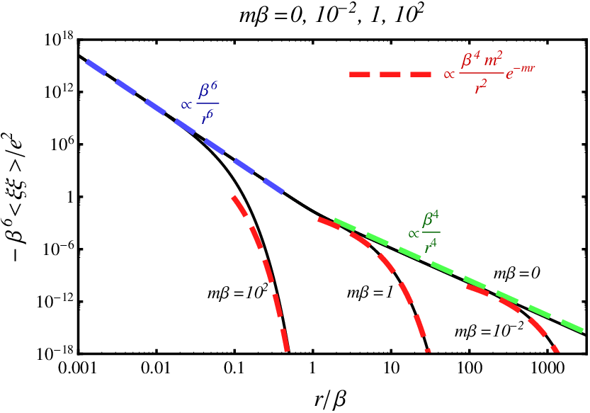
Refer to caption
Figure 2: Noise spatial correlations for various mass values. The solid black line represents the exact expression (45) with Eqs. (49) ∼\sim (53). The dashed blue, red, and green lines correspond to the analytical approximations (54), (56), and (57). For r<1mr<\frac{1}{m}, correlations obey power-law decay. They start to decay exponentially when rr exceeds 1m\frac{1}{m}.

We show the spatial correlation for various masses in FIG. 2. As the approximate expression (56) shows, the noise correlation is exponentially suppressed at r∼>1mr\raisebox{-2.15277pt}{$\>\stackrel{{\scriptstyle\textstyle>}}{{\sim}}\>$}\frac{1}{m} and monotonically approaches zero. Asymptotically, the noise correlation obtained by numerical evaluation is consistent with the above simple expressions obtained analytically. We see that the noise in this model shows anti-correlation, which is different from the previous study [14].

III.4 Dissipation rate

The Langevin equation provides not only fluctuations to the scalar field but also its dissipation.

According to Ref. [15, 23], for the scalar field described by the equation

(−ω2+Mk,ω2)​ϕ~​(ω,k→)+12​C~​(ω,k→)​ϕ~​(ω,k→)=ξ~​(ω,k→),(-\omega^{2}+M_{k,\omega}^{2})\tilde{\phi}(\omega,\vec{k})+\frac{1}{2}\tilde{C}(\omega,\vec{k})\tilde{\phi}(\omega,\vec{k})=\tilde{\xi}(\omega,\vec{k})\,, (58)

the dissipation rate of the kk-mode oscillation is given by

ΓD(k→)=−ImC~(k→,Mk,ω)/2Mk,ω.\Gamma_{\rm D}(\vec{k})=-{\rm Im}\tilde{C}(\vec{k},M_{k,\omega})/2M_{k,\omega}\,. (59)

This expression is valid if the ω\omega and nontrivial kk-dependence of Mk,ωM_{k,\omega} is negligibly small, that is

Mk,ω2=k2+M02,M_{k,\omega}^{2}=k^{2}+M^{2}_{0}\,, (60)

where M0M_{0} is a constant. In this study, Mk,ωM_{k,\omega} is given by

Mk,ω2=k2+m2+e2​T26−f~A0​(ω,k→)+∫d​ω′2​π​P​1ω−ω′​i​C~k→​(ω′).M^{2}_{k,\omega}=k^{2}+m^{2}+e^{2}\frac{T^{2}}{6}-\tilde{f}_{A_{0}}(\omega,\vec{k})+\int\frac{d\omega^{\prime}}{2\pi}{\rm P}\frac{1}{\omega-\omega^{\prime}}i\tilde{C}_{\vec{k}}(\omega^{\prime})\,. (61)

Both f~A0\tilde{f}_{A_{0}} and the principal value integral are divergent. In Appendix C, we show this divergence can be removed by renormalizing the scalar field strength. In other words, we can cancel out this divergence by the counter term which is proportional to the kinetic term of the scalar field. Although the kk and ω\omega-dependence of Mk,ωM_{k,\omega} are non-trivial, such corrections are proportional to e2e^{2}. If we assume Mk,ωM_{k,\omega} is given by Eq. (60), we find

ΓD​(k→)=\displaystyle\Gamma_{\rm D}(\vec{k})= e24​π​kM02+k2​∫pipfd​p​(1+1eβ​p−1−1eβ⁡(M02+k2−p)−1)\displaystyle\frac{e^{2}}{4\pi}\frac{k}{\sqrt{M^{2}_{0}+k^{2}}}\int^{p_{f}}_{p_{i}}dp\left(1+\frac{1}{e^{\beta p}-1}-\frac{1}{e^{\beta(\sqrt{M^{2}_{0}+k^{2}}-p)}-1}\right)
×[−M02k2+(M02−m2)​M02+k2k2​p−(M02−m2)24​k2​p2]\displaystyle\qquad\qquad\times\left[-\frac{M^{2}_{0}}{k^{2}}+\frac{(M^{2}_{0}-m^{2})\sqrt{M^{2}_{0}+k^{2}}}{k^{2}p}-\frac{(M^{2}_{0}-m^{2})^{2}}{4k^{2}p^{2}}\right] (62)
pi=\displaystyle p_{i}= M02−m22​(M02+k2+k),pf=M02−m22​(M02+k2−k)\displaystyle\frac{M^{2}_{0}-m^{2}}{2(\sqrt{M^{2}_{0}+k^{2}}+k)}\,,\quad p_{f}=\frac{M^{2}_{0}-m^{2}}{2(\sqrt{M^{2}_{0}+k^{2}}-k)}

Though we have assumed M0>mM_{0}>m in deriving the above expression, it is finite even in taking M0→mM_{0}\rightarrow m. In this limit, we can obtain

ΓD​(k→)={e23​π​β​k2m2k≪me22​π​βk≫m.\Gamma_{\rm D}(\vec{k})=\left\{\begin{array}[]{ll}\frac{e^{2}}{3\pi\beta}\frac{k^{2}}{m^{2}}&k\ll m\\ \frac{e^{2}}{2\pi\beta}&k\gg m\,.\end{array}\right. (63)

We show the dissipation rate as a function of kk in FIG. 3 for various values of β​m\beta m *4*4 *4 Note that we should not take the high-temperature limit (β​m→0\beta m\rightarrow 0) for the result in FIG. 3, since in such a case the difference between M0M_{0} and mm is not negligible..

Refer to caption
Figure 3: The kk-dependence of the dissipation rate (62). The dashed black line represents β​ΓD=e2/2​π\beta\Gamma_{\rm D}=e^{2}/2\pi. The red, green, blue line represents the dissipation rate for β​m=10−2, 1, 102\beta m=10^{-2},\,1,\,10^{2}, respectively. For k>mk>m, the dissipation rate is almost independent of kk. However, for k<mk<m, it is proportional to k2k^{2}.

Since both the dissipation and fluctuation come from the left diagram in FIG.1, we can see the physical processes related to dissipation and fluctuation by cutting the diagram into two pieces [24]. Considering the fact that a scalar boson cannot decay into a scalar boson of the same species and a massless gauge boson due to energy and momentum conservation, it may be doubtful that Eq.(62) is the physical dissipation rate. Though the dissipation rate shown in FIG.3 is expressed as an integral over the loop momentum, only the p→=0→\vec{p}=\vec{0}, or a soft photon loop, contributes to the resultant finite value. From a mathematical point of view, it results from a cancellation between the divergent contribution from the bosonic distribution function and the vanishment of the phase space. In order to see whether this finite result due to the aforementioned cancellation is physically relevant, we have considered the same problem in a finite box having a spatial volume VV with a periodic boundary condition where momentum is discretized and the zero-mode contribution is isolated. It is found that the zero-mode contribution contains the thermal average of the field value squared which evidently diverges since no particular field value is energetically favored. As a result, contribution to Eq.(62) scales as ΦΛ2/V\Phi_{\Lambda}^{2}/V, where ΦΛ\Phi_{\Lambda} is a cutoff of the zero-mode field amplitude. Thus, the zero-mode contribution has an ambiguity arising from its dependence on the order of taking the limit ΦΛ→∞\Phi_{\Lambda}\to\infty and V→∞V\to\infty. Hence we may not trust the finite value obtained in Eq.(62) which is based on the particular continuum calculation. Indeed the Eq.(62) itself would vanish if, we incorporate a plasmon mass to the gauge field using a dressed propagator, or simply a mass term generated by a finite value of ϕ\phi. In this case Eq.(33) would also vanish, as it should.

Thus the dissipation arises from diagrams higher order in ee as shown in FIG. 4 related to the interaction e2​Aμ​Aμ​Φ†​Φe^{2}A_{\mu}A^{\mu}\Phi^{\dagger}\Phi. In this case, the noise becomes the multiplicative noise, which appears in the equation of motion of ϕ\phi in a form like ξ​ϕ\xi\,\phi. The non-local memory term in the effective action is

Γ⊃\displaystyle\Gamma\supset −4ie4∫d4x1d4x2[ϕcR(x1)ϕΔ​R(x1)+ϕcI(x1)ϕΔ​I(x1)][|ϕc(x2)|2+14|ϕΔ(x2)|2]\displaystyle-4ie^{4}\int d^{4}x_{1}d^{4}x_{2}\left[\phi_{\rm cR}(x_{1})\phi_{\rm\Delta R}(x_{1})+\phi_{\rm cI}(x_{1})\phi_{\rm\Delta I}(x_{1})\right]\left[|\phi_{\rm c}(x_{2})|^{2}+\frac{1}{4}|\phi_{\rm\Delta}(x_{2})|^{2}\right]
×∫d3​k1(2​π)3d3​k2(2​π)3e−i(k1→+k2→)⋅(x1→−x2→)𝒫i​j(k1→)𝒫i​j(k2→)\displaystyle\quad\times\int\frac{d^{3}k_{1}}{(2\pi)^{3}}\frac{d^{3}k_{2}}{(2\pi)^{3}}e^{-i(\vec{k_{1}}+\vec{k_{2}})\cdot(\vec{x_{1}}-\vec{x_{2}})}{\cal P}_{ij}(\vec{k_{1}}){\cal P}_{ij}(\vec{k_{2}})
[gk1>​(t1,t2)​gk2>​(t1,t2)−gk1<​(t1,t2)​gk2<​(t1,t2)]​Θ​(t1−t2).\displaystyle\qquad\quad\left[g^{>}_{k_{1}}(t_{1},t_{2})g^{>}_{k_{2}}(t_{1},t_{2})-g^{<}_{k_{1}}(t_{1},t_{2})g^{<}_{k_{2}}(t_{1},t_{2})\right]\Theta(t_{1}-t_{2})\,. (64)

The dissipation rate corresponding to multiplicative noise cases is also studied in Ref. [15]. Using the following quantity

Cm​(x−x′)≡\displaystyle C_{\rm m}(x-x^{\prime})\equiv 4ie4∫d3​k1(2​π)3d3​k2(2​π)3e−i(k1→+k2→)⋅(x→−x′→)𝒫i​j(k1→)𝒫i​j(k2→)\displaystyle 4ie^{4}\int\frac{d^{3}k_{1}}{(2\pi)^{3}}\frac{d^{3}k_{2}}{(2\pi)^{3}}e^{-i(\vec{k_{1}}+\vec{k_{2}})\cdot(\vec{x}-\vec{x^{\prime}})}{\cal P}_{ij}(\vec{k_{1}}){\cal P}_{ij}(\vec{k_{2}})
[gk1>​(t,t′)​gk2>​(t,t′)−gk1<​(t,t′)​gk2<​(t,t′)],\displaystyle\left[g^{>}_{k_{1}}(t,t^{\prime})g^{>}_{k_{2}}(t,t^{\prime})-g^{<}_{k_{1}}(t,t^{\prime})g^{<}_{k_{2}}(t,t^{\prime})\right]\,, (65)

we can evaluate the dissipation rate for the homogeneous field as

ΓD=C~m​(k→=0→,2​M)2​i​M​|ϕ⁡(t)|2=e4​|ϕ⁡(t)|24​π​M​(1+2​NM).\Gamma_{\rm D}=\frac{\tilde{C}_{\rm m}(\vec{k}=\vec{0},2M)}{2iM}|\phi(t)|^{2}=\frac{e^{4}|\phi(t)|^{2}}{4\pi M}(1+2N_{M})\,. (66)

Here MM is the angular frequency of the coherent oscillation and |ϕ⁡(t)|2|\phi(t)|^{2} is a mean square amplitude around the time tt. So even the coherent oscillation has nonzero dissipation at this order.

Refer to caption
Figure 4: 1PI diagram relevant to the multiplicative noise. This 𝒪⁡(e4){\mathcal{O}(e^{4})} diagram leads to the nonzero dissipation rate for the coherently oscillating scalar field.

IV Summary

In this paper, we studied the role of gauge fields in the effective action for the scalar field by considering the scalar QED theory. As can be expected from previous studies, the effective action we obtained contains an imaginary part. We rewrote it by applying the Gaussian functional integral formula, and interpreted the integral over variable ξ\xi as ensemble averaging. The validity of this arrangement is confirmed by the fluctuation-dissipation relation between the memory term and the introduced noise term. Then we analyzed the spatial correlation of the noise, and found the noise shows anti-correlation, which is different from the case of scalar and fermionic interactions. The origin of this anti-correlation is due to the existence of derivative interactions between the scalar and gauge field. We also considered the dissipation rate of the scalar field. Though we obtained a finite dissipation rate, it comes from a soft photon in the loop. It would vanish if we incorporate a finite mass which may be generated from higher order loops. Furthermore since the dissipation we have obtained comes from derivative interactions, the dissipation rate for the coherent oscillation vanishes. On the other hand higher order diagrams, consisting of a non-derivative interaction as depicted in FIG.4, gives a nonzero dissipation rate.

Considering that gauge coupling constants are generally larger than Yukawa coupling constants, the absolute value of the noise correlation function for massless case (Eqs. (54) and (57)) can be larger than that of fermionic noise studied by Ref. [14]. It would be interesting to study the phase transitions numerically with our results included. One of the other future works is to extend this study to non-Abelian gauge theories in order to treat the realistic phenomena in the early Universe.

Acknowledgments

We would like to thank Marco Drewes for helpful comments. This work was supported by JSPS Research Fellowships for Young Scientists (Y.M.), the Grant-in-Aid for Scientific Research on Innovative Areas No. 25103505 (T.S.), No. 24103006 (H.M.), No. 21111006 (J.Y.), No. 25103504 (J.Y.) from The Ministry of Education, Culture, Sports, Science and Technology (MEXT), and JSPS Grant-in-Aid for Scientific Research No. 23340058 (J.Y.).

Appendix A: short-range noise correlation

From (49)∼\sim(53), we obtain the following asymptotic form as r→0r\rightarrow 0.

α⁡(r)\displaystyle\alpha(r) →12​π2​r2\displaystyle\rightarrow\frac{1}{2\pi^{2}r^{2}}
β′​(r)\displaystyle\beta^{\prime}(r) →−12​π2​r,β′′​(r)→12​π2​r2\displaystyle\rightarrow-\frac{1}{2\pi^{2}r}\,,\qquad\beta^{\prime\prime}(r)\rightarrow\frac{1}{2\pi^{2}r^{2}}
γ′​(r)\displaystyle\gamma^{\prime}(r) →−1π2​r3,γ′′​(r)→3π2​r4\displaystyle\rightarrow-\frac{1}{\pi^{2}r^{3}}\,,\qquad\gamma^{\prime\prime}(r)\rightarrow\frac{3}{\pi^{2}r^{4}} (67)

To derive these results, we have used the fact that modified Bessel functions Kn​(x)K_{n}(x) satisfy

limx→0xn​Kn​(x)=2−1+n​Γ​(n).\lim_{x\rightarrow 0}x^{n}K_{n}(x)=2^{-1+n}\Gamma(n)\,. (68)

Using the above expressions, the spatial noise correlation becomes

⟨ξ⁡(x1→,t)​ξ†​(x2→,t)⟩≃−3​e22​π4​r6,\langle\xi(\vec{x_{1}},t)\xi^{\dagger}(\vec{x_{2}},t)\rangle\,\simeq\,-\frac{3e^{2}}{2\pi^{4}r^{6}}\,, (69)

as rr approaches zero.

Since the value at r=0r=0 corresponds to ⟨|ξ⁡(x→,t)|2⟩\langle|\xi(\vec{x},t)|^{2}\rangle, the correlation function given by Eq. (69) being negative seems strange. We speculate that the origin of this apparent contradiction lies in the evaluation of γi​j\gamma_{ij}. To see the essence, we now consider the case where the scalar field is massless.

The divergence comes from the zero-temperature part.

γzero′\displaystyle\gamma^{\prime}_{\rm zero} =12​π2​∫0∞d​p​(p​cos⁡(p​r)r−sin⁡(p​r)r2)\displaystyle=\frac{1}{2\pi^{2}}\int_{0}^{\infty}dp\left(\frac{p\cos(pr)}{r}-\frac{\sin(pr)}{r^{2}}\right) (70)
γzero′′\displaystyle\gamma^{\prime\prime}_{\rm zero} =12​π2​∫0∞d​p​(−p2​sin⁡(p​r)r−2​p​cos⁡(p​r)r2+2​sin⁡(p​r)r3)\displaystyle=\frac{1}{2\pi^{2}}\int_{0}^{\infty}dp\left(\frac{-p^{2}\sin(pr)}{r}-2\frac{p\cos(pr)}{r^{2}}+2\frac{\sin(pr)}{r^{3}}\right) (71)

These integrals are UV divergent. We regulate them by introducing a cutoff factor e−p/Λe^{-p/\Lambda}, getting

γzero′\displaystyle\gamma^{\prime}_{\rm zero} =−12​π2​2​r​Λ4(1+r2​Λ2)2,\displaystyle=-\frac{1}{2\pi^{2}}\frac{2r\Lambda^{4}}{(1+r^{2}\Lambda^{2})^{2}}\,, (72)
γzero′′\displaystyle\gamma^{\prime\prime}_{\rm zero} =12​π2​2​Λ4​(3​r2​Λ2−1)(1+r2​Λ2)3.\displaystyle=\frac{1}{2\pi^{2}}\frac{2\Lambda^{4}(3r^{2}\Lambda^{2}-1)}{(1+r^{2}\Lambda^{2})^{3}}\,. (73)

If we evaluate the noise correlation with these regulated integral, the asymptotic form becomes

⟨ξ⁡(x1→,t)​ξ†​(x2→,t)⟩≃−e22​π4​Λ4​(3​r2​Λ2−1)r2​(1+r2​Λ2)3.\langle\xi(\vec{x_{1}},t)\xi^{\dagger}(\vec{x_{2}},t)\rangle\,\simeq\,-\frac{e^{2}}{2\pi^{4}}\frac{\Lambda^{4}(3r^{2}\Lambda^{2}-1)}{r^{2}(1+r^{2}\Lambda^{2})^{3}}\,. (74)

When r>0r>0, taking Λ→∞\Lambda\rightarrow\infty gives the same result as (69). On the other hand, if we keep Λ\Lambda finite and take r→+0r\rightarrow+0, we see that the spatial noise correlation goes to +∞+\infty. At r=0r=0, the dominant part is e22​π4​Λ4r2​(1+r2​Λ2)3\frac{e^{2}}{2\pi^{4}}\frac{\Lambda^{4}}{r^{2}(1+r^{2}\Lambda^{2})^{3}}. If we multiply it by r5r^{5} and integrate from 00 to ∞\infty, we obtain a finite value.

∫0∞d​r​Λ4r2​(1+r2​Λ2)3×r5=14\int_{0}^{\infty}dr\,\frac{\Lambda^{4}}{r^{2}(1+r^{2}\Lambda^{2})^{3}}\times r^{5}=\frac{1}{4} (75)

From this, we can write as follows.

e22​π4​Λ4r2​(1+r2​Λ2)3=e24​π4​r5​δ​(r)\frac{e^{2}}{2\pi^{4}}\frac{\Lambda^{4}}{r^{2}(1+r^{2}\Lambda^{2})^{3}}=\frac{e^{2}}{4\pi^{4}r^{5}}\delta(r) (76)

Appendix B: long-range noise correlation

We briefly show the long-range (r≫β,1mr\gg\beta,\,\frac{1}{m}) behavior. In this limit, we obtain

α⁡(r)\displaystyle\alpha(r) →12​π​β​r\displaystyle\rightarrow\frac{1}{2\pi\beta r}
β′​(r)\displaystyle\beta^{\prime}(r) →−14​π​β\displaystyle\rightarrow-\frac{1}{4\pi\beta}
β′′​(r)\displaystyle\beta^{\prime\prime}(r) →β12​π​r3\displaystyle\rightarrow\frac{\beta}{12\pi r^{3}}
γ′​(r)\displaystyle\gamma^{\prime}(r) →{−12​π​β​r2m=0−m2​π​r​β​e−m​rm≠0\displaystyle\rightarrow\left\{\begin{array}[]{ll}-\frac{1}{2\pi\beta r^{2}}&m=0\\ -\frac{m}{2\pi r\beta}e^{-mr}&m\neq 0\end{array}\right.
γ′′​(r)\displaystyle\gamma^{\prime\prime}(r) →{1π​β​r3m=0m22​π​r​β​e−m​rm≠0\displaystyle\rightarrow\left\{\begin{array}[]{ll}\frac{1}{\pi\beta r^{3}}&m=0\\ \frac{m^{2}}{2\pi r\beta}e^{-mr}&m\neq 0\end{array}\right.

In the evaluation of γ′\gamma^{\prime} and γ′′\gamma^{\prime\prime}, we used the asymptotic form for modified Bessel functions Kn​(x)K_{n}(x),

Kn(x)→π2x−1/2e−xasx→∞.K_{n}(x)\rightarrow\sqrt{\frac{\pi}{2}}x^{-1/2}e^{-x}\quad{\rm as}\,\,x\rightarrow\infty. (81)

Appendix C: scalar field strength renormalization

We show the divergent part of

−f~A0​(ω,k→)+∫d​ω′2​π​P​1ω−ω′​i​C~k→​(ω′)-\tilde{f}_{A_{0}}(\omega,\vec{k})+\int\frac{d\omega^{\prime}}{2\pi}{\rm P}\frac{1}{\omega-\omega^{\prime}}i\tilde{C}_{\vec{k}}(\omega^{\prime}) (82)

can be removed by renormalizing the field strength of the scalar field.

First, f~A0\tilde{f}_{A_{0}} can be expressed as

−f~A0​(ω,k→)=e22​∫d3​q(2​π)3​ω2+ωq2ωq​|k→−q→|2​(1+2​nq).-\tilde{f}_{A_{0}}(\omega,\vec{k})=\frac{e^{2}}{2}\int\frac{d^{3}q}{(2\pi)^{3}}\frac{\omega^{2}+\omega_{q}^{2}}{\omega_{q}|\vec{k}-\vec{q}|^{2}}(1+2n_{q})\,. (83)

This is an UV-divergent integral, whose divergence comes from zero temperature part. Sticking to massless case which does not loss generality of the analysis in this section, we find

−f~A0​(ω,k→)→e216​π2​k​∫0∞d​q​(ω2+q2)​ln⁡(k+q)2(k−q)2.-\tilde{f}_{A_{0}}(\omega,\vec{k})\rightarrow\frac{e^{2}}{16\pi^{2}k}\int_{0}^{\infty}dq(\omega^{2}+q^{2})\ln\frac{(k+q)^{2}}{(k-q)^{2}}\,. (84)

Now we use the dimensional regularization method. Changing the dimensions from 33 to 3+ϵ3+\epsilon in Eq. (83) enables us to extract the divergence as follows.

−f~A0​(ω,k→)=e212​π2​(3​ω2+k2)​1ϵ+(regular​terms)-\tilde{f}_{A_{0}}(\omega,\vec{k})=\frac{e^{2}}{12\pi^{2}}(3\omega^{2}+k^{2})\frac{1}{\epsilon}+({\rm regular\,\,terms}) (85)

Second, it is convenient to use another expression for the principal integral term,

∫d​ω′2​π​P​1ω−ω′​i​C~k→​(ω′)\displaystyle\quad\int\frac{d\omega^{\prime}}{2\pi}{\rm P}\frac{1}{\omega-\omega^{\prime}}i\tilde{C}_{\vec{k}}(\omega^{\prime})
=−e22∫d3​p(2​π)3𝒫i​jkikj1p​ωk+p\displaystyle=-\frac{e^{2}}{2}\int\frac{d^{3}p}{(2\pi)^{3}}{\cal P}_{ij}k_{i}k_{j}\frac{1}{p\,\omega_{k+p}}
×[(1+2Np)(Pω+p+ωk+p−Pω−p−ωk+p−Pω+p−ωk+p+Pω−p+ωk+p)\displaystyle\quad\times\Bigg[(1+2N_{p})\left(\frac{\rm P}{\omega+p+\omega_{k+p}}-\frac{\rm P}{\omega-p-\omega_{k+p}}-\frac{\rm P}{\omega+p-\omega_{k+p}}+\frac{\rm P}{\omega-p+\omega_{k+p}}\right)
+(1+2nk+p)(Pω+p+ωk+p−Pω−p−ωk+p−Pω−p+ωk+p+Pω+p−ωk+p)].\displaystyle\qquad+(1+2n_{k+p})\left(\frac{\rm P}{\omega+p+\omega_{k+p}}-\frac{\rm P}{\omega-p-\omega_{k+p}}-\frac{\rm P}{\omega-p+\omega_{k+p}}+\frac{\rm P}{\omega+p-\omega_{k+p}}\right)\Bigg]\,. (86)

This is also UV divergent and we use the dimensional regularization method once more. The above integral at large pp is simplified to

−e2​k23​π∫∞dpp−1+ϵ→−e2​k23​π21ϵ.-\frac{e^{2}k^{2}}{3\pi}\int^{\infty}dp\,p^{-1+\epsilon}\rightarrow-\frac{e^{2}k^{2}}{3\pi^{2}}\frac{1}{\epsilon}\,. (87)

Finally we find Eq.(82) diverges like e24​π2​(ω2−k2)​1ϵ\frac{e^{2}}{4\pi^{2}}(\omega^{2}-k^{2})\frac{1}{\epsilon}. This combination of (ω2−k2)(\omega^{2}-k^{2}) ensures that we can remove this divergence by the renormalization of the scalar field strength.

References

  • [1] P. A. R. Ade et al. [Planck Collaboration], arXiv:1303.5076 [astro-ph.CO].
  • [2] A. A. Starobinsky, Phys. Lett. B 91, 99 (1980).
  • [3] A. H. Guth, Phys. Rev. D 23, 347 (1981).
  • [4] K. Sato, Mon. Not. Roy. Astron. Soc. 195, 467 (1981).
  • [5] A. D. Linde, Phys. Lett. B 108, 389 (1982).
  • [6] A. Albrecht and P. J. Steinhardt, Phys. Rev. Lett. 48, 1220 (1982).
  • [7] A. D. Linde, Phys. Lett. B 129, 177 (1983).
  • [8] D. H. Lyth and E. D. Stewart, Phys. Rev. D 53, 1784 (1996) [hep-ph/9510204].
  • [9] R. Easther, J. T. Giblin, Jr., E. A. Lim, W. -I. Park and E. D. Stewart, JCAP 0805, 013 (2008) [arXiv:0801.4197 [astro-ph]].
  • [10] M. Kamionkowski, A. Kosowsky and M. S. Turner, Phys. Rev. D 49, 2837 (1994) [astro-ph/9310044].
  • [11] T. Vachaspati and A. Vilenkin, Phys. Rev. D 31, 3052 (1985); T. Damour and A. Vilenkin, Phys. Rev. D 71, 063510 (2005) [hep-th/0410222].
  • [12] S. Kuroyanagi, K. Miyamoto, T. Sekiguchi, K. Takahashi and J. Silk, Phys. Rev. D 86, 023503 (2012) [arXiv:1202.3032 [astro-ph.CO]]; M. R. DePies and C. J. Hogan, Phys. Rev. D 75, 125006 (2007) [astro-ph/0702335].
  • [13] M. Morikawa, Phys. Rev. D 33, 3607 (1986); M. Gleiser and R. O. Ramos, Phys. Rev. D 50, 2441 (1994) [hep-ph/9311278].
  • [14] M. Yamaguchi and J. Yokoyama, Phys. Rev. D 56, 4544 (1997) [hep-ph/9707502].
  • [15] J. Yokoyama, Phys. Rev. D 70, 103511 (2004) [hep-ph/0406072].
  • [16] S. -Y. Wang, D. Boyanovsky, H. J. de Vega and D. S. Lee, Phys. Rev. D 62, 105026 (2000) [hep-ph/0005223]; D. Boyanovsky, H. J. de Vega and M. Simionato, Phys. Rev. D 61, 085007 (2000) [hep-ph/9909259].
  • [17] D. Boyanovsky, H. J. de Vega, R. Holman, S. P. Kumar and R. D. Pisarski, Phys. Rev. D 58, 125009 (1998) [hep-ph/9802370].
  • [18] M. Le Bellac, Thermal Field Theory (Cambridge University Press, Cambridge, England, 1996).
  • [19] N. P. Landsman and C. G. van Weert, Phys. Rept. 145, 141 (1987).
  • [20] E. Calzetta and B. L. Hu, Phys. Rev. D 61, 025012 (2000) [hep-ph/9903291].
  • [21] E. Calzetta and B. L. Hu, Nonequilibrium Quantum Field Theory (Cambridge University Press, Cambridge, England, 2008).
  • [22] A. Berera, I. G. Moss and R. O. Ramos, Phys. Rev. D 76, 083520 (2007) [arXiv:0706.2793 [hep-ph]].
  • [23] C. Greiner and B. Muller, Phys. Rev. D 55, 1026 (1997) [hep-th/9605048].
  • [24] M. Drewes and J. U. Kang, Nucl. Phys. B 875, 315 (2013) [arXiv:1305.0267 [hep-ph]].