Almost Optimal Channel Access in Multi-Hop Networks With Unknown Channel Variables
Abstract
We consider distributed channel access in multi-hop cognitive radio networks. Previous works on opportunistic channel access using multi-armed bandits (MAB) mainly focus on single-hop networks that assume complete conflicts among all secondary users. In the multi-hop multi-channel network settings studied here, there is more general competition among different communication pairs. We formulate the problem as a linearly combinatorial MAB problem that involves a maximum weighted independent set (MWIS) problem with unknown weights which need to learn. Existing methods for MAB where each of nodes chooses from channels have exponential time and space complexity , and poor theoretical guarantee on throughput performance. We propose a distributed channel access algorithm that can achieve of the optimum averaged throughput where each node has communication complexity and space complexity in the learning process, and time complexity in strategy decision process for an arbitrary wireless network. Here is the approximation ratio to MWIS for a local -hop network with nodes, and is the number of mini-rounds inside each round of strategy decision. For randomly located networks with an average degree , the time complexity is .
I Introduction
Available spectrum is being exhausted, while a lot of frequency bands are extremely under utilized. As a promising solution to improve dynamic allocation of the under-utilized spectrum, cognitive radio technology allows secondary users to opportunistically access vacant channels in temporal and spatial domain when the primary user is idle. However, due to resource and hardware constraints, at a given time, cognitive radios (CR) can sense only a part of heterogeneous channels with unknown quality before transmission.
Thus, it is core for secondary users to learn and select the best possible channels to access. Several recent results [1], [2], [3], [4], [5], [6], [7] are proposed to take the dynamic spectrum sharing problem as the multi-armed bandits problem, and attempt to find a dynamic channel access policy that results in almost optimal expected throughput (or zero-regret) through learning history, compared with the optimal fixed channel policy. However, these methods generally adopt the simplest form of MAB where only single-hop networks fit the model. Dynamic channel access in multihop cognitive radio networks demands more sophisticated formulation that considers constraints of general interference among users. A naive extension of formulation from the single-hop case to multihop case will lead to regret, time and space complexity that is exponential with the number of users in the learning process. More specifically, taken as an arm a strategy consisting of decisions from each of the users, there will be combinations totally when each user has channels to choose. As all these aforementioned works adopt a UCB-type learning policy [8] [9] [10], the upper bound of regret as well as time and space complexity is linear with the number of arms, thus linear with in multihop networks.
Efficient channel access under multihop networks also requires decentralized design with low computation and communication. Previous decentralized MAB methods [4] [2] [11] pay little attention to these practical challenges around multihop networks. Though there is no communication cost in [4][2], they require exponential time in a single learning round. Distinct from [4], [2] assumes multiple users can access the same resource, which does not capture conflicts among near-by users. On the other hand, [12] proposes a low-computation learning policy for multi-hop networks, but the policy takes a centralized form and still leaves challenges on distributed implementation unsolved.
Here we investigate the problem of achieving maximum expected throughput through a decentralized learning process with low computation and communication cost. As this problem involves competition among adjacent users, and cooperation for maximum throughput network wide, there may be no effective solutions if we directly formulate the problem into an integer linear programming. We then subtly formulate the problem into a linearly combinatorial MAB problem that shall find a maximum weighted independent set of vertexes where weight is unknown channel quality. This novel formulation facilitates us to utilize a zero-regret learning policy where it only costs time and space complexity for a network with channels and secondary users. The other benefit is that we can adaptively choose efficient methods to solve the involved NP-hard MWIS problem and still achieve zero-regret.
We propose a decentralized channel access scheme based on robust PTAS [13] to approximately solve the MWIS problem. Our decentralized implementation achieves an approximation ratio of , but only requires time complexity to find the strategy decision after weight is estimated. Here is the hop number required to achieve a robust PTAS[13], which is a constant for networks with a constant number of channels to choose. It costs time complexity for a random network. Our simulation results show that our new distributed learning policy indeed outperforms previous policies in terms of average throughput, time and storage cost.
II Network model
Consider a network with a set of nodes (users), a set of edges denoting conflicts, and a set of channels. We assume is a constant as the number of available frequency bands is fixed in a given network. We use unit disks to model conflicts between two nodes, where each node is treated as a disk centered on itself. Conflicts happen if any two intersected disks access the same channel simultaneously. The network is time-slotted with global synchronization. At each round , node has choices of channels, where channel having data rate drawn from an i.i.d stochastic process over time with a mean . Without loss of generality, we assume the same channel may demonstrate different channel quality for different users. For the same channel , the random process is independent from if .
At each round , an -dimensional strategy vector is selected under some policy from the feasible strategy set . Here is the index of channel selected by node in strategy . We use to index strategies of feasible set in the decreasing order of average throughput . By feasible we mean that all nodes can transmit simultaneously without conflict. When a strategy is determined, each node observes the data rate of its selected channel, and then the total throughput of the network at is defined as, We evaluate policies using regret, which is defined as the difference between the expected throughput that could be obtained by a static optimal policy with the existence of a genie, and that obtained by the given policy. Let be the optimum fixed channel access strategy, then regret can be expressed as
| (1) |
III Problem formulation
| Variable | Meaning |
|---|---|
| -hop neighborhood of node in | |
| -hop neighborhood of vertex in | |
| set of Candidate vertexes in -hop neighborhood of | |
| maximum weighted independent set for vertex set | |
| independent set with maximum cardinality for vertex set | |
| summed weight of all vertexes in vertex set | |
| strategy decision for round |
We first analyze the optimum throughput on the assumption that the mean of each random variable is known. We remodel the network as an extended conflict graph , where , and show that the problem can be reformulated as a MWIS problem in extended conflict graph . Define a set of virtual vertices , for each node and connect with for all . Node is master node of virtual vertex , while is slave of . Connect with if and has an edge in original network . Then graph has vertexes. We give an instance in Fig. 1 where the original network has available channels and nodes.

As each node of has a clique of virtual vertexes in , and vertexes with the same channel index retain the conflict relationships of master nodes in , then it is straightforward that a MWIS of is a throughput-optimal allocation of channels in . Indeed, an IS of one-to-one maps to a feasible strategy in . Therefore, the feasible strategy set consists of all independent sets (IS) of vertexes in . Here note that the independence number of is less than if the chromatic number of is greater than , and is otherwise. The actual length of a feasible strategy may be smaller than if some nodes do not choose any channel. Let be weight of virtual vertex . If the mean of is known, the optimum strategy is to find a maximum weighted independent set of vertexes from as choices made by nodes in , i.e,
| (2) |
However, these random variables are unknown actually, each user needs to learn and estimate the weight of each strategy, denoted by , where is estimated weight of random variable . Thus, our problem becomes a NP-hard combinatorial multi-armed bandits problem that selects at most arms (i.e., vertexes in ) out of ones to minimize the regret , such that these arms are independent from each other in . For brevity, we map the channel index of node to arm index .
For NP-hard combinatorial multi-armed bandits problems, a weaker vision of regret, called -regret [14], is defined as the difference between the expected throughput that is of the optimum, and that gained throughput (a -approximation policy which instead yields a strategy with learned weight at least of the maximum possible weight) . Let be the reward of strategy generated by the -approximation policy, then -regret can be expressed as
where is the number of times that strategy has been played by round , and is the distance between and mean throughput of strategy .
Though a previous learning policy in [11] achieves zero-regret, the upper bound of regret heavily depends on the distribution of strategies in feasible set (or which is all strategies whose throughput is at least ). That is, the upper bound of regret (or -regret ) including a factor of (or ) becomes vacuous if (or ) . We expect a zero-regret policy without dependency on . Meanwhile, it admits distributed implementation with low computation and communication complexity to guarantee efficiency of the channel access process.
IV Channel access
Each round is divided into two sequent parts, one for strategy decision and the other for data transmission. In the strategy decision part, it utilizes the learned information in history to determine which strategy shall be selected for current time. In the data transmission part, users access corresponding channels to transmit data, and observe real data rate after transmission. We assume a common control channel for control message passing in strategy decision.
IV-A The learning policy
To learn for the best possible strategy, we adopt the learning policy proposed in [14] where the upper bound of regret is independent with (or ). The centralized form of the learning policy is shown in Algorithm 1, where in (4) it utilizes estimated weight of each vertex in to select a maximum weighted independent set as strategy decision for next channel access. The estimated value for actual weight of vertex is
| (3) |
| (4) |
Consequently, it only requires to store and update estimation for vertexes that costs storage and computation linear with , instead for strategies in that costs storage and computation linear with . More specially, we need two vectors to store and update the estimated weight. One is where is observed mean of up to the current round, and the other is where is the number of times that channel has been selected so far. After data transmission on the channels of chosen strategy in slot , actual weight is observed for all . Then and are updated in the following way:
Due to NP-hardness of the MWIS problem in (4), it is desirable to solve it approximately while retaining zero-regret. The following theorem shows that, for any algorithm with approximation ratio at least for the MWIS problem, the regret on the achieved throughput is bounded.
Theorem 1
[14] The -approximation learning policy has
| (11) | |||||
without dependency on . The supremum is taken over all -tuple of probability distributions on .
IV-B Centralized approximation solution for channel access
Intuitively, the greater the value is, the more sacrifice on overall throughput it causes. Given that, we choose the robust PTAS proposed in [13] to solve the MWIS problem. Though centralized, the robust PTAS is elegant, and more importantly, it requires no geometric information as other PTAS schemes [15] [16]. This feature is very attractive as it is expensive to get and maintain exact locations of each node in multi-hop wireless networks, not to say negative effect of errors by location methods. We will show how to implement it in a distributed manner later. For better understanding, we first introduce the centralized method.
Robust PTAS. We begin with some notations. Given a unit disk graph with a set of nodes and a set of edges, an edge if the Euclidean distance . For a subset of nodes in , let denote the total weight of , i.e., , and denote a maximum weighted independent set for . The independent set with maximal cardinality (MIS) for is written as . Let be the minimum hop of any path connecting and in . Define
be the -hop neighborhood of in . The -hop distance of , is the maximum Euclidean distance between and neighbors in . Clearly .
Let and denote the desired approximation guarantee. In graph , the algorithm starts with a node of maximal weight , and then computes as long as holds. Let denote the smallest for which the criterion is violated. It has been proved that is a constant for a specific , i.e., . We then remove and all the adjacent vertices from , and repeat the above process on the remaining graph. Then the union of all removed independent sets form an independent set, and it is proved that it is -approximation for the MWIS of unit disk graph .
As the extended conflict graph is not a strict unit disk graph, we distinguish some notations. Define -hop neighborhood in extended graph as
Note that two vertexes that belong to the same master node of has Euclidean distance geometrically, but they are -hop neighbors in . The -hop distance of also satisfies . We then have the following theorem on approximation ratio achieved by robust PTAS in .
Theorem 2
Robust PTAS applies to extended conflict graph with approximation ratio , where .
Proof:
Robust PTAS can be equally extended to other intersection graphs as long as the graph is growth-bounded, where the number of independent vertexes in a vertex’s -hop neighborhood is constantly bounded[17][13]. Though the extended graph is not a strict unit graph, it is straightforward to verify that is growth-bounded. Note that a set of virtual vertexes that belong to the same master node form a clique in . For a node in , the independent number of is upper bounded by . As each vertex in will define slave vertexes in , a simple pigeonhole principle shows that the number of independent vertexes in the -hop neighborhood of graph is bounded from above by . Thus we say is also growth-bounded, and the approximation ratio achieved in satisfies . ∎
IV-C Distributed channel access

As the centralized form of robust PTAS algorithm requires centralized computation and global collection of weight/observed information, it costs high computation (i.e., ) and communication complexity that is unwelcome in multihop networks. We design a distributed implementation that takes low communication and computation complexity.
The main framework of our distributed implementation is shown in Algorithm 2, which is run round by round, where each round consists of a strategy decision part and a data transmission part (see Fig. 2). The strategy decision part includes an initiation step called Weight Broadcast (WB), where each vertex broadcasts its new weight if it accessed channel in previous round (i.e., included in previous strategy decision ), to ensue computation of MWIS with newest weight. In our protocol, these vertexes in broadcast updated weight information within hops to ensure independence of the final output, for which we will explain later. Let mini-timeslot be the time unit required for a round of communication between two connected vertexes. In the first round, the initial weight of each vertex is , so vertexes can be randomly selected as LocalLeader, or they can use their IDs as weight. In the later case, it will cost mini-timeslots to collect IDs of all neighbors even in a local neighborhood. In next rounds, however, it costs only mini-timeslots to finish the WB process. The key observation is that within any -hop neighborhood of any vertex, at most vertexes are selected as independent vertexes. Only independent vertexes selected in a strategy decision observe new values, and utilize the observation to update estimated weight (i.e., plugging (IV-A) and (IV-A) into (3)). If each vertex performs weight broadcast sequently, obliviously it will take mini-timeslots to finish the whole procedure in a -hop neighborhood. As an alternative, these selected vertexes can efficiently broadcast their weight using pipeline methods such as constructing a connected dominating set [18] [19] [20], by which number of mini-timeslots can be reduced to .
After WB, each vertex then runs distributed Robust PTAS presented Algorithm 3 to compute MWIS with updated weight. In our protocol, we will run mini-rounds to output a final IS with a good approximation ratio to the optimum. When finishing execution of Algorithm 3, the vertexes included in current strategy decision access channels for data transmission, where they obtain new observation to update estimation of weight for the next round. Until now a full round of Algorithm 2 completes, and a new round follows.

Now we describe distributed Robust PTAS in Algorithm 3. We introduce four statuses in Algorithm 3: Candidate, LocalLeader, Winner and Loser. A Candidate is one vertex that is not marked as Winner or Loser, and thus has opportunity to be a Winner. Initially, at the start of each round, each node is marked as Candidate. A LocalLeader is a Candidate that has the maximum weight among all its Candidate neighbors in -hop neighborhood. Each LocalLeader will compute the maximum weighted independent set using all Candidate vertexes in its -hop neighborhood. A Winner is a vertex that is included in the final resulting IS computed from LocalLeader, while a Loser is a vertex that is neither Candidate nor Winner. Notice that here we use the -hop neighborhood to find a LocalLeader while use -hop neighborhood to compute an IS. This approach will assure that the union of all the independent sets computed by all selected LocalLeaders form an independent set, as the hop-distance between any two LocalLeaders is at least and the hop distance between any two vertexes from the computed independent sets by two LocalLeaders is at least .
Let be the set of all Candidate vertexes in to exclude vertexes that have been marked as Winner or Loser. The algorithm begins with the process called LocalLeader selection (Line ). To ensure independency of the union of all local computed results, each LocalLeader compute local MWIS within -hop neighborhood. A LocalLeader has to broadcast its computed MWIS results among -hop neighborhood (Line ), so that Candidate vertexes in the next round have complete status information on its -hop neighbors to correctly continue the algorithm. Notice that a Candidate vertex, say , in the current round could become a LocalLeader in the next round. For this to happen, it must be the case that 1) at current round, there is a virtual vertex, say , within its -hop whose weight is larger, 2) after this round, the virtual vertexes with larger weight change their status (either they are LocalLeaders or they are decided by other LocalLeaders as Winner or Loser). Thus, to assure correct operation, the status of a virtual vertex, say , should be broadcast by its LocalLeader, say , to the hops, as the hop distance between and could be as large as . For better understanding, we illustrate distributed execution of Algorithm 3 in two sequent mini-rounds in Fig. 3, and local computation in a single mini-round in Fig. 4 for the network presented in Fig. 1.
At each mini-round, vertexes either marked as Winner or Loser will be excluded and stop executing the algorithm. The algorithm terminates when no candidates exist, i.e., all vertexes are marked as either Winner or Loser, which may require mini-rounds . Actually, a constant number of mini-rounds is enough to output a good decision. That is why we set mini-rounds of Algorithm 3 in main framework Algorithm 2.
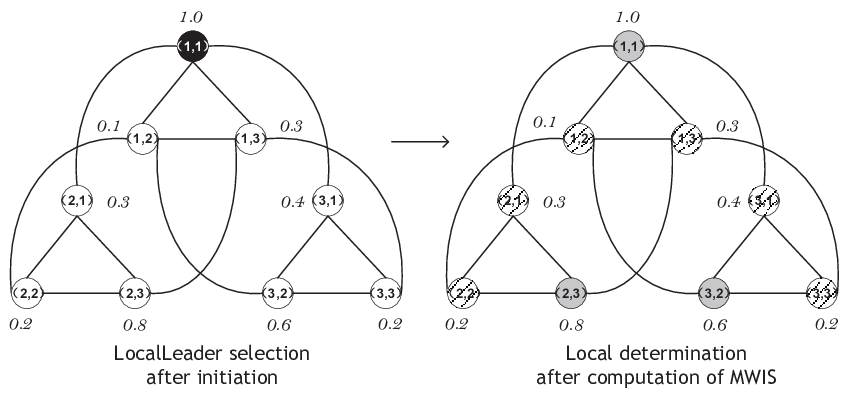
Herein we first present the achieved approximation ratio after mini-rounds. The results on mini-rounds will be presented in later analysis.
Theorem 3
Algorithm 3 achieves the same approximation ratio as the centralized robust PTAS in .
Proof:
Let be a LocalLeader selected at mini-round . In each mini-round, a LocalLeader utilizes the robust PTAS to find in its effective -hop neighborhood. Thus, each computed by a LocalLeader is -approximation to . Let be the global optimum, and be intersection of and , we have . As union of in all mini-rounds is exactly and any two distinct do not intersect, we have the union of all output by all LocalLeaders is -approximation to the global optimum in weight. ∎
Complexity.
We summarize complexity in a complete round.
Communication complexity: As shown in Fig. 2,
local broadcast happens times in each round,
respectively for WB, LD, and LB.
WB could be finished within mini-timeslots ,
which costs each vertex number of messages in worst case.
LD is done by a LocalLeader in its -hop neighborhood, then it costs mini-timeslots,
and each vertex passing messages.
In LB, each LocalLeader has to broadcast the results within its -hop neighborhood.
There are at most number of LocalLeaders
within any -hop neighborhood of any vertex.
Thus it costs mini-timeslots , and communication complexity .
Totally, it requires mini-timeslots , and each vertex number of passing messages .
Computation complexity:
The main computation cost is caused by LMWIS, as LS can be finished instantly.
In every mini-round, we use complete enumeration to compute local MWIS in each .
Suppose there are nodes in corresponding -hop neighborhood of , then .
Since , there are totally enumerations.
Using , we have
| (12) |
Hence, it requires polynomial time per mini-round,
and per round.
In practice, we can use more efficient constant approximation algorithm instead,
the communication complexity reduces to with a worse approximation ratio.
Space complexity:
It is , as each vertex has to store weight of neighbors within -hop neighborhood.
In our protocol, and is constant, then the communication, computation, and space complexity is , , and respectively.
IV-D Improve to constant-time-complexity strategy decision
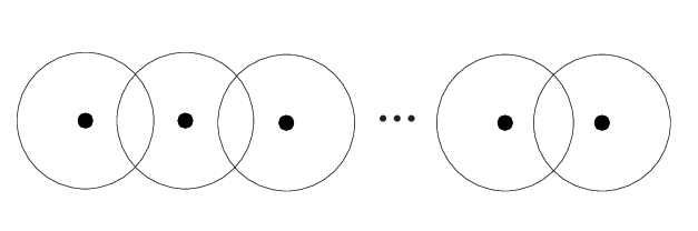
As mentioned previously, the distributed implementation of strategy decision requires mini-rounds to get all vertexes marked. We then show a simple instance of the worst case in Fig. 5. In the figure we use a linear network where all vertexes are aligned uniformly along a line within -hop distance. One can easily figure out that when the weight of each vertex is in a decreasing order from the start vertex to the end vertex, at the beginning only the start vertex can be LocalLeader since no other vertexes are locally maximum weighted. And, in each next round, still only one could be LocalLeader sequently. Thus it would take mini-rounds in a single round.
We then analyze the time complexity under random networks where location of each vertex is uniformly random distributed. We assume a random network has an average degree of . We expect to show it is possible to achieve a slightly smaller constant-approximation ratio if the algorithm terminates after a fixed number of mini-rounds, no matter whether there remains vertexes unmarked or not. Surprisingly, we find that it is indeed the case. The following theorem presents our results.
Theorem 4
Given a random network with an average degree , Algorithm 3 achieves -approximation to the optimum if we set the number of mini-rounds as a constant . is a constant with constant probability.
IV-E Practical regret
Now we analyze practical regret (or effective throughput) that considers the missed throughput due to time spent on learning. Let and respectively be length of a single round and mini-round. Time for strategy decision and data transmission denoted by and . In the strategy decision, supposing it requires mini-rounds, one for weight update, others for strategy decision, then . The actual data rate gained at each round is , where . The actual distance between and a strategy is . Thus in a round, the more time for learning, the larger regret it will be. In practice, we cannot use very long round as shall be smaller than channel coherence time.
Using as the approximation ratio, and as the maximum distance between the actual mean throughput of and , we obtain the practical regret is less than according to [14], i.e.,
Theorem 5
The practical regret of Algorithm 2 satisfies
| (13) | |||||
Then our channel allocation scheme can guarantee an effective throughput of .
V Simulations
Now we conduct simulations for our proposed channel accessing scheme under random networks. We set three series of simulations to respectively study efficiency, regret and influence of stale weight. In all simulations we run Algorithm 3 with . We set types of channels with data rates (units kbps) 150, 225, 300, 450, 600, 900, 1200, and 1350 respectively [12]. Each channel evolves as a distinct i.i.d Gaussian stochastic process over time. We set each round has length of a unit time slot. Referring to a cognitive radio system [12], we list the values of time parameters of a round in Table II. In strategy decision of each round, we set . Let be time to finish local broadcast and be the total time for local computation (LocalLeader selection and local MWIS computation). We have . According to Fig. 2, the actual throughput gained at each round is in our setting.
| round | ms | local broadcast | ms |
| local computation | ms | data transmission | ms |
V-A Efficiency of Algorithm 3
We first set a series of experiments to show efficiency of Algorithm 3. We plot the summed weight of all output MWISs by mini-round to for various random networks. The value of is respectively set as , , , , , and . From the Fig. 6, we can see that every line converges to a fixed value after the th mini-round, no matter how many vertexes there are in the extended graphs. This indicates that all vertexes are marked by that time. The results coincide with Theorem 4 where we claim that our proposed algorithm converges to a constant approximation ratio that is almost optimal under random graphs.

V-B Regret analysis
In the second series of experiments, we study practical regret and -regret caused by our proposed distributed learning scheme. We compare our method with LLR learning policy [11]. According to definition of regret and -regret, we need to compute the optimal throughput gained by the static best channel allocation. As the MWIS problem is NP-hard to solve, we construct a small network where we could find the optimum by brute force easily. Here we randomly generate a connected network with users, each having channels available. Using mean date rate of each channel as weight, we obtain the weight of the resulting MWIS or optimal throughput of the network, i.e., .
We then compare the optimal throughput, of the optimal throughput, with the effective throughput gained by the two learning algorithms. The results are shown in Fig. 7, which plots changes of practical regret and -regret as time increases. In both figures, our proposed algorithm outperforms the LLR learning policy. However, the practical regret compared to the optimum is far beyond , which indicates a significant impact caused by the time on learning. The ideal regret without practical consideration will tend to as the effective throughput is only half of the observed throughput in our setting. As to practical -regret, recall that when the reward of selected strategy is greater than of the best reward, the corresponding regret is negative. Fig. 7 (b) also shows that the -regret converges to a negative value, indicating that the achieved throughput by both algorithms is much better than of the optimum, even considering missed throughput on learning.


V-C Throughput performance under unfrequent update
We evaluate the effective throughput under different frequencies of weight update in the third series of simulation, where meanwhile we compare performance of our learning policy with LLR policy. In our proposed algorithm, initially each vertex has to collect weight of neighbors inside -hop neighborhood. If weight as well as corresponding strategy decision is updated at every time slot, it will cause high communication and communication cost that significantly affects effective throughput of data transmission. Instead, we can update weight every period that consists of time slots. Then we just need to do strategy decision at the beginning, and repeat data transmission times. The length of a period is . The actual average throughput gained at the period is We conduct experiments in a random network with users and channels. For such a large scale network, we will not compute the best static strategy as it can not be finished instantly. Instead, we record the average observed throughput up to period , where and average estimated throughput (i.e., average estimated weight of all selected strategies throughput up to ). Let be average estimated throughput at period, we have and The difference between and can also indicate the throughput performance of the algorithm.
We study the frequent case with , and unfrequent cases with stale weight that is updated periodically with time slots. We conduct each experiment respectively in time slots, each updating weight times. The actual effective throughput will be around of the ideal throughput without time consuming on strategy decision. In Fig.8, we can find that the average actual throughput achieved by both of the algorithms grows to the ideal throughput as a period lasts more time slots. Especially, a significant improvement can be seen between the frequent case (Fig.8(a)) and the unfrequent case of (Fig.8(b)). In the later two cases, further improvement is not so obvious as the proportion of time on learning decreases much more slowly. We then compare performance of the two learning policies. In each case, we can find that our adopted learning policy is much more accurate than the LLR learning policy. The difference between the estimated average throughput and the actual throughput is quite small in our adopted learning policy, while it is large in the LLR policy. Except the line of estimated throughput by LLR, difference among other three lines is not obvious in the figures. Thus we show a zoom-in part of the difference on the upper right of each figure. In these figures, it shows that the actual throughput achieved by our learning policy is better the LLR policy. They collaboratively show that unfrequent update has negligible impact on accuracy of estimation, but significantly improve effective throughput.


VI Related works
There is a rich body of results on dynamic spectrum access in cognitive radio networks. As channel availability and quality is unknown to secondary users, they need to conduct a learning process to select good channels. Several literatures address this problem from sequential decision perspective by MAB approaches, and several from a game theoretic perspective by convergence of equilibrium.
The results using MAB start from single-user play [21][22], where each channel evolves as independent and identically distributed Markov process with good or bad state. The results are then extended to multi-user play where more than secondary users select channels among ones [1], [2], [3], [4], [5], [6], [7]. These works basically assume channel quality evolving with i.i.d stochastic process over time, and a single-hop network setting where conflict happens if any pair of users choose the same channel simultaneously. For instance, Shu and Krunz [23] propose a throughput-optimal decision strategy with stochastic homogeneous channels. This optimal strategy has a threshold structure that indicates whether the channel is good or bad. Anandkumar et al. [6] propose two distributed learning and allocation schemes respectively for the case of pre-allocated ranks for secondary users and non such prior information.
On the other hand, some results consider dynamic spectrum access from an adaptive, game theoretic learning perspective. M. Maskery, et al.[24] model the dynamic channel process as a non-cooperative game for stochastic homogeneous channels, and basically rely on CSMA mechanism to estimate probability of channel contention. In the case of heterogeneous channel quality, Xu et al. [25] construct a potential game to maximize the expected throughput of all secondary users. They implicitly assume a single-hop network case where all users have the same probability to access channels.
We also review the results on network capacity, and related link scheduling problem that maximizes the channel capacity. There are numerous literatures in this line of work[26], [27], [28], [29], originating from the milestone work by Tassiulas et al. [30]. Though both maximizing throughput, the main difference of capacity problems is that they study throughput performance under a known environment without uncertainty of channel quality. The concerned issue is that interference among links constrains the maximum supportable arrival rate at each link that is assumed to have unit capacity. While the problem considered in our work focuses on throughput maximization under unknown and changing link quality, as well as existence of interference. We need to minimize loss of throughput caused by learning, as well as time and communication complexity of learning and their impact on throughput performance.
VII Conclusion
We proposed an almost throughput optimal channel accessing scheme for multihop cognitive networks. Our scheme consists of a distributed learning process with low computation and space complexity, and a strategy decision process with low computation and communication complexity. Our distributed implementation does not need extra predefined information on network parameters.
Our works have assumed i.i.d stochastic gain of channels, which is an easy-to-analyze model. Future work will take consideration of adversary case where gains are generated by an adversary that may obliviously or adaptively learn to play against our strategies. Additionally, most works as well as ours minimize weak regret compared to the best static policy, it will be challenging to computation-efficiently minimize strong regret compared to the best dynamic policy.
References
- [1] K. Liu and Q. Zhao, “Distributed learning in multi-armed bandit with multiple players,” IEEE Transactions on Signal Processing, vol. 58, no. 11, pp. 5667–5681, 2010.
- [2] C. Tekin and M. Liu, “Online learning in decentralized multiuser resource sharing problems,” arXiv preprint arXiv:1210.5544, 2012.
- [3] D. Kalathil, N. Nayyar, and R. Jain, “Decentralized learning for multi-player multi-armed bandits,” in Proc. of IEEE CDC, 2012, pp. 3960–3965.
- [4] H. Liu, K. Liu, and Q. Zhao, “Learning in a changing world: Restless multiarmed bandit with unknown dynamics,” IEEE Transactions on Information Theory, vol. 59, no. 3, pp. 1902–1916, 2013.
- [5] A. Anandkumar, N. Michael, and A. Tang, “Opportunistic spectrum access with multiple users: learning under competition,” in Proc. of IEEE INFOCOM, 2010, pp. 1–9.
- [6] A. Anandkumar, N. Michael, A. K. Tang, and A. Swami, “Distributed algorithms for learning and cognitive medium access with logarithmic regret,” IEEE Journal on Selected Areas in Communications, vol. 29, no. 4, pp. 731–745, 2011.
- [7] Y. Gai and B. Krishnamachari, “Decentralized online learning algorithms for opportunistic spectrum access,” in Proc. of IEEE GLOBECOM, 2011, pp. 1–6.
- [8] T. L. Lai and H. Robbins, “Asymptotically efficient adaptive allocation rules,” Advances in applied mathematics, vol. 6, no. 1, pp. 4–22, 1985.
- [9] P. Auer, N. Cesa-Bianchi, and P. Fischer, “Finite-time analysis of the multiarmed bandit problem,” Machine learning, vol. 47, no. 2-3, pp. 235–256, 2002.
- [10] R. Agrawal, “Sample mean based index policies with O (log n) regret for the multi-armed bandit problem,” Advances in Applied Probability, pp. 1054–1078, 1995.
- [11] Y. Gai, B. Krishnamachari, and R. Jain, “Combinatorial network optimization with unknown variables: Multi-armed bandits with linear rewards and individual observations,” IEEE/ACM Transactions on Networking, vol. 20, no. 5, pp. 1466–1478, 2012.
- [12] X.-Y. Li, P. Yang, Y. Yan, L. You, S. Tang, and Q. Huang, “Almost optimal accessing of nonstochastic channels in cognitive radio networks,” in Proc. of IEEE INFOCOM, 2012, pp. 2291–2299.
- [13] T. Nieberg, J. Hurink, and W. Kern, “A robust ptas for maximum weight independent sets in unit disk graphs,” Graph-theoretic concepts in computer science, pp. 214–221, 2005.
- [14] Y. Zhou and X.-Y. Li, “Multi-armed bandits with combinatorial strategies under stochastic bandits,” arXiv preprint: http://arxiv.org/abs/1307.5438, 2013.
- [15] T. Erlebach, K. Jansen, and E. Seidel, “Polynomial-time approximation schemes for geometric intersection graphs,” SIAM J. Comput., vol. 34, no. 6, pp. 1302–1323, Jun. 2005.
- [16] F. Kammer, T. Tholey, and H. Voepel, “Approximation algorithms for intersection graphs,” pp. 260–273, 2010.
- [17] F. Kuhn, T. Moscibroda, T. Nieberg, and R. Wattenhofer, “Fast deterministic distributed maximal independent set computation on growth-bounded graphs,” in Distributed Computing. Springer, 2005, pp. 273–287.
- [18] S.-H. Huang, P.-J. Wan, J. Deng, and Y. S. Han, “Broadcast scheduling in interference environment,” IEEE Transactions on Mobile Computing , vol. 7, no. 11, pp. 1338–1348, 2008.
- [19] Y. Wang, W. Wang, and X.-Y. Li, “Distributed low-cost backbone formation for wireless ad hoc networks,” in Proc. of ACM MOBIHOC, 2005, pp. 25–27.
- [20] F. Zou, Y. Wang, X.-H. Xu, X. Li, H. Du, P. Wan, and W. Wu, “New approximations for minimum-weighted dominating sets and minimum-weighted connected dominating sets on unit disk graphs,” Theoretical Computer Science, vol. 412, no. 3, pp. 198–208, 2011.
- [21] Q. Zhao, B. Krishnamachari, and K. Liu, “On myopic sensing for multi-channel opportunistic access: Structure, optimality, and performance,” IEEE Transactions on Wireless Communications, vol. 7, no. 12, pp. 5431–5440, 2008.
- [22] S. Ahmad, M. Liu, T. Javidi, Q. Zhao, and B. Krishnamachari, “Optimality of myopic sensing in multichannel opportunistic access,” IEEE Transactions on Information Theory, vol. 55, no. 9, pp. 4040–4050, 2009.
- [23] T. Shu and M. Krunz, “Throughput-efficient sequential channel sensing and probing in cognitive radio networks under sensing errors,” in Proc. of ACM MOBICOM, 2009, pp. 37–48.
- [24] M. Maskery, V. Krishnamurthy, and Q. Zhao, “Decentralized dynamic spectrum access for cognitive radios: cooperative design of a non-cooperative game,” IEEE Transactions on Communications, vol. 57, no. 2, pp. 459–469, 2009.
- [25] Y. Xu, J. Wang, Q. Wu, A. Anpalagan, and Y.-D. Yao, “Opportunistic spectrum access in unknown dynamic environment: A game-theoretic stochastic learning solution,” IEEE Transactions on Wireless Communications, vol. 11, no. 4, pp. 1380–1391, 2012.
- [26] C. Joo, X. Lin, and N. B. Shroff, “Understanding the capacity region of the greedy maximal scheduling algorithm in multi-hop wireless networks,” in Proc. IEEE INFOCOM, 2008, pp. 1103–1111.
- [27] M. Kodialam and T. Nandagopal, “Characterizing the capacity region in multi-radio multi-channel wireless mesh networks,” in Proc. of MOBICOM, 2005, pp. 73–87.
- [28] L. Jiang and J. Walrand, “A distributed CSMA algorithm for throughput and utility maximization in wireless networks,” IEEE/ACM Transactions on Networking, vol. 18, no. 3, pp. 960–972, 2010.
- [29] S.-J. Tang, X.-Y. Li, X. Wu, Y. Wu, X. Mao, P. Xu, and G. Chen, “Low complexity stable link scheduling for maximizing throughput in wireless networks,” in Proc. of IEEE SECON, 2009, pp. 1–9.
- [30] L. Tassiulas and A. Ephremides, “Stability properties of constrained queueing systems and scheduling policies for maximum throughput in multihop radio networks,” IEEE/ACM Transactions on Automatic Control, vol. , pp. 1936–1948, 1992.