A Precision Measurement of Charm Dimuon Production in Neutrino Interactions from the NOMAD Experiment
Abstract
We present our new measurement of the cross-section for charm dimuon production in neutrino-iron interactions based upon the full statistics collected by the NOMAD experiment. After background subtraction we observe 15,344 charm dimuon events, providing the largest sample currently available. The analysis exploits the large inclusive charged current sample - about events after all analysis cuts - and the high resolution NOMAD detector to constrain the total systematic uncertainty on the ratio of charm dimuon to inclusive Charged Current (CC) cross-sections to . We also perform a fit to the NOMAD data to extract the charm production parameters and the strange quark sea content of the nucleon within the NLO QCD approximation. We obtain a value of GeV/c2 for the running mass of the charm quark in the scheme and a strange quark sea suppression factor of at GeV2/c2.
Keywords:
Charm production, strange quark content of the nucleon, dimuon charm production, neutrino interactionsPACS
13.15.+g , 13.85.Lg , 14.60.Lm1 Introduction
The process of charm dimuon production stems from the charged-current (CC) production of a charm quark, which semileptonically decays into a final state secondary muon with its electric charge opposite to that of the muon from the leptonic CC vertex. Figure 1 shows a schematic Feynman diagram of the process. The Deep Inelastic Scattering (DIS) production of charm quarks involves the scattering off both the strange and the non-strange quark content of the nucleon. However, the contributions from - and -quarks are suppressed by the small quark-mixing Cabibbo-Kobayashi-Maskawa (CKM) matrix elements.
A measurement of the cross-section for charm dimuon production in neutrino DIS off nucleons provides the most direct and clean probe of , the strange quark sea content of the nucleon. Inclusive cross sections are indeed not very sensitive to the strange quark sea content, since, in this case, the complementary contributions from strange and non-strange distributions are strongly anti-correlated. In addition, the flavor selection offered by neutrino and anti-neutrino interactions allows a determination of both and separately. The strange quark contribution is particularly important at small values of the parton momentum fractions , where the quark distributions are dominated by the sea. This kinematic region is crucial in high-energy hadron collisions for the study of many processes and therefore an accurate determination of the strange sea is required for the interpretation of experimental data. The knowledge of the strange quark sea content of the nucleon and of charm production is also the dominant contribution to the systematic uncertainties in the electroweak measurements from (anti)neutrino DIS interactions [1].

Traditionally, charm dimuon production in (anti)neutrino interactions has always been measured in massive calorimeters, mainly composed of passive heavy materials (iron, marble, lead etc.) in order to obtain a sizeable number of events [2, 3, 4, 5, 6, 7, 8]. This detection technique, while relatively simple and efficient, is ultimately limited by the coarse resolution of the detectors and by the resulting systematic uncertainties.
The high resolution NOMAD data allow a new level of precision in the measurement of charm dimuon production in neutrino interactions. The use of a low density target located inside a magnetic spectrometer measures the momentum and emission angle of all secondary particles produced in neutrino interactions. Additionally, the detector offers the capability of making redundant in situ measurements of all relevant backgrounds, minimizing the reliance on Monte Carlo simulation (MC) of the hadronization process. For the first time a high resolution reconstruction of neutrino interactions can be achieved from high statistics samples, typical of the most massive calorimeters but without the corresponding limitations. Furthermore, the neutrino spectrum in NOMAD is well suited to study charm production close to the charm threshold, providing enhanced sensitivity to the charm production parameters.
This paper is organized as follows. Section 2 gives a short overview of the charm dimuon production in neutrino charged current interactions. In Section 3 we describe the neutrino beam and the NOMAD detector used for our measurement. Section 4 explains our event selection and the corresponding cuts. In Section 5 and Section 6 we describe the analysis scheme used for our precision measurement and the unfolding procedure needed to extract the final cross-sections, respectively. We present our final NOMAD results in Section 7 and provide a detailed discussion of systematic uncertainties in Section 8. Section 9 discusses the extraction of charm production parameters and of the strange quark sea content of the nucleon from NOMAD data. Finally, Section 10 gives a summary of the main results achieved.
2 Charm dimuon production in neutrino interactions
The differential cross section for charm quark production in CC neutrino DIS off nucleon or nuclear target can be written as:
| (1) |
where , , and are common DIS variables, is the neutrino energy, is the Fermi constant, and are the nucleon and -boson masses, respectively, and are the corresponding structure functions (SFs). For an isoscalar target, assuming the usual isospin relations between the proton and neutron quark distributions, we have in the LO QCD approximation 11 1 We give the Leading Order (LO) approximation for illustration purpose only. The entire analysis described in this paper is performed in the Next to Leading Order (NLO) or Next to Next to Leading Order (NNLO) approximation, including both the cross-section calculation and the acceptance corrections.:
| (2) |
where are the light quark distributions in the proton, is the slow-rescaling variable appearing in the kinematics of parton scattering with one massive particle in the final state [10], and is the charm quark mass. The values of the CKM matrix elements and [11] suggest that the strange quark contribution dominates the cross section of Eq. (1) at small . In the NLO QCD approximation the structure functions of Eq. (2) get an additional contribution from the gluon-radiation and gluon-initiated processes [12].
Due to their larger mass, the sea strange quarks are suppressed with respect to the and sea quarks. The strange sea suppression factor:
| (3) |
increases with the momentum transfer .
Experimental data on neutrino induced DIS charm production is typically collected on heavy targets (e.g. iron), rather than on free nucleons. Nuclear corrections must then be applied to the structure functions entering the cross-section in order to take into account the effect of the nuclear medium. In general, nuclear corrections in neutrino interactions are different from those for charged-lepton interactions [13] and can be described to a good accuracy by the model of Ref.[13, 14, 15].
In the LO the dimuon cross section is related to the corresponding cross section for charmed-quark production as:
| (4) |
where is the production fraction of the charmed hadron , is the fragmentation function of the charm quark into a given charmed hadron carrying a fraction of the charm quark momentum, and is the corresponding inclusive branching ratio for the muon decays 22 2 The normalization is defined such that .. Here refers to a generic charmed baryon. At NLO the coefficient functions entering the SFs calculation depend, in general, on as well. The charm fragmentation function defines the energy of the outgoing charmed hadron and, in turn, of the secondary muon produced in the semileptonic decay. Assuming a universal for all charmed hadrons and integrating over , Eq. (4) becomes , where is the effective semileptonic branching ratio, and the universal fragmentation function can be described by the Collins-Spiller parameterization [16]:
| (5) |
with as a free parameter. This parameterization has a more accurate asymptotic behavior in the limit of than the Peterson form [41]. The charmed fractions depend on the incoming neutrino energy. This fact can be explained by the contributions from quasi-elastic and diffractive production. Measurements of and in neutrino interactions were performed by the E531 [17, 18] and CHORUS [19, 20] experiments using the emulsion detection technique, which allowed them to reconstruct exclusive final states.
3 Beam and Detector
The Neutrino Oscillation MAgnetic Detector (NOMAD) experiment at CERN used a neutrino beam produced by the 450 GeV protons from the Super Proton Synchrotron (SPS) incident on a beryllium target and producing secondary , , and mesons. The positively charged mesons were focussed by two magnetic horns into a 290 m long evacuated decay pipe. Decays of , , and produced the SPS neutrino beam. The average neutrino flight path to NOMAD was 628 m, the detector being 836 m downstream of the Be-target. The SPS beamline and the neutrino flux incident at NOMAD are described in [21]. The -flux in NOMAD can be estimated from the and production measurements in proton-Be collision by the SPY experiment [22, 23, 24] and by an earlier measurement conducted by Atherton et al. [25]. The -integrated relative composition of CC events, constrained in situ by the measurement of CC-interactions of each of the neutrino species, is . Thus, 97.5% of the events are induced by neutrinos with a small anti-neutrino contamination.
The NOMAD apparatus, described in [26], consisted of several sub-detectors. The active target comprised 132 planes of m2 drift chambers [27] (DCH) with an average density similar to that of liquid hydrogen (0.1 gm/cm3). On average, the equivalent material in the DCH encountered by particles produced in a -interaction was about half of a radiation length and a quarter of a hadronic interaction length (). The fiducial mass of the NOMAD DCH-target, 2.7 tons, was composed primarily of carbon (64%), oxygen (22%), nitrogen (6%), and hydrogen (5%) yielding an effective atomic number, A=12.8, similar to carbon. Downstream of the DCH, there were nine modules of transition radiation detectors [28] (TRD), followed by a preshower (PRS) and a lead-glass electromagnetic calorimeter [29] (ECAL). The ensemble of DCH, TRD, and PRS/ECAL was placed within a dipole magnet providing a 0.4 T magnetic field orthogonal to the neutrino beam line. Downstream of the magnet was a hadron calorimeter, followed by two muon stations each comprising large area drift chambers (MCH) and separated by an iron filter. The two stations, placed at 8- and 13-’s downstream of the ECAL, provided a clean identification of the muons. The charged tracks in the DCH were measured with an approximate momentum () resolution of ( in GeV/ and in meters) with unambiguous charge separation in the energy range of interest. The energy deposition from and were measured in ECAL with an energy resolution of ( in GeV). The experiment recorded over 1.7 million neutrino interactions in the active drift-chamber target in the range GeV.
The detector was suspended from iron pillars (the ‘I’s) at the two ends of the magnet. The front pillar was instrumented with scintillators to provide an additional massive active target for neutrino interactions, the front calorimeter (FCAL). The FCAL consisted of 23 iron plates 4.9 cm thick and separated by 1.8 cm gaps. Twenty out of the 22 gaps were instrumented with long scintillators, which were read out on both ends by 3 in photomultipliers. The dimensions of the scintillators were cm3. To achieve optimal light collection and a reasonable number of electronic channels five consecutive scintillators along the beam axis were ganged together by means of twisted light guides to form a module. Ten such modules were placed above each other to form a stack. Four stacks were placed along the beam axis. The area of the FCAL ”seen” by the neutrino beam was cm2. The detector had a depth of about five nuclear interaction lengths and a total fiducial mass of about 17.7 tons, composed mainly of iron. The energy deposition in FCAL was measured with a resolution ( in GeV). The experiment recorded over 18 million neutrino interactions in the FCAL in the range GeV.
In front of the FCAL there was a plane of scintillators, , used to veto charged particles entering the detector. Before and after the TRD there were two planes of scintillators, and , whose coincidence provided the main trigger for charged tracks in the drift chamber volume.
The schematic of the FCAL and the DCH-tracker with a charm dimuon event candidate is shown in Figure 2.

4 Event Selection
4.1 Trigger and Calibration
The main trigger selection used for the analysis of FCAL data requires an energy deposition in the FCAL of at least 3.15 m.i.p. - m.i.p. is the signal of a minimum ionizing particle crossing one FCAL stack - and no signal in the veto scintillator plane: - (FCAL trigger). This trigger vetoes through-going muons and has a live time of .
A second independent trigger selection with lower threshold is used to measure the FCAL trigger efficiency from data (FCAL′ trigger). For this trigger an energy deposition of at least 1.2 m.i.p. in the FCAL is requested, in addition to the coincidence with a signal from the scintillator plane in the TRD region: . The live time is .
We measure the efficiency of the FCAL trigger directly from data in the following way:
| (6) |
We determine the FCAL trigger efficiency separately for each of the 4 stacks and each of the 4 years of data taking, for a total of 16 configurations. The final trigger efficiency is obtained by averaging over the different stacks and years of data taking, weighted by the corresponding numbers of CC events identified in the data.
In order to take into account the saturation of the readout electronics, which resulted in a reduced value of the ADC counts observed in the data at high energies, we apply a correction function to the ADC response of each individual FCAL module in the Monte Carlo. This correction function is obtained by minimizing the between the total energy distributions in the FCAL for CC events in data and Monte Carlo.
The energy deposited in each stack, , is calculated as the sum of the energy depositions (in m.i.p.) of the ten individual FCAL modules (in m.i.p.)in the stack:
| (7) |
The relative calibration of individual modules in m.i.p. (ADC to m.i.p) is performed by using the energy deposition of high energy muons from SPS secondary beams crossing the FCAL in between neutrino spills. The muon tracks are reconstructed in the drift chambers and extrapolated back to the FCAL. The absolute energy deposition in GeV is then obtained by dividing the values of by the appropriate mip/GeV conversion factor :
| (8) |
The constant is obtained from the default MC simulation by comparing the reconstructed to the simulated energy and is validated by the analysis of single muon events in data.
After determining the response function between the simulated energy and the energy reconstructed in FCAL , we extract the inverse function from the MC simulation by comparing separately the simulated and reconstructed shower energy for events originated in each stack. The reconstructed shower energy is obtained by subtracting the energy loss by the muons from the total energy measured in FCAL.
4.2 Analysis cuts
The analysis of FCAL data proceeds with the selection of two independent samples: a) inclusive CC events with a single negatively charged muon; b) dimuon events. All the applied cuts are relatively loose in order to avoid potential biases of the samples and to retain a large signal efficiency. In addition, we try to use similar selection cuts (if applicable) for both the dimuon and the CC samples. These criteria minimize systematic uncertainties from the event selection procedure. We identify two different dimuon samples: the Opposite Sign Dimuons (OSDM) with two muons of opposite charge, and the Like Sign Dimuons (LSDM) with two muons of the same charge (background sample).
The momenta of the identified muons, for the primary muon and for the secondary one, are measured with high precision with the DCH located in the low density spectrometer following FCAL. We define the primary muon as the one with the largest transverse momentum relative to the beam direction. The total hadronic energy of the event, , is calculated from the sum of the energy of the hadronic shower measured in FCAL and the energy of the secondary muon and of any other charged track measured in the drift chambers, minus the energy loss of the primary and secondary muons in FCAL. The reconstructed neutrino energy is obtained as the sum of the energy of the primary muon and the total hadronic energy: . The DIS kinematic variables are reconstructed in the following way:
where is the angle of the primary muon with respect to the neutrino beam direction in the lab frame and is the mass of the proton.
The applied cuts are:
- 1
FCAL trigger and good run.
- 2
One negatively charged muon, , identified by the MCH.
- 3*
A second muon, , identified by the Muon System: either a from -quark production/background or a from background.
- 4
Fiducial volume inside one of the 4 FCAL stacks. The coordinates of the primary vertex, and , are determined from the extrapolation of the muon(s) to the middle point of the most upstream stack containing energy and are constrained to: cm and cm.
- 5*
Time difference between the two muons, as measured from the first hit in the drift chambers, less than 5ns to reject accidental backgrounds.
- 6*
Require a leading negative muon as the one with the largest transverse momentum relative to the beam direction, . This cut rejects the background from charm dimuon events originated by the small anti-neutrino contamination of the beam. We require the presence of only one negative muon in the event for the CC selection.
- 7*
Energy of the hadron shower without the energy of the muon from charm decay () less than GeV and GeV.
- 8
.
- 9
Energy of the primary muon more than GeV. We note that GeV is practically the minimal energy for muons to reach the MCH and be identified as muons in the NOMAD detector.
- 10
Energy of the secondary muon more than GeV or GeV for CC.
- 11
Four-momentum transfer GeVc2.
where the cuts marked with * refer mainly to the dimuon sample. The main goal of the selection is to ensure that the events are well measured in FCAL. We limit our analysis to the region GeVc2 in which we can realiably calculate the cross-sections within the parton model. It must be also noted that the impact of the cut on the charm sample is negligible, due to the intrinsic production threshold. Tables 1 summarizes the effect of the CC selection. A subsample () of the data analyzed for this paper was the subject of an earlier NOMAD publication [4].
We normalize the number of CC events in the MC to the ones observed in the data after the fiducial volume and leading muon cuts (cut 6 in Table 1). The number of charm dimuon events in MC is normalized to the number of inclusive CC events multiplied by the cross-section ratio in our model.
| MC | DATA | DATA/MC | ||
|---|---|---|---|---|
| Cut | Rec. | Eff. | Rec. | |
| (Trig.) | 12143746 | — | 12401729 | 1.021 |
| () | 12126348 | — | 12298205 | 1.014 |
| (FV) | 10639388 | 76.1% | 10757864 | 1.011 |
| (Lead. ) | 10636157 | 76.1% | 10636157 | 1.000 |
| () | 10582711 | 75.7% | 10576596 | 0.999 |
| () | 10359121 | 74.1% | 10381255 | 1.002 |
| () | 10354170 | 74.1% | 10376815 | 1.002 |
| () | 9730058 | 69.6% | 9615738 | 0.988 |
| () | 9175383 | 65.8% | 8759065 | 0.954 |
5 Analysis scheme
The analysis measures the ratio of the charm dimuon cross-section to the inclusive CC cross-section, as a function of the kinematic variables:
| (9) |
where and the partonic center of mass energy squared is defined as . The ratio provides a large cancellation of all systematic uncertainties affecting both the numerator and the denominator.
The CC events in the data are well reconstructed and have a negligible background. Figure 3 shows good agreement between data and Monte Carlo for the reconstructed kinematic variables in CC events.


The charm dimuon events are determined from the opposite sign dimuons measured in the data after subtracting the background:
| (10) |
The background to the opposite sign dimuon process arises from muonic decays of hadrons - primarily and mesons - produced in the hadronic shower or by hadrons which punch through to the MCH, thereby being misidentified as muons. The background from charm dimuon events originating by the interaction of the small anti-neutrino contamination of the beam is suppressed by the requirement of a leading muon with negative charge (cut 7). This selection cut correctly identifies the leading muon in about 95% of the events (Table 2). Since represent only about 5% of the flux, the final background from anti-neutrino charm dimuons will be at the level of . Similarly, other background sources like trident production, the overlap of a neutrino and an anti-neutrino event, or the production and subsequent muonic decay of in Neutral Current interactions are found to be negligible.
The background events are estimated from the LSDM events, measured in the data, in which both muons have the same negative charge, (), multiplied by a scale factor extracted from the MC:
| (11) |
where the scale factor is given by the ratio of opposite sign to like sign dimuon events originated from background events.


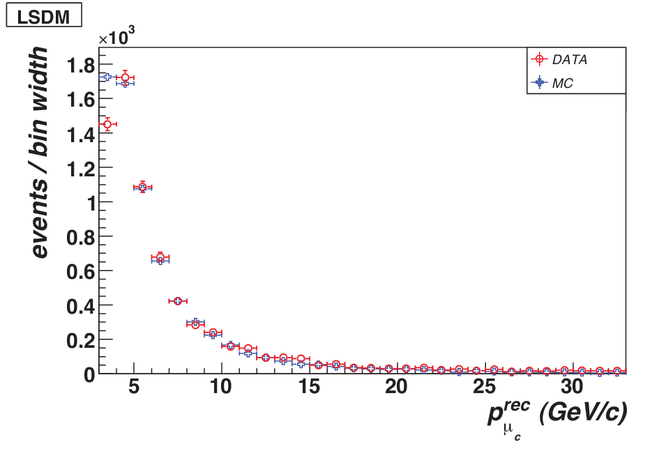
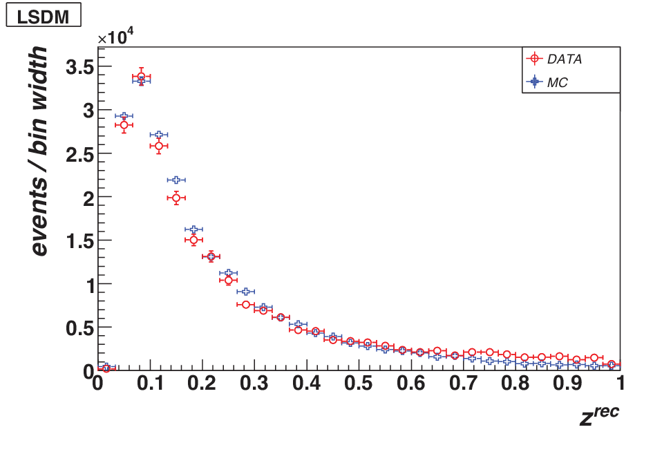
In order to reduce the MC statistical uncertainties we generated a total of about CC events fully reconstructed in FCAL. Figure 4 shows the distributions of the LSDM events in FCAL data and MC. The general agreement is adequate since LSDM events from MC are never directly used in our analysis. Rather, we only use the ratio of OSDM to LSDM background events in MC. This ratio is very sensitive to the details of the fragmentation of the hadronic system, in particular at low momenta. For this reason we cannot rely on the Monte Carlo simulation at the level of precision of a few percent. Instead, since the background scale is determined by the ratio of positively charged to negatively charged mesons inside the hadronic system produced by the fragmentation of partons in DIS events, we measure this ratio as a function of the meson momentum from the NOMAD data originated in the light Drift Chamber target (DCH). The differences of the inclusive fragmentation variable distributions between target nuclei (carbon in DCH vs. iron in FCAL) are found to be negligible based on a direct comparison between the corresponding MC samples. This comparison is shown in the top plot of Figure 5.

We exclude charged tracks which are either identified as electrons/positrons by the TRD or have a range consistent with protons. We then subtract the small residual proton/electron/positron contamination by using the MC. These contaminations are small even before rejecting identified tracks. The average ratio in neutrino interactions is only about 7% and therefore the uncertainty introduced in the measurement by the different and lifetimes is negligible. After measuring the ratio of positively charged to negatively charged mesons from DCH data, we re-weight each positive meson originated from the hadronic system in FCAL events according to the measured ratio :
| (12) |
As a result, the entire background estimate for the charm dimuon sample is based upon the data themselves, which are used both for the LSDM and for the background scale. We emphasize that only the use of a low density target embedded inside a magnetic spectrometer in NOMAD has allowed the use of this procedure. Figure 5 shows the measured ratio from the DCH data, as well as a comparison with the corresponding MC simulation and the function . The calibration of the background through the re-weighting procedure is a crucial step in the analysis and allows a substantial improvement in the description of the charm dimuon data by the Monte Carlo simulation. Without the use of data from the low density DCH target it would have not been possible to lower the energy threshold on the secondary muon down to 3 GeV as well as to reduce the systematic uncertainty on the background subtraction. Figure 6 shows the background scale as a function of the main kinematic variables with the re-weighting procedure according to Eq. (12). Table 2 summarizes signal and background events after each selection cut. After all cuts we retain 20,479 OSDM events in the data, of which 15,344 are genuine charm signal (75%) and 5,135 are background (25%). The final distributions of various kinematic variables for the charm data after background subtraction are given in Figure 7.
| MC | DATA | DATA/MC | |||||
|---|---|---|---|---|---|---|---|
| Cut | Rec. | Eff. | OSDM | LSDM | Bg. | Charm | |
| (FV) | 18783 | 27.0% | 30955 | 33127 | — | — | — |
| (Time) | 18671 | 26.9% | 26739 | 9488 | 6565 | 20174 | 1.080 |
| (Lead. ) | 18144 | 26.1% | 24642 | 9488 | 6366 | 18276 | 1.007 |
| () | 16287 | 23.4% | 21637 | 7763 | 5403 | 16234 | 0.997 |
| () | 16180 | 23.0% | 21256 | 7524 | 5308 | 15948 | 0.985 |
| () | 16173 | 23.0% | 21245 | 7518 | 5307 | 15938 | 0.985 |
| () | 16019 | 22.8% | 20949 | 7324 | 5269 | 15680 | 0.978 |
| () | 15684 | 22.5% | 20479 | 7148 | 5135 | 15344 | 0.978 |


Table 3 shows a comparison of our final charm dimuon sample with the previous measurements. The new NOMAD measurement has the highest available statistics of neutrino induced charm dimuon events. In particular, the measurement described in this paper has about 3 times the statistics of NuTeV and CCFR, which till now have been the only source of information on strange sea quark distributions in global Parton Distribution Function (PDF) fits [31]. Furthermore, the NOMAD sample can reach the lowest energy threshold, giving additional sensitivity to the charm production parameters.
| Exp. | Publ. | Stat. () | (GeV) | |
| CDHS [2] | 1982 | 8,600 | 30-250 (20) | |
| CHARM II [3] | 1999 | 3,100 | 35-290 (24) | |
| NOMAD [4] | 2000 | 2,714 | 14-300 (27) | |
| CCFR [5, 6] | 2001 | 5,030 | 30-600 (150) | |
| NuTeV [6, 7] | 2001 | 5,102 | 20-400 (157.8) | |
| CHORUS [8] | 2008 | 8,910 | 15-240 (27) | |
| NOMAD | 2013 | 15,344 | 6-300 (27) | |
| CDHS [2] | 1982 | 2,000 | 30-250 | |
| CHARM II [3] | 1999 | 700 | 35-290 | |
| CCFR [5, 6] | 2001 | 1,060 | 30-600 | |
| NuTeV [6, 7] | 2001 | 1,458 | 20-400 | |
| CHORUS [8] | 2008 | 430 | 10-240 |
6 Unfolding procedure
The detector smearing and acceptance corrections require an input model for the cross-sections and fragmentation functions. For the inclusive CC sample the model is largely independent from the NOMAD data. However, for the charm sample the NOMAD dimuon data are eventually used to determine the charm production parameters, which, themselves, are inputs to the experimental acceptance corrections. In our analysis we follow an iterative procedure. First, we use an input model which is fully independent from NOMAD data and we verify its consistency with the NOMAD data. After this step we add NOMAD data to the global PDF fits to improve the precision on the charm production parameters. We then feed back the modified model into the acceptance calculation and iterate until convergence. In the following sections we describe in details the model used and the corrections applied.
6.1 Cross-section weights
Neutrino interactions are simulated using a modified version of LEPTO 6.1 [32] and JETSET 7.4 [33] with and cutoff parameters removed. Final state interactions within the target nucleus are described by DPMJET [34]. A full detector simulation based on GEANT 3.21 [35] is then performed. The default DIS cross-sections are calculated in the LO approximation with the parton density functions from the GRV-HO parameterizations [36] available in PDFLIB [37]. This simulation does not adequately describe the charm production process since it does not include any rescaling mechanism to take into account the large mass of the charm quark. Furthermore, no electroweak, nuclear and High Twist corrections are included.
In order to achieve an accurate description of data, we implement a re-weighting procedure for the charm cross-section:
| (13) |
where is the original LEPTO cross-section used to generate the MC events and is the new cross-section obtained from an analytical calculation [13, 14, 15, 31, 38, 39]. The charm cross-section is calculated in the NLO QCD approximation for the heavy quark structure functions, in a factorization scheme with three light flavors in the initial state (FFS) [31]. The Target Mass Corrections (TMC) are implemented following the prescription by Georgi and Politzer [40]. The impact of the dynamical High Twist corrections to the charm production is evaluated by applying a simple rescaling for the quark charge to the phenomenological twist-4 terms extracted from the inclusive lepton-nucleon cross-sections [38]. We apply nuclear corrections using the calculations of Refs. [13, 14, 15]. This calculation takes into account a number of different effects including the nucleon Fermi motion and binding, neutron excess, nuclear shadowing, nuclear pion excess and the off-shell correction to bound nucleon Structure Functions (SF). The electroweak corrections, including one-loop terms, are calculated according to Ref. [39] within the framework of the parton model. The parameters related to charm production like the mass of the charm quark and the strange quark sea distribution are fixed to the ones extracted from the global PDF fit including NuTeV and CCFR charm dimuon data [31] at this stage. This allows a consistency check with a calculation fully independent from NOMAD data.
We extract the LEPTO cross-section from the NOMAD MC by simulating events with an input flux which is chosen to be inversely proportional to the neutrino energy .We then bin the events in the space and smooth the corresponding histograms with an interpolation procedure.
Finally, we apply an additional re-weighting to the charm events to take into account the effect of the charm fragmentation, which is described by the Collins-Spiller parameterization [16] (see Eq. (5)). This function describes the probability for a charmed hadron to carry a given fraction of the charmed quark logitudinal momentum and is defined by one free parameter . Figure 7 shows a comparison between data and weighted MC for different kinematic variables in charm dimuon events.
We apply a similar re-weighting procedure to the inclusive CC events (single muons). The model used for the inclusive CC structure functions on iron is the same described above for charm production. The light quark contributions to the SFs are calculated in the NNLO QCD approximation. Figure 3 shows a comparison between data and weighted MC for different kinematic variables in CC events.
6.2 Binning and hadronic energy correction
The binning of the data is performed in such a way that the size of each bin is comparable to the experimental resolution within that given bin. This procedure allows a reduction of correlations among different bins, thus minimizing systematic uncertainties. Overall we have 19 bins for , 14 bins for and 15 bins for .
After defining the binning we perform a calibration of the global hadronic energy scale. This procedure corrects for potential discrepancies between data and MC related to the simulation of neutral and charged particles in the hadronic jet orginated by the neutrino-nucleus interactions. We perform the calibration of the hadronic energy scale by using the distribution in inclusive CC events (single muon events). For each of the 19 bins in the reconstructed visible energy , we multiply the hadronic energy in MC events by a free scale factor , and we determine the optimal value of by minimizing the calculated from the distribution in data and MC. This technique relies upon the precise measurement of in the drift chambers (see Section 8.2). The best fit values for range from -0.1% to -3.7%, depending upon the bin considered. Finally we interpolate the corrections for each bin with a spline function in order to have a smooth behavior of the hadronic energy scale as a function of the visible energy which can be extrapolated to different binning definitions. The use of a separate calibration factor for each bin effectively takes into account differences in the development of the hadronic shower as a function of the neutrino energy (e.g. missing particles, fragmentation etc.). In general, we observe that the hadronic energy correction increases with the neutrino energy. As can be seen from Figure 8 the calibration of the global hadronic energy improves the agreement between data and MC for the distribution.
In order to estimate the corresponding uncertainties on we inflate the MC errors until the values of /dof at the minimum is equal to unity for each bin. We then calculate the error band as the range in which is resulting in . The uncertainties obtained for all bins range from 0.3% at low energy to about 1% at high energy.


6.3 Smearing matrix and efficiency correction
After re-weighting the MC events to our cross-section model, we unfold the detector response from the measured data for both the inclusive CC and the charm dimuon events. To this end we first determine the smearing matrix and the efficiency corrections from the MC simulation:
| (14) |
where and are the reconstructed and simulated variable (). The inverse of the above relation provides the unfolded measurement:
| (15) |
The impact of non-diagonal terms in the smearing matrix is reduced because the bin size is comparable to the experimental resolution.
We validate the unfolding procedure by splitting the available MC events in two independent samples. The first sample (biased) is used to extract the smearing matrix and the efficiency correction. The second half of the MC sample (unbiased) is used as fake data to determine the unfolded distributions. These latter are then compared with the input simulated variables of the unbiased sample. Our results indicate that we can reproduce the input distributions in the unbiased sample with a good accuracy for both CC and charm dimuon events. Finally we compare the unfolded distributions obtained from FCAL data and MC with an analytical calculation performed by convoluting our cross-section model with the neutrino flux.
6.4 Bin centering correction
The definition of the bin size is based on the procedure described in Section 6.2 for the reconstructed variables. The boundaries of the corresponding bins in the simulated variables are then slightly adjusted in order to keep the same statistical uncertainty as in the reconstructed variables.
Since the functions vary inside the chosen bins, we need to apply a bin centering correction to the unfolded data. To this purpose we use our model calculation convoluted with the NOMAD flux. For each bin, we find the value of the kinematic variable on the horizontal axis ( or ) for which the analytical function is equal to the corresponding average value inside the bin. We then assign the measured value of for the bin considered to this calculated point on the horizontal axis.
7 Results
7.1 Charm fragmentation
The measured kinematic distributions for charm events are sensitive to the charm fragmentation function, which gives the probability for the charmed hadron to carry a given fraction of the longitudinal momentum of the hadronic system. We model the charm fragmentation function with the Collins-Spiller parameterization [16] shown in Eq. (5), which has a more accurate asymptotic behavior in the limit of than the Peterson form [41]. The charm fragmentation function is folded with the NLO charm cross-section [31] through the re-weighting procedure implemented for all our MC events. This procedure allows a variation of the free parameter in the Collins-Spiller fragmentation function, together with the charm production parameters in the charm cross-section.
We use two kinematic distributions to detemine from our data: the energy of the secondary muon from charm decay, , and the scaling variable . The first one gives the most sensitive variable to fragmentation and has the advantage that it is largely independent from the details of the development of the hadronic shower inside FCAL, since the muon momentum is precisely measured in the drift chambers. Some additional sensitivity can be obtained from , while the remaining kinematic variables do not add any substantial contribution. We perform a simultaneous fit to both and by varying on an event-by-event basis in our MC re-weighting. The results are shown in Table 4. The correlation with the mass of the charm quark and with the strange sea parameterization turns out to be small in our fit since we mostly rely on the energy of the secondary muon to extract . A two-dimensional fit to and with both and as free parameters results indeed in a surface which is flat as a function of .
| Experiment | NOMAD (, ) | E531 () | NOMAD + E531 |
|---|---|---|---|
In order to reduce the uncertainty in the determination of , we also consider the direct measurement of charm production performed in nuclear emulsions by the E531 [42] experiment, which had an average neutrino energy comparable to NOMAD. This latter condition is crucial for our analysis, since the distribution of the measured fragmentation variable is expected to become softer by increasing the center of mass energy, due to gluon radiation. We re-fit the distribution of the charmed mesons 33 3 In nuclear emulsions the fragmentation variable is defined as the ratio between the energy of the primary charmed hadron and the energy trasfer . This variable is different from the measured in NOMAD, which is the ratio between the energy of the secondary muon originated in the semileptonic decay of the charmed hadrons and the energy transfer . published by E531 with the Collins-Spiller function. The value of that we obtain from E531 data is shown in Table 4 and is in good agreement with the value from the NOMAD analysis. We then use both the NOMAD and E531 data in a combined fit and obtain:
| (16) |
where the first uncertainty is due to statistics and the second one to systematics (see Section 8). This is our final result, which will be used in the following analysis. It is interesting to note that this result is consistent with the expectation [16] where represents the size of the hadron in momentum space and is the charm quark mass (see Section 9).
For the sake of comparison with previous measurements, we also performed a fit to the combined NOMAD and E531 data sets with the Peterson parameterization [41] of the charm fragmentation function and obtained .
7.2 Charm semileptonic branching ratio
The effective charm semileptonic branching ratio is expected to increase with increasing neutrino energy because the charmed fractions are themselves neutrino energy dependent. This in turn is due to the lower branching ratio to muon of the and coupled with the fact that quasi-elastic and diffractive production make a more important contribution at low energies. Since NOMAD dimuon data extend down to GeV we need to take into account the energy dependence of in our analysis.
The only existing measurement of the charmed fractions as a function of the neutrino energy comes from a re-analysis [18] of the data from the E531 experiment [17, 42]. A new determination of as a function of the neutrino energy was obtained in Ref. [31] from the E531 emulsion data. We fit the data from Ref. [31] with the following smooth function:
| (17) |
which has two free parameters and . The values of the parameters obtained from a fit to E531 data are given in Table 5. Figure 9 shows the results of the fit together with the uncertainty band on obtained from a global energy independent fit to the NuTeV and CCFR charm dimuon data for GeV [31]. The E531 data are consistent with the constant value of extracted at high energy from NuTeV and CCFR data in the common energy range. In the following we use Eq. (17) to parameterize in our analysis. If we add the NOMAD dimuon data to the E531 data and extract the and parameters from the corresponding fit (described in Section 9) we substantially reduce the uncertainties on and , as can be seen from Table 5.
| Experiment | (GeV) | |
|---|---|---|
| E531 | ||
| E531+NOMAD |

7.3 Ratios
The final results for the measured ratio as a function of the kinematic variables and are shown in Figures 10-12. The curves represent our model calculation based upon the global PDF fit including only NuTeV and CCFR data [31]. Our new NOMAD measurement is in agreement with the independent predictions obtained without any input from NOMAD data.
We evaluate the overall average dimuon production rate in NOMAD by integrating the measured cross-sections after the unfolding and obtain:
| (18) |
where the first uncertainty is due to statistics and the second one to systematics (see Section 8). After verifying the consistency of the normalization of each kinematic distribution, we use this average value obtained from to constrain the normalization of all the cross-section ratios .
Tables 6-8 summarize our final results for the ratio for GeV2/c2 as a function of the kinematic variables with the corresponding statistical and systematic uncertainties.


| (GeV) | Bin center | () | , % | , % |
|---|---|---|---|---|
| 6.000 - 22.00 | 15.91 | 2.807 0.287 0.083 | 10.22 | 3.05 |
| 22.00 - 27.00 | 24.38 | 4.118 0.273 0.098 | 6.63 | 2.39 |
| 27.00 - 31.00 | 28.85 | 4.489 0.257 0.098 | 5.73 | 2.19 |
| 31.00 - 35.34 | 32.88 | 4.815 0.233 0.098 | 4.85 | 2.05 |
| 35.34 - 40.00 | 37.31 | 5.113 0.227 0.107 | 4.44 | 2.08 |
| 40.00 - 44.27 | 41.78 | 5.453 0.248 0.102 | 4.55 | 1.88 |
| 44.27 - 48.97 | 46.23 | 5.807 0.259 0.115 | 4.46 | 1.99 |
| 48.97 - 54.17 | 51.17 | 6.056 0.265 0.111 | 4.37 | 1.83 |
| 54.17 - 59.98 | 56.73 | 6.227 0.269 0.114 | 4.32 | 1.84 |
| 59.98 - 66.40 | 62.87 | 6.348 0.269 0.113 | 4.23 | 1.79 |
| 66.40 - 73.61 | 69.70 | 6.425 0.266 0.109 | 4.14 | 1.70 |
| 73.61 - 81.47 | 77.29 | 6.816 0.268 0.115 | 3.93 | 1.69 |
| 81.47 - 90.37 | 85.78 | 7.121 0.260 0.116 | 3.66 | 1.64 |
| 90.37 - 100.0 | 95.01 | 7.337 0.259 0.113 | 3.53 | 1.55 |
| 100.0 - 111.4 | 105.4 | 7.660 0.255 0.123 | 3.33 | 1.60 |
| 111.4 - 124.7 | 117.6 | 7.800 0.260 0.120 | 3.33 | 1.53 |
| 124.7 - 142.9 | 133.0 | 7.989 0.267 0.135 | 3.34 | 1.69 |
| 142.9 - 171.4 | 155.4 | 8.368 0.278 0.153 | 3.32 | 1.83 |
| 171.4 - 300.0 | 205.5 | 8.859 0.292 0.192 | 3.29 | 2.17 |
| Bin center | () | , % | , % | |
|---|---|---|---|---|
| 0.0000 - 0.0336 | 0.0267 | 13.383 0.441 0.289 | 3.30 | 2.16 |
| 0.0336 - 0.0511 | 0.0440 | 11.245 0.380 0.210 | 3.38 | 1.87 |
| 0.0511 - 0.0672 | 0.0598 | 9.991 0.347 0.201 | 3.47 | 2.03 |
| 0.0672 - 0.0836 | 0.0756 | 9.141 0.324 0.189 | 3.55 | 2.08 |
| 0.0836 - 0.1000 | 0.0917 | 8.198 0.297 0.169 | 3.63 | 2.08 |
| 0.1000 - 0.1246 | 0.1122 | 7.176 0.225 0.144 | 3.13 | 2.02 |
| 0.1246 - 0.1535 | 0.1389 | 6.229 0.195 0.118 | 3.14 | 1.90 |
| 0.1535 - 0.1870 | 0.1699 | 5.427 0.171 0.106 | 3.15 | 1.96 |
| 0.1870 - 0.2277 | 0.2066 | 4.837 0.151 0.093 | 3.13 | 1.92 |
| 0.2277 - 0.2800 | 0.2524 | 4.235 0.133 0.083 | 3.15 | 1.97 |
| 0.2800 - 0.3590 | 0.3165 | 3.595 0.113 0.072 | 3.13 | 2.02 |
| 0.3590 - 0.4583 | 0.4036 | 2.955 0.111 0.062 | 3.75 | 2.11 |
| 0.4583 - 0.5838 | 0.5116 | 2.355 0.120 0.055 | 5.08 | 2.36 |
| 0.5838 - 0.7500 | 0.6465 | 1.607 0.150 0.047 | 9.31 | 2.96 |
| (GeV) | Bin center | () | , % | , % |
|---|---|---|---|---|
| 3.000 - 3.870 | 3.440 | 3.620 0.360 0.090 | 9.93 | 2.66 |
| 3.870 - 4.570 | 4.213 | 5.148 0.304 0.130 | 5.91 | 2.60 |
| 4.570 - 5.250 | 4.897 | 5.600 0.238 0.142 | 4.26 | 2.55 |
| 5.250 - 5.800 | 5.509 | 6.041 0.239 0.144 | 3.95 | 2.39 |
| 5.800 - 6.301 | 6.035 | 6.523 0.244 0.146 | 3.74 | 2.24 |
| 6.301 - 6.818 | 6.543 | 6.815 0.239 0.144 | 3.51 | 2.11 |
| 6.818 - 7.326 | 7.049 | 7.190 0.251 0.142 | 3.49 | 1.97 |
| 7.326 - 7.849 | 7.567 | 7.507 0.260 0.142 | 3.46 | 1.89 |
| 7.849 - 8.407 | 8.110 | 7.738 0.264 0.135 | 3.41 | 1.74 |
| 8.407 - 9.000 | 8.683 | 8.187 0.278 0.144 | 3.40 | 1.76 |
| 9.000 - 9.801 | 9.375 | 8.475 0.259 0.140 | 3.06 | 1.65 |
| 9.801 - 10.74 | 10.24 | 8.583 0.261 0.135 | 3.04 | 1.57 |
| 10.74 - 11.93 | 11.30 | 9.142 0.274 0.147 | 3.00 | 1.62 |
| 11.93 - 14.00 | 12.82 | 9.713 0.289 0.177 | 2.97 | 1.84 |
| 14.00 - 18.00 | 15.39 | 10.373 0.435 0.279 | 4.19 | 2.70 |
8 Systematic uncertainties
The use of the ratio allows a substantial reduction of systematic uncertainties since all the effects related to both the numerator (charm dimuons) and the denominator (inclusive CC) largely cancel out. This cancellation applies to the experimental systematics as well as to the model systematics.
Figures 10-12 show the final total systematic uncertainties, which are smaller than the statistical ones for all bins and kinematic variables. In most cases the overall systematic uncertainty can be kept below 2%, as summarized in Tables 6-8. The total systematic uncertainty is dominated by the contributions directly related to the determination of the charm dimuon signal and therefore affecting only the numerator of the ratio : background scale, charm fragmentation and mass of the charm quark . The first one enters directly into the background subtraction procedure, while the last two enter only through the acceptance correction. We note all these three systematic uncertainties are actually determined by the limited statistics of our data samples and therefore they could be improved in future measurements using high resolution detectors similar to NOMAD [43].
A detailed breakdown of the contributions from each source of systematic uncertainty is given in Tables 9-11. The sign in front of the numbers refers to a variation of of the corresponding effect and shows the bin-to-bin correlation. The magnitude of each systematic uncertainty is estimated as the average between positive () and negative () variations of the relevant parameters. We also change the number of bins in each kinematic variable from the nominal value to 25 and 45 (three complete estimates) in order to check potential biases related to the bin size.
In the following we will describe the procedure used to estimate the systematic uncertainties.
8.1 Variation of the analysis cuts
As discussed in Section 4.2, there is a good agreement between data and MC for the variables used in the selection procedure and for the final kinematic distributions in both charm dimuon events and inclusive CC events. Therefore, the systematic uncertainty associated to each analysis cut is essentially defined by the experimental resolution of the relevant variable for values close to the chosen cut. We evaluate the experimental resolutions from the difference between reconstructed and simulated variables in MC events close to the chosen cuts. We fit the corresponding distributions with Gaussian functions and vary each cut by the resulting standard deviation from the fit.
The effect of a variation of the analysis cuts according to the experimental resolution is very small on the ratio . The following effects have been taken into account:
-
cm.
We find cm (0.75%). -
cm.
We find cm (0.75%). -
Time correlation between two muons less than ns.
The timing of the muons is provided by the measurement at the first track hit in the drift chambers resulting in ns (20%). -
Energy of the current muon more than GeV.
We find MeV (5.4%). -
Energy of the secondary muon from charm decay GeV ( GeV).
We find MeV (5.5%). -
GeVc2.
We find GeV2 (30%). -
GeV.
According to the FCAL energy resolution we find GeV at 100 GeV (10%).
8.2 Energy scales and flux
The impact of the energy scales and flux uncertainties on the ratio is very small due to the large cancellation between charm dimuon events and CC events.
-
Muon energy scale.
The measurement of the muon momentum is performed by fitting the curvature of the track in the low density tracking region equipped with drift chambers (DCH). The scale was determined by a precise B-field mapping and DCH alignment accomplished by using several million beam muons traversing the detector throughout the neutrino runs. The momentum scale was checked by using the invariant mass of over 30000 reconstructed decays in the CC and NC data. The systematic uncertainty on the scale from DCH was determined to be 0.2%.The momentum of the muons at the first hit of the track in DCH is extrapolated back to the position of the primary vertex in FCAL by adding the corresponding energy loss in the FCAL material. Assuming a uniform distribution of the vertex position within each stack, we obtain a corresponding uncertainty of due to the variable amount of material traversed by the muon. This contribution is dominant over the scale uncertainty from DCH at low energy. However, in our analysis we always assign to the event a fixed z position equal to the middle point of the stack in which the primary vertex is located. This fact implies that on average the energy loss in the FCAL material is correctly taken into account. Therefore, the overall uncertainty on the energy scale is basically defined by the DCH contribution.
-
Hadronic energy scale.
For the estimate of the systematic uncertainty on the global hadronic energy scale we start from the results obtained in Section 6.2. We repeat the calibration of the hadronic energy scale after restricting the fiducial volume to cm, after removing the last stack (stack 4), and after changing the kinematic cuts used in the selection. We then compare the variations observed for the scale factor with the uncertainty band obtained in the original fit with . We define our final uncertainty band by taking an outer envelope over the average of positive () and negative () variations. This band is consistent with the variations observed after changing the analysis cuts. The size of the scale uncertainty goes from 0.3% in the first energy bin to about 1% in the last energy bin. -
Beam flux prediction.
In our analysis we use a beam flux calculation based upon Ref. [21]. The spectra for FCAL are slightly harder due to the restricted transverse size of the FCAL fiducial volume. We obtain the FCAL flux by applying the same fiducial cuts used in our analysis to the flux calculation of Ref. [21] and we use the flux uncertainty as a function of energy from Ref. [21] to estimate the corresponding uncertainty of the FCAL flux. Figure 13 shows the expected flux within the fiducial volume of FCAL used in this analysis.
Figure 13: Flux predictions for in the FCAL [21].
8.3 Model systematic uncertainties
The modeling of the charm dimuon production and the background subtraction procedure in the dimuon sample are the dominant sources of systematic uncertainties. Other systematic effects related to the modeling of the structure functions affecting both the charm dimuon sample and the inclusive CC sample give very small contributions. For each contribution, we repeat the complete analysis after changing the relevant paramenters by . In the following we describe the variations of the parameters used.
-
Background scale.
As discussed in Section 5, our background subtraction procedure in entirely based upon NOMAD data. The uncertainty on the background scale, i.e. on the ratio , is constrained by the measurement of the ratio of positive to negative hadrons in DCH. We use the uncertainty band from the fit to the measured ratio, including the full correlation matrix, as shown in Figure 5. -
Charm fragmentation.
We vary the parameter in the Collins-Spiller fragmentation function within the uncertainty obtained from the fit to NOMAD+E531 data, (see Section 7.1).The acceptance correction is obtained from the MC simulation, which takes into account the decay of each charmed hadron according to recently measured branching ratios [11]. The charmed fractions are the ones provided by the E531 data [18]. We varied the charmed fractions and the muon branching ratios of individual hadrons within their experimental uncertainties in our MC. The corresponding changes in the acceptance correction were found to be negligible.
-
Structure functions (Leading Twist).
We change all parton density functions obtained from a global fit to charged lepton DIS data, CHORUS (anti)neutrino DIS data, NuTeV and CCFR dimuon data and Drell-Yan data within their uncertainties [31, 38]. The variations include strange quark sea distributions. -
High twists.
We include twist-4 power corrections to the neutrino structure functions following the results of Ref. [38]. For and the High Twist contributions are obtained from charged lepton scattering DIS data after rescaling for the quark charges (18/5). For the twist-4 term is obtained from the (anti)neutrino differential cross-section measured by the CHORUS experiment. We use the uncertainties obtained from the global fits of Refs. [38, 31] to estimate the systematic uncertainties related to High Twists. -
Electroweak corrections.
Radiative corrections to neutrino DIS are calculated according to the code developed for the NOMAD analysis [39]. The measured ratio is not corrected for electroweak radiative effects in order to avoid model dependent corrections to the data. Therefore, the electroweak corrections only affect the measurement in an indirect way, through the detector acceptance. We evaluate the corresponding systematic uncertainties by varying the electroweak corrections within the uncertainty range from Ref. [39]. -
Nuclear corrections.
We apply nuclear corrections using a detailed model [13, 14, 15] taking into account a number of different effects including the nucleon Fermi motion and binding, neutron excess, nuclear shadowing, nuclear pion excess and the off-shell correction to bound nucleon structure functions. We use the uncertainties on the corresponding parameters provided by the analysis of charged lepton data in Ref. [14]. The uncertainties include target mass corrections [40], which are included into the nuclear convolution.
Bin / , % 6.000 - 22.00 0.24 -0.44 0.66 0.14 -0.53 -1.42 0.00 0.45 0.18 -0.18 -1.01 1.48 -1.67 0.02 -0.04 -0.01 0.11 22.00 - 27.00 0.22 -0.21 0.18 0.13 -0.40 -0.58 0.00 0.26 0.28 -0.16 -0.96 1.84 -0.78 0.00 0.02 -0.01 0.04 27.00 - 31.00 0.20 -0.16 0.26 0.13 -0.23 -0.28 0.00 -0.13 0.29 -0.10 -0.89 1.81 -0.60 0.00 0.01 -0.01 0.03 31.00 - 35.34 -0.11 -0.06 0.24 0.13 -0.20 -0.08 0.01 -0.17 0.25 -0.08 -0.88 1.74 -0.41 0.00 0.02 -0.01 -0.02 35.34 - 40.00 -0.07 -0.08 0.25 0.10 -0.25 0.05 0.01 -0.16 0.24 -0.09 -0.88 1.79 -0.36 0.00 0.02 -0.01 0.02 40.00 - 44.27 -0.09 -0.10 0.31 0.07 -0.26 -0.03 0.02 -0.09 0.38 -0.07 -0.90 1.49 -0.40 0.00 0.02 -0.01 0.03 44.27 - 48.97 -0.05 -0.03 -0.30 0.04 -0.27 -0.13 0.03 -0.06 0.56 -0.05 -0.93 1.57 -0.36 0.00 0.02 -0.01 0.02 48.97 - 54.17 -0.07 -0.06 -0.31 0.02 -0.26 -0.20 0.03 0.06 0.42 -0.07 -0.95 1.39 -0.34 0.00 0.01 -0.01 -0.00 54.17 - 59.98 0.09 0.10 -0.25 0.01 -0.27 -0.18 0.03 0.05 0.23 -0.08 -0.99 1.44 -0.28 0.00 0.01 -0.00 -0.00 59.98 - 66.40 0.02 0.13 -0.21 0.01 -0.30 -0.15 0.03 0.12 0.24 -0.07 -1.01 1.36 -0.26 0.01 0.01 -0.01 0.02 66.40 - 73.61 0.07 -0.15 -0.14 0.02 -0.29 0.11 0.04 0.10 0.34 -0.03 -1.05 1.21 -0.22 0.00 0.02 -0.01 0.03 73.61 - 81.47 0.08 -0.10 -0.09 0.02 -0.26 0.14 0.02 -0.04 0.28 -0.03 -1.08 1.20 -0.22 0.00 0.01 -0.01 0.02 81.47 - 90.37 0.23 -0.08 -0.15 0.01 -0.24 0.13 0.04 0.03 0.28 0.06 -1.10 1.10 -0.13 0.00 0.01 -0.00 0.02 90.37 - 100.0 0.15 -0.11 -0.16 0.01 -0.24 0.14 0.09 0.05 0.37 0.06 -1.13 0.89 -0.19 0.00 0.01 -0.01 0.02 100.0 - 111.4 -0.17 -0.08 -0.12 -0.00 -0.26 0.15 0.14 0.05 0.27 0.06 -1.17 0.97 -0.16 0.01 0.02 -0.00 -0.04 111.4 - 124.7 -0.11 -0.07 -0.13 -0.01 -0.24 0.13 0.19 0.06 0.28 0.10 -1.20 0.81 -0.10 0.00 0.01 -0.00 0.01 124.7 - 142.9 -0.19 -0.12 -0.21 -0.00 -0.23 0.15 0.59 0.04 0.34 0.05 -1.23 0.84 -0.02 0.00 0.01 -0.00 0.01 142.9 - 171.4 -0.15 -0.20 -0.25 -0.00 -0.12 0.17 0.73 -0.05 0.67 -0.14 -1.24 0.80 0.01 0.00 0.01 0.00 0.00 171.4 - 300.0 -0.22 0.18 -0.21 -0.00 0.11 0.20 -0.40 0.10 1.13 -0.81 -1.27 0.88 0.18 0.00 0.03 0.01 0.01 Table 9: Summary of the relative systematic uncertainties (in percentage) on the measurement of as a function of . Each column gives the relative change resulting from a variation of the corresponding parameter .
Bin / , % 0.0000 - 0.0336 0.07 -0.40 0.18 -0.06 0.07 1.38 0.18 0.20 0.76 -0.03 -0.62 1.18 0.24 -0.10 0.05 -0.23 0.10 0.0336 - 0.0511 0.18 0.05 -0.08 -0.04 -0.21 -0.57 -0.31 -0.21 0.56 -0.05 -0.65 1.46 -0.26 -0.08 0.02 -0.03 0.06 0.0511 - 0.0672 -0.13 0.14 -0.20 0.02 -0.29 -0.75 0.21 -0.21 0.49 -0.13 -0.72 1.50 -0.51 -0.07 0.02 -0.03 0.07 0.0672 - 0.0836 -0.03 0.13 -0.31 0.04 -0.35 -0.71 0.15 0.05 0.51 -0.19 -0.82 1.51 -0.56 -0.06 0.02 -0.03 0.04 0.0836 - 0.1000 -0.08 -0.17 -0.34 0.07 -0.34 -0.57 -0.35 0.15 0.50 -0.16 -0.90 1.45 -0.64 -0.04 0.02 -0.03 0.06 0.1000 - 0.1246 -0.09 -0.16 -0.25 0.09 -0.25 -0.43 -0.47 0.21 0.45 -0.21 -0.97 1.39 -0.59 -0.03 0.02 -0.03 0.02 0.1246 - 0.1535 0.04 -0.11 -0.13 0.09 -0.19 -0.34 -0.38 0.21 0.38 -0.16 -1.04 1.31 -0.53 -0.01 0.02 -0.03 -0.01 0.1535 - 0.1870 -0.03 -0.24 -0.13 0.07 -0.23 -0.27 0.34 -0.14 0.34 -0.20 -1.08 1.41 -0.43 0.00 0.02 -0.03 -0.07 0.1870 - 0.2277 -0.03 -0.15 -0.14 0.05 -0.34 -0.23 0.26 0.08 0.33 -0.15 -1.13 1.36 -0.38 0.02 0.02 -0.03 -0.07 0.2277 - 0.2800 -0.08 -0.24 -0.17 0.04 -0.45 -0.22 0.17 0.14 0.29 -0.13 -1.20 1.33 -0.41 0.03 0.03 -0.02 -0.08 0.2800 - 0.3590 -0.09 -0.07 0.33 0.04 -0.46 -0.22 0.30 0.11 0.25 -0.08 -1.26 1.31 -0.46 0.04 0.04 0.00 -0.07 0.3590 - 0.4583 0.05 -0.20 0.71 0.04 -0.38 -0.22 -0.28 0.06 0.22 -0.02 -1.30 1.26 -0.58 0.04 0.02 0.03 -0.03 0.4583 - 0.5838 0.07 -0.29 0.90 0.03 -0.27 -0.22 -0.19 0.10 0.15 0.15 -1.32 1.34 -0.95 0.03 -0.11 0.07 -0.08 0.5838 - 0.7500 0.08 -0.43 0.99 0.03 -0.07 -0.22 -0.24 0.12 0.11 0.90 -1.42 1.60 -1.34 0.03 -0.31 0.08 -0.39 Table 10: Summary of the relative systematic uncertainties (in percentage) on the measurement of as a function of . Each column gives the relative change resulting from a variation of the corresponding parameter .
Bin / , % 3.000 - 3.870 0.19 -0.11 0.58 0.05 0.18 -0.56 -0.07 0.17 0.30 -0.51 -1.08 0.41 -2.15 0.03 -0.06 -0.00 0.03 3.870 - 4.570 0.16 -0.06 0.38 0.03 -0.29 -0.54 -0.08 0.14 0.34 -0.29 -1.02 1.68 -1.46 0.02 -0.02 -0.02 0.07 4.570 - 5.250 0.15 -0.14 0.23 0.05 -0.41 -0.46 -0.09 0.12 0.39 -0.19 -0.96 2.03 -0.89 0.01 0.01 -0.02 0.05 5.250 - 5.800 -0.08 -0.16 0.09 0.06 -0.43 -0.33 -0.09 0.07 0.45 -0.12 -0.94 2.00 -0.53 -0.00 0.02 -0.03 0.01 5.800 - 6.301 0.07 -0.15 -0.07 0.07 -0.39 -0.22 -0.08 0.04 0.44 -0.11 -0.93 1.89 -0.36 -0.01 0.03 -0.03 -0.01 6.301 - 6.818 -0.07 -0.25 -0.09 0.08 -0.34 -0.17 -0.07 0.04 0.45 -0.09 -0.93 1.76 -0.20 -0.01 0.04 -0.03 -0.03 6.818 - 7.326 -0.05 -0.19 -0.11 0.08 -0.30 -0.14 -0.06 0.06 0.45 -0.08 -0.95 1.61 -0.12 -0.02 0.05 -0.03 -0.03 7.326 - 7.849 -0.13 -0.16 -0.13 0.07 -0.28 -0.10 -0.04 0.09 0.44 -0.03 -0.98 1.50 -0.01 -0.02 0.05 -0.03 -0.03 7.849 - 8.407 0.03 -0.20 -0.19 0.07 -0.27 -0.11 -0.02 0.11 0.44 -0.08 -1.02 1.27 0.06 -0.02 0.06 -0.02 -0.04 8.407 - 9.000 -0.10 0.16 -0.23 0.06 -0.26 -0.10 0.01 0.12 0.42 -0.09 -1.06 1.26 0.14 -0.02 0.06 -0.02 -0.07 9.000 - 9.801 0.08 0.14 -0.25 0.06 -0.27 -0.10 0.05 0.12 0.42 -0.10 -1.11 1.04 0.22 -0.02 0.07 -0.02 -0.06 9.801 - 10.74 0.07 0.22 -0.24 0.05 -0.30 -0.10 0.14 0.11 0.41 -0.05 -1.15 0.80 0.30 -0.02 0.07 -0.02 -0.07 10.74 - 11.93 -0.22 -0.22 -0.24 0.05 -0.33 -0.10 0.32 0.09 0.49 -0.07 -1.19 0.65 0.37 -0.03 0.07 -0.03 -0.09 11.93 - 14.00 -0.22 -0.13 -0.33 0.04 -0.36 -0.08 0.79 0.07 0.68 -0.11 -1.20 0.54 0.46 -0.05 0.07 -0.05 -0.09 14.00 - 18.00 0.13 -0.17 -0.48 -0.02 -0.39 -0.06 1.88 0.09 1.06 -0.09 -1.21 0.58 0.61 -0.08 0.08 -0.12 -0.08 Table 11: Summary of the relative systematic uncertainties (in percentage) on the measurement of as a function of the center of mass energy . Each column gives the relative change resulting from a variation of the corresponding parameter .
9 Determination of Charm Production Parameters
The unfolding correction factorizes out the detector acceptance from the measurement. Therefore, the resulting cross-sections can be directly compared with the analytical model to extract the charm production parameters, which include the mass of the charm quark, , the effective semileptonic branching ratio, , and the strange sea parton distribution function, .
| Parameter | |||
|---|---|---|---|
| NOMAD+E531 |
We fit the NOMAD data within the framework described in Ref. [31] to satisfy QCD sum rules. We parameterize the -dependence of the strange quark distribution as:
| (19) |
at the starting value of the QCD evolution GeV2. The low- exponent is assumed to be the same as the one for non-strange sea quark distributions, since the existing dimuon data are not sensitive to this parameter [31]. The remaining parameters and are extracted from a fit to the NOMAD distributions simultaneously with the mass of the charm quark , and the parameters describing the energy dependence of the charm semileptonic branching ratio (see Section 7.2). In order to determine the charm production parameters from NOMAD dimuon data alone, our fit does not include the dimuon samples from NuTeV and CCFR. We add the E531 data to constrain , as discussed in Section 7.2. The non-strange parton distribution functions are initially fixed to the ones extracted from a global fit to charged lepton DIS data and Drell-Yan data [45]. In the fit of NOMAD data we take into account both statistical and systematic uncertainties, including the detailed bin to bin correlations from Tables 9-11. For the calculation of the heavy quark contributions to the structure functions we use the framework introduced in Ref. [44], which uses the running mass in the scheme for DIS charm production. The calculation is performed within the fixed 3-flavor scheme at the NLO approximation for the coefficients of the heavy quark DIS structure functions 44 4 A NNLO calculation of the heavy quark coefficient functions for the neutrino DIS charged current structure functions is not available yet. and at the NNLO approximation for the light quark DIS contributions.
Table 12 summarizes the parameters of the strange quark distribution obtained from our fit to the NOMAD dimuon data and the E531 data. We obtain the following results for the running mass, , and the strange quark sea suppression factor, :
| (20) | |||||
| (21) |
where the renormalization scale has been chosen and both statistical and systematic uncertainties have been included. The best fit corresponds to a value of . In this fit the strange quark sea distribution and the value of are entirely defined by the new NOMAD dimuon data. We also performed a fit by using the NLO approximation for both the light and heavy quark coefficient functions and for the PDFs, obtaining results very similar to our standard fit.
Our results show that the NOMAD dimuon measurement described in this paper allows a reduction by more than a factor of two of the uncertainty on the strage sea distribution and on , with respect to the ones obtained in Ref. [31] from NuTeV and CCFR. It is worth noting that we can obtain a further reduction on the uncertainty of the strange quark sea distributions by including both NOMAD and NuTeV/CCFR in a global fit [46], since the kinematic coverage of NOMAD dimuon data is complementary to the one in NuTeV and CCFR. Details of this global fit are outside the scope of this paper and will be described in a separate publication.
The uncertainty on is also substantially reduced with respect to the one obtained in Ref. [31] from NuTeV and CCFR. We note that our value of is somewhat lower than the average one reported in Ref. [11]. This fact can be explained with the different QCD approximations used to define the running mass - one loop NLO for our fit and 2 loops NNLO for Ref. [11] - since is expected to increase with the number of loops considered.
From the same fit to NOMAD dimuon data including the E531 data from Figure 9 we also extract the semileptonic branching ratio , parameterized according to Eq. 17. The corresponding parameters and describing the energy dependence of are summarized in the last row of Table 5. The NOMAD data allow a substantial reduction of uncertainties in the determination of with respect to previous experiments, due to the much lower energy threshold.
10 Summary
We have presented a new measurement of charm dimuon production using events originated in the Front Calorimeter of the NOMAD experiment (Fe target). Our final data sample has the largest statistics - 15,344 charm dimuon events - as well as the lowest energy threshold - - among the existing measurements. We find the charm dimuon production rate, averaged over the NOMAD flux for GeV2/c2, to be compared to the rate of the inclusive CC interactions.
A key feature of our analysis is the extraction of the whole background predictions from the data themselves, together with a substantial reduction of the minimal energy thresholds on the observed muons with respect to previous measurements. Both achievements have been possible only through the use of a low density and high resolution magnetic spectrometer, allowing a detailed reconstruction of the energy and momentum of individual secondary particles produced in neutrino interactions. With such a high resolution detector and a control sample of more than reconstructed CC events, we could keep the total systematic uncertainties - including 17 different sources - on the ratio of charm dimuon to inclusive CC cross-sections at the level of about . This value makes our analysis the most precise measurement of charm dimuon production in neutrino interactions.
Finally, we used the new NOMAD data on charm dimuon production to determine the charm production parameters and the strange quark sea content of the nucleon within the context of a QCD fit. For the calculation of the charm contributions to the structure functions we use the running mass in the scheme and include NLO (NNLO) corrections for the heavy (light) quark QCD coefficients functions. We obtain a mass of the charm quark GeV/c2 and a strange quark sea suppression factor at GeV2/c2. We also obtain a value for the free parameter in the Collins-Spiller charm fragmentation function, and a parameterization of the semileptonic branching ratio as a function of the neutrino energy . All our results on and are the most precise measurements from neutrino data.
Acknowledgments
We extend our grateful appreciations to the CERN SPS staff for the magnificent performance of the neutrino beam. The experiment was supported by the following agencies: ARC and DIISR of Australia; IN2P3 and CEA of France, BMBF of Germany, INFN of Italy, JINR and INR of Russia, FNSRS of Switzerland, DOE, NSF, Sloan, and Cottrell Foundations of USA, and VP Research Office of the University of South Carolina. This work was partially supported by the University of South Carolina, by the DOE grant DE-FG02-95ER40910, by the Russian Federal grant 02.740.11.5220 and MK-432.2013.2 and JINR grant 13-201-01.
References
- [1] G.P. Zeller et al. [NuTeV Collaboration], Phys. Rev. Lett. 88 (2002) 091802; Erratum-ibid. 90 (2003) 239902, [arXiv:hep-ex/0110059].
- [2] H. Abramowicz et al. [CDHS Collaboration], Z. Phys. C 15, 19 (1982).
- [3] P. Vilain et al. [CHARM II Collaboration], Eur. Phys. J. C 11, 19 (1999).
- [4] P. Astier et al. [NOMAD Collaboration], Phys. Lett. B 486, 35 (2000).
- [5] A.O. Bazarko et al. [CCFR Collaboration], Z. Phys. C 65, 189 (1995), [arXiv:hep-ex/9406007].
- [6] M. Goncharov et al. [NuTeV Collaboration], Phys. Rev. D 64, 112006 (2001), [arXiv:hep-ex/0102049].
- [7] D. Mason et al. [NuTeV Collaboration], Phys. Rev. Lett. 99, 192001 (2007).
- [8] A. Kayis-Topaksu et al. [CHORUS Collaboration], Nucl. Phys. B 798, 1 (2008), [arXiv:0804.1869 [hep-ex]].
- [9] N. J. Baker et al. [E53A+E53B Collaboration], Phys. Rev. D 32, 531 (1985).
- [10] R. M. Barnett, Phys. Rev. Lett. 36 (1976) 1163.
- [11] J. Beringer et al. [Particle Data Group], Phys. Rev. D 86, 010001 (2012).
- [12]
T. Gottschalk,
Phys. Rev. D 23 (1981) 56;
M. Gluck, S. Kretzer and E. Reya, Phys. Lett. B 380 (1996) 171 [Erratum-ibid. B 405 (1997) 391] [arXiv:hep-ph/9603304]. - [13] S.A. Kulagin and R. Petti, Phys. Rev. D 76, 094023 (2007), [arXiv:hep-ph/0703033].
- [14] S.A. Kulagin and R. Petti, Nucl. Phys. A 765, 126 (2006), [arXiv:hep-ph/0412425].
- [15] S.A. Kulagin and R. Petti, Phys. Rev. C 82, 054614 (2010), [arXiv:1004.3062 [hep-ph]].
- [16] P.D.B. Collins and T.P. Spiller, J. Phys. G 11, 1289 (1985),
- [17] N. Ushida et al. [E531 Collaboration], Phys. Lett. B 206, 375 (1988).
- [18] T. Bolton, arXiv:hep-ex/9708014.
- [19] A. Kayis-Topaksu et al. [CHORUS Collaboration], Phys. Lett. B 626 (2005) 24.
- [20] A. Kayis-Topaksu et al. [CHORUS Collaboration], [arXiv:1107.0613 [hep-ex]].
- [21] P. Astier et al. [NOMAD Collaboration], Nucl. Instrum. Meth. A 515, 800 (2003), [arXiv:hep-ex/0306022].
- [22] G. Ambrosini et al. [SPY Collaboration], Phys. Lett. B 420, 225 (1998).
- [23] G. Ambrosini et al. [SPY Collaboration], Phys. Lett. B 425, 208 (1998).
- [24] G. Ambrosini et al. [SPY Collaboration], Eur. Phys. J., C 10 (1999) 605-627
- [25] H.W. Atherton et al., CERN Yellow Report 80-07, 1980.
- [26] J. Altegoer et al. [NOMAD collaboration], NIM A404, 96-128 (1998)
- [27] M. Anfreville et al., NIM 481, 339-364 (2002).
- [28] G. Bassompierre et al., NIM 403, 363-382 (1998); G. Bassompierre et al., NIM 411, 63-74 (1998).
- [29] D. Autiero et al., NIM 373, 358-373 (1996); D. Autiero et al., NIM 387, 352-364 (1997); D. Autiero et al., NIM 425, 188-209 (1999).
- [30] P. Astier et al. [NOMAD collaboration], Nucl. Phys. B611, 3-39 (2001)
- [31] S. Alekhin, S.A. Kulagin, and R. Petti, Phys. Lett. B 675, 433 (2009), [arXiv:0812.4448 [hep-ph]].
- [32] G. Ingelman, LEPTO 6.1, in: W. Buchmueller, G. Ingelmann (Eds.), Proc. of Physics at HERA, DESY, Hamburg, 1992, p. 1366.
- [33] T.Sjostrand, Comput. Phys. Commun. 39 (1986) 347; T. Sjostrand and M. Bengtsson, Comput. Phys. Commun. 43 (1987) 367; T.Sjostrand, Comput. Phys. Commun. 82 (1994) 74.
- [34] J. Ranft, Z. Phys. C 43 (1989) 439.
- [35] GEANT 3.21, CERN Program Library Long Writeup W5013.
- [36] M. Gluck, E. Reya and A. Vogt, Z. Phys. C 53 (1992) 127
- [37] H. Plothow-Besch, Comput. Phys. Commun. 75 (1993) 396.
- [38] S. Alekhin, S.A. Kulagin and R. Petti, AIP Conf. Proc. 967, 215 (2007), [arXiv:0710.0124 [hep-ph]].
- [39] A. Arbuzov, D.Y. Bardin and L.V. Kalinovskaya, JHEP 78, 506 (2005), [arXiv:hep-ph/0407203].
- [40] H. Georgi and H.D. Politzer, Phys. Rev. D 14, 1829 (1976),
- [41] C. Peterson, D. Schlatter, I. Schmitt and P.M. Zerwas, Phys. Rev. D 27, 105 (1983),
- [42] N. Ushida et al. [E531 Collaboration], Phys. Lett. B 206, 380 (1988).
- [43] S.R. Mishra, R. Petti and C. Rosenfeld, PoS SISSA (Nufact08) 069 (2008), [arXiv:0812.4527 [hep-ex]], Letter of Intent submitted to Fermilab on February 2008.
- [44] S. Alekhin and S. Moch, Phys. Lett. B 699, 345 (2011), [arXiv:1011.5790 [hep-ph]].
- [45] S. Alekhin, J. Blumlein and S. Moch, Phys. Rev. D 86, 054009 (2012) [arXiv:1202.2281 [hep-ph]].
- [46] R. Petti, review talk at the XIX International Workshop on Deep-Inelastic Scattering and Related Subjects (DIS 2011), April 11-15, 2011, Newport News, VA USA, https://wiki.bnl.gov/conferences/index.php/DIS-2011