Theoretical Analysis of Two-Color Ghost Interference
Abstract
Recently demonstrated ghost interference using correlated photons of different frequencies, has been theoretically analyzed. The calculation predicts an interesting nonlocal effect: the fringe width of the ghost interference depends not only on the wave-length of the photon involved, but also on the wavelength of the other photon with which it is entangled. This feature, arising because of different frequencies of the entangled photons, was hidden in the original ghost interference experiment. This prediction can be experimentally tested in a slightly modified version of the experiment.
pacs
03.65.Ud and 03.65.Ta1 Introduction
The nonlocal nature of quantum correlations that exist in spatially separated entangled particles, has been a subject of attention since the time it was first pointed out by Einstein, Podolsky and Rosen [1]. The most dramatic experimental demonstration of these correlations has been provided by the ghost interference experiment by Strekalov et al.[2]. In this experiment, a Spontaneous Parametric Down-Conversion (SPDC) source S sends out pairs of entangled photons, which we call photon 1 and photon 2 (see Fig. 1). A double-slit is placed in the path of photon 1. The most intriguing part of the experiment is that photon 2, which doesn’t have any double-slit in its path, shows an interference when detected in coincidence with a fixed detector D1 for photon 1 (see Fig. 1). This phenomenon was appropriately called ghost interference, and has attracted considerable research attention [3, 4, 5, 6, 7, 8].

Of late, people have explored another way of generating photon pairs, based on spontaneous four-wave mixing (SFWM) in an atomic ensemble [9, 10, 11]. The photons generated by this technique have very narrow bandwidth. Recently a ghost interference experiment has been carried out using photon pairs generated via SFWM [12]. The novel feature of this experiment is that the correlated photons in a pair are of different color, with wavelengths nm and nm, and has been called two-color ghost interference by the authors. This ghost interference observed with photons with nm was explained by the authors using a simple geometrical analysis [12], along the lines of the geometrical analysis in the original ghost interference experiment [2].
It has been shown earlier that a more thorough analysis, which goes beyond the simple geometrical argument, is needed to fully understand the phenomenon of ghost interference [8]. Here we carry out a wave-packet analysis for the two-color ghost interference experiment for a more quantitative understanding of the phenomenon. This analysis unveils an interesting effect which can be tested in a modified version of the two-color ghost interference.
2 Ghost interference
We begin by describing the ghost interference experiment of Strekalov et al. [2]. Entangled photons, 1 and 2, are emitted from a source S. Photon 1 passes through a double-slit to reach detector D1, whereas photon 2 travels to detector D2 unhindered. The results of the experiment are as follows.
(a) When photons 1 are detected using a detector placed behind the double-slit, no first order interference is observed for photon 1. This is surprising because interference is generally expected when photons pass through a double-slit. For photons 2, first order interference is neither expected, nor observed.
(b) When photons 2 are detected in coincidence with a fixed detector behind the double slit registering photon 1, an interference pattern which is very similar to a double-slit interference pattern is observed, even though there is no double-slit in the path of photon 2. Changing the position of the fixed detector does not change the interference pattern, but only shifts it.
Another curious feature is that the fringe-width of the interference pattern is the same as what one would observe if one were to replace the photon detector D1 behind the double slit, by a source of light, and the SPDC source were absent. In other words, the standard Young’s double slit interference formula works, if the distance is taken to be the distance between the screen (detector) on which photon 2 registers, right through the SPDC source crystal, to the double slit. Photon 2 never passes through the region between the source S and the double slit.
Ghost interference is now well understood as a combined effect of a virtual double-slit formation for photon 2, due to entanglement, and the quantum erasure of which-path information by the fixed detector [8]. The non-observation of the first order interference for photon 1 is due to the which-path information carried by photon 2 which, in principle, can be used to tell which slit photon 1 passed through [8]. By Bohr’s principle of complementarity, no interference can be observed in such a situation.
There is a closely related phenomenon called ghost imaging which was first unraveled using entangled photons [13]. Here, two photons from a source go in different directions. On one side, the photons are made to pass through a filter and all those that pass through the filter are collected by a “bucket” detector. On the other side, the photons do not go through any filter, but are detected by a point detector which scans the direction perpendicular to the motion of photons. This detector, counted in coincidence with the other detector, reproduces the image of the filter which is present in the path of the other detector. As this photon does not pass through any filter, the pattern reproduced is named ghost image.
Later on it was demonstrated, theoretically and experimentally, that ghost imaging can also be done using pseudothermal light [14, 15, 16, 17, 18, 19, 20, 21, 22, 23]. Ghost imaging with entangled photons of different wavelengths has also been studied [24, 25, 26]. Whether quantum correlations are needed to explain ghost imaging or are classical correlations in light sufficient, is a topic which has been hotly debated [27, 28, 29, 30]. The present consensus is that pseudothermal ghost imaging can be understood as arising from correlations between classical speckle patterns formed on the object and the reference detector, or from two-photon interference between the photons falling on the two detectors. Here quantum theory is not really necessary. For describing ghost imaging from SPDC photons quantitatively, quantum theory is necessary.
For some time it was believed that although ghost imaging is possible with pseudothermal light, ghost interference with pseudothermal light may not be possible. However, later on it was shown, theoretically and experimentally, that ghost interference is also possible with pseudothermal light [20, 21, 22, 23]. Although the ghost interference demonstrated using pseudothermal light looks qualitatively similar to that obtained with entangled photons, the origins of the two are different. The ghost interference as demonstrated in [2] needs a quantum explanation, especially in the light of the curious distance appearing in the Young’s double-slit formula that works in that experiment.

3 Theoretical analysis
The two-color ghost interference experiment can be schematically represented as shown in Fig. 2. Ding et al. have used a converging lens before the detector D2 [12], which was not there in the original ghost interference experiment [2]. We will carry out our analysis without the converging lens. The use of photons is not essential to ghost interference. Any two entangled particles should lead to the same phenomenon. There is an experiment with electrons which shows similar quantum correlations [31]. In addition, there have been proposals to observe ghost interference with entangled massive particles [7]. We will thus carry out our analysis using two entangled massive particles. The two photons having different frequencies would translate to the two particles having different masses. As we will be using wave-packets in our analysis, the connection to photons can be made easily.
We assume that the two detectors D1 and D2 sit at equal distance from the source which produces pairs of particles, which we label 1 and 2, with mass and , which move along –ve and +ve x-axis, respectively. The source is assumed to produce particles in the following initial state:
| (1) |
where is a normalization constant. The term is required so that the state (1) is normalized in and . This is a generalized form of the EPR state [1], and reduces to it in the limit . As is obvious from the form of the state, we are only interested in the entanglement in the degrees of freedom of the particles. The particles are assumed to travel along x-axis with constant velocities. This motion is not interesting, as far as entanglement is concerned, and will be ignored in the calculation. We assume that we know the x-positions of the particles after any given time, from classical motion.
Integration over can be performed to obtain:
| (2) |
The physical meaning of the constants and will become clear if we calculate the uncertainty in position and momentum of the two particles. The uncertainty in momenta of the two particles is given by
| (3) |
The position uncertainty of the two particles is given by
| (4) |
With time, the particles travel along the positive and negative x-axis. The motion in the x-direction is disjoint from the evolution in the y-direction, and is unaffected by entanglement.
The state evolves for a time before particle 1 reaches the double-slit. The state of the entangled system, after this time evolution, can be calculated using the Hamiltonian governing the time evolution, given by
| (5) |
After a time , (2) assumes the form
where and . We wish to point out that the use of (5) is not an absolute necessity for obtaining the time evolution of the state. For example, if one considers the particle to be an envelope of waves , the time evolution can be obtained easily. In that case, , where is the wave-vector value where peaks, plays the role of . The time evolution for a photon state can be obtained similarly [32].
In order to incorporate the effect of the double-slit on the system of entangled particles, we assume that the double-slit allows portions of the wavefunction in front of the slit to pass through, and blocks the other portions. Let us assume that what emerges from a single slit is a localized Gaussian packet, whose width is the width of the slit. So, if the two slits are A and B, the packets which pass through will be, say, and , respectively. The portion of particle 1 which gets blocked is, say, . As these three states are obviously orthogonal, any state of particle 1 can be expanded in terms of these. We can thus write:
| (7) |
The corresponding states of particle 2 can be calculated as
| (8) |
So, the state we get after particle 1 crosses the double-slit is:
| (9) |
where and are states of particle 1, and and are states of particle 2. The first two terms represent the amplitudes of particle 1 passing through the slits, and the last term represents the amplitude of it getting reflected/blocked. Because of the linearity of Schrödinger equation, these two parts of the wavefunction will evolve independently, without affecting each other. Since we are only interested in situations where particle 1 passes through the slit, we might as well throw away the term which represents particle 1 not passing through the slits. If we do that, we have to renormalize the remaining part of the wavefunction, which looks like
| (10) |
where .
In the following, we assume that , , are Gaussian wave-packets:
| (11) |
where is the y-position of slit A and B, respectively, and their widths. Thus, the distance between the two slits is .
Using (8) and (), wavefunctions , can be calculated, which, after normalization, have the form
| (12) |
where ,
| (13) |
and
| (14) |
Thus, the state which emerges from the double slit, has the following form
| (15) | |||||
where . Equation (15) represents two wave-packets of particle 1, of width , and localized at , entangled with two wave-packets of particle 2, of width , localized at .
If the two wave-packets of particle 2 are orthogonal, the amplitudes of particle 1 passing through the two slits are correlated with two distinguishable states of particle 2. In principle, one can make a measurement on particle 2 and find out which slit particle 1 passed through. Bohr’s Complementarity principle says that no interference can be observed in such a situation. So, no first order interference can be seen in particle 1 because particle 2 carries the “which-way” information about particle 1. This is the real reason for photon 1 not showing first order interference in the original ghost interference experiment [2] and also in the two-color ghost interference experiment [12].
3.1 Entanglement and virtual double-slit
From (15) one can see that the state of particle 2 also involves two spatially separated, localized Gaussians, correlated with states of particle 1. So, because of entanglement, particle 2 also behaves as if it has passed through a double-slit of separation . In other words, because of entanglement, particle 1 passing through the double-slit, creates a virtual double-slit for particle 2. This view is in agreement with the observed optical imaging by means of entangled photons [13]. It appears natural that particle 2, passing through this virtual double-slit, should show an interference pattern. However, this can happen only when the wave-packets overlap, after evolving in time.
Before reaching detector D2, particle 2 evolves for a time . The time evolution, governed by (5), transforms the state (15) to
where
| (17) |
If the correlation between the particles is good, one can make the following approximation: and . In this limit,
| (18) |
where . We are now in a position to calculate the probability of finding particle 1 at and particle 2 at .
Before we do that, it will be useful to translate our results to the language of the optical experiment where one talks of wavelength and measures distances. If a particle of mass travels along the x-axis, with a momentum , in time , it travels a distance (say) . So, we can write , where is the velocity of the particle, and its d’Broglie wavelength.
Using this strategy, for photons we can write , , , . Also, for compactness we will use the following notation,
| (19) |
The probability density of finding particle 1 at and particle 2 at is given by
| (20) | |||||
where
| (21) |
and
| (22) |
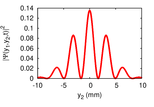
In the two-color ghost interference experiment, detector D1 is kept fixed and detector D2 is scanned along the y-axis. If we fix , the cosine term in (20) represents oscillations as a function of . This means that if particle 2 is detected in coincidence with a fixed D1, it will show an interference. The exponential terms represent overall Gaussian envelope on the interference pattern. The expression (20) should correctly describe the two-color ghost interference. The probability density given by (20), when plotted against the position of D2, yields an interference pattern (see Fig. 3). The fringe width of the pattern for particle 2 is given by
| (23) |
For , we get a simplified double-slit interference formula,
| (24) |
For we recover the familiar Young’s double-slit interference formula , which was obtained for the original ghost interference experiment [8], with being the strange distance between the double-slit and D2. For , (24) represents the fringe-width of the ghost interference for photon 2 which strangely also depends on the wavelength of photon 1.
3.2 Understanding ghost interference
Although entanglement between the two photons leads to a virtual double-slit formation for photon 2, that itself is not enough to yield ghost interference, just as a real double-slit for photon 1 does not yield an interference. By virtue of entanglement the two photons are spatially correlated - each one carries a which-way information about the other. By detecting photons 1 by a fixed D1, in the region where the wave-packets from the two slits overlap, one erases the which-way information. Once the which-way information has been erased, interference can occur [33, 34]. Thus, the two-color ghost interference is seen only when the photons 2 are detected in coincidence with a fixed D1.
Although the virtual double-slit for particle 2 comes into being only after particle 2 travels a distance from the source, the particle carries with itself the phase information of its evolution from the source for the time . Because of coincident counting, the change in phase because of the evolution of particle 1 is added to that of particle 2. This is what leads to the unusual fringe-width given by (24).
3.3 Effect of converging lens
Since Ding et al. [12] have used a converging lens before the detector D2, the fringe-width formula given by (24) doesn’t directly apply. However, if this experiment is done without the converging lens, the formula (24) can be experimentally tested.
It may be worthwhile to incorporate the effect of a coverging lens in our theoretical analysis, and see how the results are modified. This will allow us to make contact with Ding et al.’s experimental results. In order to do that, we consider the experimental setup similar to that of Ding et al. [12] (see Fig. 4).

A converging lens of focal length is kept at distance before detector D2. Consequently, the distance between the source and the lens is .
In our preceding calculation, particles 1 and 2 travel a distance so that particle 1 passes through the double-slit. Immediately after this the two-particle state is given by eqn. (15). The situation in this case is exactly the same, hence (15) still holds. However, after this, instead of travelling a distance to reach D2, particle 2 now travels a distance to reach the lens. The two-particle state at this time can be easily computed to yield
| (25) | |||||
where
| (26) |
and . Here we have used rescaled wavelengths .
The effect of a convegring lens on a general Gaussian wave-packet is such that in its subsequent dynamics, it narrows instead of spreading. If a Gaussian wave-packet of width starts from a distance from the lens, it should come back to its original width after a distance after the lens. Also, the observed width of the wavepacket, immediately after emerging from the lens should be the same as that just before entering the lens. In general, we can quantify the effect of the lens by a unitary transformation of the form [35]
where is the distance the wave-packet, of an initial width , traveled before passing through the lens, and is such that it satisfies
| (28) |
We make this transformation on the state (25) and let it evolve such that particle 2 travels a distance to reach D2. The probability density of finding particle 1 at and particle 2 at is given by
| (29) | |||||
where , ,
,
,
and
While arriving at this result, we have ignored the change in which
was expected from (28), because it does not affect the quantities
of our interest.
For , we get a simplified double-slit interference formula,
| (30) |
Eqn. (30) shows that the fringe width will be reduced after inserting a converging lens. Ding et al.’s experimental results can be analyzed using this formula. However, Ding et al. have not mentioned the values of etc, but have carried out a simple geometrical analysis. There is reasonable numerical agreement between Ding et al.’s simple geometrical analysis and their experimental results. However, we believe that their experimental results analyzed using eqn. (30) will give a better agreement.
We also emphasize that formulas (24, 30) are a signature of non-classical correlations between photons. An experimental verification of them would corroborate the non-classical origin of the two-color ghost interference. For this, the two-color ghost interference experiment should preferably be carried out without the converging lens. In addition, the detector D1 should be as narrow as D2, to prominently bring out the correlation between photons. In Ding et al.’s experiment, D1 is a bucket detector with width 1 mm, whereas D2 is a point detector with width 0.2 mm [12]. From the point of view of our calculation, having a bucket detector at D1 would amount to averaging over a range of values of in (29) or (20).
4 Conclusion
To summarize, we have theoretically analyzed the two-color ghost interference experiment, in a slightly more general setting. We find that the fringe width of the interference pattern for photon 2, also depends on the wavelength of photon 1. This is a completely non-classical feature. With a slight modification of the experiment, this conclusion can be experimentally tested. Its confirmation would be an evidence of the non-classical origin of the two-color ghost interference.
Acknowledgements.
This work was carried out during a summer project at the Centre for Theoretical Physics, Jamia Millia Islamia. Sheeba Shafaq thanks the Centre for providing her the facilities of the centre during the course of the summer project.References
- (1) A. Einstein, B. Podolsky, N. Rosen, Phys. Rev. 47, 777-780 (1935).
- (2) D. V. Strekalov, A. V. Sergienko, D. N. Klyshko, and Y. H. Shih, Phys. Rev. Lett. 74, 3600 (1995).
- (3) M. D’Angelo, Y-H. Kim, S. P. Kulik and Y. Shih, Phys. Rev. Lett. 92, 233601 (2004).
- (4) S. Thanvanthri and M. H. Rubin, Phys. Rev. A 70, 063811 (2004).
- (5) Y-H. Zhai, X-H. Chen, D. Zhang, L-A. Wu, Phys. Rev. A 72, 043805. (2005).
- (6) L. Jie, C. Jing, Chinese Phys. Lett. 28, 094203 (2011).
- (7) J. Kofler, M. Singh, M. Ebner, M. Keller, M. Kotyrba, A. Zeilinger, Phys. Rev. A 86, 032115 (2012).
- (8) P. Chingangbam, T. Qureshi, Prog. Theor. Phys. 127, 383-392 (2012).
- (9) S. Du, P. Kolchin, C. Belthangady, G. Y. Yin, and S. E. Harris, Phys. Rev. Lett. 100, 183603 (2008).
- (10) Q. F. Chen, B. S. Shi, M. Feng, Y. S. Zhang, and G. C. Guo, Opt. Express. 16, 21708 (2008).
- (11) X. S. Lu, Q. F. Chen, B. S. Shi, and G. C. Guo, Chin. Phys. Lett. 26, 064204 (2009).
- (12) D-S. Ding, Z-Y. Zhou, B-S. Shi, X-B Zou, G-C. Guo, AIP Advances 2, 032177 (2012).
- (13) T.B. Pittman, Y.H. Shih, D.V. Strekalov, A.V. Sergienko, Phys. Rev. A 52, R3429 (1995).
- (14) R.S. Bennink, S.J. Bentley, R.W Boyd, Phys. Rev. Lett. 89, 113601 (2002).
- (15) R.S. Bennink, S.J. Bentley, R.W. Boyd, J.C. Howell, Phys. Rev. Lett. 92, 033601 (2004).
- (16) A. Gatti, E. Brambilla, L.A. Lugiato, Phys. Rev. Lett. 90, 133603 (2003).
- (17) A. Gatti, E. Brambilla, M. Bache, L.A. Lugiato, Phys. Rev. A 70, 013802 (2004).
- (18) A. Gatti, E. Brambilla, M. Bache, L.A. Lugiato, Phys. Rev. Lett. 93, 093602 (2004).
- (19) A. Valencia, G. Scarcelli, M. D’Angelo, Y. Shih, Phys. Rev. Lett. 94, 063601 (2005).
- (20) F. Ferri, D. Magatti, A. Gatti, M. Bache, E. Brambilla, L.A. Lugiato, Phys. Rev. Lett. 94, 183602 (2005).
- (21) J. Cheng, S. Han, Phys. Rev. Lett. 92, 093903 (2004).
- (22) Y. Bai, S. Han, Opt. Comm. 280, 393-396 (2007).
- (23) L. Basano, P. Ottonello, Opt. Commun. 282, 2741-2745 (2009).
- (24) M.H. Rubin, Y. Shih, Phys. Rev. A 78, 033836 (2008).
- (25) K.W.C. Chan, M.N. O’Sullivan, R.W. Boyd, Phys. Rev. A 79, 033808 (2009).
- (26) S. Karmakar, Y. Shih, Proc. SPIE 7815, 78150R (2010).
- (27) G. Scarcelli, V. Berardi, Y. Shih, Phys. Rev. Lett. 96, 063602 (2006).
- (28) J.H. Shapiro, R.W. Boyd, Quantum Inf. Process. 11, 949-993 (2012).
- (29) Y. Shih, Quantum Inf. Process. 11, 995-1001, (2012).
- (30) J.H. Shapiro, R.W. Boyd, Quantum Inf. Process. 11, 1003-1011, (2012).
- (31) I. Neder, M. Heiblum, D. Mahalu, V. Umansky, Phys. Rev. Lett. 98 (2007), 036803.
- (32) L. Mandel and E. Wolf, Optical Coherence and Quantum Optics (Cambridge, University Press, 1995).
- (33) M. O. Scully and K. Drühl, Phys. Rev. A 25, 2208 (1982).
- (34) E. Jaynes, in Foundations of Radiation Theory and Quantum Electronics, ed. A. O. Barut (Plenum, New York 1980), pp. 37.
- (35) T. Qureshi, Prog. Theor. Phys. 127, 645 (2012).