跳到论文正文
W Papers独立论文阅读器 arXiv:1308.4529 论文正文 计算阅读时间 · 0%
引用这篇论文根据当前论文元数据生成,正式投稿前建议核对。


License: arXiv.org perpetual non-exclusive license
arXiv:1308.4529v2 [math.NA] 24 Aug 2014

Higher order strong approximations of semilinear stochastic wave equation with additive space-time white noise Thanks: This work was supported by NSF of China (No.11301550 and No.11171352) and China Postdoctoral Science Foundation (No.2013M531798 and No.2014T70779).

Xiaojie Wang ††thanks: School of Mathematics and Statistics, and School of Geosciences and Info-Physics, Central South University, Changsha 410083, Hunan, China (x.j.wang7@gmail.com, x.j.wang7@csu.edu.cn).    Siqing Gan ††thanks: School of Mathematics and Statistics, Central South University, Changsha 410083, Hunan, China (sqgan@csu.edu.cn).    Jingtian Tang ††thanks: School of Geosciences and Info-Physics, Central South University, Changsha 410083, Hunan, China (jttang@csu.edu.cn).
Abstract

Novel fully discrete schemes are developed to numerically approximate a semilinear stochastic wave equation driven by additive space-time white noise. Spectral Galerkin method is proposed for the spatial discretization, and exponential time integrators involving linear functionals of the noise are introduced for the temporal approximation. The resulting fully discrete schemes are very easy to implement and allow for higher strong convergence rate in time than existing time-stepping schemes such as the Crank-Nicolson-Maruyama scheme and the stochastic trigonometric method. Particularly, it is shown that the new schemes achieve in time an order of 1−ϵ1-\epsilon for arbitrarily small ϵ>0\epsilon>0, which exceeds the barrier order 12\frac{1}{2} established by Walsh [32]. Numerical results confirm higher convergence rates and computational efficiency of the new schemes.

keywords
semilinear stochastic wave equation, space-time white noise, strong approximations, spectral Galerkin method, exponential time integrator
AMS
60H35, 60H15, 65C30

1 Introduction

Wave motions and mechanical vibrations are two common physical phenomena that are usually modeled by hyperbolic partial differential equations. In many practical applications, random perturbation occurs and a noisy force term is hence included in the model problems. This leads to stochastic partial differential equations (SPDEs) of hyperbolic type [4, 31]. One of the fundamental hyperbolic SPDEs is the stochastic wave equation, which describes a variety of physical processes, such as the motion of a vibrating string [1] and the motion of a strand of DNA [6].

The present work deals with the strong approximations (cf. [19]) of the semilinear stochastic wave equation (SWE) driven by additive space-time white noise,

{∂2u∂t2=∂2u∂x2+f(x,u)+W˙,t∈(0,T],x∈(0,1),u(0,x)=u0(x),∂u∂t(0,x)=v0(x),x∈(0,1),u(t,0)=u(t,1)=0,t>0,\left\{\begin{array}[]{lll}\frac{\partial^{2}u}{\partial t^{2}}=\frac{\partial^{2}u}{\partial x^{2}}+f(x,u)+\dot{W},\quad t\in(0,T],\>\>x\in(0,1),\\ u(0,x)=u_{0}(x),\,\frac{\partial u}{\partial t}(0,x)=v_{0}(x),\>x\in(0,1),\\ u(t,0)=u(t,1)=0,\>t>0,\end{array}\right. (1)

where T∈(0,∞)T\in(0,\infty) and f:[0,1]×ℝ→ℝf\colon[0,1]\times\mathbb{R}\rightarrow\mathbb{R} is a smooth nonlinear function satisfying

|f⁡(x,z)|≤\displaystyle|f(x,z)|\leq L⁡(|z|+1),\displaystyle L(|z|+1), (2)
|∂f∂z​(x,z)|≤L,|∂2f∂x​∂z​(x,z)|\displaystyle\big|\tfrac{\partial f}{\partial z}(x,z)\big|\leq L,\quad\big|\tfrac{\partial^{2}f}{\partial x\partial z}(x,z)\big| ≤L,and|∂2f∂z2​(x,z)|≤L\displaystyle\leq L,\quad\mbox{and}\quad\big|\tfrac{\partial^{2}f}{\partial z^{2}}(x,z)\big|\leq L (3)

for all x∈[0,1],z∈ℝx\in[0,1],\,z\in\mathbb{R} and some constant L>0L>0. The initial data u0u_{0} and v0v_{0} are random variables that will be specified later. The forcing term W˙\dot{W} is a space-time white noise (see below), which best models the fluctuations generated by microscopic effects in a homogeneous physical system [9].

In recent years, much progress has been made in both strong and weak approximations of parabolic SPDEs, see [15, 16, 23, 24] and the references therein. In contrast to the parabolic case, there exist only a very limited number of works devoted to the numerical study of stochastic wave equations [2, 5, 12, 20, 21, 22, 25, 27, 28, 32]. In [27], a finite difference method was considered for spatial semi-discretizations of SWE subject to multiplicative space-time white noise and a strong convergence rate of order 13\tfrac{1}{3} was obtained. The convergence rate was improved from 13\frac{1}{3} to 12−ϵ\frac{1}{2}-\epsilon for arbitrarily small ϵ>0\epsilon>0 in [2] by using a spectral Galerkin method in spatial approximation of SWE with additive noise. Using an adaptation of “leapfrog” discretization, Walsh [32] constructed a (fully discrete) finite difference scheme, which attains convergence order 12\tfrac{1}{2} in both time and space. In a series of works on numerical analysis of linear stochastic evolution equations with additive noise [20, 21, 22], spatial approximations by finite element methods and temporal discretizations by rational approximations to the exponential function have been investigated. For the case of space-time white noise, the strong convergence results in [20, 22] (Theorem 5.1 in [20] and Theorem 4.6 in [22]) imply convergence rates of rr+1​β\tfrac{r}{r+1}\beta in space and pp+1​β\tfrac{p}{p+1}\beta in time, for β<12\beta<\tfrac{1}{2} and p,r∈ℕ+p,r\in\mathbb{N}^{+} being method parameters. Recently in [5], a stochastic trigonometric method was introduced for the temporal approximation of linear SWEs, which strongly converges with order 12−ϵ\tfrac{1}{2}-\epsilon for arbitrary small ϵ>0\epsilon>0 in the space-time white noise case (see Theorem 4.1 in [5]).

To the best of our knowledge, we have not found any numerical method that strongly converges with a rate faster than 12\tfrac{1}{2} in the literature. This seems to be an order barrier. In fact, the limit on the convergence rate of numerical schemes for SWEs driven by space-time white noise, has been established [32] in the sense that no scheme based on the basic increments of white noise strongly converges at a rate faster than 12\tfrac{1}{2}. An interesting question thus arises as to whether it is possible to overcome the order barrier. In this work, we provide a positive answer to this question by designing two fully discrete schemes for the SWE (1), which enjoy a strong convergence order greater than 12\tfrac{1}{2}. More precisely, we spatially discretize (1) by a spectral Galerkin method, and then propose two exponential time integrators involving two linear functionals of the noise. As shown in the main convergence result (Theorem 5), under the conditions (2) and (3) the proposed fully discrete schemes strongly converge with order 12−ϵ\tfrac{1}{2}-\epsilon in space and order 1−ϵ1-\epsilon in time for arbitrarily small ϵ>0\epsilon>0. Compared with existing schemes mentioned earlier, the proposed schemes are easy to implement and produce significant improvement on the computational efficiency (see Section 5).

Finally, we mention that the idea of using linear functionals of the noise process in time-stepping schemes was exploited in [14, 17] to approximate semilinear stochastic heat equations with additive noise. In [14], a so-called accelerated exponential Euler (AEE) method [7] is shown to strongly converge with order 1−ϵ1-\epsilon under seriously restrictive commutativity assumptions (see Assumption 2.4 in [14] and discussion in the introduction of [17]). In the present work, such AEE method is successfully adapted to solve the SWE (1) and under standard assumptions the strong convergence rate of order 1−ϵ1-\epsilon in time is proved in the space-time white noise case.

The rest of this paper is organized as follows. In the next section, some preliminaries are collected and an abstract formulation of (1) is set forth. In Section 3, we analyze the strong approximation error arising from the spatial discretization by a spectral Galerkin method. Then two exponential time integrators are introduced and strong convergence of the fully discrete approximations are studied in Section 4. Numerical experiments confirming our theoretical results are presented in Section 5. The paper is concluded with some brief remarks in Section 6.

2 Preliminaries and framework

Let (U,⟨⋅,⋅⟩,∥⋅∥)(U,\,\langle\cdot,\cdot\rangle,\,\|\cdot\|) and (H,(⋅,⋅),∥|⋅∥|)(H,\,(\cdot,\cdot),\,\||\cdot\||) be two separable Hilbert spaces. By ℒ⁡(U,H)\mathcal{L}(U,H) we denote the Banach space of bounded linear operators from UU to HH and for short we write ℒ⁡(U):=ℒ⁡(U,U)\mathcal{L}(U):=\mathcal{L}(U,U). Additionally, we need the Banach space of Hilbert-Schmidt operators, denoted by ℒ2​(U,H)\mathcal{L}_{2}(U,H), equipped with the norm

∥Γ∥ℒ2​(U,H)=(∑i=1∞∥|Γηi∥|2)1/2,\|\Gamma\|_{\mathcal{L}_{2}(U,H)}=\Big(\sum_{i=1}^{\infty}\||\Gamma\eta_{i}\||^{2}\Big)^{1/2}, (4)

where {ηi}i∈ℕ\{\eta_{i}\}_{i\in\mathbb{N}} is an orthonormal basis of UU and the norm does not depend on the particular choice of the basis [8, 26]. For brevity, we write ℒ2​(U):=ℒ2​(U,U)\mathcal{L}_{2}(U):=\mathcal{L}_{2}(U,U). If Γ1∈ℒ⁡(U,H)\Gamma_{1}\in\mathcal{L}(U,H) and Γ2∈ℒ2​(U)\Gamma_{2}\in\mathcal{L}_{2}(U), then Γ1​Γ2∈ℒ2​(U,H)\Gamma_{1}\Gamma_{2}\in\mathcal{L}_{2}(U,H), and

‖Γ1​Γ2‖ℒ2​(U,H)≤‖Γ1‖ℒ⁡(U,H)⋅‖Γ2‖ℒ2​(U).\|\Gamma_{1}\Gamma_{2}\|_{\mathcal{L}_{2}(U,H)}\leq\|\Gamma_{1}\|_{\mathcal{L}(U,H)}\cdot\|\Gamma_{2}\|_{\mathcal{L}_{2}(U)}. (5)

Let (Ω,ℱ,ℙ)\left(\Omega,\mathcal{F},\mathbb{P}\right) be a probability space with a normal filtration {ℱt}0≤t≤T\{\mathcal{F}_{t}\}_{0\leq t\leq T} and by Lp​(Ω,U)L^{p}(\Omega,U) we denote the space of UU-valued integrable random variables with the norm defined by ‖φ‖Lp​(Ω,U)=(𝔼⁡[‖φ‖p])1p<∞\|\varphi\|_{L^{p}(\Omega,U)}=\big(\mathbb{E}\big[\|\varphi\|^{p}\big]\big)^{\frac{1}{p}}<\infty for any p≥2p\geq 2.

Next, we take U:=L2​((0,1),ℝ)U:=L^{2}\big((0,1),\mathbb{R}\big) to denote the space of real-valued square integrable functions, equipped with the usual norm ∥⋅∥\|\cdot\| and inner product ⟨⋅,⋅⟩\langle\cdot,\cdot\rangle. Let −Λ=Δ:𝒟⁡(Λ)⊂U→U-\Lambda=\Delta:\mathcal{D}(\Lambda)\subset U\rightarrow U be the Laplace operator with 𝒟⁡(Λ)=H2​(0,1)∩H01​(0,1)\mathcal{D}(\Lambda)=H^{2}(0,1)\cap H_{0}^{1}(0,1), where Hm​(0,1)H^{m}(0,1) denote the standard Sobolev spaces of integer order m≥1m\geq 1 and H01​(0,1):={φ∈H1​(0,1):φ⁡(0)=φ⁡(1)=0}H_{0}^{1}(0,1):=\{\varphi\in H^{1}(0,1)\colon\varphi(0)=\varphi(1)=0\}. Then Λ\Lambda is a densely defined, self-adjoint, positive operator with compact inverse. Moreover, the eigenvalue problem

Λ​ei=λi​ei,i∈ℕ\Lambda e_{i}=\lambda_{i}e_{i},\,i\in\mathbb{N} (6)

provides an orthonormal basis {ei=2​sin⁡(i​π​x),x∈(0,1)}i∈ℕ\{e_{i}=\sqrt{2}\sin(i\pi x),\,x\in(0,1)\}_{i\in\mathbb{N}} for UU and an increasing sequence of eigenvalues λi=π2​i2,i∈ℕ\lambda_{i}=\pi^{2}i^{2},i\in\mathbb{N}. Additionally, let F:U→UF:U\rightarrow U be a Nemytskij operator associated to ff as in (1), defined by

F⁡(φ)​(x)=f⁡(x,φ⁡(x)),x∈(0,1),φ∈U.F(\varphi)(x)=f(x,\varphi(x)),\quad x\in(0,1),\>\varphi\in U. (7)

Now one can rewrite (1) as an abstract form in Itô’s sense

{du˙=−Λudt+F(u)dt+dW(t),t∈(0,T],u(0)=u0,u˙(0)=v0,\displaystyle\left\{\!\begin{array}[]{ll}\mbox{d}\dot{u}=-\Lambda u\mbox{d}t+F(u)\mbox{d}t+\mbox{d}W(t),\quad t\in(0,T],\\ u(0)=u_{0},\,\dot{u}(0)=v_{0},\end{array}\right.

where uu is regarded as a UU-valued stochastic process and u˙\dot{u} stands for the time derivative of uu. The driven stochastic process W⁡(t)W(t) is a cylindrical II-Wiener process with respect to {ℱt}0≤t≤T\{\mathcal{F}_{t}\}_{0\leq t\leq T}, which can be represented as follows [8, 26]:

W⁡(t)=∑i=1∞βi​(t)​ei,t∈[0,T],\displaystyle W(t)=\sum_{i=1}^{\infty}\beta_{i}(t)e_{i},\quad t\in[0,T], (10)

where {βi​(t)}i∈ℕ\{\beta_{i}(t)\}_{i\in\mathbb{N}} are independent real-valued Brownian motions and {ei}i∈ℕ\{e_{i}\}_{i\in\mathbb{N}} are the eigenvectors of Λ\Lambda defined by (6). Moreover, note that the derivative operators of FF are given by

F′​(φ)​(ψ)​(x)=\displaystyle F^{\prime}(\varphi)(\psi)\,(x)= ∂f∂z​(x,φ⁡(x))⋅ψ⁡(x),x∈(0,1),\displaystyle\tfrac{\partial f}{\partial z}(x,\varphi(x))\cdot\psi(x),\quad x\in(0,1), (11)
F′′​(φ)​(ψ1,ψ2)​(x)=\displaystyle F^{\prime\prime}(\varphi)(\psi_{1},\psi_{2})\,(x)= ∂2f∂z2​(x,φ⁡(x))⋅ψ1​(x)⋅ψ2​(x),x∈(0,1),\displaystyle\tfrac{\partial^{2}f}{\partial z^{2}}(x,\varphi(x))\cdot\psi_{1}(x)\cdot\psi_{2}(x),\quad x\in(0,1), (12)

for all φ,ψ,ψ1,ψ2∈U\varphi,\psi,\psi_{1},\psi_{2}\in U. It is worthwhile to keep in mind that the derivative operators F′​(φ),F′′​(φ),φ∈UF^{\prime}(\varphi),F^{\prime\prime}(\varphi),\varphi\in U defined in the above way are self-adjoint. Thanks to (2) and (3), the Nemytskij operator FF satisfies

‖F⁡(φ)‖≤\displaystyle\|F(\varphi)\|\leq 2​L​(‖φ‖+1),\displaystyle\sqrt{2}L(\|\varphi\|+1), (13)
‖F⁡(φ1)−F⁡(φ2)‖≤\displaystyle\|F(\varphi_{1})-F(\varphi_{2})\|\leq L​‖φ1−φ2‖\displaystyle L\|\varphi_{1}-\varphi_{2}\| (14)

for all φ,φ1,φ2∈U\varphi,\varphi_{1},\varphi_{2}\in U. Also, it is obvious that

‖Λβ−12‖ℒ2​(U)2=∑i=1∞‖Λβ−12​ei‖2=∑i=1∞π2​(β−1)i2​(1−β)≤c¯β<∞,for any ​β<12.\displaystyle\big\|\Lambda^{\frac{\beta-1}{2}}\big\|^{2}_{\mathcal{L}_{2}(U)}=\sum_{i=1}^{\infty}\|\Lambda^{\frac{\beta-1}{2}}e_{i}\|^{2}=\sum_{i=1}^{\infty}\frac{\pi^{2(\beta-1)}}{i^{2(1-\beta)}}\leq\bar{c}_{\beta}<\infty,\quad\mbox{for any }\beta<\tfrac{1}{2}. (15)

In order to define the mild solution of (2) appropriately, we shall reformulate (2) as a stochastic evolution equation in a new Hilbert space HH to fall into the semigroup framework in [8]. To this end, we need additional spaces and notations. The above setting enables us to define fractional powers of Λ\Lambda in a simple way (see, e.g., [23, Appendix B.2]). Accordingly, we introduce the separable Hilbert space H˙α:=𝒟⁡(Λα2)\dot{H}^{\alpha}:=\mathcal{D}(\Lambda^{\frac{\alpha}{2}}), α∈ℝ\alpha\in\mathbb{R}, equipped with the inner product

⟨φ,ψ⟩α:=⟨Λα2​φ,Λα2​ψ⟩=∑i=1∞λiα​⟨φ,ei⟩​⟨ψ,ei⟩,φ,ψ∈H˙α,\langle\varphi,\psi\rangle_{\alpha}:=\langle\Lambda^{\frac{\alpha}{2}}\varphi,\Lambda^{\frac{\alpha}{2}}\psi\rangle=\sum_{i=1}^{\infty}\lambda_{i}^{\alpha}\langle\varphi,e_{i}\rangle\langle\psi,e_{i}\rangle,\quad\varphi,\psi\in\dot{H}^{\alpha}, (16)

where {(λi,ei)}i=1∞\{(\lambda_{i},e_{i})\}_{i=1}^{\infty} are the eigenpairs of Λ\Lambda. The corresponding norm is defined by ‖φ‖α=⟨φ,φ⟩α\|\varphi\|_{\alpha}=\sqrt{\langle\varphi,\varphi\rangle_{\alpha}} for φ∈H˙α\varphi\in\dot{H}^{\alpha}. Then H˙0=U\dot{H}^{0}=U and H˙α⊂H˙β\dot{H}^{\alpha}\subset\dot{H}^{\beta} if α≥β\alpha\geq\beta. Moreover, H˙−γ\dot{H}^{-\gamma} can be identified with the dual space (H˙γ)∗\big(\dot{H}^{\gamma}\big)^{*} for γ>0\gamma>0 [29]. Further, we introduce the product space Hα:=H˙α×H˙α−1H^{\alpha}:=\dot{H}^{\alpha}\times\dot{H}^{\alpha-1}, α∈ℝ\alpha\in\mathbb{R}, endowed with the inner product

(Y,Y^)α:=⟨φ,φ^⟩α+⟨ψ,ψ^⟩α−1,Y=(φ,ψ)T,Y^=(φ^,ψ^)T,(Y,\hat{Y})_{\alpha}:=\langle\varphi,\hat{\varphi}\rangle_{\alpha}+\langle\psi,\hat{\psi}\rangle_{\alpha-1},\quad Y=(\varphi,\psi)^{T},\>\hat{Y}=(\hat{\varphi},\hat{\psi})^{T}, (17)

and the usual norm

∥|Y∥|α2:=∥φ∥α2+∥ψ∥α−12,Y=(φ,ψ)T.\displaystyle\||Y\||_{\alpha}^{2}:=\|\varphi\|_{\alpha}^{2}+\|\psi\|^{2}_{\alpha-1},\quad Y=(\varphi,\psi)^{T}. (18)

It is easy to check that (Hα,(⋅,⋅)α)(H^{\alpha},\,(\cdot,\cdot)_{\alpha}), α∈ℝ\alpha\in\mathbb{R}, is a separable Hilbert space. For the special case α=0\alpha=0, we denote H:=H0=H˙0×H˙−1H:=H^{0}=\dot{H}^{0}\times\dot{H}^{-1}, (⋅,⋅):=(⋅,⋅)0(\cdot,\cdot):=(\cdot,\cdot)_{0}, and ∥|⋅∥|:=∥|⋅∥|0\||\cdot\||:=\||\cdot\||_{0}.

At this point, we introduce the velocity of the solution uu, denoted by v=u˙v=\dot{u}, and formally transform (2) into the following Cauchy problem

{dX(t)=AX(t)dt+𝐅(X)dt+BdW(t),t∈(0,T],X⁡(0)=X0,\left\{\begin{array}[]{ll}\mbox{d}X(t)=AX(t)\mbox{d}t+\mathbf{F}(X)\mbox{d}t+B\mbox{d}W(t),\quad t\in(0,T],\\ X(0)=X_{0},\end{array}\right. (19)

where X0=(u0,v0)TX_{0}=(u_{0},v_{0})^{T} and

X=[uv],A=[0I−Λ0],𝐅⁡(X)=[0F⁡(u)],B=[0I].X=\bigg[\!\begin{array}[]{c}u\\ v\end{array}\!\bigg],\>A=\bigg[\!\begin{array}[]{cc}0&I\\ -\Lambda&0\end{array}\!\bigg],\>\mathbf{F}(X)=\bigg[\!\begin{array}[]{c}0\\ F(u)\end{array}\!\bigg],\>B=\bigg[\!\begin{array}[]{c}0\\ I\end{array}\!\bigg]. (20)

Here X0X_{0} is assumed to be an ℱ0\mathcal{F}_{0}-measurable HH-valued random variable and BB is considered as an operator from H˙−1\dot{H}^{-1} to HH. From now on, we regard Λ\Lambda as an operator from H˙1\dot{H}^{1} to H˙−1\dot{H}^{-1}, defined by (Λ​φ)​(ψ)=⟨∇φ,∇ψ⟩(\Lambda\varphi)(\psi)=\langle\nabla\varphi,\nabla\psi\rangle for φ,ψ∈H˙1\varphi,\psi\in\dot{H}^{1} and define the domain of AA by

𝒟⁡(A)={Y=(φ,ψ)T∈H:A​Y=[ψ−Λ​φ]∈H=H˙0×H˙−1}=H1=H˙1×H˙0.\mathcal{D}(A)=\bigg\{Y=(\varphi,\psi)^{T}\in H:AY=\bigg[\!\begin{array}[]{c}\psi\\ -\Lambda\varphi\end{array}\!\bigg]\in H=\dot{H}^{0}\times\dot{H}^{-1}\bigg\}=H^{1}=\dot{H}^{1}\times\dot{H}^{0}.

Then the operator AA is the generator of a strongly continuous semigroup E⁡(t),t≥0E(t),t\geq 0 on HH [24, Section 5.3], that can be written as

E⁡(t)=et​A=[C⁡(t)Λ−12​S​(t)−Λ12​S​(t)C⁡(t)].\displaystyle E(t)=e^{tA}=\left[\!\begin{array}[]{cc}C(t)&\Lambda^{-\frac{1}{2}}S(t)\\ -\Lambda^{\frac{1}{2}}S(t)&C(t)\end{array}\!\right].

Here C⁡(t)=cos⁡(t​Λ12)C(t)\!=\!\cos(t\Lambda^{\frac{1}{2}}) and S⁡(t)=sin⁡(t​Λ12)S(t)\!=\!\sin(t\Lambda^{\frac{1}{2}}) are the so-called cosine and sine operators, which can be expressed in terms of the eigenpairs {λi,ei}i∈ℕ\{\lambda_{i},e_{i}\}_{i\in\mathbb{N}}:

C⁡(t)​φ=∑i=1∞cos⁡(t​λi1/2)​⟨φ,ei⟩​ei,S⁡(t)​φ=∑i=1∞sin⁡(t​λi1/2)​⟨φ,ei⟩​ei\displaystyle C(t)\varphi=\sum_{i=1}^{\infty}\cos(t\lambda_{i}^{1/2})\langle\varphi,e_{i}\rangle e_{i},\quad S(t)\varphi=\sum_{i=1}^{\infty}\sin(t\lambda_{i}^{1/2})\langle\varphi,e_{i}\rangle e_{i}

for t≥0,φ∈H˙−1t\geq 0,\varphi\in\dot{H}^{-1}. Before proceeding further, we briefly state some properties of C⁡(t)C(t) and S⁡(t)S(t), which will be used frequently later. As defined above, the cosine and sine operators are bounded in the sense that ‖C⁡(t)​φ‖≤‖φ‖\|C(t)\varphi\|\leq\|\varphi\| and ‖S⁡(t)​φ‖≤‖φ‖\|S(t)\varphi\|\leq\|\varphi\| hold for all φ∈U\varphi\in U. In addition, these two operators satisfy the trigonometric identity ‖S⁡(t)​φ‖2+‖C⁡(t)​φ‖2=‖φ‖2\|S(t)\varphi\|^{2}+\|C(t)\varphi\|^{2}=\|\varphi\|^{2} for φ∈U\varphi\in U. Moreover, Λγ\Lambda^{\gamma}, γ∈ℝ\gamma\in\mathbb{R} commutes with C⁡(t),S⁡(t)C(t),S(t) since they are all defined in terms of the eigenbasis {ei}i∈ℕ\{e_{i}\}_{i\in\mathbb{N}}. With the aid of these properties together, one can show that ∥|E(t)Y∥|γ≤∥|Y∥|γ\||E(t)Y\||_{\gamma}\leq\||Y\||_{\gamma} for t∈[0,∞),γ∈ℝ,Y∈Hγt\in[0,\infty),\gamma\in\mathbb{R},Y\in H^{\gamma}. Now, we look at the existence and uniqueness of the mild solution of (19), which has been discussed in [3, 27] using different frameworks.

Theorem 1.

Suppose conditions (2) and (3) are fulfilled, let W⁡(t),t∈[0,T]W(t),t\in[0,T] be the cylindrical II-Wiener process represented by (10), and let X0X_{0} be an ℱ0\mathcal{F}_{0}-measurable HH-valued random variable satisfying ‖X0‖Lp​(Ω,H)<∞\|X_{0}\|_{L^{p}(\Omega,H)}<\infty for some p≥2p\geq 2. Then SWE (19) has a unique mild solution given by

X⁡(t)=E⁡(t)​X0+∫0tE⁡(t−s)​𝐅​(X⁡(s))​d​s+∫0tE⁡(t−s)​B​d​W​(s)​a.s.\displaystyle\small X(t)=E(t)X_{0}+\int_{0}^{t}E(t-s)\mathbf{F}(X(s))\,\mbox{d}s+\int_{0}^{t}E(t-s)B\,\mbox{d}W(s)\hskip 9.24994pta.s. (23)

for each t∈[0,T]t\in[0,T]. Additionally, if ‖X0‖Lp​(Ω,H1/2)<∞\|X_{0}\|_{L^{p}(\Omega,H^{1/2})}<\infty then there exists a constant K1​(p,β,T)∈[0,∞)K_{1}(p,\beta,T)\in[0,\infty) depending on p,β,Tp,\beta,T such that for any 0≤β<120\leq\beta<\frac{1}{2}

supt∈[0,T]‖X⁡(t)‖Lp​(Ω,Hβ)≤K1​(‖X0‖Lp​(Ω,Hβ)+1).\displaystyle\sup_{t\in[0,T]}\|X(t)\|_{L^{p}(\Omega,H^{\beta})}\leq K_{1}\big(\|X_{0}\|_{L^{p}(\Omega,H^{\beta})}+1\big). (24)

Proof. We first claim that the nonlinear operator 𝐅:H→H\mathbf{F}\colon H\rightarrow H satisfies the globally Lipschitz condition and linear growth condition. In fact, for any Y=(φ,ψ)T∈HY=(\varphi,\psi)^{T}\in H, Y1=(φ1,ψ1)T∈HY_{1}=(\varphi_{1},\psi_{1})^{T}\in H, Y2=(φ2,ψ2)T∈HY_{2}=(\varphi_{2},\psi_{2})^{T}\in H, we infer

∥|𝐅(Y1)−𝐅(Y2)∥|=\displaystyle\||\mathbf{F}(Y_{1})-\mathbf{F}(Y_{2})\||= ∥Λ−12(F(φ1)−F(φ2))∥≤L∥φ1−φ2∥≤L∥|Y1−Y2∥|,\displaystyle\|\Lambda^{-\frac{1}{2}}\big(F(\varphi_{1})-F(\varphi_{2})\big)\|\leq L\|\varphi_{1}-\varphi_{2}\|\leq L\||Y_{1}-Y_{2}\||,
∥|𝐅(Y)∥|=\displaystyle\||\mathbf{F}(Y)\||= ∥Λ−12F(φ)∥≤2L(∥φ∥+1)≤2L(∥|Y∥|+1)\displaystyle\|\Lambda^{-\frac{1}{2}}F(\varphi)\|\leq\sqrt{2}L(\|\varphi\|+1)\leq\sqrt{2}L(\||Y\||+1)

by (13), (14), the definitions of 𝐅\mathbf{F} and ∥|⋅∥|\||\cdot\||, and stability of Λ−12\Lambda^{-\frac{1}{2}}. Here and below by “stability” of a linear operator Γ:U→U\Gamma\colon U\rightarrow U, we mean Γ\Gamma is bounded and satisfies ‖Γ​φ‖≤‖φ‖\|\Gamma\varphi\|\leq\|\varphi\| for all φ∈U\varphi\in U. Furthermore, we have

∥B∥ℒ2​(U,H)=(∑i=1∞∥|Bei∥|2)12=(∑i=1∞∥Λ−12ei∥2)12=(∑i=1∞λi−1)12<∞.\|B\|_{\mathcal{L}_{2}(U,H)}=\Big(\sum_{i=1}^{\infty}\||Be_{i}\||^{2}\Big)^{\frac{1}{2}}=\Big(\sum_{i=1}^{\infty}\|\Lambda^{-\frac{1}{2}}e_{i}\|^{2}\Big)^{\frac{1}{2}}=\Big(\sum_{i=1}^{\infty}\lambda_{i}^{-1}\Big)^{\frac{1}{2}}<\infty. (25)

In view of Theorem 7.4 from [8], one can derive the existence and uniqueness of the mild solution (23), which satisfies

supt∈[0,T]‖X⁡(t)‖Lp​(Ω,H)≤Cp,T​(‖X0‖Lp​(Ω,H)+1).\displaystyle\sup_{t\in[0,T]}\|X(t)\|_{L^{p}(\Omega,H)}\leq C_{p,T}\left(\|X_{0}\|_{L^{p}(\Omega,H)}+1\right). (26)

By using the trigonometric identity and (15) one can easily show that, for t∈[0,T]t\in[0,T]

∫0t‖E⁡(t−s)​B‖ℒ2​(U,Hβ)2​d​s≤t​‖Λβ−12‖ℒ2​(U)2≤t​c¯β<∞,β∈[0,12).\int_{0}^{t}\|E(t-s)B\|^{2}_{\mathcal{L}_{2}(U,H^{\beta})}\mbox{d}s\leq t\|\Lambda^{\frac{\beta-1}{2}}\|^{2}_{\mathcal{L}_{2}(U)}\leq t\bar{c}_{\beta}<\infty,\quad\beta\in[0,\tfrac{1}{2}). (27)

Using this together with (13), (18), the Burkholder-Davis-Gundy type inequality ([8, Lemma 7.2]) and some properties of the operators Λγ\Lambda^{\gamma}, γ∈ℝ\gamma\in\mathbb{R}, C⁡(t)C(t) and S⁡(t)S(t) mentioned earlier, we deduce from (23) that

‖X⁡(t)‖Lp​(Ω,Hβ)\displaystyle\|X(t)\|_{L^{p}(\Omega,H^{\beta})}
≤\displaystyle\leq ‖E⁡(t)​X0‖Lp​(Ω,Hβ)+∫0t‖E⁡(t−s)​𝐅​(X⁡(s))‖Lp​(Ω,Hβ)​d​s\displaystyle\|E(t)X_{0}\|_{L^{p}(\Omega,H^{\beta})}+\int_{0}^{t}\left\|E(t-s)\mathbf{F}(X(s))\right\|_{L^{p}(\Omega,H^{\beta})}\mbox{d}s
+‖∫0tE⁡(t−s)​B​d​W​(s)‖Lp​(Ω,Hβ)\displaystyle+\left\|\int_{0}^{t}E(t-s)B\,\mbox{d}W(s)\right\|_{L^{p}(\Omega,H^{\beta})}
≤\displaystyle\leq ∥∥|E(t)X0∥|β∥Lp​(Ω,ℝ)+cp(∫0t∥E(t−s)B∥ℒ2​(U,Hβ)2ds)12\displaystyle\big\|\||E(t)X_{0}\||_{\beta}\big\|_{L^{p}(\Omega,\mathbb{R})}\!+c_{p}\bigg(\!\int_{0}^{t}\|E(t-s)B\|^{2}_{\mathcal{L}_{2}(U,H^{\beta})}\mbox{d}s\!\bigg)^{\frac{1}{2}}
+∫0t∥(∥Λ−12S(t−s)F(u(s))∥β2+∥C(t−s)F(u(s))∥β−12)12∥Lp​(Ω,ℝ)ds\displaystyle+\int_{0}^{t}\Big\|\Big(\|\Lambda^{-\frac{1}{2}}S(t-s)F(u(s))\|^{2}_{\beta}+\|C(t-s)F(u(s))\|^{2}_{\beta-1}\Big)^{\frac{1}{2}}\Big\|_{L^{p}(\Omega,\mathbb{R})}\mbox{d}s
≤\displaystyle\leq ∥∥|X0∥|β∥Lp​(Ω,ℝ)+t​c¯βcp+∫0t∥∥F(u(s))∥β−1∥Lp​(Ω,ℝ)ds\displaystyle\big\|\||X_{0}\||_{\beta}\big\|_{L^{p}(\Omega,\mathbb{R})}+\sqrt{t\bar{c}_{\beta}}\,c_{p}+\int_{0}^{t}\big\|\,\|F(u(s))\|_{\beta-1}\big\|_{L^{p}(\Omega,\mathbb{R})}\mbox{d}s
≤\displaystyle\leq ‖X0‖Lp​(Ω,Hβ)+t​c¯β​cp+2​L​∫0t‖‖u⁡(s)‖+1‖Lp​(Ω,ℝ)​d​s\displaystyle\|X_{0}\|_{L^{p}(\Omega,H^{\beta})}+\sqrt{t\bar{c}_{\beta}}\,c_{p}+\sqrt{2}L\int_{0}^{t}\big\|\,\|u(s)\|+1\big\|_{L^{p}(\Omega,\mathbb{R})}\mbox{d}s
≤\displaystyle\leq ‖X0‖Lp​(Ω,Hβ)+t​c¯β​cp+2​L​t+2​L​∫0t‖u⁡(s)‖Lp​(Ω,U)​d​s\displaystyle\|X_{0}\|_{L^{p}(\Omega,H^{\beta})}+\sqrt{t\bar{c}_{\beta}}\,c_{p}+\sqrt{2}Lt+\sqrt{2}L\int_{0}^{t}\|u(s)\|_{L^{p}(\Omega,U)}\mbox{d}s (28)

for t∈[0,T]t\in[0,T] and 0≤β<120\leq\beta<\frac{1}{2}. The definition of the norm ∥|⋅∥|\||\cdot\|| and (26) guarantee

‖u⁡(t)‖Lp​(Ω,U)≤‖X⁡(t)‖Lp​(Ω,H)≤Cp,T​(‖X0‖Lp​(Ω,H)+1)\|u(t)\|_{L^{p}(\Omega,U)}\leq\|X(t)\|_{L^{p}(\Omega,H)}\leq C_{p,T}\left(\|X_{0}\|_{L^{p}(\Omega,H)}+1\right) (29)

for all t∈[0,T]t\in[0,T]. This and (28) together thus yield the desired estimate (24). □\square

Replacing E⁡(t)E(t) by (2) one can write (23) as

{u⁡(t)=C⁡(t)​u0+Λ−12​S​(t)​v0+∫0tΛ−12​S​(t−s)​F​(u⁡(s))​d​s+𝒪t,v⁡(t)=−Λ12​S​(t)​u0+C⁡(t)​v0+∫0tC⁡(t−s)​F​(u⁡(s))​d​s+𝒪^t,\displaystyle\left\{\!\begin{array}[]{l}u(t)=C(t)u_{0}+\Lambda^{-\frac{1}{2}}S(t)v_{0}+\int_{0}^{t}\Lambda^{-\frac{1}{2}}S(t-s)F(u(s))\mbox{d}s+\mathcal{O}_{t},\\ v(t)=-\Lambda^{\frac{1}{2}}S(t)u_{0}+C(t)v_{0}+\int_{0}^{t}C(t-s)F(u(s))\mbox{d}s+\widehat{\mathcal{O}}_{t},\end{array}\right.

where t∈[0,T]t\in[0,T] and we used the notations

𝒪t=∫0tΛ−12S(t−s)dW(s),𝒪^t=∫0tC(t−s)dW(s).\begin{array}[]{l}\mathcal{O}_{t}=\int_{0}^{t}\Lambda^{-\frac{1}{2}}S(t-s)\,\mbox{d}W(s),\quad\widehat{\mathcal{O}}_{t}=\int_{0}^{t}C(t-s)\,\mbox{d}W(s).\end{array} (32)

3 The spectral Galerkin approximation of SWE

In this section we consider the spatial discretizations of (19) by a spectral Galerkin method. To this end, for N∈ℕN\in\mathbb{N} we define a finite dimensional subspace of UU by UN:=span​{e1,e2,⋯,eN},U_{N}:=\mbox{span}\{e_{1},e_{2},\cdots,e_{N}\}, and the projection operator PN:H˙α→UNP_{N}\colon\dot{H}^{\alpha}\rightarrow U_{N} by

PN​ξ=∑i=1N⟨ξ,ei⟩​ei,∀ξ∈H˙α,α≥−1.\displaystyle P_{N}\xi=\sum_{i=1}^{N}\langle\xi,e_{i}\rangle e_{i},\quad\forall\,\xi\in\dot{H}^{\alpha},\,\alpha\geq-1. (33)

The definition of PNP_{N} immediately implies

‖PN​φ‖2=‖∑i=1N⟨φ,ei⟩​ei‖2=∑i=1N|⟨φ,ei⟩|2≤∑i=1∞|⟨φ,ei⟩|2=‖φ‖2,∀φ∈U.\|P_{N}\varphi\|^{2}=\Big\|\sum_{i=1}^{N}\langle\varphi,e_{i}\rangle e_{i}\Big\|^{2}=\sum_{i=1}^{N}|\langle\varphi,e_{i}\rangle|^{2}\leq\sum_{i=1}^{\infty}|\langle\varphi,e_{i}\rangle|^{2}=\|\varphi\|^{2},\quad\forall\>\varphi\in U. (34)

We emphasize that UNU_{N} here is chosen as the linear space spanned by the NN first eigenvectors of Λ\Lambda. This ensures easy simulations of the stochastic convolutions in the proposed numerical schemes (see below). Now we define ΛN:UN→UN\Lambda_{N}\colon U_{N}\rightarrow U_{N} by

ΛN​ξ=Λ​PN​ξ=PN​Λ​ξ=∑i=1Nλi​⟨ξ,ei⟩​ei,∀ξ∈UN.\displaystyle\Lambda_{N}\xi=\Lambda P_{N}\,\xi=P_{N}\Lambda\,\xi=\sum_{i=1}^{N}\lambda_{i}\langle\xi,e_{i}\rangle e_{i},\quad\forall\>\xi\in U_{N}. (35)

Similarly, one can define ΛNγ:UN→UN\Lambda_{N}^{\gamma}\colon U_{N}\rightarrow U_{N}, γ∈ℝ\gamma\in\mathbb{R} in UNU_{N} as ΛNγ​ξ:=∑i=1Nλiγ​⟨ξ,ei⟩​ei,ξ∈UN.\Lambda_{N}^{\gamma}\xi:=\sum_{i=1}^{N}\lambda_{i}^{\gamma}\langle\xi,e_{i}\rangle e_{i},\>\xi\in U_{N}. We next apply the spectral Galerkin method to (19). This gives finite dimensional stochastic differential equations (SDEs) in HN:=UN×UNH_{N}:=U_{N}\times U_{N}

{dXN(t)=ANXN(t)dt+𝐅N(XN)dt+BNdW(t),t∈(0,T],XN​(0)=X0N,\displaystyle\left\{\begin{array}[]{ll}\mbox{d}X^{N}(t)=A_{N}X^{N}(t)\mbox{d}t+\mathbf{F}_{N}(X^{N})\mbox{d}t+B_{N}\mbox{d}W(t),\quad t\in(0,T],\\ X^{N}(0)=X^{N}_{0},\end{array}\right.

where X0N=(PN​u0,PN​v0)TX^{N}_{0}=(P_{N}u_{0},P_{N}v_{0})^{T} and

XN=[uNvN],AN=[0I−ΛN0],𝐅N​(XN)=[0PN​F​(uN)],BN=[0PN].\displaystyle X^{N}=\bigg[\!\begin{array}[]{c}u^{N}\\ v^{N}\end{array}\!\bigg],\>A_{N}=\bigg[\!\begin{array}[]{cc}0&I\\ -\Lambda_{N}&0\end{array}\!\bigg],\>\mathbf{F}_{N}(X^{N})=\bigg[\!\begin{array}[]{c}0\\ P_{N}\,F(u^{N})\end{array}\!\bigg],\>B_{N}=\bigg[\!\begin{array}[]{c}0\\ P_{N}\end{array}\!\bigg].

Analogously, the operator ANA_{N} is the generator of a strongly continuous semigroup EN​(t),t≥0E_{N}(t),t\geq 0 on UN×UNU_{N}\times U_{N} and

EN​(t)=et​AN=[CN​(t)ΛN−12​SN​(t)−ΛN12​SN​(t)CN​(t)],\displaystyle E_{N}(t)=e^{tA_{N}}\!=\!\bigg[\!\begin{array}[]{cc}C_{N}(t)&\Lambda_{N}^{-\frac{1}{2}}S_{N}(t)\\ -\Lambda_{N}^{\frac{1}{2}}S_{N}(t)&C_{N}(t)\end{array}\!\bigg],

where CN​(t)=cos⁡(t​ΛN12)C_{N}(t)\!=\!\cos(t\Lambda_{N}^{\frac{1}{2}}) and SN​(t)=sin⁡(t​ΛN12)S_{N}(t)\!=\!\sin(t\Lambda_{N}^{\frac{1}{2}}) for t≥0t\geq 0 are the cosine and sine operators defined in UNU_{N}. It can be verified straightforwardly that

CN​(t)​PN​φ=C⁡(t)​PN​φ=PN​C​(t)​φ,SN​(t)​PN​φ=S⁡(t)​PN​φ=PN​S​(t)​φ\displaystyle C_{N}(t)P_{N}\varphi=C(t)P_{N}\varphi=P_{N}C(t)\varphi,\quad S_{N}(t)P_{N}\varphi=S(t)P_{N}\varphi=P_{N}S(t)\varphi (40)

for φ∈H˙α,α≥−1\varphi\in\dot{H}^{\alpha},\,\alpha\geq-1. The following result ensures a unique global solution of (3).

Theorem 2.

Assume that all conditions in Theorem 1 are fulfilled. Then (3) has a unique solution given by

XN​(t)=EN​(t)​X0N+∫0tEN​(t−s)​𝐅N​(XN​(s))​d​s+∫0tEN​(t−s)​BN​d​W​(s)​a.s.\small X^{N}(t)=E_{N}(t)X^{N}_{0}+\int_{0}^{t}E_{N}(t-s)\mathbf{F}_{N}(X^{N}(s))\mbox{d}s+\int_{0}^{t}E_{N}(t-s)B_{N}\mbox{d}W(s)\hskip 9.24994pta.s. (41)

for any t∈[0,T]t\in[0,T]. Additionally, there exists a constant K2​(β,p,T)K_{2}(\beta,p,T) depending on β,p,T\beta,p,T such that for any 0≤β<120\leq\beta<\frac{1}{2} and t∈[0,T]t\in[0,T],

‖XN​(t)‖Lp​(Ω,Hβ)≤K2​(‖X0‖Lp​(Ω,Hβ)+1).\displaystyle\|X^{N}(t)\|_{L^{p}(\Omega,H^{\beta})}\leq K_{2}\big(\|X_{0}\|_{L^{p}(\Omega,H^{\beta})}+1\big). (42)

The proof of Theorem 2 goes along the same lines as that of Theorem 1 and is thus omitted here.

Similarly to (2), (41) can be rewritten as

{uN​(t)=CN​(t)​u0N+ΛN−12​SN​(t)​v0N+∫0tΛN−12​SN​(t−s)​PN​F​(uN​(s))​d​s+𝒪tN,vN​(t)=−ΛN12​SN​(t)​u0N+CN​(t)​v0N+∫0tCN​(t−s)​PN​F​(uN​(s))​d​s+𝒪^tN,\displaystyle\!\!\left\{\!\!\begin{array}[]{l}u^{N}(t)=C_{N}(t)u_{0}^{N}+\Lambda_{N}^{-\frac{1}{2}}S_{N}(t)v_{0}^{N}\!+\!\int_{0}^{t}\Lambda_{N}^{-\frac{1}{2}}S_{N}(t-s)P_{N}F(u^{N}(s))\mbox{d}s\!+\!\mathcal{O}^{N}_{t}\!,\\ v^{N}(t)=-\Lambda_{N}^{\frac{1}{2}}S_{N}(t)u_{0}^{N}+C_{N}(t)v_{0}^{N}\!+\!\int_{0}^{t}C_{N}(t-s)P_{N}F(u^{N}(s))\mbox{d}s\!+\!\widehat{\mathcal{O}}^{N}_{t}\!,\end{array}\right.

where for simplicity of presentation we denote u0N=PN​u0u_{0}^{N}=P_{N}u_{0}, v0N=PN​v0v_{0}^{N}=P_{N}v_{0} and

𝒪Nt=∫0tΛN−12SN(t−s)PNdW(s),𝒪^Nt=∫0tCN(t−s)PNdW(s).\begin{array}[]{l}\mathcal{O}^{N}_{t}=\int_{0}^{t}\Lambda_{N}^{-\frac{1}{2}}S_{N}(t-s)P_{N}\,\mbox{d}W(s),\quad\quad\widehat{\mathcal{O}}^{N}_{t}=\int_{0}^{t}C_{N}(t-s)P_{N}\,\mbox{d}W(s).\end{array} (45)

The following lemma is an immediate consequence of (13), (24) and (42).

Lemma 3.

Assume that all conditions in Theorem 1 are fulfilled, and let u⁡(t)u(t) and uN​(t)u^{N}(t) be given by (2) and (3), respectively. Then there exists a constant K3​(p,T,L,β)K_{3}(p,T,L,\beta) depending on p,T,L,βp,T,L,\beta such that

‖F⁡(u⁡(t))‖Lp​(Ω,U)+‖F⁡(uN​(t))‖Lp​(Ω,U)≤K3​(‖X0‖Lp​(Ω,H)+1),t∈[0,T].\displaystyle\big\|F(u(t))\big\|_{L^{p}(\Omega,U)}+\big\|F(u^{N}(t))\big\|_{L^{p}(\Omega,U)}\leq K_{3}\big(\|X_{0}\|_{L^{p}(\Omega,H)}+1\big),\quad t\in[0,T]. (46)

Armed with the above preparations, we are now able to analyze the spatial discretization error.

Theorem 4 (Spatial discretization error).

Suppose that all conditions in Theorem 1 are satisfied. Then it holds for all t∈[0,T]t\in[0,T] that

‖uN​(t)−u⁡(t)‖L2​(Ω,U)≤\displaystyle\|u^{N}(t)-u(t)\|_{L^{2}(\Omega,U)}\leq K4​(‖X0‖L2​(Ω,H1/2−ϵ)+1)​N−12+ϵ\displaystyle K_{4}\big(\|X_{0}\|_{L^{2}(\Omega,H^{1/2-\epsilon})}+1\big)N^{-\frac{1}{2}+\epsilon} (47)

for arbitrarily small ϵ>0\epsilon>0, where u⁡(t)u(t) and uN​(t)u^{N}(t) are given by (2) and (3), respectively, and where K4​(ϵ,T)∈[0,∞)K_{4}(\epsilon,T)\in[0,\infty) is a constant depending on ϵ,T\epsilon,T.

Proof. The definitions of u⁡(t)u(t) in (2) and uN​(t)u^{N}(t) in (3) yield, for all t∈[0,T]t\in[0,T], that

‖uN​(t)−u⁡(t)‖L2​(Ω,U)≤‖(CN​(t)​PN−C⁡(t))​u0‖L2​(Ω,U)+‖(ΛN−12​SN​(t)​PN−Λ−12​S​(t))​v0‖L2​(Ω,U)+∫0t∥ΛN−12SN(t−s)PNF(uN(s))−Λ−12S(t−s)F(u(s))∥L2​(Ω,U)ds+‖∫0t(ΛN−12​SN​(t−s)​PN−Λ−12​S​(t−s))​d​W​(s)‖L2​(Ω,U):⁣=I1+I2+I3+I4.\begin{split}&\|u^{N}(t)-u(t)\|_{L^{2}(\Omega,U)}\\ \leq&\left\|\big(C_{N}(t)P_{N}-C(t)\big)u_{0}\right\|_{L^{2}(\Omega,U)}+\big\|\big(\Lambda_{N}^{-\frac{1}{2}}S_{N}(t)P_{N}-\Lambda^{-\frac{1}{2}}S(t)\big)v_{0}\big\|_{L^{2}(\Omega,U)}\\ &+\int_{0}^{t}\big\|\Lambda_{N}^{-\frac{1}{2}}S_{N}(t-s)P_{N}F(u^{N}(s))-\Lambda^{-\frac{1}{2}}S(t-s)F(u(s))\big\|_{L^{2}(\Omega,U)}\mbox{d}s\\ &+\Big\|\int_{0}^{t}\big(\Lambda_{N}^{-\frac{1}{2}}S_{N}(t-s)P_{N}-\Lambda^{-\frac{1}{2}}S(t-s)\big)\,\mbox{d}W(s)\Big\|_{L^{2}(\Omega,U)}\\ :=&I_{1}+I_{2}+I_{3}+I_{4}.\end{split} (48)

Note that for γ∈[0,∞)\gamma\in[0,\infty) and ξ∈UN\xi\in U_{N},

ΛN−γ​ξ=∑i=1Nλi−γ​⟨ξ,ei⟩​ei=∑i=1NΛ−γ​⟨ξ,ei⟩​ei=Λ−γ​ξ.\Lambda_{N}^{-\gamma}\xi=\sum_{i=1}^{N}\lambda_{i}^{-\gamma}\langle\xi,e_{i}\rangle e_{i}=\sum_{i=1}^{N}\Lambda^{-\gamma}\langle\xi,e_{i}\rangle e_{i}=\Lambda^{-\gamma}\xi. (49)

This together with (40) implies, for all t∈[0,T]t\in[0,T] and γ∈[0,∞)\gamma\in[0,\infty), that

‖ΛN−γ​SN​(t)​PN−Λ−γ​S​(t)‖ℒ⁡(U)=‖Λ−γ​S​(t)​(PN−I)‖ℒ⁡(U)=supi≥N+1|λi−γ​sin⁡(λi​t)|≤λN+1−γ=[π2​(N+1)2]−γ≤N−2​γ.\begin{split}&\left\|\Lambda_{N}^{-\gamma}S_{N}(t)P_{N}-\Lambda^{-\gamma}S(t)\right\|_{\mathcal{L}(U)}=\left\|\Lambda^{-\gamma}S(t)\big(P_{N}-I\big)\right\|_{\mathcal{L}(U)}\\ =&\sup_{i\geq N+1}\big|\lambda_{i}^{-\gamma}\sin(\sqrt{\lambda_{i}}t)\big|\leq\lambda_{N+1}^{-\gamma}=\big[\pi^{2}(N+1)^{2}\big]^{-\gamma}\leq N^{-2\gamma}.\end{split} (50)

Similarly for all t∈[0,T]t\in[0,T], γ∈[0,∞)\gamma\in[0,\infty), we get

‖ΛN−γ​CN​(t)​PN−Λ−γ​C​(t)‖ℒ⁡(U)=supi≥N+1|λi−γ​cos⁡(λi​t)|≤λN+1−γ≤N−2​γ.\begin{split}\left\|\Lambda_{N}^{-\gamma}C_{N}(t)P_{N}-\Lambda^{-\gamma}C(t)\right\|_{\mathcal{L}(U)}=\sup_{i\geq N+1}\big|\lambda_{i}^{-\gamma}\cos(\sqrt{\lambda_{i}}t)\big|\leq\lambda_{N+1}^{-\gamma}\leq N^{-2\gamma}.\end{split} (51)

Hence, using (50) and (51) with γ=β2\gamma=\frac{\beta}{2} shows for all β∈(0,12)\beta\in(0,\tfrac{1}{2}) that

I1+I2≤(‖u0‖L2​(Ω,H˙β)+‖v0‖L2​(Ω,H˙β−1))​N−β≤2​‖X0‖L2​(Ω,Hβ)​N−β,\displaystyle I_{1}+I_{2}\leq\big(\|u_{0}\|_{L^{2}(\Omega,\dot{H}^{\beta})}+\|v_{0}\|_{L^{2}(\Omega,\dot{H}^{\beta-1})}\big)N^{-\beta}\leq\sqrt{2}\,\|X_{0}\|_{L^{2}(\Omega,H^{\beta})}\,N^{-\beta}, (52)

where we also used (40) and the fact that Λγ\Lambda^{\gamma}, γ∈ℝ\gamma\in\mathbb{R} commutes with C⁡(t),S⁡(t)C(t),S(t) and PNP_{N}. With regard to I3I_{3}, using (14), (40), (46), (50) and also taking the stability properties of Λ−12,S⁡(t)\Lambda^{-\frac{1}{2}},S(t) and PNP_{N} into account, we obtain

I3≤∫0t‖ΛN−12​SN​(t−s)​PN​(F⁡(uN​(s))−F⁡(u⁡(s)))‖L2​(Ω,U)​d​s+∫0t∥(ΛN−12SN(t−s)PN−Λ−12S(t−s))F(u(s))∥L2​(Ω,U)ds≤L​∫0t‖uN​(s)−u⁡(s)‖L2​(Ω,U)​d​s+1N​∫0t‖F⁡(u⁡(s))‖L2​(Ω,U)​d​s≤L​∫0t‖uN​(s)−u⁡(s)‖L2​(Ω,U)​d​s+K3​tN​(‖X0‖L2​(Ω,H)+1).\begin{split}I_{3}\leq&\int_{0}^{t}\big\|\Lambda_{N}^{-\frac{1}{2}}S_{N}(t-s)P_{N}\big(F(u^{N}(s))-F(u(s))\big)\big\|_{L^{2}(\Omega,U)}\mbox{d}s\\ &+\int_{0}^{t}\big\|\big(\Lambda_{N}^{-\frac{1}{2}}S_{N}(t-s)P_{N}-\Lambda^{-\frac{1}{2}}S(t-s)\big)F(u(s))\big\|_{L^{2}(\Omega,U)}\mbox{d}s\\ \leq&L\int_{0}^{t}\big\|u^{N}(s)-u(s)\big\|_{L^{2}(\Omega,U)}\mbox{d}s+\frac{1}{N}\int_{0}^{t}\big\|F(u(s))\big\|_{L^{2}(\Omega,U)}\mbox{d}s\\ \leq&L\int_{0}^{t}\big\|u^{N}(s)-u(s)\big\|_{L^{2}(\Omega,U)}\mbox{d}s+\frac{K_{3}\,t}{N}\big(\|X_{0}\|_{L^{2}(\Omega,H)}+1\big).\end{split} (53)

Thanks to (5), (15), (50) and the Itô isometry, one can estimate I4I_{4} as follows

|I4|2=∫0t‖ΛN−12​SN​(t−s)​PN−Λ−12​S​(t−s)‖ℒ2​(U)2​d​s≤∫0t‖Λβ−12‖ℒ2​(U)2⋅‖Λ−β2​S​(t−s)​(PN−I)‖ℒ⁡(U)2​d​s≤c¯β​tN2​β\begin{split}|I_{4}|^{2}=&\int_{0}^{t}\big\|\Lambda_{N}^{-\frac{1}{2}}S_{N}(t-s)P_{N}-\Lambda^{-\frac{1}{2}}S(t-s)\big\|^{2}_{\mathcal{L}_{2}(U)}\mbox{d}s\\ \leq&\int_{0}^{t}\big\|\Lambda^{\frac{\beta-1}{2}}\big\|^{2}_{\mathcal{L}_{2}(U)}\cdot\big\|\Lambda^{-\frac{\beta}{2}}S(t-s)\big(P_{N}-I\big)\big\|_{\mathcal{L}(U)}^{2}\mbox{d}s\leq\frac{\bar{c}_{\beta}t}{N^{2\beta}}\end{split} (54)

for any β<12\beta<\frac{1}{2}. Therefore, inserting (52), (53) and (54) into (48) yields

‖uN​(t)−u⁡(t)‖L2​(Ω,U)≤2​‖X0‖L2​(Ω,Hβ)​N−β+c¯β​tNβ+K3​tN​(‖X0‖L2​(Ω,H)+1)+L∫0t∥uN(s)−u(s)∥L2​(Ω,U)ds\begin{split}\|u^{N}(t)-u(t)\|_{L^{2}(\Omega,U)}\leq&\sqrt{2}\,\|X_{0}\|_{L^{2}(\Omega,H^{\beta})}\,N^{-\beta}+\tfrac{\sqrt{\bar{c}_{\beta}t}}{N^{\beta}}+\tfrac{K_{3}t}{N}(\|X_{0}\|_{L^{2}(\Omega,H)}+1)\\ &+L\smallint_{0}^{t}\big\|u^{N}(s)-u(s)\big\|_{L^{2}(\Omega,U)}\mbox{d}s\end{split}

for any β<12\beta<\frac{1}{2}. Note that ‖uN​(t)−u⁡(t)‖L2​(Ω,U)≤‖uN​(t)‖L2​(Ω,U)+‖u⁡(t)‖L2​(Ω,U)<∞\|u^{N}(t)-u(t)\|_{L^{2}(\Omega,U)}\leq\|u^{N}(t)\|_{L^{2}(\Omega,U)}+\|u(t)\|_{L^{2}(\Omega,U)}<\infty by Theorem 1 and Theorem 2. Applying the Gronwall inequality to the preceding estimate with β=12−ϵ\beta=\frac{1}{2}-\epsilon gives (47). The proof of Theorem 4 is thus completed. □\square

4 Fully discrete approximations and strong convergence

Until now, only spatial discretizations have been investigated. In this section, we turn to the temporal discretizations. On the interval [0,T][0,T], we construct a uniform mesh 𝒯M={t0,t1,⋯,tM}\mathcal{T}_{M}=\{t_{0},t_{1},\cdots,t_{M}\} for M∈ℕM\in\mathbb{N}, satisfying tm=m​τt_{m}=m\tau with τ=TM\tau=\tfrac{T}{M} being the time stepsize.

4.1 Fully discrete approximations and main result

Based on the spatial approximation (3), we propose two time-stepping schemes as follows:

{um+1N=CN​(τ)​umN+ΛN−12​SN​(τ)​vmN+ΛN−1​(I−CN​(τ))​PN​F​(umN)+∫tmtm+1ΛN−12SN(tm+1−s)PNdW(s),vm+1N=−ΛN12​SN​(τ)​umN+CN​(τ)​vmN+ΛN−12​SN​(τ)​PN​F​(umN)+∫tmtm+1CN(tm+1−s)PNdW(s),\displaystyle\left\{\!\begin{array}[]{l}u^{N}_{m+1}=C_{N}(\tau)u_{m}^{N}+\Lambda_{N}^{-\frac{1}{2}}S_{N}(\tau)v_{m}^{N}+\Lambda_{N}^{-1}\big(I-C_{N}(\tau)\big)P_{N}F(u^{N}_{m})\\ \>\quad\quad\quad+\int_{t_{m}}^{t_{m+1}}\Lambda_{N}^{-\frac{1}{2}}S_{N}(t_{m+1}-s)P_{N}\,\mbox{d}W(s),\\ v_{m+1}^{N}=-\Lambda_{N}^{\frac{1}{2}}S_{N}(\tau)u_{m}^{N}+C_{N}(\tau)v_{m}^{N}+\Lambda_{N}^{-\frac{1}{2}}S_{N}(\tau)P_{N}F(u^{N}_{m})\\ \>\quad\quad\quad+\int_{t_{m}}^{t_{m+1}}C_{N}(t_{m+1}-s)P_{N}\,\mbox{d}W(s),\end{array}\right.

and

{um+1N=CN​(τ)​umN+ΛN−12​SN​(τ)​vmN+τ​ΛN−12​SN​(τ)​PN​F​(umN)+∫tmtm+1ΛN−12SN(tm+1−s)PNdW(s),vm+1N=−ΛN12​SN​(τ)​umN+CN​(τ)​vmN+τ​CN​(τ)​PN​F​(umN)+∫tmtm+1CN(tm+1−s)PNdW(s),\displaystyle\left\{\!\begin{array}[]{l}u^{N}_{m+1}=C_{N}(\tau)u_{m}^{N}+\Lambda_{N}^{-\frac{1}{2}}S_{N}(\tau)v_{m}^{N}+\tau\Lambda_{N}^{-\frac{1}{2}}S_{N}(\tau)P_{N}F(u^{N}_{m})\\ \>\quad\quad\quad+\int_{t_{m}}^{t_{m+1}}\Lambda_{N}^{-\frac{1}{2}}S_{N}(t_{m+1}-s)P_{N}\,\mbox{d}W(s),\\ v_{m+1}^{N}=-\Lambda_{N}^{\frac{1}{2}}S_{N}(\tau)u_{m}^{N}+C_{N}(\tau)v_{m}^{N}+\tau C_{N}(\tau)P_{N}F(u^{N}_{m})\\ \>\quad\quad\quad+\int_{t_{m}}^{t_{m+1}}C_{N}(t_{m+1}-s)P_{N}\,\mbox{d}W(s),\end{array}\right.

for m=0,1,2,⋯,M−1m=0,1,2,\cdots,M-1. Here umNu^{N}_{m} and vmNv_{m}^{N} are, respectively, the temporal approximations of uN​(t)u^{N}(t) and vN​(t)v^{N}(t) at the grid points tm=m​τt_{m}=m\tau, with the initial values u0N=PN​u0u^{N}_{0}=P_{N}u_{0}, v0N=PN​v0v^{N}_{0}=P_{N}v_{0}, and τ=T/M\tau=T/M being the stepsize. It is worthwhile to point out that both proposed schemes are much easier to simulate than it appears at first sight. To show this fact, we take the scheme (4.1) for example and make some remarks on its implementation. Observe first that, for i=1,2,⋯,Ni=1,2,\cdots,N, m=0,1,⋯,M−1m=0,1,\cdots,M-1,

ζmi:=⟨∫tmtm+1ΛN−12​SN​(tm+1−s)​PN​d​W​(s),ei⟩=λi−12​∫tmtm+1sin⁡((tm+1−s)​λi12)​d​βi​(s)\begin{array}[]{l}\zeta_{m}^{i}:=\left\langle\int_{t_{m}}^{t_{m+1}}\!\Lambda_{N}^{-\frac{1}{2}}S_{N}(t_{m+1}-s)P_{N}\,\mbox{d}W(s),e_{i}\right\rangle=\lambda_{i}^{-\frac{1}{2}}\int_{t_{m}}^{t_{m+1}}\!\sin\!\big((t_{m+1}-s)\lambda_{i}^{\frac{1}{2}}\big)\,\mbox{d}\beta_{i}(s)\end{array}

are mutually independent normally distributed random variables satisfying

𝔼⁡[ζmi]=0,Var​(ζmi)=𝔼⁡[|ζmi|2]=12​λi​(τ−sin⁡(2​τ​λi)2​λi).\displaystyle\mathbb{E}\big[\zeta_{m}^{i}\big]=0,\quad\text{Var}(\zeta_{m}^{i})=\mathbb{E}\big[|\zeta_{m}^{i}|^{2}\big]=\tfrac{1}{2\lambda_{i}}\!\left(\tau-\tfrac{\sin(2\tau\sqrt{\lambda_{i}})}{2\sqrt{\lambda_{i}}}\right).

Similarly, for i=1,2,⋯,Ni=1,2,\cdots,N, m=0,1,⋯,M−1m=0,1,\cdots,M-1,

ζ^mi:=⟨∫tmtm+1CN​(tm+1−s)​PN​d​W​(s),ei⟩=∫tmtm+1cos⁡((tm+1−s)​λi12)​d​βi​(s)\begin{array}[]{l}\widehat{\zeta}_{m}^{i}:=\left\langle\int_{t_{m}}^{t_{m+1}}C_{N}(t_{m+1}-s)P_{N}\,\mbox{d}W(s),e_{i}\right\rangle=\int_{t_{m}}^{t_{m+1}}\cos\!\big((t_{m+1}-s)\lambda_{i}^{\frac{1}{2}}\big)\,\mbox{d}\beta_{i}(s)\end{array}

are mutually independent normally distributed random variables with

𝔼⁡[ζ^mi]=0,Var​(ζ^mi)=𝔼⁡[|ζ^mi|2]=12​(τ+sin⁡(2​τ​λi)2​λi).\displaystyle\mathbb{E}\big[\widehat{\zeta}_{m}^{i}\big]=0,\quad\text{Var}(\widehat{\zeta}_{m}^{i})=\mathbb{E}\big[|\widehat{\zeta}_{m}^{i}|^{2}\big]=\tfrac{1}{2}\!\left(\tau+\tfrac{\sin(2\tau\sqrt{\lambda_{i}})}{2\sqrt{\lambda_{i}}}\right).

Moreover, the covariance of ζmi\zeta_{m}^{i} and ζ^mi\widehat{\zeta}_{m}^{i} are given by

Cov​(ζmi,ζ^mi)=𝔼⁡[ζmi​ζ^mi]=1−cos⁡(2​τ​λi)4​λi\text{Cov}(\zeta_{m}^{i},\widehat{\zeta}_{m}^{i})=\mathbb{E}\big[\zeta_{m}^{i}\widehat{\zeta}_{m}^{i}\big]=\tfrac{1-\cos(2\tau\sqrt{\lambda_{i}})}{4\lambda_{i}}

for i=1,2,⋯,Ni=1,2,\cdots,N, m=0,1,⋯,M−1m=0,1,\cdots,M-1. Let DmiD_{m}^{i} be a family of 2×22\times 2 matrices with

Qmi=[Var​(ζmi)Cov​(ζmi,ζ^mi)Cov​(ζmi,ζ^mi)Var​(ζ^mi)]=Dmi​(Dmi)T.Q_{m}^{i}=\left[\!\begin{array}[]{cc}\text{Var}(\zeta_{m}^{i})&\text{Cov}(\zeta_{m}^{i},\widehat{\zeta}_{m}^{i})\\ \text{Cov}(\zeta_{m}^{i},\widehat{\zeta}_{m}^{i})&\text{Var}(\widehat{\zeta}_{m}^{i})\end{array}\!\right]=D_{m}^{i}(D_{m}^{i})^{T}. (63)

Then the pair of correlated normally distributed random variables (ζmi,ζ^mi)T(\zeta_{m}^{i},\widehat{\zeta}_{m}^{i})^{T} can be determined by two independent standard normally distributed random variables:

[ζmiζ^mi]=Dmi​[RmiR^mi],\bigg[\!\begin{array}[]{c}\zeta_{m}^{i}\\ \widehat{\zeta}_{m}^{i}\end{array}\!\bigg]=D_{m}^{i}\bigg[\!\begin{array}[]{c}R_{m}^{i}\\ \widehat{R}_{m}^{i}\end{array}\!\bigg], (64)

where Rmi:Ω→ℝR_{m}^{i}\colon\Omega\rightarrow\mathbb{R}, R^mi:Ω→ℝ\widehat{R}_{m}^{i}\colon\Omega\rightarrow\mathbb{R} for i=1,2,⋯,Ni=1,2,\cdots,N and m=0,1,⋯,Mm=0,1,\cdots,M are independent, standard normally distributed random variables. Accordingly, the components of umNu^{N}_{m} and vmNv^{N}_{m} in (4.1), i.e., ⟨umN,ei⟩\langle u^{N}_{m},e_{i}\rangle and ⟨vmN,ei⟩\langle v^{N}_{m},e_{i}\rangle for i=1,2,⋯,Ni=1,2,\cdots,N and m=0,1,⋯,Mm=0,1,\cdots,M, can be calculated by the following recurrence equations:

⟨um+1N,ei⟩=\displaystyle\left\langle u^{N}_{m+1},e_{i}\right\rangle= cos⁡(τ​λi)​⟨umN,ei⟩+λi−12​sin⁡(τ​λi)​⟨vmN,ei⟩\displaystyle\cos(\tau\sqrt{\lambda_{i}})\left\langle u^{N}_{m},e_{i}\right\rangle+\lambda_{i}^{-\tfrac{1}{2}}\sin(\tau\sqrt{\lambda_{i}})\langle v^{N}_{m},e_{i}\rangle
+λi−1​(1−cos⁡(τ​λi12))​⟨F⁡(umN),ei⟩+ζmi,\displaystyle+\lambda_{i}^{-1}(1-\cos(\tau\lambda_{i}^{\tfrac{1}{2}}))\left\langle F(u^{N}_{m}),e_{i}\right\rangle+\zeta_{m}^{i}, (65)
⟨vm+1N,ei⟩=\displaystyle\left\langle v^{N}_{m+1},e_{i}\right\rangle= −λi12​sin⁡(τ​λi)​⟨umN,ei⟩+cos⁡(τ​λi)​⟨vmN,ei⟩\displaystyle-\lambda_{i}^{\tfrac{1}{2}}\sin(\tau\sqrt{\lambda_{i}})\left\langle u^{N}_{m},e_{i}\right\rangle+\cos(\tau\sqrt{\lambda_{i}})\langle v^{N}_{m},e_{i}\rangle
+λi−12​sin⁡(τ​λi12)​⟨F⁡(umN),ei⟩+ζ^mi.\displaystyle+\lambda_{i}^{-\tfrac{1}{2}}\sin(\tau\lambda_{i}^{\tfrac{1}{2}})\left\langle F(u^{N}_{m}),e_{i}\right\rangle+\widehat{\zeta}_{m}^{i}. (66)

Using the built-in functions ”dst” and ”idst” in MATLAB, the scheme (4.1) can be implemented easily (see Fig. 1 for the implementation code). Now we formulate our main result as follows.

Theorem 5.

Suppose that the nonlinear function ff in (1) satisfies (2) and (3), and let W⁡(t)W(t) be the cylindrical II-Wiener process represented by (10). Moreover, assume that ‖u0‖Lp​(Ω,H˙1)+‖v0‖Lp​(Ω,H˙0)<∞\|u_{0}\|_{L^{p}(\Omega,\dot{H}^{1})}+\|v_{0}\|_{L^{p}(\Omega,\dot{H}^{0})}<\infty for all p∈[2,4]p\in[2,4]. Let u⁡(t)u(t) be the mild solution of (1) represented by (2) and let umNu^{N}_{m} be the numerical approximation produced by (4.1) or (4.1), with τ=TM\tau=\frac{T}{M} being the time stepsize. Then it holds for all m=0,1,2,⋯,Mm=0,1,2,\cdots,M and for arbitrarily small ϵ>0\epsilon>0 that

‖umN−u⁡(tm)‖L2​(Ω,U)≤K⁡(N−12+ϵ+τ1−ϵ),\displaystyle\left\|u_{m}^{N}-u(t_{m})\right\|_{L^{2}(\Omega,U)}\leq K\big(N^{-\frac{1}{2}+\epsilon}+\tau^{1-\epsilon}\big), (67)

where K∈[0,∞)K\in[0,\infty) is a constant depending on T,ϵ,LT,\epsilon,L and the initial data.

The mean-square approximation error (67) is composed of two parts. The first term is due to the spatial discretization and the second term is caused by the temporal discretization. The detailed proof of Theorem 5 is postponed to the subsection 4.3.

4.2 Some preparatory results

Before starting the proof of Theorem 5, we need some preparatory results, which are crucial to the convergence analysis.

Lemma 6.

[5, 22] Assume that S⁡(t)S(t) and C⁡(t)C(t) are the sine and cosine operators as defined above. Then for all γ∈[0,1]\gamma\in[0,1] there exists some constant c^​(γ)\hat{c}\,(\gamma) such that

‖(S⁡(t)−S⁡(s))​Λ−γ2‖ℒ⁡(U)≤c^​(t−s)γ,‖(C⁡(t)−C⁡(s))​Λ−γ2‖ℒ⁡(U)≤c^​(t−s)γ\displaystyle\big\|\big(S(t)-S(s)\big)\Lambda^{-\frac{\gamma}{2}}\big\|_{\mathcal{L}(U)}\leq\hat{c}\,(t-s)^{\gamma},\;\big\|\big(C(t)-C(s)\big)\Lambda^{-\frac{\gamma}{2}}\big\|_{\mathcal{L}(U)}\leq\hat{c}\,(t-s)^{\gamma} (68)

for all t≥s≥0t\geq s\geq 0.

Next, a regularity result on the stochastic process uN​(t)u^{N}(t) is derived, which plays an important role in obtaining the strong convergence rate of the proposed schemes.

Lemma 7.

Assume that all conditions in Theorem 5 are fulfilled. Then for β∈[0,12)\beta\in[0,\frac{1}{2}) and δ∈[0,12]\delta\in[0,\tfrac{1}{2}] there exists a constant K5​(β,δ,p,T)>0K_{5}(\beta,\delta,p,T)>0, depending on β,δ,p,T\beta,\delta,p,T and the initial data, such that

‖uN​(t)−uN​(s)‖Lp​(Ω,H˙−δ)≤\displaystyle\left\|u^{N}(t)-u^{N}(s)\right\|_{L^{p}(\Omega,\dot{H}^{-\delta})}\leq K5​(t−s)β+δ,t>s,t,s∈[0,T].\displaystyle K_{5}\,(t-s)^{\beta+\delta},\quad t>s,\>t,s\in[0,T]. (69)

Proof. Due to (40) and (49), we first derive from (3) that

uN​(t)−uN​(s)=\displaystyle u^{N}(t)-u^{N}(s)= (C⁡(t)−C⁡(s))​PN​u0+Λ−12​(S⁡(t)−S⁡(s))​PN​v0\displaystyle\big(C(t)-C(s)\big)P_{N}u_{0}+\Lambda^{-\frac{1}{2}}\big(S(t)-S(s)\big)P_{N}v_{0}
+∫0sΛ−12(S(t−r)−S(s−r))PNF(uN(r))dr\displaystyle+\smallint_{0}^{s}\Lambda^{-\frac{1}{2}}\big(S(t-r)-S(s-r)\big)P_{N}F(u^{N}(r))\,\mbox{d}r
+∫stΛ−12S(t−r)PNF(uN(r))dr\displaystyle+\smallint_{s}^{t}\Lambda^{-\frac{1}{2}}S(t-r)P_{N}F(u^{N}(r))\,\mbox{d}r
+∫0sΛ−12(S(t−r)−S(s−r))PNdW(r)\displaystyle+\smallint_{0}^{s}\Lambda^{-\frac{1}{2}}\big(S(t-r)-S(s-r)\big)P_{N}\,\mbox{d}W(r)
+∫stΛ−12S(t−r)PNdW(r).\displaystyle+\smallint_{s}^{t}\Lambda^{-\frac{1}{2}}S(t-r)P_{N}\,\mbox{d}W(r).

Therefore, using the Burkholder-Davis-Gundy type inequality gives

‖uN​(t)−uN​(s)‖Lp​(Ω,H˙−δ)\displaystyle\left\|u^{N}(t)-u^{N}(s)\right\|_{L^{p}(\Omega,\dot{H}^{-\delta})}
≤\displaystyle\leq ‖Λ−δ2​(C⁡(t)−C⁡(s))​PN​u0‖Lp​(Ω,U)+‖Λ−1+δ2​(S⁡(t)−S⁡(s))​PN​v0‖Lp​(Ω,U)\displaystyle\big\|\Lambda^{-\frac{\delta}{2}}\big(C(t)-C(s)\big)P_{N}u_{0}\big\|_{L^{p}(\Omega,U)}+\big\|\Lambda^{-\frac{1+\delta}{2}}\big(S(t)-S(s)\big)P_{N}v_{0}\big\|_{L^{p}(\Omega,U)}
+∫0s∥Λ−1+δ2(S(t−r)−S(s−r))PNF(uN(r))∥Lp​(Ω,U)dr\displaystyle+\smallint_{0}^{s}\big\|\Lambda^{-\frac{1+\delta}{2}}\big(S(t-r)-S(s-r)\big)P_{N}F(u^{N}(r))\big\|_{L^{p}(\Omega,U)}\mbox{d}r
+∫st∥Λ−1+δ2S(t−r)PNF(uN(r))∥Lp​(Ω,U)dr\displaystyle+\smallint_{s}^{t}\big\|\Lambda^{-\frac{1+\delta}{2}}S(t-r)P_{N}F(u^{N}(r))\big\|_{L^{p}(\Omega,U)}\mbox{d}r
+(∫0s‖Λ−1+δ2​(S⁡(t−r)−S⁡(s−r))​PN‖ℒ2​(U)2​d​r)1/2\displaystyle+\Big(\smallint_{0}^{s}\big\|\Lambda^{-\frac{1+\delta}{2}}\big(S(t-r)-S(s-r)\big)P_{N}\big\|^{2}_{\mathcal{L}_{2}(U)}\,\mbox{d}r\Big)^{1/2}
+(∫st‖Λ−1+δ2​S​(t−r)​PN‖ℒ2​(U)2​d​r)1/2.\displaystyle+\Big(\smallint_{s}^{t}\big\|\Lambda^{-\frac{1+\delta}{2}}S(t-r)P_{N}\big\|^{2}_{\mathcal{L}_{2}(U)}\,\mbox{d}r\Big)^{1/2}.

Further, using (15), (46), (68) and the stability properties of PNP_{N} and Λ−γ,γ≥0\Lambda^{-\gamma},\gamma\geq 0 results in

‖uN​(t)−uN​(s)‖Lp​(Ω,H˙−δ)\displaystyle\left\|u^{N}(t)-u^{N}(s)\right\|_{L^{p}(\Omega,\dot{H}^{-\delta})}
≤\displaystyle\leq c^​(‖u0‖Lp​(Ω,H˙1)+‖v0‖Lp​(Ω,U))​(t−s)\displaystyle\hat{c}\big(\|u_{0}\|_{L^{p}(\Omega,\dot{H}^{1})}+\|v_{0}\|_{L^{p}(\Omega,U)}\big)(t-s)
+c^∫0s(t−s)∥F(uN(r))∥Lp​(Ω,U)dr+c^∫st(t−r)∥F(uN(r))∥L2​(Ω,U)dr\displaystyle+\hat{c}\smallint_{0}^{s}(t-s)\,\|F(u^{N}(r))\|_{L^{p}(\Omega,U)}\mbox{d}r+\hat{c}\smallint_{s}^{t}(t-r)\,\|F(u^{N}(r))\|_{L^{2}(\Omega,U)}\mbox{d}r
+(∫0s‖Λβ−12‖ℒ2​(U)2​‖Λ−β+δ2​(S⁡(t−r)−S⁡(s−r))​PN‖ℒ⁡(U)2​d​r)1/2\displaystyle+\Big(\smallint_{0}^{s}\big\|\Lambda^{\frac{\beta-1}{2}}\big\|^{2}_{\mathcal{L}_{2}(U)}\big\|\Lambda^{-\frac{\beta+\delta}{2}}\big(S(t-r)-S(s-r)\big)P_{N}\big\|^{2}_{\mathcal{L}(U)}\,\mbox{d}r\Big)^{1/2}
+(∫st‖Λβ−12‖ℒ2​(U)2​‖Λ−β+δ2​S​(t−r)​PN‖ℒ⁡(U)2​d​r)1/2\displaystyle+\Big(\smallint_{s}^{t}\big\|\Lambda^{\frac{\beta-1}{2}}\big\|^{2}_{\mathcal{L}_{2}(U)}\big\|\Lambda^{-\frac{\beta+\delta}{2}}S(t-r)P_{N}\big\|^{2}_{\mathcal{L}(U)}\,\mbox{d}r\Big)^{1/2}
≤\displaystyle\leq c^​(‖u0‖Lp​(Ω,H˙1)+‖v0‖Lp​(Ω,U))​(t−s)\displaystyle\hat{c}\big(\|u_{0}\|_{L^{p}(\Omega,\dot{H}^{1})}+\|v_{0}\|_{L^{p}(\Omega,U)}\big)(t-s)
+c^​K3​(‖X0‖Lp​(Ω,H)+1)​[T⁡(t−s)+(t−s)2]\displaystyle+\hat{c}K_{3}(\|X_{0}\|_{L^{p}(\Omega,H)}+1)\big[T(t-s)+(t-s)^{2}\big]
+c^​c¯β​[T​(t−s)β+δ+(t−s)β+δ+12]\displaystyle+\hat{c}\sqrt{\bar{c}_{\beta}}\big[\sqrt{T}(t-s)^{\beta+\delta}+(t-s)^{\beta+\delta+\frac{1}{2}}\big]
≤\displaystyle\leq K5​(t−s)β+δ\displaystyle K_{5}\,(t-s)^{\beta+\delta}

for t>st>s with t,s∈[0,T]t,s\in[0,T] and where the fact that Λγ\Lambda^{\gamma}, γ∈ℝ\gamma\in\mathbb{R} commutes with C⁡(t),S⁡(t)C(t),S(t) and PNP_{N} was also used. This completes the proof of Lemma 7. □\square

Lemma 8.

Let F:U→UF:U\rightarrow U be the Nemytskij operator defined by (7), with the conditions (2) and (3) fulfilled. Then for α∈(0,12)\alpha\in(0,\tfrac{1}{2}) and δ∈(12,1]\delta\in(\tfrac{1}{2},1] there exists a constant K6​(α,δ)K_{6}(\alpha,\delta) such that

‖F′​(φ)​ψ‖α≤K6​(‖φ‖α+1)​‖ψ‖δ\|F^{\prime}(\varphi)\psi\|_{\alpha}\leq K_{6}\big(\|\varphi\|_{\alpha}+1\big)\|\psi\|_{\delta} (70)

holds for all φ∈H˙α\varphi\in\dot{H}^{\alpha}, ψ∈H˙δ\psi\in\dot{H}^{\delta}.

Proof. We denote the space of continuous functions from (0,1)(0,1) to ℝ\mathbb{R} by C⁡((0,1),ℝ)C((0,1),\mathbb{R}). The corresponding norm is defined by ‖φ‖C⁡((0,1),ℝ):=supx∈(0,1)|φ⁡(x)|\|\varphi\|_{C((0,1),\mathbb{R})}:=\sup_{x\in(0,1)}|\varphi(x)|. Also, we define the Sobolev-Slobodeckij norm (see, e.g., [29, 30]) by

‖ϕ‖Wα,2:=‖ϕ‖+(∫01∫01|ϕ⁡(x)−ϕ⁡(y)|2|x−y|2​α+1​d​y​d​x)1/2,α∈(0,1).\|\phi\|_{W^{\alpha,2}}:=\|\phi\|+\left(\int_{0}^{1}\int_{0}^{1}\frac{|\phi(x)-\phi(y)|^{2}}{|x-y|^{2\alpha+1}}\mbox{d}y\,\mbox{d}x\right)^{1/2},\quad\alpha\in(0,1). (71)

It is known that (see, e.g., (A.46) in [8] or (19.14) in [29])

H˙α={ϕ∈U:‖ϕ‖Wα,2<∞},for​α∈(0,12),\dot{H}^{\alpha}=\{\phi\in U:\|\phi\|_{W^{\alpha,2}}<\infty\},\quad\mbox{for}\>\>\alpha\in(0,\tfrac{1}{2}), (72)

and that the norm ∥⋅∥α\|\cdot\|_{\alpha} defined earlier is equivalent to the norm ∥⋅∥Wα,2\|\cdot\|_{W^{\alpha,2}} in H˙α\dot{H}^{\alpha}:

C^α​‖ϕ‖Wα,2≤‖ϕ‖α≤Cα​‖ϕ‖Wα,2,for​ϕ∈H˙α,α∈(0,12).\hat{C}_{\alpha}\|\phi\|_{W^{\alpha,2}}\leq\|\phi\|_{\alpha}\leq C_{\alpha}\|\phi\|_{W^{\alpha,2}},\quad\mbox{for}\>\>\phi\in\dot{H}^{\alpha},\,\alpha\in(0,\tfrac{1}{2}). (73)

Then it holds, for all φ∈H˙α\varphi\in\dot{H}^{\alpha}, ψ∈H˙δ\psi\in\dot{H}^{\delta}, α∈(0,12),δ∈(12,1]\alpha\in(0,\tfrac{1}{2}),\delta\in(\tfrac{1}{2},1], that

‖F′​(φ)​ψ‖α≤Cα​‖F′​(φ)​ψ‖Wα,2\displaystyle\|F^{\prime}(\varphi)\psi\|_{\alpha}\leq C_{\alpha}\|F^{\prime}(\varphi)\psi\|_{W^{\alpha,2}}
=\displaystyle= Cα​‖F′​(φ)​ψ‖+Cα​(∫01∫01|∂f∂z​(x,φ⁡(x))​ψ​(x)−∂f∂z​(y,φ⁡(y))​ψ​(y)|2|x−y|2​α+1​d​y​d​x)12\displaystyle C_{\alpha}\left\|F^{\prime}(\varphi)\psi\right\|+C_{\alpha}\!\left(\int_{0}^{1}\!\!\int_{0}^{1}\frac{\big|\frac{\partial f}{\partial z}(x,\varphi(x))\psi(x)-\frac{\partial f}{\partial z}(y,\varphi(y))\psi(y)\big|^{2}}{|x-y|^{2\alpha+1}}\mbox{d}y\mbox{d}x\right)^{\frac{1}{2}}
≤\displaystyle\leq L​Cα​‖ψ‖+3​Cα​(∫01∫01|∂f∂z​(x,φ⁡(x))​ψ​(x)−∂f∂z​(y,φ⁡(x))​ψ​(x)|2|x−y|2​α+1​d​y​d​x)12\displaystyle LC_{\alpha}\left\|\psi\right\|+\sqrt{3}C_{\alpha}\!\left(\int_{0}^{1}\!\!\int_{0}^{1}\frac{\big|\frac{\partial f}{\partial z}(x,\varphi(x))\psi(x)-\frac{\partial f}{\partial z}(y,\varphi(x))\psi(x)\big|^{2}}{|x-y|^{2\alpha+1}}\mbox{d}y\mbox{d}x\right)^{\frac{1}{2}}
+3​Cα​(∫01∫01|∂f∂z​(y,φ⁡(x))​ψ​(x)−∂f∂z​(y,φ⁡(y))​ψ​(x)|2|x−y|2​α+1​d​y​d​x)12\displaystyle+\sqrt{3}C_{\alpha}\!\left(\int_{0}^{1}\!\!\int_{0}^{1}\frac{\big|\frac{\partial f}{\partial z}(y,\varphi(x))\psi(x)-\frac{\partial f}{\partial z}(y,\varphi(y))\psi(x)\big|^{2}}{|x-y|^{2\alpha+1}}\mbox{d}y\mbox{d}x\right)^{\frac{1}{2}}
+3​Cα​(∫01∫01|∂f∂z​(y,φ⁡(y))​(ψ⁡(x)−ψ⁡(y))|2|x−y|2​α+1​d​y​d​x)12\displaystyle+\sqrt{3}C_{\alpha}\!\left(\int_{0}^{1}\!\!\int_{0}^{1}\frac{\big|\frac{\partial f}{\partial z}(y,\varphi(y))\big(\psi(x)-\psi(y)\big)\big|^{2}}{|x-y|^{2\alpha+1}}\mbox{d}y\mbox{d}x\right)^{\frac{1}{2}}
≤\displaystyle\leq L​Cα​‖ψ‖+3​L​Cα​(∫01∫01|x−y|1−2​α​d​y​d​x)12​‖ψ‖C⁡((0,1),ℝ)\displaystyle LC_{\alpha}\!\left\|\psi\right\|+\sqrt{3}LC_{\alpha}\!\left(\int_{0}^{1}\!\!\int_{0}^{1}|x-y|^{1-2\alpha}\mbox{d}y\mbox{d}x\right)^{\frac{1}{2}}\|\psi\|_{C((0,1),\mathbb{R})}
+3​L​Cα​(∫01∫01|φ⁡(x)−φ⁡(y)|2|x−y|2​α+1​d​y​d​x)12​‖ψ‖C⁡((0,1),ℝ)\displaystyle+\sqrt{3}LC_{\alpha}\!\left(\int_{0}^{1}\!\!\int_{0}^{1}\frac{\left|\varphi(x)-\varphi(y)\right|^{2}}{|x-y|^{2\alpha+1}}\mbox{d}y\mbox{d}x\right)^{\frac{1}{2}}\|\psi\|_{C((0,1),\mathbb{R})}
+3​L​Cα​(∫01∫01|ψ⁡(x)−ψ⁡(y)|2|x−y|2​α+1​d​y​d​x)12\displaystyle+\sqrt{3}LC_{\alpha}\!\left(\int_{0}^{1}\!\!\int_{0}^{1}\frac{\left|\psi(x)-\psi(y)\right|^{2}}{|x-y|^{2\alpha+1}}\mbox{d}y\mbox{d}x\right)^{\frac{1}{2}}
≤\displaystyle\leq L​Cα​‖ψ‖+3​L​Cα​‖ψ‖C⁡((0,1),ℝ)+3​L​Cα​(‖φ‖Wα,2⋅‖ψ‖C⁡((0,1),ℝ)+‖ψ‖Wα,2)\displaystyle LC_{\alpha}\!\left\|\psi\right\|+\sqrt{3}LC_{\alpha}\|\psi\|_{C((0,1),\mathbb{R})}+\sqrt{3}LC_{\alpha}\big(\|\varphi\|_{W^{\alpha,2}}\cdot\|\psi\|_{C((0,1),\mathbb{R})}+\|\psi\|_{W^{\alpha,2}}\big)
≤\displaystyle\leq L​Cα​‖ψ‖+3​L​Cα​‖ψ‖C⁡((0,1),ℝ)+3​L​CαC^α​(‖φ‖α⋅‖ψ‖C⁡((0,1),ℝ)+‖ψ‖α)\displaystyle LC_{\alpha}\!\left\|\psi\right\|+\sqrt{3}LC_{\alpha}\|\psi\|_{C((0,1),\mathbb{R})}+\tfrac{\sqrt{3}LC_{\alpha}}{\hat{C}_{\alpha}}\big(\|\varphi\|_{\alpha}\cdot\|\psi\|_{C((0,1),\mathbb{R})}+\|\psi\|_{\alpha}\big)
≤\displaystyle\leq K6​(‖φ‖α+1)​‖ψ‖δ,\displaystyle K_{6}\big(\|\varphi\|_{\alpha}+1\big)\|\psi\|_{\delta},

where (3), (73) and the facts were used that H˙δ⊂C⁡((0,1),ℝ)\dot{H}^{\delta}\subset C((0,1),\mathbb{R}) continuously for δ>12\delta>\tfrac{1}{2} by Sobolev embedding theorem and H˙α⊂H˙β\dot{H}^{\alpha}\subset\dot{H}^{\beta} for α≥β\alpha\geq\beta. □\square

4.3 Proof of Theorem 5

To measure the overall mean-square error of the fully discrete schemes, one can first decompose it as follows:

‖umN−u⁡(tm)‖L2​(Ω,U)≤\displaystyle\left\|u_{m}^{N}-u(t_{m})\right\|_{L^{2}(\Omega,U)}\leq ‖umN−uN​(tm)‖L2​(Ω,U)+‖uN​(tm)−u⁡(tm)‖L2​(Ω,U).\displaystyle\left\|u_{m}^{N}-u^{N}(t_{m})\right\|_{L^{2}(\Omega,U)}+\left\|u^{N}(t_{m})-u(t_{m})\right\|_{L^{2}(\Omega,U)}. (74)

Here m=0,1,⋯,Mm=0,1,\cdots,M and the second term is the spatial discretization error, which has been estimated in (47). As a result, it only remains to estimate the temporal discretization error ‖umN−uN​(tm)‖L2​(Ω,U)\left\|u_{m}^{N}-u^{N}(t_{m})\right\|_{L^{2}(\Omega,U)}. We treat the scheme (4.1) first. By using eigenfunction expansions, one can easily show, for all φ∈U\varphi\in U, that

∫tmtm+1ΛN−12​SN​(tm+1−s)​PN​φ​d​s=ΛN−1​(I−CN​(τ))​PN​φ,∫tmtm+1CN​(tm+1−s)​PN​φ​d​s=ΛN−12​SN​(τ)​PN​φ.\begin{array}[]{ll}\!\int_{t_{m}}^{t_{m+1}}\Lambda_{N}^{-\frac{1}{2}}S_{N}(t_{m+1}-s)P_{N}\varphi\,\mbox{d}s=\Lambda_{N}^{-1}\left(I-C_{N}(\tau)\right)P_{N}\varphi,\\ \int_{t_{m}}^{t_{m+1}}C_{N}(t_{m+1}-s)P_{N}\varphi\,\mbox{d}s=\Lambda_{N}^{-\frac{1}{2}}S_{N}(\tau)P_{N}\varphi.\end{array} (75)

As a consequence, we can recast (4.1) as

{um+1N=CN​(τ)​umN+ΛN−12​SN​(τ)​vmN+∫tmtm+1ΛN−12​SN​(tm+1−s)​PN​F​(umN)​d​s+∫tmtm+1ΛN−12SN(tm+1−s)PNdW(s),vm+1N=−ΛN12​SN​(τ)​umN+CN​(τ)​vmN+∫tmtm+1CN​(tm+1−s)​PN​F​(umN)​d​s+∫tmtm+1CN(tm+1−s)PNdW(s).\displaystyle\!\!\left\{\!\!\begin{array}[]{l}u^{N}_{m+1}=C_{N}(\tau)u_{m}^{N}+\Lambda_{N}^{-\frac{1}{2}}S_{N}(\tau)v_{m}^{N}+\int_{t_{m}}^{t_{m+1}}\!\Lambda_{N}^{-\frac{1}{2}}S_{N}(t_{m+1}-s)P_{N}F(u^{N}_{m})\,\mbox{d}s\\ \>\quad\quad\quad+\int_{t_{m}}^{t_{m+1}}\Lambda_{N}^{-\frac{1}{2}}S_{N}(t_{m+1}-s)P_{N}\,\mbox{d}W(s),\\ v_{m+1}^{N}=-\Lambda_{N}^{\frac{1}{2}}S_{N}(\tau)u_{m}^{N}+C_{N}(\tau)v_{m}^{N}+\int_{t_{m}}^{t_{m+1}}C_{N}(t_{m+1}-s)P_{N}F(u^{N}_{m})\,\mbox{d}s\\ \>\quad\quad\quad+\int_{t_{m}}^{t_{m+1}}C_{N}(t_{m+1}-s)P_{N}\,\mbox{d}W(s).\end{array}\right.

In a compact form, (4.3) is equivalent to

Xm+1N=EN​(τ)​XmN+∫tmtm+1EN​(tm+1−s)​𝐅N​(XmN)​d​s+∫tmtm+1EN(tm+1−s)BNdW(s),\begin{split}\small X^{N}_{m+1}=&E_{N}(\tau)X_{m}^{N}+\!\int_{t_{m}}^{t_{m+1}}\!E_{N}(t_{m+1}-s)\,\mathbf{F}_{N}(X_{m}^{N})\,\mbox{d}s\\ &+\!\int_{t_{m}}^{t_{m+1}}\!E_{N}(t_{m+1}-s)B_{N}\mbox{d}W(s),\end{split} (80)

where we denote XmN=(umN,vmN)T.X_{m}^{N}=(u_{m}^{N},\,v_{m}^{N})^{T}. for m=0,1,⋯,Mm=0,1,\cdots,M. This further implies that

Xm+1N=EN​(tm+1)​X0N+∑l=0m∫tltl+1EN​(tm+1−s)​𝐅N​(XlN)​d​s+∫0tm+1EN(tm+1−s)BNdW(s).\begin{split}X^{N}_{m+1}=&E_{N}(t_{m+1})X_{0}^{N}+\sum_{l=0}^{m}\int_{t_{l}}^{t_{l+1}}E_{N}(t_{m+1}-s)\mathbf{F}_{N}(X^{N}_{l})\,\mbox{d}s\\ &+\int_{0}^{t_{m+1}}E_{N}(t_{m+1}-s)B_{N}\,\mbox{d}W(s).\end{split} (81)

Subtracting (41) from (81) yields

Xm+1N−XN​(tm+1)=∑l=0m∫tltl+1EN​(tm+1−s)​(𝐅N​(XlN)−𝐅N​(XN​(s)))​d​s,X_{m+1}^{N}-X^{N}(t_{m+1})=\sum\limits_{l=0}^{m}\int_{t_{l}}^{t_{l+1}}E_{N}(t_{m+1}-s)\Big(\mathbf{F}_{N}(X_{l}^{N})-\mathbf{F}_{N}(X^{N}(s))\Big)\mbox{d}s, (82)

which in turn implies, for all m=0,1,⋯,M−1m=0,1,\cdots,M-1, that

um+1N−uN​(tm+1)=∑l=0m∫tltl+1ΛN−12​SN​(tm+1−s)​PN​(F⁡(ulN)−F⁡(uN​(s)))​d​s=∑l=0m∫tltl+1Λ−12​S​(tm+1−s)​PN​(F⁡(ulN)−F⁡(uN​(s)))​d​s.\begin{split}u_{m+1}^{N}-u^{N}(t_{m+1})=&\sum_{l=0}^{m}\!\int_{t_{l}}^{t_{l+1}}\Lambda_{N}^{-\frac{1}{2}}S_{N}(t_{m+1}-s)P_{N}\!\left(F(u^{N}_{l})-F(u^{N}(s))\right)\mbox{d}s\\ =&\sum_{l=0}^{m}\!\int_{t_{l}}^{t_{l+1}}\Lambda^{-\frac{1}{2}}S(t_{m+1}-s)P_{N}\!\left(F(u^{N}_{l})-F(u^{N}(s))\right)\mbox{d}s.\end{split} (83)

Using (35), (40), (14), the stabilities of Λ−12,PN\Lambda^{-\frac{1}{2}},P_{N} and S⁡(t)S(t) shows that

‖um+1N−uN​(tm+1)‖L2​(Ω,U)\displaystyle\|u^{N}_{m+1}-u^{N}(t_{m+1})\|_{L^{2}(\Omega,U)}
≤\displaystyle\leq ∑l=0m∫tltl+1‖Λ−12​S​(tm+1−s)​PN​(F⁡(ulN)−F⁡(uN​(tl)))‖L2​(Ω,U)​d​s+J\displaystyle\sum_{l=0}^{m}\int_{t_{l}}^{t_{l+1}}\big\|\Lambda^{-\frac{1}{2}}S(t_{m+1}-s)P_{N}\left(F(u^{N}_{l})-F(u^{N}(t_{l}))\right)\big\|_{L^{2}(\Omega,U)}\mbox{d}s+J
≤\displaystyle\leq ∑l=0m∫tltl+1‖F⁡(ulN)−F⁡(uN​(tl))‖L2​(Ω,U)​d​s+J\displaystyle\sum_{l=0}^{m}\int_{t_{l}}^{t_{l+1}}\left\|F(u^{N}_{l})-F(u^{N}(t_{l}))\right\|_{L^{2}(\Omega,U)}\mbox{d}s+J
≤\displaystyle\leq L​τ​∑l=0m‖ulN−uN​(tl)‖L2​(Ω,U)+J,\displaystyle L\tau\sum_{l=0}^{m}\left\|u^{N}_{l}-u^{N}(t_{l})\right\|_{L^{2}(\Omega,U)}+J, (84)

where for simplicity we denote

J=‖∑l=0m∫tltl+1Λ−12​S​(tm+1−s)​PN​(F⁡(uN​(s))−F⁡(uN​(tl)))​d​s‖L2​(Ω,U).\begin{array}[]{l}J=\Big\|\sum\limits_{l=0}^{m}\int_{t_{l}}^{t_{l+1}}\Lambda^{-\frac{1}{2}}S(t_{m+1}-s)P_{N}\big(F(u^{N}(s))-F(u^{N}(t_{l}))\big)\mbox{d}s\Big\|_{L^{2}(\Omega,U)}.\end{array} (85)

Now it remains to estimate JJ. Thanks to the stability properties of S⁡(t),PNS(t),P_{N} and the fact that Λ−1/2\Lambda^{-1/2} commutes with S⁡(t),PNS(t),P_{N}, we get

J≤∑l=0m∫tltl+1‖Λ−12​S​(tm+1−s)​PN​(F⁡(uN​(s))−F⁡(uN​(tl)))‖L2​(Ω,U)​d​s≤∑l=0m∫tltl+1‖Λ−12​(F⁡(uN​(s))−F⁡(uN​(tl)))‖L2​(Ω,U)​d​s=∑l=0m∫tltl+1‖∫01Λ−12​F′​(χ⁡(tl,s,r))​(uN​(s)−uN​(tl))​d​r‖L2​(Ω,U)​d​s≤∑l=0m∫tltl+1∫01‖Λ−12​F′​(χ⁡(tl,s,r))​(uN​(s)−uN​(tl))‖L2​(Ω,U)​d​r​d​s,\begin{split}J\leq&\sum_{l=0}^{m}\int_{t_{l}}^{t_{l+1}}\big\|\Lambda^{-\frac{1}{2}}S(t_{m+1}-s)P_{N}\big(F(u^{N}(s))-F(u^{N}(t_{l}))\big)\big\|_{L^{2}(\Omega,U)}\mbox{d}s\\ \leq&\sum_{l=0}^{m}\int_{t_{l}}^{t_{l+1}}\big\|\Lambda^{-\frac{1}{2}}\big(F(u^{N}(s))-F(u^{N}(t_{l}))\big)\big\|_{L^{2}(\Omega,U)}\mbox{d}s\\ =&\sum_{l=0}^{m}\int_{t_{l}}^{t_{l+1}}\Big\|\!\int_{0}^{1}\Lambda^{-\frac{1}{2}}F^{\prime}\big(\chi(t_{l},s,r)\big)\big(u^{N}(s)-u^{N}(t_{l})\big)\mbox{d}r\Big\|_{L^{2}(\Omega,U)}\mbox{d}s\\ \leq&\sum_{l=0}^{m}\int_{t_{l}}^{t_{l+1}}\!\int_{0}^{1}\big\|\Lambda^{-\frac{1}{2}}F^{\prime}\big(\chi(t_{l},s,r)\big)\big(u^{N}(s)-u^{N}(t_{l})\big)\big\|_{L^{2}(\Omega,U)}\mbox{d}r\,\mbox{d}s,\end{split} (86)

where for simplicity of presentation we denote

χ⁡(tl,s,r):=uN​(tl)+r⁡(uN​(s)−uN​(tl)).\chi(t_{l},s,r):=u^{N}(t_{l})+r(u^{N}(s)-u^{N}(t_{l})). (87)

In the next step we start to estimate the last term of (86):

‖Λ−12​F′​(χ⁡(tl,s,r))​(uN​(s)−uN​(tl))‖L2​(Ω,U)=‖‖Λ−12​F′​(χ⁡(tl,s,r))​(uN​(s)−uN​(tl))‖‖L2​(Ω,ℝ)=‖supψ∈U,‖ψ‖≤1|⟨Λ−12​F′​(χ⁡(tl,s,r))​(uN​(s)−uN​(tl)),ψ⟩|‖L2​(Ω,ℝ)=‖supψ∈U,‖ψ‖≤1|⟨uN​(s)−uN​(tl),(F′​(χ⁡(tl,s,r)))∗​Λ−12​ψ⟩|‖L2​(Ω,ℝ)=‖supψ∈U,‖ψ‖≤1|⟨Λϵ−14​(uN​(s)−uN​(tl)),Λ1−ϵ4​F′​(χ⁡(tl,s,r))​Λ−12​ψ⟩|‖L2​(Ω,ℝ)≤‖‖Λϵ−14​(uN​(s)−uN​(tl))‖​supψ∈U,‖ψ‖≤1‖Λ1−ϵ4​F′​(χ⁡(tl,s,r))​Λ−12​ψ‖‖L2​(Ω,ℝ)≤‖uN​(s)−uN​(tl)‖L4​(Ω,H˙ϵ−12)​‖supψ∈U,‖ψ‖≤1‖F′​(χ⁡(tl,s,r))​Λ−12​ψ‖1−ϵ2‖L4​(Ω,ℝ),\begin{split}&\big\|\Lambda^{-\frac{1}{2}}F^{\prime}\big(\chi(t_{l},s,r)\big)\big(u^{N}(s)-u^{N}(t_{l})\big)\big\|_{L^{2}(\Omega,U)}\\ =&\Big\|\big\|\Lambda^{-\frac{1}{2}}F^{\prime}\big(\chi(t_{l},s,r)\big)\big(u^{N}(s)-u^{N}(t_{l})\big)\big\|\Big\|_{L^{2}(\Omega,\mathbb{R})}\\ =&\Big\|\sup_{\psi\in U,\|\psi\|\leq 1}\big|\big\langle\Lambda^{-\frac{1}{2}}F^{\prime}\big(\chi(t_{l},s,r)\big)\big(u^{N}(s)-u^{N}(t_{l})\big),\,\psi\big\rangle\big|\,\Big\|_{L^{2}(\Omega,\mathbb{R})}\\ =&\Big\|\sup_{\psi\in U,\|\psi\|\leq 1}\big|\big\langle u^{N}(s)-u^{N}(t_{l}),\,\big(F^{\prime}\big(\chi(t_{l},s,r)\big)\big)^{*}\Lambda^{-\frac{1}{2}}\psi\big\rangle\big|\,\Big\|_{L^{2}(\Omega,\mathbb{R})}\\ =&\Big\|\sup_{\psi\in U,\|\psi\|\leq 1}\big|\big\langle\Lambda^{\frac{\epsilon-1}{4}}\big(u^{N}(s)-u^{N}(t_{l})\big),\,\Lambda^{\frac{1-\epsilon}{4}}F^{\prime}\big(\chi(t_{l},s,r)\big)\Lambda^{-\frac{1}{2}}\psi\big\rangle\big|\,\Big\|_{L^{2}(\Omega,\mathbb{R})}\\ \leq&\Big\|\big\|\Lambda^{\frac{\epsilon-1}{4}}\big(u^{N}(s)-u^{N}(t_{l})\big)\big\|\sup_{\psi\in U,\|\psi\|\leq 1}\big\|\Lambda^{\frac{1-\epsilon}{4}}F^{\prime}(\chi(t_{l},s,r))\Lambda^{-\frac{1}{2}}\psi\big\|\,\Big\|_{L^{2}(\Omega,\mathbb{R})}\\ \leq&\big\|u^{N}(s)-u^{N}(t_{l})\big\|_{L^{4}(\Omega,\dot{H}^{\frac{\epsilon-1}{2}})}\,\Big\|\sup_{\psi\in U,\|\psi\|\leq 1}\!\big\|F^{\prime}(\chi(t_{l},s,r))\Lambda^{-\frac{1}{2}}\psi\big\|_{\frac{1-\epsilon}{2}}\Big\|_{L^{4}(\Omega,\mathbb{R})},\end{split} (88)

where ϵ∈(0,1)\epsilon\in(0,1) is arbitrarily small and where the stability properties of Λ−12,S⁡(t),PN\Lambda^{-\frac{1}{2}},S(t),P_{N}, self-adjointness of F′​(u)F^{\prime}(u) and Λγ,γ∈ℝ\Lambda^{\gamma},\gamma\in\mathbb{R}, the Cauchy-Schwarz inequality and Hölder’s inequality were invoked. In view of (42) and (70) with α=1−ϵ2,δ=1\alpha=\tfrac{1-\epsilon}{2},\delta=1 we get

‖supψ∈U,‖ψ‖≤1‖F′​(χ⁡(tl,s,r))​Λ−12​ψ‖1−ϵ2‖L4​(Ω,ℝ)≤K6​‖‖χ⁡(tl,s,r)‖1−ϵ2+1‖L4​(Ω,ℝ)\displaystyle\Big\|\sup_{\psi\in U,\|\psi\|\leq 1}\big\|F^{\prime}\big(\chi(t_{l},s,r)\big)\Lambda^{-\frac{1}{2}}\psi\big\|_{\frac{1-\epsilon}{2}}\Big\|_{L^{4}(\Omega,\mathbb{R})}\leq K_{6}\left\|\big\|\chi(t_{l},s,r)\big\|_{\frac{1-\epsilon}{2}}+1\right\|_{L^{4}(\Omega,\mathbb{R})}
≤\displaystyle\leq K6​(sups∈[0,T]‖uN​(s)‖L4​(Ω,H˙1−ϵ2)+1)≤K6​(K2​‖X0‖L4​(Ω,H1−ϵ2)+K2+1).\displaystyle K_{6}\Big(\sup_{s\in[0,T]}\|u^{N}(s)\|_{L^{4}(\Omega,\dot{H}^{\frac{1-\epsilon}{2}})}+1\Big)\leq K_{6}\big(K_{2}\|X_{0}\|_{L^{4}(\Omega,H^{\frac{1-\epsilon}{2}})}+K_{2}+1\big). (89)

Furthermore, using (69) with β=δ=1−ϵ2\beta=\delta=\frac{1-\epsilon}{2} gives

‖uN​(s)−uN​(tl)‖L4​(Ω,H˙ϵ−12)≤K5​(s−tl)1−ϵ,s∈[tl,tl+1].\big\|u^{N}(s)-u^{N}(t_{l})\big\|_{L^{4}(\Omega,\dot{H}^{\frac{\epsilon-1}{2}})}\leq K_{5}(s-t_{l})^{1-\epsilon},\quad s\in[t_{l},t_{l+1}]. (90)

Thus plugging the above two estimates into (88) shows, for arbitrarily small ϵ∈(0,1)\epsilon\in(0,1)

‖Λ−12​F′​(χ⁡(tl,s,r))​(uN​(s)−uN​(tl))‖L2​(Ω,U)≤K7​τ1−ϵ,\displaystyle\big\|\Lambda^{-\frac{1}{2}}F^{\prime}\big(\chi(t_{l},s,r)\big)\big(u^{N}(s)-u^{N}(t_{l})\big)\big\|_{L^{2}(\Omega,U)}\leq K_{7}\,\tau^{1-\epsilon}, (91)

where K7=K5​K6​(K2​‖X0‖L4​(Ω,H(1−ϵ)/2)+K2+1)K_{7}=K_{5}K_{6}(K_{2}\|X_{0}\|_{L^{4}(\Omega,H^{(1-\epsilon)/2})}+K_{2}+1). This together with (86) implies

J≤T​K7​τ1−ϵ\displaystyle J\leq TK_{7}\,\tau^{1-\epsilon} (92)

for arbitrarily small ϵ∈(0,1)\epsilon\in(0,1). Hence one can deduce from (84) that, for arbitrarily small ϵ∈(0,1)\epsilon\in(0,1) and all m=0,1,⋯,M−1m=0,1,\cdots,M-1

‖um+1N−uN​(tm+1)‖L2​(Ω,U)≤L​τ​∑l=0m‖ulN−uN​(tl)‖L2​(Ω,U)+T​K7​τ1−ϵ.\displaystyle\|u^{N}_{m+1}-u^{N}(t_{m+1})\|_{L^{2}(\Omega,U)}\leq L\tau\sum_{l=0}^{m}\left\|u^{N}_{l}-u^{N}(t_{l})\right\|_{L^{2}(\Omega,U)}+TK_{7}\,\tau^{1-\epsilon}. (93)

The discrete Gronwall inequality applied to (93) gives, for all m=1,2,⋯,Mm=1,2,\cdots,M and arbitrarily small ϵ∈(0,1)\epsilon\in(0,1), that

‖umN−uN​(tm)‖L2​(Ω,U)≤T​K7​eL​T​τ1−ϵ.\displaystyle\left\|u_{m}^{N}-u^{N}(t_{m})\right\|_{L^{2}(\Omega,U)}\leq TK_{7}e^{LT}\,\tau^{1-\epsilon}. (94)

Finally, this together with (47), (74) and the assumption on initial data gives the overall discretization error (67) for the first numerical scheme (4.1).

For the numerical scheme (4.1), one can also write it in a compact form:

Xm+1N=EN​(τ)​XmN+τ​EN​(τ)​𝐅N​(XmN)+∫tmtm+1EN​(tm+1−s)​BN​d​W​(s).\begin{array}[]{l}X^{N}_{m+1}=E_{N}(\tau)X_{m}^{N}+\tau E_{N}(\tau)\mathbf{F}_{N}(X_{m}^{N})+\int_{t_{m}}^{t_{m+1}}\!E_{N}(t_{m+1}-s)B_{N}\mbox{d}W(s).\end{array} (95)

Similarly to (82), one has

Xm+1N−XN​(tm+1)=∑l=0m∫tltl+1(EN​(tm+1−tl)​𝐅N​(XlN)−EN​(tm+1−s)​𝐅N​(XN​(s)))​d​s.X_{m+1}^{N}-X^{N}(t_{m+1})=\sum_{l=0}^{m}\smallint_{t_{l}}^{t_{l+1}}\left(E_{N}(t_{m+1}-t_{l})\mathbf{F}_{N}(X_{l}^{N})-E_{N}(t_{m+1}-s)\mathbf{F}_{N}(X^{N}(s))\right)\mbox{d}s.

This shows, for all m=0,1,2,⋯,M−1m=0,1,2,\cdots,M-1, that

um+1N−uN​(tm+1)\displaystyle u_{m+1}^{N}-u^{N}(t_{m+1})
=\displaystyle= ∑l=0m∫tltl+1(Λ−12​S​(tm+1−tl)​PN​F​(ulN)−Λ−12​S​(tm+1−s)​PN​F​(uN​(s)))​d​s\displaystyle\sum_{l=0}^{m}\int_{t_{l}}^{t_{l+1}}\!\left(\Lambda^{-\frac{1}{2}}S(t_{m+1}-t_{l})P_{N}F(u^{N}_{l})-\Lambda^{-\frac{1}{2}}S(t_{m+1}-s)P_{N}F(u^{N}(s))\right)\mbox{d}s
=\displaystyle= ∑l=0m∫tltl+1Λ−12​S​(tm+1−tl)​PN​(F⁡(ulN)−F⁡(uN​(s)))​d​s\displaystyle\sum_{l=0}^{m}\int_{t_{l}}^{t_{l+1}}\!\Lambda^{-\frac{1}{2}}S(t_{m+1}-t_{l})P_{N}\Big(F(u^{N}_{l})-F(u^{N}(s))\Big)\,\mbox{d}s
+∑l=0m∫tltl+1(Λ−12S(tm+1−tl)−Λ−12S(tm+1−s))PNF(uN(s))ds.\displaystyle+\sum_{l=0}^{m}\int_{t_{l}}^{t_{l+1}}\!\left(\Lambda^{-\frac{1}{2}}S(t_{m+1}-t_{l})-\Lambda^{-\frac{1}{2}}S(t_{m+1}-s)\right)P_{N}F(u^{N}(s))\,\mbox{d}s. (96)

Therefore, it follows that, for all m=0,1,2,⋯,M−1m=0,1,2,\cdots,M-1

‖um+1N−uN​(tm+1)‖L2​(Ω,U)\displaystyle\|u_{m+1}^{N}-u^{N}(t_{m+1})\|_{L^{2}(\Omega,U)}
≤\displaystyle\leq ‖∑l=0m∫tltl+1Λ−12​S​(tm+1−tl)​PN​(F⁡(ulN)−F⁡(uN​(s)))​d​s‖L2​(Ω,U)\displaystyle\bigg\|\sum_{l=0}^{m}\int_{t_{l}}^{t_{l+1}}\Lambda^{-\frac{1}{2}}S(t_{m+1}-t_{l})P_{N}\Big(F(u^{N}_{l})-F(u^{N}(s))\Big)\mbox{d}s\bigg\|_{L^{2}(\Omega,U)}
+∑l=0m∫tltl+1‖(Λ−12S(tm+1−tl)−Λ−12S(tm+1−s))PNF(uN(s))‖L2​(Ω,U)ds\displaystyle+\sum_{l=0}^{m}\int_{t_{l}}^{t_{l+1}}\!\left\|\left(\Lambda^{-\frac{1}{2}}S(t_{m+1}-t_{l})-\Lambda^{-\frac{1}{2}}S(t_{m+1}-s)\right)P_{N}F(u^{N}(s))\right\|_{L^{2}(\Omega,U)}\mbox{d}s
≤\displaystyle\leq ‖∑l=0m∫tltl+1Λ−12​S​(tm+1−tl)​PN​(F⁡(ulN)−F⁡(uN​(tl)))​d​s‖L2​(Ω,U)+J′\displaystyle\bigg\|\sum_{l=0}^{m}\int_{t_{l}}^{t_{l+1}}\!\Lambda^{-\frac{1}{2}}S(t_{m+1}-t_{l})P_{N}\Big(F(u^{N}_{l})-F(u^{N}(t_{l}))\Big)\mbox{d}s\bigg\|_{L^{2}(\Omega,U)}+J^{\prime}
+∑l=0m∫tltl+1c^(s−tl)∥F(uN(s))∥L2​(Ω,U)ds\displaystyle+\sum_{l=0}^{m}\int_{t_{l}}^{t_{l+1}}\hat{c}(s-t_{l})\,\|F(u^{N}(s))\|_{L^{2}(\Omega,U)}\mbox{d}s
≤\displaystyle\leq ∑l=0m∫tltl+1‖Λ−12​S​(tm+1−tl)​PN​(F⁡(ulN)−F⁡(uN​(tl)))‖L2​(Ω,U)​d​s+J′\displaystyle\sum_{l=0}^{m}\int_{t_{l}}^{t_{l+1}}\Big\|\Lambda^{-\frac{1}{2}}S(t_{m+1}-t_{l})P_{N}\Big(F(u^{N}_{l})-F(u^{N}(t_{l}))\Big)\Big\|_{L^{2}(\Omega,U)}\mbox{d}s+J^{\prime}
+c^​K3​T​(‖X0‖Lp​(Ω,H)+1)​τ\displaystyle+\hat{c}K_{3}T(\|X_{0}\|_{L^{p}(\Omega,H)}+1)\tau
≤\displaystyle\leq L​τ​∑l=0m‖ulN−uN​(tl)‖L2​(Ω,U)+J′+c^​K3​T​(‖X0‖Lp​(Ω,H)+1)​τ,\displaystyle L\tau\sum_{l=0}^{m}\big\|u^{N}_{l}-u^{N}(t_{l})\big\|_{L^{2}(\Omega,U)}+J^{\prime}+\hat{c}K_{3}T(\|X_{0}\|_{L^{p}(\Omega,H)}+1)\tau, (97)

where we denote

J′=‖∑l=0m∫tltl+1Λ−12​S​(tm+1−tl)​PN​(F⁡(uN​(s))−F⁡(uN​(tl)))​d​s‖L2​(Ω,U).\begin{array}[]{l}J^{\prime}=\Big\|\sum\limits_{l=0}^{m}\int_{t_{l}}^{t_{l+1}}\Lambda^{-\frac{1}{2}}S(t_{m+1}-t_{l})P_{N}\!\left(F(u^{N}(s))-F(u^{N}(t_{l}))\right)\mbox{d}s\Big\|_{L^{2}(\Omega,U)}.\end{array} (98)

Here (14), (46), (68) and the stability properties of Λ−12,S⁡(t),PN\Lambda^{-\frac{1}{2}},S(t),P_{N} were also used in these estimates. Note that the term J′J^{\prime} is almost a copy of the term JJ in (85), with only SN​(tm+1−s)S_{N}(t_{m+1}-s) replaced by SN​(tm+1−tl)S_{N}(t_{m+1}-t_{l}). Thus, repeating exactly the same lines as before one can easily obtain for arbitrarily small ϵ∈(0,1)\epsilon\in(0,1) that

J′≤T​K7​τ1−ϵ.\displaystyle J^{\prime}\leq TK_{7}\,\tau^{1-\epsilon}. (99)

Inserting (99) into (97), we apply the discrete Gronwall inequality to obtain the temporal discretization error for the scheme (4.1). Finally, taking (47) and (74) into account finishes the proof of Theorem 5. □\square

5 Numerical results

In this section, we perform some numerical examples to illustrate our previous findings. As the first numerical example, we consider the Sine-Gordon equation driven by space-time white noise:

{∂2u∂t2=∂2u∂x2−sin(u)+W˙,t∈(0,1],x∈(0,1),u(0,x)=∂u∂t(0,x)=0,x∈(0,1),u(t,0)=u(t,1)=0,t>0.\left\{\begin{array}[]{lll}\frac{\partial^{2}u}{\partial t^{2}}=\frac{\partial^{2}u}{\partial x^{2}}-\sin(u)+\dot{W},\quad t\in(0,1],\>\>x\in(0,1),\\ u(0,x)=\frac{\partial u}{\partial t}(0,x)=0,\>x\in(0,1),\\ u(t,0)=u(t,1)=0,\>t>0.\end{array}\right. (100)

The corresponding deterministic equation is used to describe the dynamics of coupled Josephson junctions driven by a fluctuating current source [4]. Next, we use various numerical schemes to solve (100) and compare their computational errors. Note that the expectations are approximated by computing averages over 100100 samples.

The MATLAB code of one-path simulation of (100) using the scheme (4.1) is presented in Fig. 1. Here we evoke the built-in functions ”dst” and ”idst” in MATLAB, which are based on the fast Fourier transform, to numerically approximate the inner products ⟨F⁡(umN),ei⟩\langle F(u^{N}_{m}),e_{i}\rangle in (65)-(66) at cheap costs. The aliasing errors are then neglected. More details and remarks on such implementation can be found in [33, Section 5.1].

M = 64; N = M^2; T = 1; tau = T/M;
A = pi^2*(1:N).^2;  sqrtA = sqrt(A);
CosA = cos(sqrtA*tau); SinA = sin(sqrtA*tau);
Var1 = (tau-sin(2*sqrtA*tau)./(2*sqrtA))./(2*A);
Var2 = (tau+sin(2*sqrtA*tau)./(2*sqrtA))./2;
Cov12 = sin(sqrtA*tau).^2./(2*A);
SW1 = sqrt(Var1); SW21 = Cov12./sqrt(Var1);
SW22 = sqrt( (Var1.*Var2 - Cov12.^2)./Var1 );
f = @(x) -sin(x);
Y1 = zeros(1,N); Y2 = zeros(1,N);
for m = 1:M
    Rd1 = randn(1,N); Rd2 = randn(1,N);
    dW1 = SW1.*Rd1; dW2 = SW21.*Rd1 + SW22.*Rd2;
    y1 = dst(Y1)*sqrt(2);
    Fy1 = idst(f(y1))/sqrt(2);
    Y10 = Y1;
    Y1 = CosA.*Y1 + 1./sqrtA.*SinA.*Y2 + 1./A.*(1-CosA).*Fy1 + dW1;
    Y2 = -sqrtA.*SinA.*Y10 + CosA.*Y2 + 1./sqrtA.*SinA.*Fy1 + dW2;
end
plot((0:N+1)/(N+1),[0,dst(Y1)*sqrt(2),0]);
Fig. 1: MATLAB code for one-path simulation of (100) using (4.1)

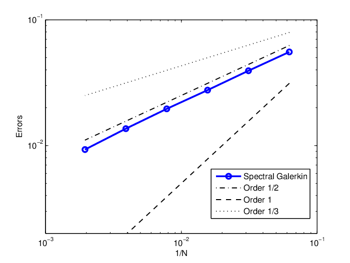
Now let us start with tests on the convergence rates. At first, we consider the spatial convergence rate of the spectral Galerkin method (3). Fig. 2 depicts the spatial approximation errors ‖u⁡(T)−uN​(T)‖L2​(Ω,U)\|u(T)-u^{N}(T)\|_{L^{2}(\Omega,U)} against 1N\frac{1}{N} on a log-log scale, with T=1T=1 and N=2j,j=4,5,…,9N=2^{j},j=4,5,...,9. One can detect that the errors decrease at a slope of order 12\frac{1}{2} as 1N\frac{1}{N} decreases, which is consistent with our previous assertion on the spatial convergence rate. Note that for the temporal discretization we used here the proposed scheme (4.1) at a small time stepsize τe​x​a​c​t=2−7\tau_{exact}=2^{-7}. In addition, Ne​x​a​c​t=214N_{exact}=2^{14} was used to compute the “exact” solution u⁡(T)u(T).

Refer to caption
Fig. 2: Spatial errors for the spectral Galerkin method applied to SWE (100).

We now fix N=100N=100 and compare several time integrators applied to approximate uN​(T),T=1u^{N}(T),\,T=1 using various stepsizes τ=2−j,j=2,3,…,7\tau=2^{-j},j=2,3,...,7. Again, the “exact” solution uN​(1)u^{N}(1) is approximated by the method (4.1) with a very small stepsize τe​x​a​c​t=2−10\tau_{exact}=2^{-10}. In Fig. 3, we present approximation errors caused by different temporal discretizations, including the linear implicit Euler (LIE) scheme [22], the Crank-Nicolson-Maruyama (CNM) scheme [13, 22], the stochastic trigonometric method (STM)[5, 34] and the proposed scheme (4.1). From the left picture of Fig. 3, one can easily observe that the scheme (4.1) performs much better than the other ones. On the one hand, it produces much smaller errors than the other three schemes. On the other hand, computational errors of the scheme (4.1) decrease faster, i.e., with rate 11. To clearly display the convergence rates of the three existing schemes, we change the scales of coordinate axes and hide the computational errors of the scheme (4.1). In the right picture of Fig. 3, one can find that the approximation errors of the linear implicit Euler (LIE) scheme decrease with order 14\frac{1}{4}, the errors of the Crank-Nicolson-Maruyama (CNM) scheme with order 13\frac{1}{3}, and the errors of the stochastic trigonometric method (STM) with order 12\frac{1}{2}. These numerical performances coincide with theoretical findings, see Theorem 5, [22, Theorem 4.12] and [5, Theorem 4.1].

Refer to caption
Refer to caption
Fig. 3: Strong convergence rates in time for various time integrators applied to (3).

For the second example, we look at the nonlinear SWE

{∂2u∂t2=∂2u∂x2+1+u1+u2+W˙,0<t≤1,x∈(0,1),u(0,x)=0,∂u∂t(0,x)=1,x∈(0,1),u(t,0)=u(t,1)=0,t>0.\left\{\begin{array}[]{lll}\frac{\partial^{2}u}{\partial t^{2}}=\frac{\partial^{2}u}{\partial x^{2}}+\frac{1+u}{1+u^{2}}+\dot{W},\quad 0<t\leq 1,\>\>x\in(0,1),\\ u(0,x)=0,\,\frac{\partial u}{\partial t}(0,x)=1,\>x\in(0,1),\\ u(t,0)=u(t,1)=0,\>t>0.\end{array}\right. (101)

Subsequently, we focus on the overall computational efforts of various fully discrete schemes, with the spectral Galerkin discretizations in space. We take the number of realizations of independent random variables needed for approximations as a measure for the computational effort. Recall that the Crank-Nicolson-Maruyama (CNM) scheme and the stochastic trigonometric method (STM) converge with rate 13−ϵ\frac{1}{3}-\epsilon and order 12−ϵ\frac{1}{2}-\epsilon in time, respectively. In space, the spectral Galerkin method converges with order 12−ϵ\frac{1}{2}-\epsilon for arbitrarily small ϵ>0\epsilon>0. In order to balance the errors in space and in time, we set M=N32M=N^{\frac{3}{2}} for CNM scheme and M=NM=N for STM. Similarly, we set M=N12M=N^{\frac{1}{2}} for the schemes (4.1) and (4.1). With these settings, the four schemes all result in an overall approximation error O⁡(N−12+ϵ)O\big(N^{-\frac{1}{2}+\epsilon}\big). The overall approximation errors produced by different schemes are listed in Table 1-3. Note that the “exact” solution is approximated by the spectral Galerkin method in space with Ne​x​a​c​t=212N_{exact}=2^{12} and the STM scheme in time with τe​x​a​c​t=2−12\tau_{exact}=2^{-12}. Again, 100 samples are used for the approximation of the expected values. In Fig. 4 we plot these approximation errors against the number of used random variables. The overall approximation errors of the four schemes all decrease at expected rates, as NN increases. For example, the overall computational errors of the schemes (4.1) and (4.1) both decrease at slope −13-\frac{1}{3}. This is an immediate consequence of our previous setting M=N12M=N^{\frac{1}{2}}. However, the overall errors of the other two methods exhibit decay rates of −15-\frac{1}{5} and −14-\frac{1}{4} as expected. Given a precision ε=0.02\varepsilon=0.02, we are to compare the required computational costs for the above four schemes. One can first detect that the Crank-Nicolson-Maruyama scheme achieves the given precision in the case N=28,M=212N=2^{8},M=2^{12} and thus requires to generate 220=10485762^{20}=1048576 random variables. For the stochastic trigonometric method, 218=2621442^{18}=262144 (N=M=29N=M=2^{9}) random variables are needed to promise the precision. Our proposed schemes (4.1) and (4.1), however, achieve the given precision as N=28,M=24N=2^{8},M=2^{4}, which requires generation of only 2×212=81922\times 2^{12}=8192 random variables. As discussed above, with the same precision, the proposed schemes (4.1) and (4.1) can reduce the number of used random variables greatly and improve the computational efficiency significantly.

Table 1: Computational errors of the Crank-Nicolson-Maruyama scheme with M=N3/2M=N^{3/2}
N=22N=2^{2} N=24N=2^{4} N=26N=2^{6} N=28N=2^{8}
0.13058 0.065411 0.032987 0.016622
Table 2: Computational errors of the stochastic trigonometric method with M=NM=N
N=26N=2^{6} N=27N=2^{7} N=28N=2^{8} N=29N=2^{9}
0.054405 0.037954 0.026312 0.017867
Table 3: Computational errors of the schemes (4.1) and (4.1), with M=N1/2M=N^{1/2}
N=24N=2^{4} N=26N=2^{6} N=28N=2^{8} N= 2102^{10}
Scheme (4.1) 0.055098 0.027929 0.01372 0.0068861
Scheme (4.1) 0.05617 0.028007 0.013708 0.0068762
Refer to caption
Refer to caption
Refer to caption
Refer to caption
Fig. 4: The overall approximation errors against number of used random variables.

6 Conclusion

By incorporating suitable linear functionals of the noise process, two higher order fully discrete schemes have been devised in this work to solve stochastic wave equations with additive space-time white noise. Both theoretical convergence results and numerical experiments show that the proposed schemes can significantly reduce the computational costs, compared with existing methods for the SWE (1). In the present work, we always assume that the drift coefficient satisfies a globally Lipschitz condition, which was commonly used in the literature but excludes many important model equations in applications. In the future, we plan to address this issue and to investigate strong convergence of numerical schemes for nonlinear SWEs in non-globally Lipschitz settings [10, 11]. In addition, another future direction of study is to construct higher order time integrators on the basis of the Taylor expansions of the solution process of SWEs [18].

References

  • [1] E. M. Cabaña, On barrier problems for the vibrating string, Prbab. Theory Rel. Fields, 22 (1972), pp. 13-24.
  • [2] Y. Cao, and L. Yin, Spectral Galerkin method for stochastic wave equations driven by space-time white noise, Commun. Pure Appl. Anal., 6 (2007), pp. 607-617.
  • [3] R. Carmona, and D. Nualart, Random non-linear wave equations: smoothness of the solutions, Probab. Theory Re1. Fields, 79 (1988), pp. 469-508.
  • [4] P. Chow, Stochastic Partial Differential Equations, Chapman &\& Hall/CRC, New York, 2007.
  • [5] D. Cohen, S. Larsson, and M. Sigg, A trigonometric method for the linear stochastic wave equation, SIAM J. Numer. Anal., 51 (2013), pp. 204-222.
  • [6] R.C. Dalang, D. Khoshnevisan, C. Mueller, D. Nualart, and Y. Xiao, A minicourse on stochastic partial differential equations, Lecture Notes in Math. 1962, Springer-Verlag, Berlin, 2009.
  • [7] G. Da Prato, A. Jentzen and M. Roeckner, A mild Itô formula for SPDEs, 2010; available online from http://www.arxiv.org/abs/arXiv:1009.3526.
  • [8] G. Da Prato, and J. Zabczyk, Stochastic Equations in Infinite Dimensions, Encyclopedia Math. Appl. 44, Cambridge University Press, Cambridge, UK, 1992.
  • [9] C. Gardiner, Handbooks of Stochastic Methods for Physics, Chemistry and Natural Sciences, Springer-Verlag, 1983.
  • [10] I. Gyöngy, Lattice approximations for stochastic quasi-linear parabolic partial differential equations driven by space-time white noise I, Potential Anal., 9 (1998), pp. 1-25.
  • [11] I. Gyöngy, Lattice approximations for stochastic quasi-linear parabolic partial differential equations driven by space-time white noise II, Potential Anal., 11 (1999), pp. 1-37.
  • [12] E. Hausenblas, Weak approximation of the stochastic wave equation, J. Comput. Appl. Math., 235 (2010), pp. 33-58.
  • [13] E. Hausenblas, Approximation for semilinear stochastic evolution equations, Potential Anal., 18 (2003), pp. 141-186.
  • [14] A. Jentzen, and P.E. Kloeden, Overcoming the order barrier in the numerical approximation of stochastic partial differential equations with additive space-time noise, Proc. R. Soc. Lond. Ser. A Math. Phys. Eng. Sci., 465 (2009), pp. 649-667.
  • [15] A. Jentzen, and P.E. Kloeden, The numerical approximation of stochastic partial differential equations, Milan J. Math., 77 (2009), pp. 205-244.
  • [16] A. Jentzen and P.E. Kloeden, Taylor Approximations for Stochastic Partial Differential Equations, CBMS-NSF Regional Conf. Ser. in Appl. Math. 83, SIAM, Philadelphia, 2011.
  • [17] A. Jentzen, P.E. Kloeden, and G. Winkel, Efficient simulation of nonlinear parabolic SPDEs with additive noise, Ann. Appl. Probab., 21 (2011), pp. 908-950.
  • [18] A. Jentzen, Higher order pathwise numerical approximations of SPDEs with additive noise, SIAM J Numer. Anal., 49 (2011), pp. 642-667.
  • [19] P.E. Kloeden, and E .Platen, Numerical Solution of Stochastic Differential Equations, Springer, Berlin, 1992.
  • [20] M. Kovács, S. Larsson, and F. Saedpanah, Finite element approximation of the linear stochastic wave equation with additive noise, SIAM J. Numer. Anal., 48 (2010), pp. 408-427.
  • [21] M. Kovács, S. Larsson, and F. Lindgren, Weak Convergence of Finite Element Approximations of Linear Stochastic Evolution Equations with Additive noise, BIT, 52 (2012), pp. 85-108.
  • [22] M. Kovács, S. Larsson, and F. Lindgren, Weak convergence of finite element approximations of linear stochastic evolution equations with additive noise II. Fully discrete schemes, BIT, 53 (2013), pp. 497-525.
  • [23] R. Kruse, Strong and weak approximation of semilinear stochastic evolution equations, PhD thesis, University of Bielefeld, 2012.
  • [24] F. Lindgren, On weak and strong convergence of numerical approximations of stochastic partial differential equations, PhD thesis, Chalmers University of Technology, 2012.
  • [25] A. Martin, S.M. Prigarin, and G. Winkler, Exact and fast numerical algorithms for the stochastic wave equation, Int. J. Comput. Math., 80 (2003), pp. 1535-1541.
  • [26] C. Prévôt, and M. Röckner, A Concise Course on Stochastic Partial Differential Equations, Lecture Notes in Math. 1905, Springer, Berlin, 2007.
  • [27] L. Quer-Sardanyons, and M. Sanz-Solé, Space semi-discretisations for a stochastic wave equation, Potential Anal., 24 (2006), pp. 303-332.
  • [28] H. Schurz, Analysis and discretization of semi-linear stochastic wave equations with cubic nonlinearity and additive space-time noise, Discrete Contin. Dyn. Syst. Ser. S, 1 (2008), pp. 353-363.
  • [29] V. Thomée, Galerkin Finite Element Methods for Parabolic Problems, Springer Verlag, 2006.
  • [30] H. Triebel, Interpolation Theory, Function Spaces, Differential Operators, North-Holland Publishing Co., Amsterdam, 1978.
  • [31] J.B. Walsh, An Introduction to Stochastic Partial Differential Equations, Lecture Notes in Math. 1180, Springer-Verlag, 1986.
  • [32] J.B. Walsh, On numerical solutions of the stochastic wave equation, Illinois J. Math., 50 (2006), pp. 991-1018.
  • [33] X. Wang, and S. Gan, A Runge-Kutta type scheme for nonlinear stochastic partial differential equations with multiplicative trace class noise, Numer. Algor., 62 (2013), pp. 193-223.
  • [34] X. Wang, An exponential integrator scheme for time discretization of nonlinear stochastic wave equation, 2013; available online from http://www.arxiv.org/abs/arXiv:1312.5185.