Interplay between Kondo and Majorana interactions in quantum dots

In order to identify the IR fixed point the systems flows to, we study the RG flow of the boundary couplings. The minimal system of RG equations involves four couplings $h(0)=-|\lambda|^{2}\xi_{-}$, $J_{1}(0)=\lambda|t|\xi_{-}$, $J_{2}(0)=\lambda|t|\xi_{+}$ and $J_{3}(0)=|t|^{2}\xi_{+}$, see Eq. (4). In the weak-coupling limit $t\rightarrow 0$, we impose open boundary conditions for lead electrons, and then identify a leading relevant operator that drives the system away from the unstable fixed point. Henceforth, we assume that the normal lead has spin-SU(2) symmetry, i.e. $K_{\sigma}=1$. Then, the RG equations up to quadratic order in couplings are given by

with $l$ being the logarithmic length scale. One can see that $h$ is relevant and tends to polarize the spin on the dot. The couplings $J_{1}$ and $J_{2}$ are relevant when $K_{\rho}>1/3$, whereas the Kondo coupling $J_{3}$ is marginal. The competition between Majorana and Kondo interactions is reflected in the RG flow of $J_{2}(l)$, see second order correction proportional to $J_{3}J_{2}$. However, in the weak coupling limit, we have $J_{3}/\pi v_{\sigma}\ll 1$ and the Majorana coupling dominates. Thus, we conjecture that the strong coupling fixed point is governed by the Majorana rather than the Kondo interaction. At the length scales $l^{*}$ where the Zeeman coupling becomes dominant (i.e. $h(l^{*})\gg J_{2}(l^{*})$), the spin on the QD is completely polarized along the $\hat{z}$-axis, and, thus, the IR fixed point corresponds to Andreev boundary condition (ABC) for spin-up electrons and normal boundary condition (NBC) for spin-down electrons, a situation which we denote as $A\otimes N$ fixed point (i.e. $\psi_{R\uparrow}^{\dagger}(0)=\psi_{L\uparrow}(0)$ and $\psi_{R\downarrow}(0)=\psi_{L\downarrow}(0)$). The tunneling conductance through such a system is quantized in units of $2e^{2}/h$, similar to a TSC/Luttinger liquid (LL) junctions [73, 74]. One can also understand the temperature and voltage corrections to the tunneling conductance using the previous results for TSC/LL junctions [75]. From the structure of the lead-Majorana couplings in Eq. (4), one can immediately notice that the broadening of the zero-bias conductance peak gets renormalized by the charging energy $U$. The decrease of the resonance width can be understood as a competition between the charging energy $U$ suppressing charge fluctuations on the dot and the coupling to the Majorana mode $\gamma_{1}$ favoring charge fluctuations.

The above analysis relies on perturbative RG equations which are, strictly speaking, not valid at strong coupling. Therefore, in order to access the strong coupling fixed point, we perform numerical simulations for our model. If the predictions based on the aforementioned weak-coupling analysis hold in the strong coupling limit, the system would flow to Andreev and normal boundary conditions for spin-up and spin-down, respectively. The difference in the boundary conditions for spin-up and spin-down electrons should be visible in various static correlation functions such as, for example, superconducting triplet correlation function defined as

One can show that at the $A\otimes N$ fixed point, $T_{\sigma}(x)$ decays as $T_{\sigma}(x)\propto|x|^{d_{\sigma}}$ where $d_{\uparrow}=-1/2(K_{\rho}^{-1}+1)$ and $d_{\downarrow}=-3/2(K_{\rho}^{-1}+1)$. Within a bosonization perspective, this can be understood as follows: Andreev boundary conditions for spin-up electrons lead to the suppression of $\theta_{\uparrow}$ fluctuations at the boundary, hence the decay of spin-triplet correlations is slower than in the bulk where $T_{\sigma}(x,x^{\prime})\propto|x-x^{\prime}|^{-(K_{\rho}^{-1}+1)}$ [76]. On the contrary, $\theta_{\downarrow}$ fluctuates strongly at the boundary and, therefore, the correlation function $T_{\downarrow}(x)$ decays much faster than in the bulk. This drastic difference in the spin-up/down correlation function should be contrasted with the one at $\lambda=0$, where the system flows to the Kondo fixed point with $d_{\uparrow}=d_{\downarrow}$.

To corroborate this picture, we perform simulations using the density-matrix renormalization group method [79, 80, 81, 82]. This method has previously been applied with enormous success to many one-dimensional models, including models for the Kondo effect [83, 84, 85, 86, 87, 88]. We perform simulations directly for the Hamiltonian (4), with a real-space discretization with constant hopping for the normal lead, see Eq. (3). Such a setup allows easy access to real-space correlation functions. DMRG simulations can be systematically refined by increasing a parameter of the simulation, the so-called matrix size $M$. We perform simulations with matrix sizes up to $M=800$, ensuring accurate results also for the gapless lead. We use system sizes with an odd number of sites in the lead to allow for the ground state of the entire system to be an SU(2) singlet. Our system sizes are up to 127 sites in the lead. For the purpose of this paper, we fix the lead to half filling and set $U_{b}=0$ to avoid any CDW or pairing instabilities in the lead.

Numerical results for the superconducting triplet correlation function, defined in Eq. (6), are shown in Fig. 2. As one can see from the figure, the correlation function $T_{\sigma}(x)$ for spin-up and spin-down electrons decays with different exponents $d_{\uparrow}$ and $d_{\downarrow}$. From the scaling analysis with the system size $L$, shown in the inset of the figure, we extract $d_{\uparrow}\approx-1$ and $d_{\downarrow}\approx-3$, which is in excellent agreement with the predictions for $A\otimes N$ boundary conditions, see the discussion above. Thus, we confirm that the strong coupling fixed point is indeed controlled by the Majorana interaction rather than the Kondo interaction, which is one of the main results of the paper.

We now emphasize the difference in transport properties for nanostructures involving topological and non-topological superconductors. In the absence of the Majorana coupling, one needs to take into account Andreev scattering at the junction, $H\propto J_{AB}\psi_{\sigma}(0)\psi_{-\sigma}(0)+h.c.$. Indeed, in the free-fermion limit ($K=1$) both Andreev and Kondo boundary couplings are marginal and compete with each other. Thus, low energy transport properties of the junction involving a non-topological superconductor (NTSC) depend on the microscopic details, i.e. the ratio of $J_{3}/J_{AB}$, see also discussion in Sec.III.4.

In this section we focus on the particle-hole symmetric point corresponding to a vanishing Zeeman term, i.e. $\xi_{-}=0$. The resulting boundary Hamiltonian is given by

where $\eta_{a}(0)$ are Majorana operators at $x=0$ defined as $\eta_{x}=\psi_{\downarrow}(0)+\psi^{\dagger}_{\downarrow}(0)$, $\eta_{y}=i(\psi^{\dagger}_{\downarrow}(0)-\psi_{\downarrow}(0))$ and $\eta_{z}=\psi_{\uparrow}(0)+\psi^{\dagger}_{\uparrow}(0)$. One can see that $J_{2}$ flows to strong coupling, and, as a result, the system forms an entangled state involving fermion parity shared between the $\gamma_{1}$ and $\eta_{a}(0)$ modes and the impurity spin. However, the nature of the boundary conditions for fermions at $x=0$ is quite non-trivial since the spin on the dot is strongly fluctuating. This can be understood from an emergent symmetry of the system. Indeed, at this special point the effective Hamiltonian is invariant under the following anti-unitary symmetry:

Here $K$ is the complex conjugation and $\mathcal{C}$ is the charge conjugation, under which $d_{\sigma}\rightarrow d_{\sigma}^{\dagger}$ and $\psi_{\sigma}\rightarrow\psi_{\sigma}^{\dagger}$. One can show that $[\tilde{\mathcal{T}},H_{b}+H_{\text{NL}}]=0$. When acting on the QD impurity spin, $\tilde{\mathcal{T}}$ is similar to the time-reversal symmetry $\tilde{\mathcal{T}}{\mathbf{S}}\tilde{\mathcal{T}}^{-1}=-{\mathbf{S}}$ which implies that $\langle{\mathbf{S}}\rangle=0$. Away from the particle-hole symmetric point, both terms proportional to $\xi_{-}$ explicitly break $\tilde{\mathcal{T}}$-symmetry, and induce a polarization of the impurity spin along $z$-axis.

Some insight regarding the IR fixed point in this case can be obtained when leads are non-interacting and $J_{3}=0$. By introducing Majorana fermion operators $\Gamma_{a}=2\gamma_{1}S_{a}$, the problem can be mapped to a fermion bilinear Hamiltonian which admits an exact solution. One can show that the operators $\Gamma_{a}$ satisfy canonical commutation relations and anticommute with all other fermion operators, i.e. $\left\{\Gamma_{a},c_{\sigma}\right\}=0$. We now consider the Hilbert space these matrices act upon. The Hilbert space of the original problem is given by a tensor product of the topological superconductor and the quantum dot, which is described by $4\times 4$ matrices forming a Clifford algebra. On the other hand, after the mapping we also have a Clifford algebra $\{\gamma_{2},\Gamma_{x},\Gamma_{y},\Gamma_{z}\}$. The uniqueness of the Clifford algebra up to a unitary transformation ensures that the matrix representations of $\gamma_{1}S_{a}$ and $\Gamma_{a}$ are equivalent. Using this mapping, one can set up a standard transport calculation [89]. We first compute the unitary scattering matrix $S(E)$ defined as

where the matrix $W$ describes the coupling of Majorana modes $(\Gamma_{x},\Gamma_{y},\Gamma_{z}$) to the lead degrees of freedom:

Here, the propagating electron and hole modes in the normal lead are described in the basis $(\psi_{\uparrow},\psi_{\downarrow},\psi^{\dagger}_{\uparrow},\psi^{\dagger}_{\downarrow})$. Using the particle-hole components of the scattering matrix $P_{he}(E)$, one finds that the dc current through the system is given by

where $A(E)$ is the probability of Andreev reflection, $f(E)$ is the Fermi function and $V$ is an applied bias voltage. The tunneling conductance through the junction $G=dI/dV$ at zero temperature reads

Here the broadening width due to the coupling to Majorana modes $\Gamma_{i}$ is $W_{i}=\pi J_{i}^{2}\nu_{F}$ with $i=x,y,z$ and $\nu_{F}$ being density of states in the lead. Since $J_{x}=J_{y}=J_{z}=J_{2}$ (see Eq.(7)), the second term in the above equation vanishes, and we find that the low-bias conductance is equal to $G(0)=2e^{2}/h$ at zero temperature, similar to the NM-MBS case [73, 74]. The quantization of the conductance in units of $e^{2}/h$ corresponds to Andreev boundary conditions for spin-up electrons and normal boundary conditions for the spin-down electrons. Indeed, the spin-down electrons are coupled to two Majoranas, $\Gamma_{x}$ and $\Gamma_{y}$, which effectively annihilate each other, i.e. the contribution to the conductance from $\Gamma_{x}$ and $\Gamma_{y}$ is zero. Using Eqs. (13) and (15), one finds that the temperature and voltage dependence of the conductance $G(V,T)$ at the particle-hole symmetric point is similar to that of NM-MBS junction [75] with the width being determined by $W$. We note here that our results on the conductance at the particle-hole symmetric point are different from those of Ref. 66, who find that the zero-bias tunneling conductance has a temperature dependence which is distinct from that of the simpler NM-MBS tunnel junction ¹¹ 1 We notice that Ref. 66 also derived RG equations for the same microscopic Hamiltonian at the particle-hole symmetric point for the non-interacting lead ($K_{\rho}=K_{\sigma}=1$), but missed the tree-level scaling term for the flow of $J_{2}$. The RG equations in Ref. 66 were obtained using field-theoretic method involving the scale invariance of the conductance. The disagreement with our momentum-shell Wilsonian RG approach originates from the fact that the coupling $J_{2}$ has a non-zero engineering (naive) dimension and should be rescaled to be dimensionless before computing the RG flow using the Callan-Symanzik equation. This discrepancy, however, leads to an incorrect identification of the strong coupling fixed point and invalidates the conclusions of Ref. 66..

Further insight about the strong coupling fixed point can be obtained by studying the dynamics of the impurity spin. Consider, for example, the dynamical spin-spin correlation function $\langle S_{z}(t)S_{z}(0)\rangle$. The impurity spin operator can be written in terms of Majorana operators $\Gamma_{a}$: $S_{a}=-2i\varepsilon_{abc}S_{b}S_{c}=-\frac{i}{2}\varepsilon_{abc}\Gamma_{b}\Gamma_{c}$. Then, the correlation function $\langle S_{z}(t)S_{z}(0)\rangle$ can be written as

The correlation function $G(t)=\langle\Gamma_{a}(t)\Gamma_{a}(0)\rangle$ can be easily obtained by taking the Fourier transform of

where $a=x,y,z$. Since $J_{x}=J_{y}=J_{z}$, we define $W\equiv W_{a}$. In the long-time limit, spin-spin correlation function reads

Clearly, the impurity spin operator acquires a non-trivial scaling dimension equal to one at the strong coupling fixed point, and, thus, Kondo coupling $J_{3}$ becomes an irrelevant perturbation in the RG sense. We confirm our results using DMRG calculations and show that the system flows to $A\otimes N$ boundary conditions when $J_{3}\neq 0$, see Fig. 3. One can see that for $\lambda=0$, the decay of triplet correlation functions is described by the same exponent for spin-up and spin-down electrons $d_{\uparrow}=d_{\downarrow}$. However, as soon as $\lambda\neq 0$, the exponents become different and eventually saturate at $d_{\uparrow}\approx-1$ and $d_{\downarrow}\approx-3$ for non-interacting leads. These numerical results corroborate our conjecture that in the presence of particle-hole symmetry the strong coupling fixed point is described by a new fixed point dictated by $J_{2}$ coupling. This fixed point corresponds to a situation where the spin on the dot is strongly entangled with the combined fermion parity of the topological superconductor and the normal lead.

Another interesting feature of the above fixed point is the dependence of the polarization of the impurity spin on the position of the energy level $\varepsilon$ on the dot. At the particle-hole symmetric point $\varepsilon=\varepsilon_{0}=-U/2$, the impurity spin is strongly fluctuating, i.e. $\langle S_{z}\rangle=0$. If the gate voltage is detuned by $V_{g}$, such that $\varepsilon=\varepsilon_{0}+V_{g}$, the spin shows a non-trivial behavior that allows us to distinguish between Majorana and Kondo physics. As the Kondo coupling does not break the $\tilde{\mathcal{T}}$-symmetry, the impurity spin has an expectation value $\langle{\mathbf{S}}\rangle=0$ for all values of $V_{g}$ in the absence of a coupling to the Majorana mode, $\lambda=0$. If, on the other hand, the coupling to the Majorana mode is present, $\lambda\neq 0$, the spin polarizes along the $\hat{z}$-axis for $V_{g}\neq 0$, see discussion after Eq. (8). The perturbation Hamiltonian proportional to the detuning away from the particle-hole symmetric point $V_{g}$ is given by

Using linear response theory, one can now compute the spin susceptibility $\partial\langle S_{z}\rangle/\partial V_{g}\big|_{V_{g}=0}$. Consider the imaginary-time dynamical spin response function:

Using the relation $S_{z}=-\frac{i}{2}\Gamma_{x}\Gamma_{y},\gamma_{1}=-i\Gamma_{x}\Gamma_{y}\Gamma_{z}$, one obtains

where the Green’s function $G_{xy}(\tau)=-\langle T_{\tau}f(\tau)f^{\dagger}(0)\rangle$ with $f=\frac{1}{2}(\Gamma_{x}+i\Gamma_{y})$. Using the equations of motion, one can find $G_{xy}(i\omega)=(i\omega+iW\sgn\omega)^{-1}$. After some manipulations, we obtain the static spin susceptibility $\partial\langle S_{z}\rangle/\partial V_{g}\big|_{V_{g}=0}\equiv\chi(\omega\rightarrow 0)$,

with $\Lambda$ being the UV cutoff corresponding to the bandwidth in the lead and $\xi_{+}=\frac{4}{U}$. Close to the particle-hole symmetric point, the susceptibility $\partial\langle S_{z}\rangle/\partial V_{g}$ has a non-trivial dependence on the tunneling rates $\lambda$ and $t$. This dependence is very distinct from the Kondo case suggesting that studies of impurity spin fluctuations in TSC-QD-NL structures might be used to help identifying Majorana zero-energy modes.

To numerically confirm this behavior, we resort to DMRG simulations of the system. We simulate systems up to $L=64$ sites described by Hamiltonian (4), where we set $U=8$ and $t=1$. For our simulations, we use $M=400$ states and we measure $\langle S_{z}\rangle$ on the impurity. We slightly detune the chemical potential on the quantum dot from the particle-hole symmetric point and perform simulations in the range $V_{g}\in[-0.05,0.05]$, allowing us to numerically extract the derivative $\partial\langle S_{z}\rangle/\partial V_{g}$. To gain additional insight into the crossover between Kondo- and Majorana-dominated physics, we modify the Hamiltonian (4) by multiplying the Kondo coupling term by an additional factor $K$ to either suppress or enhance the Kondo energy scale. Our results are shown in Fig. 4. We find that for intermediate values of $\lambda$ and in particular the physical limit $K=1$, the susceptibility can be well fit by a $\log\lambda^{2}$, as suggested by (22). If $\lambda\sim 1$ or $\lambda$ is much smaller than the level spacing in the lead, finite-size effects become significant and our previous calculation in the thermodynamic limit is no longer applicable. We have checked that a modified theory on finite-size lattice systems reproduces the numerical data very well. We observe that enhancing the Kondo coupling suppresses the spin susceptibility. This is easily understood by considering that in the Kondo-dominated strong-coupling fixed point, i.e. for $\lambda\ll t$, the impurity spin forms a singlet with lead electrons, i.e. $\langle S\rangle\rightarrow 0$ and, thus, the susceptibility vanishes.

The results discussed in the previous section are valid close to the particle-hole symmetric point. We now develop a theory away from this point in the large-$U$ limit. In this case one can use a slave boson approximation [91, 92] proven to successfully capture the strong correlation effect in the Anderson impurity models, see, e.g., Ref. 93. In order to take into account the interplay between the Kondo correlation and the Majorana coupling, we go back to the initial Anderson-type model of the TSC-QD-NL junction and project out the doubly occupied state using a mean-field slave boson approximation (MFSBA). A similar study was carried out in Ref. 66 but, as explained below, the non-trivial mean-field solution corresponding to the Majorana-dominated regime, which is the main result of our paper, was not treated there. To make this section self-contained, we briefly review the slave boson approach and discuss mean field solutions in different parameter regime. Technical details are presented in the Appendix C.

We begin by writing the Anderson Hamiltonian for the TSC-QD-NL junction:

where $\psi_{k\sigma}$ are fermion annihilation operators in the normal lead, and $\delta$ is the ground state degeneracy splitting in the TSC due to finite size effects. In the infinite-$U$ limit, double occupancy of the QD is suppressed. To this end we introduce new operators $d_{\sigma}\rightarrow f_{\sigma}b^{\dagger}$ and $d^{\dagger}_{\sigma}\rightarrow f^{\dagger}_{\sigma}b$ where $b$ and $f_{\sigma}$ represent unoccupied and singly-occupied states, respectively. Double occupancy is excluded by introducing the constraint $b^{\dagger}b+\sum_{\sigma}f_{\sigma}^{\dagger}f_{\sigma}=1$. Thus, the effective action of the system reads

where the last term enforces the constraint on the Hilbert space. We now make a mean-field approximation and replace boson operators by their expectation value $\langle b\rangle=\langle b^{\dagger}\rangle=b$, which together with the Lagrange multiplier $\eta$ are going to be determined self-consistently by minimizing the action $S_{\rm sb}$:

The calculation of the above correlation functions is presented in the Appendix C. Here we highlight our main results.

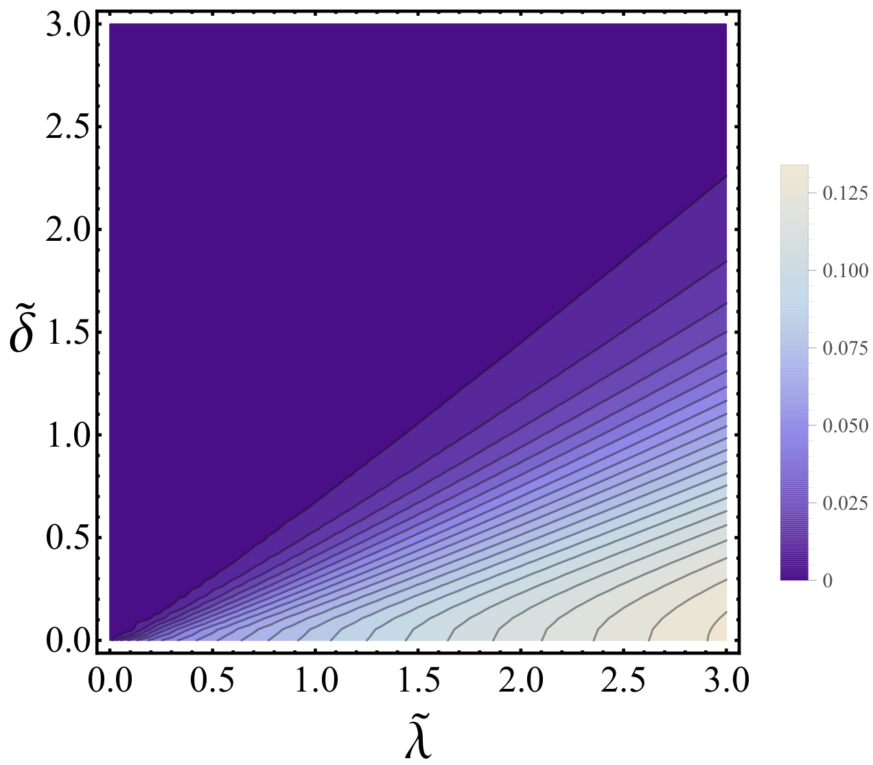
The general solution can be obtained numerically as well as, in some cases, analytically. We first consider the case of no splitting $\delta=0$. In the single-occupancy limit where $\varepsilon<0$ and $|\varepsilon|\gg\lambda,|t|$, the probability of a QD being empty $b^{2}$ is small. Thus, one can solve the self-consistency equations assuming $b\rightarrow 0$. From the first equation above, we find that $|\varepsilon+\eta|\sim\Gamma b^{4}$ with $\Gamma=\pi|t|^{2}\nu_{F}$ being the lead-induced broadening in the dot. Using the expression for $\eta$ and evaluating the integrals in the second equation, one finds

Here we kept only leading terms in the expansion in small $b$; $\Lambda$ is a UV cutoff corresponding to the bandwidth in the lead. When $\lambda=0$, we recover the solution for the Kondo model

and $\Gamma b^{2}=\Lambda e^{-\frac{\pi|\varepsilon|}{2\Gamma}}\equiv T_{K}$ corresponds to the Kondo temperature $T_{K}$. When $\lambda$ is large, the second term in Eq. (28) is more important since it is more divergent. Thus, an approximate solution reads

This is a new mean-field solution of the self-consistency equations which was not considered in Ref. 66. Once again, we see that the Majorana coupling is a more relevant perturbation than the Kondo coupling and, thus, determines the low energy properties of the system. The crossover between the two regimes can be determined by matching the two solutions for $b$:

Thus, the Majorana-dominated regime corresponds to $\lambda\gg\lambda_{c}$ with the value of $b$ determined by the Majorana coupling whereas $\lambda\ll\lambda_{c}$ corresponds to the Kondo-dominated regime.

We will now discuss finite size effects in the nanowire by assuming that Majorana degeneracy splitting $\delta$ is non-zero. In this case, we find solutions of Eqs. (27) numerically. A plot of $b$ as a function of the rescaled parameters $\tilde{\delta}=\delta/\Gamma,\tilde{\lambda}=\lambda/\Gamma$ is shown in Fig. 5. One can see that when $\delta$ is large, the value of $b$ closely tracks Eq. (29). As $\delta$ is increased there is a crossover between the Majorana-dominated regime and the Kondo-dominated regime. As expected, the splitting energy $\delta$ reduces the parameter space corresponding to the Majorana-dominated regime.

Having solved the mean-field equations for $b$ and $\eta$, we can now compute experimentally observable quantities. In this section, we study the differential tunneling conductance, having in mind a setup similar to that of Ref. 19, see Fig. 1. At the qualitative level one can already see that, once the parameters $\eta$ and $b$ are determined within the MFSBA, the dynamics of spin-up and -down electrons decouple. Spin-down electrons do not contribute to Andreev reflection since they are not coupled to the Majorana mode $\gamma_{1}$.²² 2 Here we neglect Andreev scattering terms proportional to $d_{\uparrow}d_{\downarrow}+h.c.$ which are suppressed by the large superconducting gap. Thus, the mean-field results are consistent with the boundary conditions $A_{\uparrow}\otimes N_{\downarrow}$. Using the scattering matrix formalism outlined in Sec.III.2, see Eq.(9), one can find the probability of Andreev reflection:

where $\tilde{\varepsilon}=\varepsilon+\eta$. The differential tunneling conductance can be obtained with the help of Eq. (13), and is given by $G(V)=\frac{2e^{2}}{h}A(eV)$ at zero temperature. One can see that the functional dependence $G(V)$ is different from the Lorentzian form characteristic to the simpler TPSC-NL structures and has a much richer structure. At zero splitting $\delta=0$, the conductance is still quantized at zero bias $G(0)=2e^{2}/h$ but the broadening of the resonance is a non-trivial function of various parameters:

The value of $b$ in Majorana- and Kondo-dominated regimes is $b\approx\lambda/\sqrt{8}|\varepsilon|$ and $b\approx\sqrt{T_{K}/\Gamma}$, respectively. At small bias $V\rightarrow 0$, one can estimate the effective width of the resonance $\Gamma_{\rm eff}$ to be

These results can be understood as follows. In the Majorana-dominated regime, the physics of the QD is determined by the Majorana strong coupling fixed point. Therefore, the width of the resonance is proportional to $t^{2}\lambda^{2}\nu_{F}/|\varepsilon|^{2}\sim W$. This is consistent with the results at the particle-hole symmetric point, see Sec. III.2. The Kondo-dominated regime corresponds to the small-$\lambda$ limit, where the Majorana mode $\gamma_{1}$ is localized in the TSC and is only weakly coupled to the QD. The effective width of the zero-bias peak is determined by the smaller of the two rates $T_{K}$ and $\lambda^{2}/\Gamma$, and therefore is much sharper than in the Majorana-dominated regime where the width of the resonance is suppressed only as a power law in $|\varepsilon|$. Another interesting feature in the tunneling conductance is the appearance of the sidebands as shown in Fig. 6(a). These sidebands originate from the splitting of the Kondo resonance by the induced Zeeman term, Eq. (4). In our model coupling to the TSC breaks the $U(1)$ charge conservation as well as the time-reversal symmetry. Both these effects lead to the suppression of the Kondo effect. In the Majorana-dominated regime finite-bias resonances appear at $eV=\pm\lambda b\sim\lambda^{2}/|\varepsilon|$ ³³ 3 Note that we have neglected the effect of an external magnetic field $B$ here assuming that the $g$-factor in the QD is small. If Zeeman splitting due to an external $B$ is larger than the exchange-induced one then the position of the sidebands will be determined by the Zeeman term. We believe this is the case in the recent Majorana experiments [19].; the width of these resonances is of the order of $W$.

We note that the aforementioned dependence on $\lambda$ is very different from the one in the s-wave SC-QD-NL junction [63, 68, 69] where Majorana interaction is absent ($\lambda=0$). This can be understood most easily in the limit of a large superconducting gap $\Delta\rightarrow\infty$ (i.e. $\Delta\gg\Gamma_{S},\,\Gamma,\,T_{K}$), where one can integrate out SC degrees of freedom. In the low energy approximation, the effect of an s-wave superconductor can be represented as Andreev scattering term $H_{P}=\Gamma_{S}d_{\uparrow}^{\dagger}d_{\downarrow}^{\dagger}+h.c.$. This term breaks $U(1)$ symmetry and competes with the Kondo singlet state. It has been shown that the Abrikosov-Suhl resonance in the tunneling conductance, present at small $\Gamma_{S}\ll\Gamma$, gets gradually suppressed with the increase of the coupling to a superconductor, see Refs. [96, 97, 98] for details. This behaviour should be contrasted with $G(V)$ shown in Fig.6 where the zero-bias peak becomes more pronounced with increasing of the coupling to TSC. We note, however, that in the non-perturbative regime (i.e. $\Delta\sim\Gamma_{S},\,\Gamma,\,T_{K}$) the situation is more complicated due to the possible appearance of the Shiba-like bound states induced by an unpaired electron spin in the QD [99]. If Shiba levels are close to the Fermi energy, one would expect to observe an enhancement in the subgap tunneling conductance. Thus, it is important to control the coupling and keep it small, $\Gamma_{S}\ll\Delta$, so that the contribution of the Shiba states to the zero-bias tunneling conductance is suppressed. Overall, we find that there is a wide parameter regime $T_{K}\ll\Gamma_{S}/\lambda\ll\Delta$ where the dependence of the zero-bias peak on the coupling to the superconductor is very different for topological and non-topological states allowing one to distinguish between Kondo and Majorana physics.

We now discuss effect of the splitting energy $\delta\neq 0$ due to a finite size of the TSC. Analytical results are not particularly illuminating in this case, and we present numerical solution instead. The plots of the tunneling conductance as a function of various parameters are shown in Fig.6b-d. Overall, many qualitative features can be understood as a convolution of the local density of states in the TSC and QD. At small $\lambda$ the splitting energy leads to the emergence of the two sharp peaks at energies $\pm\delta$, see Fig.6b, the width of these peaks becomes larger with the increase of $\lambda$. Eventually, when $\lambda^{2}/|\varepsilon|\gg\delta$, the shape of the conductance $G(V)$ changes qualitatively: two sideband peaks located at $eV\sim\lambda^{2}/|\varepsilon|$ emerge. In this limit, the position of the peaks and their width are weakly dependent on $\delta$, compare Fig.6a and b. The splitting, however, strongly affects the zero-bias feature and eliminates the zero-bias peaks entirely.

So far we have considered zero temperature limit $T=0$. Using Eq. (13) and (32), we now calculate the temperature dependence of the differential tunneling conductance. The plot of $G(V,T)$ is shown in Fig. 7. The triple peak structure in Fig. 7a gets smeared by the temperature, and one might have to go to very small temperatures in order to observe this feature, especially in the small $\lambda$-limit (i.e. Kondo-dominated regime). In the case of a finite splitting $\delta\neq 0$, the width of the peak becomes more narrow. As a result, tunneling conductance is suppressed even faster by thermal fluctuations, see Fig.7c.

References

- [1] E. S. Reich, “A solid case for majorana fermions,” Nature (London) 483, 132 (2012).
- [2] P. W. Brouwer, “Enter the Majorana Fermion,” Science 336, 989 (2012).
- [3] F. Wilczek, “Quantum physics: Majorana modes materialize,” Nature (London) 486, 195 (2012).
- [4] G. Moore and N. Read, “Nonabelions in the fractional quantum hall effect,” Nucl. Phys. B 360, 362 (1991).
- [5] C. Nayak and F. Wilczek, “2n-quasihole states realize 2n-1-dimensional spinor braiding statistics in paired quantum Hall states,” Nucl. Phys. B 479, 529 (1996).
- [6] N. Read and Dmitry Green, “Paired states of fermions in two dimensions with breaking of parity and time-reversal symmetries and the fractional quantum hall effect,” Phys. Rev. B 61, 10267 (2000).
- [7] D. A. Ivanov, “Non-abelian statistics of half-quantum vortices in -wave superconductors,” Phys. Rev. Lett. 86, 268 (2001).
- [8] Chetan Nayak, Steven H. Simon, Ady Stern, Michael Freedman, and Sankar Das Sarma, “Non-abelian anyons and topological quantum computation,” Rev. Mod. Phys. 80, 1083 (2008).
- [9] Liang Fu and C. L. Kane, “Superconducting proximity effect and majorana fermions at the surface of a topological insulator,” Phys. Rev. Lett. 100, 096407 (2008).
- [10] Liang Fu and C. L. Kane, “Josephson current and noise at a superconductor/quantum-spin-hall-insulator/superconductor junction,” Phys. Rev. B 79, 161408(R) (2009).
- [11] Jay D. Sau, Roman M. Lutchyn, Sumanta Tewari, and S. Das Sarma, “Generic new platform for topological quantum computation using semiconductor heterostructures,” Phys. Rev. Lett. 104, 040502 (2010a).
- [12] Jason Alicea, “Majorana fermions in a tunable semiconductor device,” Phys. Rev. B 81, 125318 (2010).
- [13] Roman M. Lutchyn, Jay D. Sau, and S. Das Sarma, “Majorana fermions and a topological phase transition in semiconductor-superconductor heterostructures,” Phys. Rev. Lett. 105, 077001 (2010).
- [14] Yuval Oreg, Gil Refael, and Felix von Oppen, “Helical liquids and majorana bound states in quantum wires,” Phys. Rev. Lett. 105, 177002 (2010).
- [15] A. Cook and M. Franz, “Majorana fermions in a topological-insulator nanowire proximity-coupled to an s-wave superconductor,” Phys. Rev. B 84, 201105 (2011).
- [16] J. D. Sau and S. D. Sarma, “Realizing a robust practical Majorana chain in a quantum-dot-superconductor linear array,” Nat. Commun. 3 (2012), 10.1038/ncomms1966.
- [17] S. Nadj-Perge, I. K. Drozdov, B. A. Bernevig, and A. Yazdani, “Majorana fermions in chains of magnetic atoms on a superconductor,” Phys. Rev. B 88, 020407(R) (2013).
- [18] A. Yu Kitaev, “Unpaired majorana fermions in quantum wires,” Physics-Uspekhi 44, 131 (2001).
- [19] V. Mourik, K. Zuo, S. M. Frolov, S. R. Plissard, E. P. A. M. Bakkers, and L. P. Kouwenhoven, “Signatures of Majorana Fermions in Hybrid Superconductor-Semiconductor Nanowire Devices,” Science 336, 1003– (2012).
- [20] K. Sengupta, Igor Žutić, Hyok-Jon Kwon, Victor M. Yakovenko, and S. Das Sarma, “Midgap edge states and pairing symmetry of quasi-one-dimensional organic superconductors,” Phys. Rev. B 63, 144531 (2001).
- [21] C. J. Bolech and Eugene Demler, “Observing majorana bound states in -wave superconductors using noise measurements in tunneling experiments,” Phys. Rev. Lett. 98, 237002 (2007).
- [22] Johan Nilsson, A. R. Akhmerov, and C. W. J. Beenakker, “Splitting of a cooper pair by a pair of majorana bound states,” Phys. Rev. Lett. 101, 120403 (2008a).
- [23] K. T. Law, Patrick A. Lee, and T. K. Ng, “Majorana fermion induced resonant andreev reflection,” Phys. Rev. Lett. 103, 237001 (2009).
- [24] Jay D. Sau, Sumanta Tewari, Roman M. Lutchyn, Tudor D. Stanescu, and S. Das Sarma, “Non-abelian quantum order in spin-orbit-coupled semiconductors: Search for topological majorana particles in solid-state systems,” Phys. Rev. B 82, 214509 (2010b).
- [25] Karsten Flensberg, “Tunneling characteristics of a chain of majorana bound states,” Phys. Rev. B 82, 180516 (2010).
- [26] Anatoly Golub and Baruch Horovitz, “Shot noise in a majorana fermion chain,” Phys. Rev. B 83, 153415 (2011).
- [27] M Wimmer, A R Akhmerov, J P Dahlhaus, and C W J Beenakker, “Quantum point contact as a probe of a topological superconductor,” New J. Phys. 13, 053016 (2011).
- [28] R. M. Lutchyn, T. D. Stanescu, and S. Das Sarma, “Search for Majorana Fermions in Multiband Semiconducting Nanowires,” Phys. Rev. Lett. 106, 127001 (2011).
- [29] Tudor D. Stanescu, Roman M. Lutchyn, and S. Das Sarma, “Majorana fermions in semiconductor nanowires,” Phys. Rev. B 84, 144522 (2011).
- [30] Chunlei Qu, Yongping Zhang, Li Mao, and Chuanwei Zhang, “Signature of majorana fermions in charge transport in semiconductor nanowires,” arXiv:1109.4108 (2011).
- [31] Jason Alicea, Yuval Oreg, Gil Refael, Felix von Oppen, and Matthew P. A. Fisher, “Non-abelian statistics and topological quantum information processing in 1d wire networks,” Nature Phys. 7, 412–417 (2011).
- [32] Jay D. Sau, Sumanta Tewari, and S. Das Sarma, “Universal quantum computation in a semiconductor quantum wire network,” Phys. Rev. A 82, 052322 (2010c).
- [33] David J. Clarke, Jay D. Sau, and Sumanta Tewari, “Majorana fermion exchange in quasi-one-dimensional networks,” Phys. Rev. B 84, 035120 (2011).
- [34] Parsa Bonderson and Roman M. Lutchyn, “Topological quantum buses: Coherent quantum information transfer between topological and conventional qubits,” Phys. Rev. Lett. 106, 130505 (2011).
- [35] B. van Heck, A. R. Akhmerov, F. Hassler, M. Burrello, and C. W. J. Beenakker, “Coulomb-assisted braiding of majorana fermions in a josephson junction array,” New J. Phys. 14, 035019 (2012).
- [36] A. Kitaev, “Fault-tolerant quantum computation by anyons,” Ann. Phys. 303, 2 (2002).
- [37] Michael H. Freedman, “P/np, and the quantum field computer,” Proc. Natl. Acad. Sci. 95, 98 (1998).
- [38] L. P. Rokhinson, Xinyu Liu, and Jacek K. Furdyna, “Observation of the fractional ac josephson effect: the signature of majorana particles,” Nature Phys. 8, 795 (2012).
- [39] A. Das, Y. Ronen, Y. Most, Y. Oreg, M. Heiblum, and H. Shtrikman, “Zero-bias peaks and splitting in an Al-InAs nanowire topological superconductor as a signature of Majorana fermions,” Nature Phys. 8, 887–895 (2012).
- [40] M. T. Deng, C. L. Yu, G. Y. Huang, M. Larsson, P. Caroff, and H. Q. Xu, “Observation of Majorana Fermions in a Nb-InSb Nanowire-Nb Hybrid Quantum Device,” Nano Lett. 12, 6414 (2012).
- [41] A. D. K. Finck, D. J. Van Harlingen, P. K. Mohseni, K. Jung, and X. Li, “Anomalous modulation of a zero bias peak in a hybrid nanowire-superconductor device,” Phys. Rev. Lett. 110, 126406 (2013).
- [42] H. O. H. Churchill, V. Fatemi, K. Grove-Rasmussen, M. T. Deng, P. Caroff, H. Q. Xu, and C. M. Marcus, “Superconductor-nanowire devices from tunneling to the multichannel regime: Zero-bias oscillations and magnetoconductance crossover,” Phys. Rev. B 87, 241401 (2013).
- [43] W. Chang, V. E. Manucharyan, T. S. Jespersen, J. Nygård, and C. M. Marcus, “Tunneling spectroscopy of quasiparticle bound states in a spinful josephson junction,” Phys. Rev. Lett. 110, 217005 (2013).
- [44] Eduardo J. H. Lee, Xiaocheng Jiang, Manuel Houzet, Ramon Aguado, Charles M. Lieber, and Silvano De Franceschi, “Spin-resolved andreev levels and parity crossings in hybrid superconductor-semiconductor nanostructures,” Nature Nanotech 9, 79 (2014).
- [45] M. T. Deng, C. L. Yu, G. Y. Huang, M. Larsson, P. Caroff, and H. Q. Xu, “Parity independence of the zero-bias conductance peak in a nanowire based topological superconductor-quantum dot hybrid device,” arXiv:1406.4435 (2014).
- [46] Karsten Flensberg, “Non-abelian operations on majorana fermions via single-charge control,” Phys. Rev. Lett. 106, 090503 (2011).
- [47] Martin Leijnse and Karsten Flensberg, “Quantum information transfer between topological and spin qubit systems,” Phys. Rev. Lett. 107, 210502 (2011).
- [48] Z. Wang, Xue-Yuan Hu, Qi-Feng Liang, and X. Hu, “Detecting Majorana fermions by nonlocal entanglement between quantum dots,” Phys. Rev. B 87, 214513 (2013).
- [49] D. E. Liu and H. U. Baranger, “Detecting a Majorana-fermion zero mode using a quantum dot,” Phys. Rev. B 84, 201308 (2011).
- [50] M. Leijnse and K. Flensberg, “Hybrid topological-spin qubit systems for two-qubit-spin gates,” Phys. Rev. B 86, 104511 (2012).
- [51] Jun Kondo, “Resistance minimum in dilute magnetic alloys,” Progress of Theoretical Physics 32, 37–49 (1964).
- [52] Leo Kouwenhoven and Leonid Glazman, “Revival of the kondo effect,” Physics World 14, 33 (2001).
- [53] L. I. Glazman and M. É. Raǐkh, “Resonant Kondo transparency of a barrier with quasilocal impurity states,” JETP Lett. 47, 452 (1988).
- [54] Tai Kai Ng and Patrick A. Lee, “On-site coulomb repulsion and resonant tunneling,” Phys. Rev. Lett. 61, 1768–1771 (1988).
- [55] D. Goldhaber-Gordon, H. Shtrikman, D. Mahalu, D. Abusch-Magder, U. Meirav, and M. A. Kastner, “Kondo effect in a single-electron transistor,” Nature (London) 391, 156–159 (1998).
- [56] S. M. Cronenwett, T. H. Oosterkamp, and L. P. Kouwenhoven, “A Tunable Kondo Effect in Quantum Dots,” Science 281, 540 (1998).
- [57] Jiwoong Park et al., “Coulomb blockade and the kondo effect in single-atom transistors,” Nature (London) 417, 722–725 (2002).
- [58] Abhay N. Pasupathy et al., “The kondo effect in the presence of ferromagnetism,” Science 306, 86–89 (2004).
- [59] M.-S. Choi, D. Sánchez, and R. López, “Kondo Effect in a Quantum Dot Coupled to Ferromagnetic Leads: A Numerical Renormalization Group Analysis,” Phys. Rev. Lett. 92, 056601 (2004).
- [60] P. Jarillo-Herrero, J. Kong, H. S. J. van der Zant, C. Dekker, L. P. Kouwenhoven, and S. De Franceschi, “Orbital Kondo effect in carbon nanotubes,” Nature (London) 434, 484–488 (2005).
- [61] J. R. Hauptmann, J. Paaske, and P. E. Lindelof, “Electric-field-controlled spin reversal in a quantum dot with ferromagnetic contacts,” Nature Phys. 4, 373–376 (2008).
- [62] C. Karrasch, A. Oguri, and V. Meden, “Josephson current through a single Anderson impurity coupled to BCS leads,” Phys. Rev. B 77, 024517 (2008).
- [63] R. S. Deacon, Y. Tanaka, A. Oiwa, R. Sakano, K. Yoshida, K. Shibata, K. Hirakawa, and S. Tarucha, “Kondo-enhanced andreev transport in single self-assembled inas quantum dots contacted with normal and superconducting leads,” Phys. Rev. B 81, 121308 (2010).
- [64] Andrey V. Kretinin, Hadas Shtrikman, David Goldhaber-Gordon, Markus Hanl, Andreas Weichselbaum, Jan von Delft, Theo Costi, and Diana Mahalu, “Spin- kondo effect in an inas nanowire quantum dot: Unitary limit, conductance scaling, and zeeman splitting,” Phys. Rev. B 84, 245316 (2011).
- [65] M. Leijnse and K. Flensberg, “Scheme to measure Majorana fermion lifetimes using a quantum dot,” Phys. Rev. B 84, 140501 (2011).
- [66] A. Golub, I. Kuzmenko, and Y. Avishai, “Kondo Correlations and Majorana Bound States in a Metal to Quantum-Dot to Topological-Superconductor Junction,” Phys. Rev. Lett. 107, 176802 (2011).
- [67] Minchul Lee, Jong Soo Lim, and Rosa López, “Kondo effect in a quantum dot side-coupled to a topological superconductor,” Phys. Rev. B 87, 241402 (2013).
- [68] Eduardo J. H. Lee, Xiaocheng Jiang, Ramón Aguado, Georgios Katsaros, Charles M. Lieber, and Silvano De Franceschi, “Zero-bias anomaly in a nanowire quantum dot coupled to superconductors,” Phys. Rev. Lett. 109, 186802 (2012).
- [69] J.-D. Pillet, P. Joyez, Rok Žitko, and M. F. Goffman, “Tunneling spectroscopy of a single quantum dot coupled to a superconductor: From kondo ridge to andreev bound states,” Phys. Rev. B 88, 045101 (2013).
- [70] Alexander Altland and Reinhold Egger, “Multiterminal coulomb-majorana junction,” Phys. Rev. Lett. 110, 196401 (2013).
- [71] B. Béri and N. R. Cooper, “Topological kondo effect with majorana fermions,” Phys. Rev. Lett. 109, 156803 (2012).
- [72] B. Béri, “Majorana-klein hybridization in topological superconductor junctions,” Phys. Rev. Lett. 110, 216803 (2013).
- [73] L. Fidkowski, J. Alicea, N. H. Lindner, R. M. Lutchyn, and M. P. A. Fisher, “Universal transport signatures of Majorana fermions in superconductor-Luttinger liquid junctions,” Phys. Rev. B 85, 245121 (2012).
- [74] I. Affleck and D. Giuliano, “Topological Superconductor-Luttinger Liquid Junctions,” J. Stat. Mech. 2013, P06011 (2013).
- [75] Roman M. Lutchyn and Jacob H. Skrabacz, “Transport properties of topological superconductor˘luttinger liquid junctions: A real-time keldysh approach,” Phys. Rev. B 88, 024511 (2013).
- [76] T. Giamarchi, Quantum Physics in One Dimension (Oxford University Press, 2003).
- [77] J. R. Schrieffer and P. A. Wolff, “Relation between the anderson and kondo hamiltonians,” Phys. Rev. 149, 491–492 (1966).
- [78] I. Affleck, “Conformal Field Theory Approach to the Kondo Effect,” Acta Phys. Polon. B 26, 1869 (1995).
- [79] S. R. White, “Density matrix formulation for quantum renormalization groups,” Phys. Rev. Lett. 69, 2863 (1992).
- [80] S. R. White and R. M. Noack, “Real-space quantum renormalization groups,” Phys. Rev. Lett. 68, 3487–3490 (1992).
- [81] U. Schollwöck, “The density-matrix renormalization group,” Rev. Mod. Phys. 77, 259–315 (2005).
- [82] Ulrich Schollwöck, “The density-matrix renormalization group in the age of matrix product states,” Annals of Physics 326, 96–192 (2011).
- [83] Erik S. Sørensen and Ian Affleck, “Scaling theory of the kondo screening cloud,” Phys. Rev. B 53, 9153 (1996).
- [84] S Nishimoto and E Jeckelmann, “Density-matrix renormalization group approach to quantum impurity problems,” J. Phys.: Condens. Matter 16, 613 (2004).
- [85] Erik S. Sørensen and Ian Affleck, “Kondo screening cloud around a quantum dot: Large-scale numerical results,” Phys. Rev. Lett. 94, 086601 (2005).
- [86] Thomas Hand, Johann Kroha, and Hartmut Monien, “Spin correlations and finite-size effects in the one-dimensional kondo box,” Phys. Rev. Lett. 97, 136604 (2006).
- [87] A. Weichselbaum, F. Verstraete, U. Schollwöck, J. I. Cirac, and Jan von Delft, “Variational matrix-product-state approach to quantum impurity models,” Phys. Rev. B 80, 165117 (2009).
- [88] Andreas Holzner, Ian P. McCulloch, Ulrich Schollwöck, Jan von Delft, and Fabian Heidrich-Meisner, “Kondo screening cloud in the single-impurity anderson model: A density matrix renormalization group study,” Phys. Rev. B 80, 205114 (2009).
- [89] Johan Nilsson, A. R. Akhmerov, and C. W. J. Beenakker, “Splitting of a cooper pair by a pair of majorana bound states,” Phys. Rev. Lett. 101, 120403 (2008b).
- [90] We notice that Ref. 66 also derived RG equations for the same microscopic Hamiltonian at the particle-hole symmetric point for the non-interacting lead (), but missed the tree-level scaling term for the flow of . The RG equations in Ref. 66 were obtained using field-theoretic method involving the scale invariance of the conductance. The disagreement with our momentum-shell Wilsonian RG approach originates from the fact that the coupling has a non-zero engineering (naive) dimension and should be rescaled to be dimensionless before computing the RG flow using the Callan-Symanzik equation. This discrepancy, however, leads to an incorrect identification of the strong coupling fixed point and invalidates the conclusions of Ref. 66.
- [91] Piers Coleman, “New approach to the mixed-valence problem,” Phys. Rev. B 29, 3035–3044 (1984).
- [92] D. M. Newns and N Read, Adv. Phys. 36, 799 (1987).
- [93] N. Nagaosa, Quantum Field Theory in Strongly Correlated Electronic Systems (Springer, 1999).
- [94] Here we neglect Andreev scattering terms proportional to which are suppressed by the large superconducting gap.
- [95] Note that we have neglected the effect of an external magnetic field here assuming that the -factor in the QD is small. If Zeeman splitting due to an external is larger than the exchange-induced one then the position of the sidebands will be determined by the Zeeman term. We believe this is the case in the recent Majorana experiments [19].
- [96] Aashish A. Clerk, Vinay Ambegaokar, and Selman Hershfield, “Andreev scattering and the kondo effect,” Phys. Rev. B 61, 3555–3562 (2000).
- [97] T. Domański and A. Donabidowicz, “Interplay between particle-hole splitting and the kondo effect in quantum dots,” Phys. Rev. B 78, 073105 (2008).
- [98] A. Martin-Rodero and A. Levy Yeyati, “Josephson and andreev transport through quantum dots,” Adv. Phys. 60, 899–958 (2011).
- [99] R. Zitko, Jong Soo Lim, Rosa López, and Ramón Aguado, arXiv:1405.6084 .
- [100] R. Vasseur, J. P. Dahlhaus, and J. E. Moore, “Universal nonequilibrium signatures of Majorana zero modes in quench dynamics,” arXiv:1405.5865 (2014).
- [101] T. D. Stanescu, R. M. Lutchyn, and S. Das Sarma, “Soft superconducting gap in semiconductor-based Majorana nanowires,” arXiv:1311.2075 (2013).
- [102] B Bauer et al., “The ALPS project release 2.0: open source software for strongly correlated systems,” J. Stat. Mech. 2011, P05001 (2011).