Rolling in the Modulated Reheating Scenario

The purpose of this section is to obtain analytical expressions for the power spectrum and the bispectrum of the curvature fluctuations from modulated reheating without disregarding the rolling of the modulus. For simplicity we take the inflaton decay rate $\Gamma=\Gamma(\sigma)$ to be controlled by only one modulus field ($\sigma$) that has a generic potential $V(\sigma)$.²² 2 Our formalism can be easily generalized to accommodate inflaton decay rates that depend on multiple modulus fields; see Ref.[14] for an example of this extension. We define the power spectrum $\mathcal{P}_{\zeta}=(k^{3}/2\pi^{2})P_{\zeta}$ and the non-linearity parameter $f_{\rm{NL}}$ for the gauge-invariant curvature perturbation $\zeta$ by

In Eq.(3), we have implicitly assumed that the bispectrum has a local shape, which is the type of non-Gaussianity mainly produced by modulated reheating.

In the modulated reheating scenario, density perturbations are continuously generated until the transition from an oscillatory-inflaton-dominated universe to a radiation-dominated universe is complete. To obtain the final value of $\zeta$, we therefore need to evolve these perturbations to some time after reheating is completed. We use the $\delta\mathcal{N}$-formalism[24, 25, 26, 27] in which the curvature perturbation on a uniform-energy-density hypersurface at $t_{f}$ is given by

where the slicing at the initial time $t_{i}$ is a flat slicing, $\mathcal{N}(t_{f},t_{i},\vec{x})\equiv\int_{t_{i}}^{t_{f}}H(t,\vec{x})dt$ is the e-folding number, and $\langle\phantom{a}\rangle$ indicates spatial average.

The curvature perturbation that originates from fluctuations in some field $\sigma$ can be written as

By Fourier transforming this equation, one can obtain the power spectrum $\mathcal{P}_{\zeta}$ and the non-linearity parameter $f_{\rm{NL}}$ from Eqs.(2, 3):

The total curvature perturbation in the modulated reheating scenario comes from both the process of inhomogeneous reheating and the quantum fluctuations of the inflaton field. However, the purpose of this paper is to study how the statistical properties of $\zeta$ are affected by the dynamics of the modulus field $\sigma$. Assuming that the energy density of the modulus field stays subdominant to the total energy density before reheating, the curvature perturbation generated by the inflaton field is independent of the modulus dynamics.³³ 3 To be precise, the modulus does not affect the inflaton-induced perturbations produced during inflation. However, in the presence of the modulus, the inflaton field fluctuations can further generate curvature perturbations in the post-inflationary era by affecting the modulus’s evolution [28]. We therefore drop the contribution to the total $\zeta$ from the inflaton⁴⁴ 4 See Ref.[15] for a study including contributions from both the inflaton and modulated reheating with a static modulus. for simplicity, and we proceed with the power spectrum and the non-linearity parameter as given in Eqs.(6, 7).

To obtain $\mathcal{N}=\mathcal{N}(t_{f},t_{*},\vec{x})$, we take $t_{f}$ to be any time after the inflaton energy density is converted into radiation. Assuming that the modulus energy density stays subdominant, the curvature perturbation is conserved on superhorizon scales after the Universe becomes radiation-dominated, because the perturbations generated during inhomogeneous reheating are adiabatic. Next, we take $t_{i}=t_{*}$ to be the time when a scale of interest crosses the horizon, given by the condition $k=aH$ where $k$ is the comoving wave number. The importance of this choice of $t_{i}$ is two-fold. First, all light fields acquire fluctuations with $\mathcal{P}_{\delta\sigma_{*}}\simeq(H_{*}/2\pi)^{2}$ at horizon crossing. Secondly, assuming that $\sigma$ has weak self-interactions, we can take $\delta\sigma_{*}$ to be Gaussian: $\langle\delta\sigma_{*}(\vec{k}_{1})\delta\sigma_{*}(\vec{k}_{2})\delta\sigma_{*}(\vec{k}_{3})\rangle=0$. We cannot neglect the three-point function of $\delta\sigma$ at later times (e.g. at reheating) because $\delta\sigma$ will have a non-Gaussian component due to the non-linear evolution of $\sigma$.

To proceed further, we assume that the Universe transitions from the inflaton-oscillation phase to the radiation-dominated phase instantaneously. We define the time of sudden inflaton decay $t_{\rm{reh}}$ by $\Gamma(\sigma(t_{\rm{reh}}))/H(t_{\rm{reh}})=\beta$, where we take $\beta$ to be a constant of order unity. Then, using the fact that the Universe is effectively dominated by matter from the end of inflation to reheating and dominated by radiation after reheating, we obtain

where $\phi$ is the inflaton field (which behaves like matter after inflation), $\gamma$ stands for radiation, and subscripts $\{*,\rm{end},\rm{reh}\}$ indicate evaluation at horizon crossing, end of inflation, and time of instant inflaton decay (or equivalently, reheating), respectively. We make one exception and define the e-folding number between horizon crossing and the end of inflation by $\mathcal{N}_{*}\equiv\int_{t_{*}}^{t_{\rm{end}}}Hdt$. We will follow these conventions for the rest of this paper.

From Eq.(8) we see that the e-folding number depends on the modulus only through $\Gamma(\sigma_{\rm{reh}})$, so we obtain

where a prime indicates differentiation with respect to $\sigma$. By evaluating Eqs.(6, 7) with field fluctuations at $t=t_{*}$ such that $\mathcal{P}_{\delta\sigma_{*}}=(H_{*}/2\pi)^{2}$ and then using Eq.(9), we obtain

These equations fully account for the evolution of the modulus between horizon crossing and reheating. If the modulus rolls after the perturbation modes exit the horizon, then the rolling will affect $\mathcal{P}_{\zeta}$ and $f_{\rm{NL}}$ due to the factors of $\partial\sigma_{\rm{reh}}/\partial\sigma_{*}$ and $\partial^{2}\sigma_{\rm{reh}}/\partial\sigma_{*}^{2}$ in Eqs.(10, 11). These factors can be written in terms of the modulus potential by solving the modulus equation of motion (EOM):

To solve the modulus EOM analytically, we rewrite it in the form

with

Equation (13) with $c(t)$ given by Eq.(14) is an accurate approximation to the exact equation of motion Eq.(12), provided that

before reheating. We will call this inequality the lightness condition. In a universe with a constant equation of state parameter $w=p/\rho$, Eq.(13) with $c=3+\frac{3}{2}(w+1)$ is an attractor solution for a light modulus [29, 30]. The inflationary ($w\simeq-1$) and inflaton-oscillation ($w=0$) eras give Eq.(14). For the rest of this section, we will assume that Eq.(15) holds, and we will use Eq.(13) to evaluate $\sigma(t)$. In sections 3 and 4, we will focus on models that satisfy Eq.(15), but we will also show in section 3 that a marginal violation of Eq.(15) enhances the impact of the modulus dynamics on the curvature perturbations, as the modulus starts to fast-roll prior to reheating in such cases. The modulated reheating mechanism may work even if the modulus starts to oscillate prior to reheating, but we assume throughout this paper that the inflaton decays before the modulus reaches its potential minimum.

Within the sudden-decay framework, the Universe is effectively dominated by matter until $t_{\rm{reh}}$, and so we can use $c=9/2$ for all times between the end of inflation and reheating. Equipped with Eq.(14), we then take the following integral of Eq.(13):

where we have assumed $V^{\prime}(\sigma)\neq 0$. After differentiating both sides with respect to $\sigma_{*}$, we obtain

where

Equations (13, 14) imply that $X(\sigma_{\rm{reh}})$ is directly related to the rate at which the decay rate is changing at $t=t_{\rm{reh}}$:

where we have used $\Gamma(\sigma_{\rm{reh}})/H(t_{\rm{reh}})=\beta$ to obtain the final expression.

It is clear from Eq.(17) that $|X(\sigma_{\rm{reh}})|$ provides a measure of the importance of the modulus’s evolution; if $|X(\sigma_{\rm{reh}})|\gtrsim 1$, then $\partial\sigma_{\rm{reh}}/\partial\sigma_{*}$ can significantly differ from unity. It follows from Eqs.(10, 11) that $\mathcal{P}_{\zeta}$ and $f_{\rm{NL}}$ are significantly affected by the modulus’s evolution if $|X(\sigma_{\rm{reh}})|\gtrsim 1$. We present a model with $X(\sigma_{\rm{reh}})<-1$ in section 3.1, and we show that the rolling of the modulus suppresses the amplitude of the power spectrum while enhancing the amplitude of the bispectrum. We note that $X(\sigma_{\rm{reh}})$ can only take positive values if the inflaton decay rate decreases with time [see Eq.(19)]. Since $\Gamma$ is initially less than $H$, the decay condition $\Gamma(\sigma_{\rm{reh}})/H(t_{\rm{reh}})=\beta$ can be satisfied only if $\Gamma$ is decreasing slower than $H$ at reheating. Demanding that $\beta\dot{H}(t_{\mathrm{reh}})\leq\dot{\Gamma}(\sigma_{\mathrm{reh}})$ restricts the range of possible $X(\sigma_{\mathrm{reh}})$ values to

Therefore, large values of $|X(\sigma_{\rm{reh}})|$ are only possible if the inflaton decay rate is increasing at the time of reheating.

Since $|X(\sigma_{\rm{reh}})|$ takes non-negligible values only when $\Gamma(\sigma)$ varies during reheating, we must consider the implications of an evolving decay rate. To ensure that $\Gamma$ can still be interpreted as the decay rate of a massive particle, we will assume that the inflaton mass $m_{\phi}$ is always larger than $|\dot{\Gamma}/\Gamma|$, so that $\Gamma$ is nearly constant during each oscillation of the inflaton field. Even with this assumption, however, a time-varying $\Gamma$ does not necessarily lead to exponential decay of the form $\rho_{\phi}\propto e^{-\Gamma t}$. The assumption that the inflaton decays instantly is therefore not necessarily warranted when $|X(\sigma_{\rm{reh}})|\gtrsim 1$. In particular, it is clear that Eq.(17) must not apply when $X(\sigma_{\rm{reh}})=1$. If the instant decay of the inflaton is an inaccurate approximation, we must numerically solve the modulus field’s EOM and the evolution equations for the inflaton and radiation energy densities [provided in Eq.(37)]. In the following sections, we use these numerical solutions to test the validity of the sudden-decay approximation. We will see that $|X(\sigma_{\rm{reh}})|\gtrsim 1$ does not necessarily invalidate the sudden-decay approximation. Even in cases where the sudden-decay picture is invalid, the analytic expressions for $\mathcal{P}_{\zeta}$ and $f_{\rm{NL}}$ given by Eqs.(21, 22) will be useful for understanding the overall behaviour of the resulting density perturbations (as we will see in section 3.2).

With Eq.(17) and its derivative with respect to $\sigma_{*}$, we can evaluate Eqs.(10, 11) to obtain

The approximate equation of motion, Eq.(13), can provide $\sigma_{\rm{reh}}$ as a function of $\sigma_{*}$, which can then be used to express $\mathcal{P}_{\zeta}$ and $f_{\rm{NL}}$ as functions of $\sigma_{*}$.

Before we investigate specific reheating scenarios in section 3, we present some general predictions of Eqs.(21, 22). We will see that the models for which modulus-rolling effects are important can be divided into two classes: (1) models with rapidly evolving inflaton decay rates during reheating, and (2) models in which the effective mass of the modulus changes between inflation and reheating.

We first point out that we can obtain the expressions derived previously[11, 12, 13, 15] by assuming that the modulus does not evolve in Eqs.(10, 11). Indeed, by setting $\sigma_{\rm{reh}}=\sigma_{*}$ in these equations, we find:

Refs.[14, 16] go beyond Eqs.(23, 24) by considering the modulus’s evolution during inflation, but not after inflation. Since $X(\sigma_{\rm{reh}})$ is proportional to $\dot{\Gamma}$ at reheating, the expressions they find and our results are consistent if we set $\sigma_{\rm{end}}=\sigma_{\rm{reh}}$ and $X(\sigma_{\rm{reh}})=0$ in Eq.(17).⁵⁵ 5 Ref.[14] allows for the possibility of having non-negligible self-interactions of $\sigma$ and the possibility of having multiple decay channels that depend on more than one modulus fields, and they also keep quantum fluctuations of the inflaton as a source of density fluctuations. Therefore, to be precise, our formalism with $\dot{\sigma}=0$ after inflation agrees with the expressions in Ref.[14] if one considers only one modulus with no self-interactions while also neglecting the contribution to the perturbations from the inflaton field.

As we pointed out in the previous section, the size of $|X(\sigma_{\rm{reh}})|$ is an important measure of the effects of the modulus’s evolution. In the limit $|X(\sigma_{\rm{reh}})|\gg 1$, Eq.(22) reduces to

We note that $V^{\prime\prime}(\sigma_{*})\sim V^{\prime\prime}(\sigma_{\mathrm{reh}})$ holds generically for power-law potentials $V(\sigma)\propto\sigma^{p}$ and thus $V^{\prime\prime}(\sigma_{*})/\Gamma(\sigma_{\mathrm{reh}})^{2}\ll 1$ as long as the lightness condition Eq.(15) applies. Unless $|\Gamma(\sigma_{\rm{reh}})\Gamma^{\prime\prime}(\sigma_{\rm{reh}})/\Gamma^{\prime}(\sigma_{\rm{reh}})^{2}|$ is large, we can then make a general prediction that the modulus’s rolling modifies $f_{\rm{NL}}$ from Eq.(24) to $f_{\rm{NL}}\simeq-10$ whenever $|X(\sigma_{\rm{reh}})|\gg 1$ and $V(\sigma)\propto\sigma^{p}$, regardless of the form of $\Gamma(\sigma)$. In section 3.1, we will present a model in which large values of $|X(\sigma_{\rm{reh}})|$ are realized and $f_{\rm{NL}}$ asymptotes to $-10$ as predicted by Eq.(25).

It is important, however, to keep in mind that Eqs.(21, 22) are based on the assumption that the modulus stays light while the inflaton dominates the energy density of the Universe. As one may expect, the rolling effects become more significant if $V^{\prime\prime}(\sigma)\gtrsim H^{2}$ prior to reheating. We will demonstrate the significance of violating the lightness condition by considering such scenarios in section 3.1. In these instances, the analytic expressions given by Eqs.(21, 22) do not provide the correct results, and we will see that $f_{\rm{NL}}$ can reach values that are far more negative than $-10$. Equations (21, 22) are also invalid if an instantaneous transition to radiation domination inadequately describes the inflaton’s decay process. As we mentioned earlier, it is particularly clear that Eqs.(21, 22) are ill-behaved when $X(\sigma_{\rm{reh}})=1$. The sudden-decay approximation becomes inaccurate if the inflaton decay rate evolves in a non-trivial way, which can happen in some cases with $|X(\sigma_{\rm{reh}})|\gtrsim 1$. We present a simple model that realizes a violation of the sudden-decay approximation in section 3.2.

The modulus dynamics become relevant when $|X(\sigma_{\rm{reh}})|$ is large, but $|X(\sigma_{\rm{reh}})|\ll 1$ does not imply that the modulus dynamics can be neglected. When $|X(\sigma_{\rm{reh}})|$ is small, $f_{\rm{NL}}$ can still differ significantly from Eq.(24). Assuming that $X(\sigma_{\rm{reh}})|\ll 1$, Eq.(22) reduces to

If the effective mass of the modulus is not constant, then the term involving $X(\sigma_{\rm{reh}})^{-1}$ in the first line of Eq.(26) may significantly modify $f_{\rm{NL}}$ from Eq.(24). We devote section 4 to a reheating scenario in which $|X(\sigma_{\rm{reh}})|\ll 1$ and yet $f_{\rm{NL}}$ is greatly modified due to the evolution of the modulus.

For completeness, we also provide expressions for the scalar spectral index and its running, derived assuming $|\dot{H}|\ll H^{2}$ at horizon exit:

One should note that Eqs.(27, 28) are not affected by the dynamics of the modulus (or the inflaton) after horizon crossing,⁶⁶ 6 Equations (27, 28) follow directly from the slow-roll of the modulus while scales exit the horizon, and we note that these expressions are valid even when the sudden-decay approximation does not apply; see Refs.[31, 32] for a proof of Eq.(27) in general spectator field models. and therefore our work does not introduce any new factors into $n_{s}$ or $\alpha$. Nevertheless, these observables must be kept within observational bounds while building physical models. Provided that $H$ is nearly constant during inflation and that $|V^{\prime\prime}(\sigma_{*})|\ll H_{*}^{2}$, then all the terms in Eqs.(27, 28) are much smaller than one, except for the last term in Eq.(28). However, for the power-law potentials that we consider in the following sections ($V(\sigma)\propto\sigma^{p}$ with a non-negative integer $p$), $|V^{\prime}(\sigma)V^{\prime\prime\prime}(\sigma)|\leq V^{\prime\prime}(\sigma)^{2}$, and thus the last term in Eq.(28) is also constrained to be small when the lightness condition is satisfied.

In this section, we investigate a simple model in which large values of $|X(\sigma_{\rm{reh}})|$ are realized, and thus the power spectrum and the non-linearity parameter in Eqs.(34, 35) receive significant contributions from the modulus dynamics. We take the inflaton decay rate to be inversely related to the modulus field, given by Eq.(31) with $n=-1$:

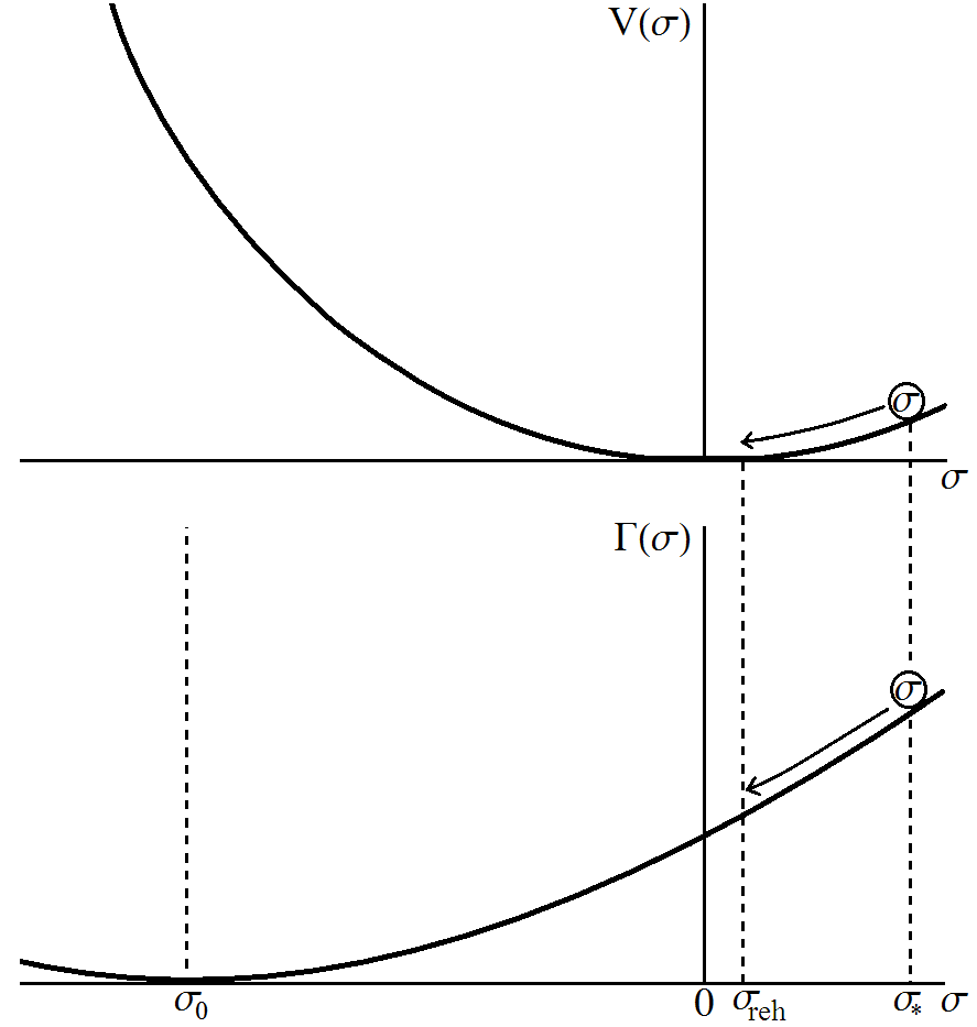
with $\sigma_{*}>\sigma_{0}>0$ (see Figure 1 for an illustration of this model).⁸⁸ 8 The main utility of this model is its simplicity, but it may be possible to realize such a decay rate with a modulus-dependent inflaton mass, $m_{\phi}=m_{\phi}(\sigma)$. An interaction term with a light scalar $\chi$ such as $\mathcal{L}\ni\lambda\phi\chi^{2}$ sources a decay rate $\Gamma\sim\lambda^{2}/m_{\phi}(\sigma)$, which may give rise to a decay rate proportional to $\sigma^{-1}$. Since the modulus field rolls toward $\sigma_{0}$, the decay rate is a monotonically increasing function of time.

With this choice of $\Gamma(\sigma)$, the relationship between $\sigma_{*}$ and $\sigma_{\rm{reh}}$ in Eq.(30) can be approximated as

where $q\equiv\exp\left[{\left(\frac{\mathcal{N_{*}}}{3}-\frac{2}{27}\right)\frac{m^{2}}{H_{*}^{2}}}\right]$ and we have neglected terms of order $m^{4}/\Gamma(\sigma_{\rm{reh}})^{4}$. This equation can be solved analytically as

By substituting Eq.(40) into Eq.(34) for $\mathcal{P}_{\zeta}$, we can obtain an analytic expression for the power spectrum as a function of $\sigma_{*}$. We can further simplify Eq.(40), and thus the formula for $\mathcal{P}_{\zeta}(\sigma_{*})$, in the limit $|X(\sigma_{\rm{reh}})|\gg 1$. First, with the decay rate given in Eq.(38) we obtain

By construction we have $\sigma_{0}<\sigma_{\rm{reh}}<q^{-1}\sigma_{*}$, so

and hence in the limit $|X(\sigma_{\rm{reh}})|\gg 1$, we can reduce Eq.(40) to

Inserting $\sigma_{\rm{reh}}$ into the power spectrum Eq.(34), we finally obtain

We assume the modulus to be light during inflation, $m^{2}/H_{*}^{2}\ll 1$, which implies that $q$ is slightly larger than unity. In contrast, $\mathcal{P}_{\zeta}(\sigma_{*})$ is given by Eq.(33) with $n=-1$ if the modulus dynamics are neglected. We therefore see that the modulus rolling suppresses the power spectrum by a factor that is slightly smaller than $4$ in the limit of large $|X(\sigma_{\rm{reh}})|$. Recall from the discussion following Eq.(25) that we also expect to see $f_{NL}\simeq-10$ in the limit $|X(\sigma_{\rm{reh}})|\gg 1$.

We now adopt the following set of parameters as a definite example for which large values of $|X(\sigma_{\rm{reh}})|$ are realized, and thus the modulus rolling becomes important: {$H_{*}=10^{11}\rm{GeV}$, $\mathcal{N}_{*}=50$, $m=8.6\times 10^{-10}M_{\rm{PL}}$, $\mu=4.5\times 10^{-8}M_{\rm{PL}}$, $\sigma_{0}=4.0\times 10^{-4}M_{\rm{PL}}\}$. We treat the remaining parameter $\sigma_{*}$ as the independent variable. This set is only a representative selection of parameters for which $|X(\sigma_{\rm{reh}})|$ becomes large and it is not the unique set. To obtain this parameter set, we first set a value for $H_{*}$ such that $\mathcal{P}_{\zeta}$ from slow-roll inflaton perturbations can be much smaller than $10^{-9}$ without violating current upper bounds on the tensor-to-scalar ratio. For $|X(\sigma_{\rm{reh}})|\gg 1$, setting the power spectrum from modulated reheating near the observed value ($\mathcal{P}_{\zeta}=2.2\times 10^{-9}$[33]) roughly fixes $(\sigma_{*}-q\sigma_{0})$, as seen in Eq.(44). We then choose values for $\sigma_{0}$, $m/\mu^{2}$, and a parameter range for $\sigma_{*}$ such that $|X(\sigma_{\rm{reh}})|\simeq-20$ and $m^{2}/\Gamma(\sigma_{\rm{reh}})^{2}\lesssim 1$. The modulus mass $m$ is then chosen such that the modulus is light during inflation ($m^{2}\ll H_{*}^{2}$), the modulus energy density is negligible compared to the total energy density ($\rho_{\sigma}\ll\rho_{\rm{tot}}$) before reheating, and the classical rolling of the modulus during inflation dominates over the quantum fluctuations,

where we used the approximate modulus EOM, Eq.(13). Since we also fix a value for $\mathcal{N}_{*}$, the wavelength of the perturbation is uniquely determined by the post-inflation expansion history, which is set by the remaining parameter $\sigma_{*}$. The perturbation scale therefore changes as we vary $\sigma_{*}$. However, the modulus is light during inflation, so the perturbations are nearly scale-invariant, as shown by Eq.(27).

We also set $\beta=1$ in the following calculations so that the time of sudden inflaton decay is defined by $\Gamma(\sigma_{\rm{reh}})/H(t_{\rm{reh}})=1$. Changing $\beta$ mainly results in shifting the e-folding number Eq.(8) by a constant, which does not affect its slope $\mathcal{N}^{\prime}(\sigma)$. Although $\beta$ also alters $\sigma_{\rm{reh}}$ by changing $t_{\rm{reh}}$, we note that the observables $\mathcal{P}_{\zeta}$ and $f_{\rm{NL}}$ are rather insensitive to the precise value of $\beta$, as demonstrated explicitly in Eqs.(44, 25) for the limit $|X(\sigma_{\rm{reh}})|\gg 1$.

Since the modulus’s effective mass is constant for a quadratic potential, the lightness condition is satisfied until $H\simeq m$, which occurs $\frac{2}{3}\ln\left(H_{*}/m\right)=2.6$ e-foldings after inflation in this model. We require the decay condition $\Gamma(\sigma_{\rm{reh}})/H(t_{\rm{reh}})=1$ to be satisfied before the lightness condition is violated, which implies $\Gamma(\sigma_{\mathrm{reh}})\gtrsim m$. Applying this inequality to Eq.(43), we obtain $\frac{2}{27}\sigma_{*}\gtrsim\sigma_{*}-q\sigma_{0}$ which provides us with a maximum value for the parameter $\sigma_{*}$: for the parameters we specified, we have $q=1.007$ and thus $\sigma_{*}\lesssim 1.09\sigma_{0}$. The smallest value of $\sigma_{*}$ we consider must satisfy $\Gamma(\sigma_{\rm{end}})\ll H_{*}$ to ensure that the Universe is effectively matter-dominated prior to reheating; even if $\Gamma$ is constant, the sudden-decay approximation introduces an error to the computed power spectrum that scales with the size of $\Gamma(\sigma_{\rm{end}})/H_{*}$. We restrict our analysis to $\sigma_{*}\geq 1.02\sigma_{0}$ so that the decay rate at the end of inflation is $\Gamma(\sigma_{\rm{end}})\lesssim 0.01H_{*}$.

We plot $X(\sigma_{\rm{reh}})$ as a function of $\sigma_{*}$ in the left panel of Figure 2; we see that $|X(\sigma_{\rm{reh}})|\gtrsim 10$ for the entire $\sigma_{*}$ range of interest. We can understand the behaviour of $X(\sigma_{\rm{reh}})$ pictorially by recalling that $X(\sigma_{\rm{reh}})$ is a measure of $\dot{\Gamma}$ at reheating. We plot $H(t)$ and $\Gamma(\sigma(t))$ for several values of $\sigma_{*}$ near $\sigma_{0}$ in the right panel of Figure 2. Under the sudden-decay assumption, the inflaton decays when the decay condition $\Gamma(\sigma)/H=1$ is satisfied. For the modulus values starting close to $\sigma_{0}$, the inflaton decays before there is significant time for the modulus to roll. As we take $\sigma_{*}$ further from $\sigma_{0}$, however, the initial decay rate $\Gamma(\sigma_{*})$ decreases and the modulus has more time to roll toward $\sigma_{0}$ before the decay condition is satisfied. The decay rate when $\Gamma(\sigma)\simeq H$ is clearly rising more rapidly as we increase the value of $\sigma_{*}$, and therefore the value of $|X(\sigma_{\rm{reh}})|$ increases accordingly as we increase $\sigma_{*}$. Such behaviour can also be understood from the equations: Eq.(41) implies that $X(\sigma_{\mathrm{reh}})$ is a negative and monotonically decreasing function of $\sigma_{\mathrm{reh}}$, as $\sigma_{\mathrm{reh}}>\sigma_{0}$. Furthermore, $\partial\sigma_{\mathrm{reh}}/\partial\sigma_{*}>0$ for a negative $X(\sigma_{\mathrm{reh}})$ [see Eq.(17)]. Hence, the monotonic decrease of $X(\sigma_{\mathrm{reh}})$ as a function of $\sigma_{*}$ is a generic feature of this model, independent of the choice of parameters. The rapid rise of $\Gamma$ at reheating causes the inflaton decay to proceed more rapidly than the usual exponential decay, and we will see that the sudden-decay approximation provides an accurate description of reheating in this scenario.

References

- (1) A. H. Guth, Inflationary universe: A possible solution to the horizon and flatness problems, Phys. Rev. D 23 (1981) 347–356.
- (2) V. F. Mukhanov and G. V. Chibisov, Quantum fluctuations and a nonsingular universe, JETP Lett. 33 (1981) 532–535.
- (3) K. Sato Mon. Not. Roy. Astron. Soc. 195 (1981) 467–479.
- (4) A. H. Guth and S. Y. Pi, Fluctuations in the New Inflationary Universe, Phys. Rev. Lett. 49 (1982) 1110–1113.
- (5) S. W. Hawking, The development of irregularities in a single bubble inflationary universe, Phys. Lett. B 115 (1982) 295–297.
- (6) A. D. Linde, Scalar field fluctuations in the expanding universe and the new inflationary universe scenario, Phys. Lett. B 116 (1982) 335–339.
- (7) A. A. Starobinsky, Dynamics of phase transition in the new inflationary universe scenario and generation of perturbations, Phys. Lett. B 117 (1982) 175–178.
- (8) J. M. Bardeen, P. J. Steinherdt and M. S. Turner, Spontaneous creation of almost scale-free density perturbations in an inflationary universe, Phys. Rev. D 28 (1983) 679–693.
- (9) G. Dvali, A. Gruzinov and M. Zaldarriaga, A new mechanism for generating density perturbations from inflation, Phys. Rev. D 69 (2004) 023505, [astro-ph/0303591].
- (10) L. Kofman, Probing String Theory with Modulated Cosmological Fluctuations, (2003) [astro-ph/0303614].
- (11) M. Zaldarriaga, Non-Gaussianities in models with a varying inflaton decay rate, Phys. Rev. D 69 (2004) 043508, [astro-ph/0306006].
- (12) N. Bartolo, S. Matarrese and A. Riotto, Evolution of Second-Order Cosmological Perturbations and Non-Gaussianity, JCAP 01 (2004) 003, [astro-ph/0309692].
- (13) F. Vernizzi, Cosmological perturbations from varying masses and couplings, Phys. Rev. D 69 (2004) 083526, [astro-ph/0311167].
- (14) T. Suyama and M. Yamaguchi, Non-Gaussianity in the modulated reheating scenario, Phys. Rev. D 77 (2008) 023505, [arXiv:0709.2545].
- (15) K. Ichikawa, T. Suyama, T. Takahashi and M. Yamaguchi, Primordial Curvature Fluctuation and Its Non-Gaussianity in Models with Modulated Reheating, Phys. Rev. D 78 (2008) 063545, [arXiv:0807.3988].
- (16) J. Elliston, D. J. Mulryne, R. Tavakol, What Planck does not tell us about inflation, (2013) [arXiv:1307.7095].
- (17) T. J. Allen, B. Grinstein and M. B. Wise, Non-gaussian density perturbations in inflationary cosmologies, Phys. Lett. B 197 (1987) 66–70.
- (18) T. Falk, R. Rangarajan and M. Srednicki, Dependence of Density Perturbations on the Coupling Constant in a Simple Model of Inflation, Phys. Rev. D 46 (1992) 4232, [astro-ph/9208002].
- (19) A. Gangui, F. Lucchin, S. Matarrese and S. Mollerach, The Three–Point Correlation Function of the Cosmic Microwave Background in Inflationary Models, Astrophys. J. 430 (1994) 447–457, [astro-ph/9312033].
- (20) J. Maldacena, Non-Gaussian features of primordial fluctuations in single field inflationary models, JHEP 05 (2003) 013, [astro-ph/0210603].
- (21) V. Acquaviva, N. Bartolo, S. Matarrese and A. Riotto, Second-Order Cosmological Perturbations from Inflation, Nucl. Phys. B 667 (2003) 119–148, [astro-ph/0209156].
- (22) D. Seery and J. E. Lidsey, Primordial non-gaussianities in single field inflation, JCAP 06 (2005) 003, [astro-ph/0503692].
- (23) P. A. R. Ade, et al. [Planck Collaboration], Planck 2013 Results. XXIV. Constraints on primordial non-Gaussianity, (2013) [arXiv:1303.5084].
- (24) A. A. Starobinsky, Multicomponent de Sitter (inflationary) stages and the generation of perturbations, JETP Lett. 42 (1985) 152–155.
- (25) M. Sasaki and E. D. Stewart, A General Analytic Formula for the Spectral Index of the Density Perturbations produced during Inflation, Prog. Theor. Phys. 95 (1996) 71–78, [astro-ph/9507001].
- (26) D. Wands, K. A. Malik, D. H. Lyth and A. R. Liddle, A new approach to the evolution of cosmological perturbations on large scales, Phys. Rev. D 62 (2000) 043527, [astro-ph/0003278].
- (27) D. H. Lyth, K. A. Malik and M. Sasaki, A general proof of the conservation of the curvature perturbation, JCAP 05 (2005) 004, [astro-ph/0411220].
- (28) T. Kobayashi and T. Takahashi, Large Tensor-to-Scalar Ratio in Small-Field Inflation, Phys. Rev. Lett. 110 (2013) 231101, [arXiv:1303.0242].
- (29) T. Chiba, Slow-Roll Thawing Quintessence, Phys. Rev. D 79 (2009) 083517, [arXiv:0902.4037]. [Erratum-ibid. D 80 (2009) 109902].
- (30) M. Kawasaki, T. Kobayashi and F. Takahashi, Non-Gaussianity from Curvatons Revisited, Phys. Rev. D 84 (2011) 123506, [arXiv:1107.6011].
- (31) C. T. Byrnes and D. Wands, Curvature and isocurvature perturbations from two-field inflation in a slow-roll expansion, Phys. Rev. D 74 (2006) 043529, [astro-ph/0605679].
- (32) T. Kobayashi, F. Takahashi, T. Takahashi and M. Yamaguchi, Spectator field models in light of spectral index after Planck, (2013) [arXiv:1303.6255].
- (33) P. A. R. Ade, et al. [Planck Collaboration], Planck 2013 results. XXII. Constraints on inflation, (2013) [arXiv:1303.5082].
- (34) T. Kobayashi, F. Takahashi, T. Takahashi and M. Yamaguchi, Dark Radiation from Modulated Reheating, JCAP 03 (2012) 036, [arXiv:1111.1336].