Reexamination of Induction Heating of Primitive Bodies in Protoplanetary Disks Note: To appear in ApJ
Abstract
We reexamine the unipolar induction mechanism for heating asteroids originally proposed in a classic series of papers by Sonett and collaborators. As originally conceived, induction heating is caused by the “motional electric field” which appears in the frame of an asteroid immersed in a fully-ionized, magnetized solar wind and drives currents through its interior. However we point out that classical induction heating contains a subtle conceptual error, in consequence of which the electric field inside the asteroid was calculated incorrectly. The problem is that the motional electric field used by Sonett et al. is the electric field in the freely streaming plasma far from the asteroid; in fact the motional field vanishes at the asteroid surface for realistic assumptions about the plasma density. In this paper we revisit and improve the induction heating scenario by: (1) correcting the conceptual error by self consistently calculating the electric field in and around the boundary layer at the asteroid-plasma interface; (2) considering weakly-ionized plasmas consistent with current ideas about protoplanetary disks; and (3) considering more realistic scenarios which do not require a fully ionized, powerful T Tauri wind in the disk midplane. We present exemplary solutions for two highly idealized flows which show that the interior electric field can either vanish or be comparable to the fields predicted by classical induction depending on the flow geometry. We term the heating driven by these flows “electrodynamic heating”, calculate its upper limits, and compare them to heating produced by short-lived radionuclides.
Keywords:
astrobiology — MHD — minor planets, asteroids: general — protoplanetary disksI Introduction
The mineralogy of asteroids inferred from studies of meteorites and asteroid spectroscopy implies that the asteroids were heated during the first few millions years of their lifetimes (e.g., Ghosh et al. 2006 and references therein). The degree of heating depended strongly on heliocentric distance. Igneous-type asteroids at the inner edge of the asteroid belt show signs of heating to 1200 K and are thought to be pieces of the exposed metallic cores of differentiated asteroids (Keil 2000). At the outer edge of the asteroid belt no heating occurred and the asteroids there are thought to be composed of unaltered, primitive solar system materials (McKinnon 1989). Near the center of the asteroid belt, metamorphic type asteroids show mineralogical evidence of aqueous alteration at temperatures of 300–450 K and thermal metamorphism at temperatures up to 1200 K (Keil 2000 and references therein). Some of the asteroids in this region produce fragments which reach Earth in the form of carbonaceous chondrites. The latter may contain innumerable organic compounds, including small amounts of amino acids, the distribution of which depends on the severity of thermal alteration inside the parent body (Glavin et al. 2011). In addition, excesses of L-type amino acids have been found in aqueously altered meteorites (Cronin & Pizzarello 1997; Glavin & Dworkin 2009). Because asteroids may have provided significant amounts of organic material to the early Earth (Chyba & Sagan 1992), understanding how asteroids were heated may be central to understanding the origin of life.
Two theories have been proposed to explain asteroid heating: the decay of short-lived radionuclides (SLRs, Urey 1955) and unipolar induction heating (Sonett et al. 1970). Heating by SLRs such as 26Al is a widely accepted scenario. The discovery of an excess abundance of the daughter nuclide 26Mg in calcium-aluminum rich inclusions (CAIs) from the Allende meteorite implies an 26Al abundance large enough to cause significant heating or even melting (Wasserburg et al. 1977; Lee et al. 1977). However the gradient of heating across the asteroid belt requires a finely tuned dependence of asteroid accretion times on heliocentric distance. For example Grimm McSween (1993) were able to reproduce the observed gradient by assuming that all bodies at each specific heliocentric distance inside the asteroid belt accreted instantaneously, regardless of size, at a time relative to CAI formation determined by the equation
| (1) |
where is an adjustable parameter ranging from 1.5 to 3. Other models have attempted to relax this assumption; however the later models predict that most of the mass of the asteroid belt would be contained in small bodies that would not achieve melting or thermal metamorphism (McSween et al. 2002). This would imply an unobserved excess of small, unheated asteroids in all parts of the asteroid belt. Furthermore, although 26Al heating may have been important in our solar system, the SLR scenario is unlikely to occur elsewhere: Ouellette et al. (2010) predict that the probability of another protoplanetary disk receiving the same concentration of SLRs is only –.
For these reasons we revisit the unipolar induction heating mechanism described in Sonett et al. (1970). In their scenario an asteroid or similarly unmagnetized body is immersed in a uniform, fully-ionized solar wind with velocity , magnetic field , and electric field in the wind’s rest frame. Sonett et al. observed that in the frame of the asteroid there appears a motional electric field,
| (2) |
If the solid body is not a perfect insulator, a nonzero electric field inside it will drive currents which will generate heat via Ohmic dissipation. Sonett et al. calculated the electric field inside the body by treating the latter as a dielectric sphere immersed in a uniform electric field . They assumed that the interior currents are able to form a closed circuit through the plasma and estimated the distortion of the ambient magnetic field by secondary magnetic fields generated by currents in- and around the body. However no attempt was made to account for distortions in the velocity field, , which was assumed to be everywhere.
Unfortunately the classical induction scenario is based on a subtle misconception. Expression (2) is a local relation, in the sense that is the electric field, as measured in the body frame, at the location where the velocity is equal to . Consequently, is the body frame electric field in the freely streaming plasma. If the velocity depends on position, , then the motional field is also position dependent. Thus,
| (3) |
is the motional field at position . Strictly speaking, unipolar induction describes the heating of bodies that do not perturb the velocity field of the surrounding plasma. This is a good approximation in the solar system today,11 1 The unipolar induction mechanism was originally conceived to explain the magnetic fields of the Moon and other bodies in the solar system today (Sonett & Colburn 1968; Schwartz et al. 1969) and later applied to asteroids. where the collision mean free path exceeds the size of any solid body by many orders of magnitude. However the collision mean free path was of order meters in the solar nebula so the distortion of the velocity field cannot be ignored in calculations of asteroid heating. In general, friction between the plasma and body surface will cause the formation of a shear layer, in which decreases systematically to zero at the body surface. It follows that the motional electric field also vanishes at the body surface.
In the following sections we show that, while the motional electric field vanishes on and inside a large body, the total electric field may not. In Section II we give the equations which govern the velocity and electromagnetic fields in and around a body immersed in a flowing plasma. We adopt a multifluid, magnetohydrodynamic description appropriate for weakly ionized protoplanetary disks. In this paper we make no assumptions about the origin of the flow, which could be due to the body’s orbital motion (Weidenschilling 1977a; Morris et al. 2012) or passing shock waves (e.g., Desch & Connolly 2002; Miura & Nakamoto 2006; Hood et al. 2009). Section III describes our disk model and the method used to calculate the abundances of charged particles and transport coefficients in the disk midplane. In Section IV we present two simple examples which show that, although the motional electric field vanishes at the body surface, a non-zero total electric field can exist due to magnetic field gradients in the flow set up by Ohmic dissipation, the Hall effect, and ambipolar diffusion. The effects of small dust grains and possible relevance of our results to asteroid heating are discussed in Section V and our results are summarized in Section VI.
II Multifluid, Magnetohydrodynamic Flow Past an Arbitrary Body
II.1 Governing Equations for the Shear Flow
Consider the flow of plasma past a large, unmagnetized body in a weakly ionized protoplanetary disk. Close to the body surface the plasma is distorted by shearing motions. The dynamics of the shear layer are described by the equations for mass conservation,
| (4) |
momentum conservation,
| (5) |
and energy conservation,
| (6) |
plus the induction equation for a weakly-ionized multifluid plasma,
| (7) |
(Wardle 2007; Balbus 2011), where is mass density, is fluid velocity, is thermal pressure, and is the density of kinetic plus internal energy. The quantity is the net rate of heating () minus cooling () per unit volume due to the absorption and emission of photons, x-ray absorption, cosmic-ray ionization, etc. Strictly speaking, is the velocity of the neutral particles which form the bulk of the weakly-ionized plasma. In Equation (7), is the unit vector parallel to and is the component of perpendicular to . The plasma is described by four transport coefficients: the shear viscosity, , and the diffusivities , , and associated with Ohmic dissipation, the Hall effect, and ambipolar diffusion, respectively.
The solution must satisfy boundary conditions at infinity and also at the plasma-body interface. We work in a frame whose origin lies somewhere inside the body and moves with it. Then the boundary conditions at infinity are
| (8) |
where the subscript “” denotes values in the undisturbed plasma. The free-stream velocity and ambient magnetic field are parameters. The ambient density, pressure, and energy density must be obtained from a model of the protoplanetary disk.
At the plasma-body interface the velocity satisfies the no-slip condition,
| (9) |
and the magnetic induction satisfies
| (10) |
and
| (11) |
(e.g., Jackson 1975), where is the magnetic permeability and is the surface current. The unit normal, , points away from the body and quantities with subscripts b (“body”) and p (“plasma”) are evaluated just in- and outside of the body, respectively, in Equations (10)–(11).
Dimensional analysis of Equations (4)–(7) yields the fundamental length- and time scales for the shear flow. The thickness of the shear layer is predicted to be of order , where
| (12) |
and22 2 It’s important to note that in some cases the Hall diffusivity can be negative (Wardle 2007), in which case the definition given in Equation (13) would not be useful. However we adopt this definition because in our models is positive in the midplane of the disk for all radii of interest.
| (13) |
It is important to note that the scaling for in Equation 12 is appropriate for a dust-free plasma. If dust is present in the disk, the diffusivities and thus will change (See Sections III and V.1). There are three characteristic time scales: the time scale for viscous forces to accelerate the plasma,
| (14) |
the advection time scale,
| (15) |
and the magnetic diffusion time
| (16) |
The scaling in Equations (12), (15), and (16) is appropriate if is the molecular viscosity of the gas (e.g., Schaefer 2010); however the effective viscosity could be much larger if the flow is turbulent. Although the transition from laminar to turbulent flow is not well understood for MHD flow over bodies, this transition has been widely studied for MHD channel flow (Hartmann 1937; Thess et al. 2007 and references therein) and is generally determined by the ratio
| (17) |
of the Reynold number,
| (18) |
to the Hartmann number,
| (19) |
where is the velocity at the center of the channel, is the channel width, and is the Ohmic conductivity of the plasma (See Equation [81]). For MHD channel flow with a uniform magnetic field perpendicular to the walls, the flow is found to remain laminar if the parameter remains less than a critical value determined by both experiments and numerical simulations (Moresco Alboussière 2004; Thess et al. 2007). Although we obviously are not considering MHD channel flow, it seems plausible that the idealized flows over planar body surfaces (See Section IV) considered in this paper may behave similarly. For realistic bodies, will probably depend greatly on the geometry of the flow; however here we will assume that is equal to the above value. If is the molecular viscosity of the plasma, we find that
| (20) |
| (21) |
and hence that
| (22) |
which shows that , suggesting that the flows we study are indeed laminar.
If these flows are in fact turbulent, a larger effective viscosity could be implied. A probable upper limit on is set by assuming that the hydromagnetic turbulence which likely dominates the large-scale dynamics of a protostellar disk extends all the way down to scales of order the body size, . If this were true, would be comparable to
| (23) |
(Shakura Sunyaev 1973), where is a dimensionless number, is the sound speed, is the local disk scale height, and is the local angular velocity. Putting in numbers appropriate for the asteroid belt gives
| (24) |
so that and for bodies of asteroidal size. However even in this highly speculative scenario the time scales in Equations (14)–(16) would all be yr., and therefore steady flow can still be assumed.
The electric field inside the body is coupled to the electric field in the shear layer via boundary conditions at the body-plasma interface (see Equations [31]–[32]); thus it is necessary to calculate the electric field in the plasma. Equation (7), Faraday’s Law, Helmholtz’ Theorem33 3 A vector field is uniquely determined if its divergence and curl are both known., and macroscopic charge neutrality together imply that in a steady flow
| (25) |
Equation (25) says that in general the electric field at each point in the shear flow is the sum of four contributions,
| (26) |
of which the first is the motional E-field. We refer to the other contributions as the Ohm field,
| (27) |
the Hall field,
| (28) |
and the ambipolar field,
| (29) |
because they are the electric fields required to maintain the magnetic field gradients set up by Ohmic dissipation, etc.
The boundary condition on the electric field at infinity is
| (30) |
The boundary conditions at the body-plasma interface are
| (31) |
and
| (32) |
where is the surface charge density, is the dielectric displacement and we assume, for the present, that the dielectric constant, , is a scalar.
II.2 The Body Interior
To calculate the electric and magnetic fields inside the body one must solve Maxwell’s equations there. The light-crossing time for an asteroid of size ,
| (33) |
is utterly negligible compared to the flow time scales (Section II.1), so the fields inside the body are well approximated by Faraday’s Law,
| (34) |
and Ampère’s Law with zero displacement current,
| (35) |
We have assumed that the macroscopic charge density vanishes inside the body and that Ohm’s Law holds with a scalar conductivity . However Equations (34)–(35) make no assumptions about the position dependence of the material properties , , and dielectric constant .
Equations (34)–(35) describe the dissipation of electromagnetic field energy by Ohmic heating of the body material. This can be seen by momentarily neglecting the position dependence of . Then Equations (34) and (35) reduce to diffusion equations for the electric field,
| (36) |
and magnetic field,
| (37) |
In an isolated body, Ohmic dissipation would eventually reduce the electromagnetic field energy in the body to zero. However the electric and magnetic fields in the shear layer and surrounding plasma constitute an energy reservoir which tends to replenish losses inside the body, via the diffusion of and from the plasma into the body. The time to reach a steady state in which diffusive gains balance Ohmic losses is just the diffusion time,
| (38) |
Estimates of depend on the very uncertain electrical conductivities of primitive solar system materials. For example, estimates of for plausible asteroidal constituents span orders of magnitude (Ip & Herbert 1983), and the situation is further complicated if the body contains a spatially connected metallic phase (H. Watson, private communication). Direct measurements of have been carried out for a few chondritic meteorites (Schwerer et al. 1971; Brecher 1973). They are consistent with an Arrhenius-law temperature dependence,
| (39) |
with and eV. In the absence of more extensive measurements we will adopt these values, giving
| (40) |
over the temperature range – K. Given the shortness of the times in Equation (40), it seems reasonable to neglect the time dependence of and , uncertainties in notwithstanding. Then Faraday’s Law reduces to
| (41) |
i.e., finding inside the body reduces to a boundary-value problem in electrostatics. Once is known, Ampère’s Law reduces to a set of coupled ordinary differential equations for . In Sections IV.1–IV.2 we show how this all works out for two extremely simple models.
II.3 Self Heating
Dissipative processes inside the shear flow transform ordered kinetic energy into heat. Since the transport coefficients depend on temperature, it is important to know whether the heating is large enough to raise the temperature above ambient. The friction associated with viscosity heats the plasma at a rate
| (42) |
where is the viscous stress tensor and is the velocity gradient tensor. In Cartesian coordinates
| (43) |
and
| (44) |
Taking and gives the order-of-magnitude estimate
| (45) |
Notice that the RHS of Equation (45) is independent of the viscosity.
The shear flow is also heated by the friction associated with streaming motions between charged and neutral particles; however electron-neutral scattering can generally be neglected (Balbus 2011). Let be the number density of ions with mass and charge and be the number density of neutral particles with mass . If or is nonzero, the ions will be accelerated by the Lorentz force. On a very short time scale they reach a terminal velocity with respect to the neutrals, such that the Lorentz force is balanced by the drag force associated with elastic ion-neutral scattering. The terminal drift velocity is
| (46) |
(Wardle 1998), where is the ion velocity and
| (47) |
is the electric field in the frame of the neutral particles (=the bulk plasma). The drift velocity depends on the dimensionless ion Hall parameter,
| (48) |
where
| (49) |
is the ion cyclotron frequency,
| (50) |
is the time scale for the ions to reach their terminal drift speed, and is the momentum transfer rate coefficient for elastic ion-neutral scattering. Ion-neutral streaming heats the neutral gas at a rate
| (51) |
(Draine et al. 1983; Chernoff 1987), where is the ion-neutral reduced mass.
III Transport Coefficients
In Section IV we present analytic solutions which describe shear flow past an infinite slab. These solutions are cast in dimensionless units which depend only on certain combinations of the transport coefficients. However to express the solutions in terms of ordinary units we require numerical values of , , , and . We estimate these as follows.
III.1 Protoplanetary Disk Model
We use the density and temperature predicted by the minimum mass solar nebula (MMSN) model (Weidenschilling 1977b; Hayashi 1981) as described by Sano et al. (2000). The gas temperature is
| (52) |
where is distance from the central star. The mass density is
| (53) |
where is vertical distance from the midplane. The midplane density of the MMSN is
| (54) |
where is the mass of the central star, is the mean mass per neutral particle, and is the hydrogen mass. We set and , the latter corresponding to a gas composed of molecular hydrogen and helium with number densities and , respectively, where is the number density of hydrogen nuclei. Then the gas number density at the midplane is
| (55) |
The midplane temperature and number density are plotted versus in Figure 1. We also require the ambient magnetic field, . It is not yet possible to directly measure the magnetic fields in protoplanetary disks; however several lines of evidence suggest that – G, including simulations of star formation (Desch & Mouschovias 2001) and constraints implied by protostellar mass accretions rates (Wardle 2007; Bai & Goodman 2009). We will adopt the value G for our calculations discussed in Section V which is approximately the geometric mean of the extremes.
III.2 Ionization Equilibrium
The magnetic diffusivities depend on the number densities of ions, electrons, and charged dust grains (Section III.3). To estimate these we use the semianalytical model of ionization equilibrium developed by Okuzumi (2009). Okuzumi’s model calculates the number densities of electrons, dust grains in different charge states, plus the total ion number density,
| (56) |
where the sum is over different ionic species . Okuzumi’s results are in excellent agreement with full numerical calculations in which different ionic species are treated explicitly.44 4 See Okuzumi (2009) Figure 3 but note that the figure has an error: the code which plotted Figure 3b multiplied every quantity by a factor of (S. Okuzumi, private communication). The inputs to Okuzumi’s model are listed in Table 1, where
| (57) |
is the average recombination rate coefficient of the ions,
| (58) |
is the average of the mean ion thermal speed, and
| (59) |
where is the number of ionizations per unit volume per unit time and the sum is over all gas-phase species . More detailed treatments of ionization equilibrium in disks (e.g., Sano et al. 2000) show that the abundance of atomic ions exceeds the abundance of molecular ions by 2–3 orders of magnitude. We will take Mg+ to be a proxy for the ions and set
| (60) |
where , and
| (61) |
which is the rate coefficient for radiative recombination of Mg+ (McElroy et al. 2013).
The ionization rate, , is crucial but uncertain. In a protoplanetary disk it has contributions from cosmic rays, x rays, and live radionuclides so that
| (62) |
The cosmic ray ionization rate is
| (63) |
where is the rate far from the midplane. The factor
| (64) |
describes attenuation by the gaseous disk (Okuzumi 2009), with
| (65) |
| (66) |
and g cm-2. Here we are interested only in points with so that
| (67) |
where
| (68) |
is the total surface density. Since the cosmic ray ionization rates of H2 and He are the same to within about 20%, we will take to be the rate for molecular hydrogen. Values of the latter inferred from observations of molecular clouds span about two orders of magnitude, from s-1 to s-1 (Padovani et al. 2009 and references therein). We will adopt the value suggested by Dalgarno (2006),
| (69) |
which is approximately the geometric mean of the extremes.
Our models also include ionization by stellar x rays and radionuclides. For the former we adopt the fit of Turner & Sano (2008) to calculations of x-ray ionization by Igea & Glassgold (1999):
| (70) |
where g cm-2, s-1, and the stellar x-ray luminosity, , is a parameter (Table 1). The rate of ionization by radioactivity depends strongly on the presence or absence of short-lived radionuclides (SLRs) like 26Al. It increases from s-1 if SLRs are absent to s-1 if SLRs are present with the abundances inferred for the early solar nebula (Umebayashi & Nakano 2009). The fact that chondrules are a few Myr younger than the first solids to condense from the solar nebula (the CAIs) suggests that the solar nebula was a few Myr old when the asteroids formed, at least for the parent bodies of chondritic meteorites. Since the half life of 26Al is 0.7 Myr, we will neglect ionization by SLRs. The midplane ionization rates are plotted vs. in Figure 2.
The ionization balance and magnetic diffusivities are sensitive to the presence of small (with radii less than a few µm) dust grains. Dust tends to sweep up electrons, the only particles that are well coupled to at the densities of interest here (Section III.3). This reduces the coupling between gas and magnetic field with a consequent increase in the diffusivities. For example Wardle (2007) showed that a standard interstellar population of grains with µm would increase the diffusivities enormously, by orders of magnitude in the midplane. However grain growth can reduce the total dust surface area55 5 If the grains grow as spheres with fractal dimension . However the initial stages of grain growth generally produce fractal structures with (Blum & Wurm 2008 and references therein). To be consistent with the grain model of Birnstiel et al. (2011) considered below [see Equation (71)] we will set . to a point where the effect of grains on the diffusivities becomes negligible; Wardle (2007) showed that (for nonfractal grains) this occurs when exceeds a few µm. In this paper we are concerned with disk ages of a few Myr, which is longer than the time scale for grain growth (Dullemond & Dominik 2005). The expectation that grain growth is significant at Myr is borne out by millimeter observations of disks, which suggest that most of the dust is locked up in millimeter and larger-size particles at about Myr (Williams 2012 and references therein). However Spitzer observations of the infrared features produced by amorphous (at µm) and crystalline ( µm) silicates imply the presence of µm-sized grains in numerous disks (e.g., Furlan et al. 2011). Because these disks are optically thick the observed small grains lie in the disk atmospheres, i.e., not in the midplane. Nevertheless, it is important to know whether enough µm-sized dust might reside in the midplane to affect the diffusivities.
To estimate the density of small dust at the midplane we exploited the calculations of Birnstiel et al. (2011), who described the equilibrium size distribution established by coagulation and fragmentation. Birnstiel et al. modeled a grain of radius as a constant-porosity sphere of mass
| (71) |
where is the bulk density of the porous solid. At any given time the mass distribution extends from the monomer mass, , to some upper limit, , determined by the growth process. For a range of models with different assumptions about the underlying physics they found that the mass distribution can be approximated by a power law66 6 Strictly speaking, the distribution given in Equation (72) does not account for the effect of settling in disk. However numerical simulations performed by Birnstiel et al. (2011) including the effects of settling and turbulent mixing find that the vertically integrated dust distribution can be approximated by two power laws depending on whether or not the radius of the grains are greater than a certain size (See their Section 3.2 and Figure 4).,
| (72) |
where is the number density of grains with masses in and lies in the range from about to . We set and , where µm and mm, corresponding to the coagulation of interstellar dust to sizes consistent with the millimeter observations of disks. The total abundance of dust with all sizes is characterized by , where is the total dust mass density and . As a measure of how much small dust is present we define to be the mass density of dust with radii less than . Then it is easy to show that Equation (72) implies
| (73) |
Figure 3 plots for a few plausible values of . It is apparent that the theory allows a very broad range in the mass fraction of micron-size and smaller grains, from to .
Figure 4 plots the abundances of ions, electrons, , and relative to calculated using Okuzumi’s model as a function of in the disk, assuming . Here and describe the total amount of positive and negative charge contained by dust grains, and are defined as
| (74) |
and
| (75) |
where is the charge of the grains in the units of elementary charge. We assume that all the dust grains are single-sized with radius and consider two cases: µm and . When µm we find that positively and negative charged dust grains are the dominant charge carriers in the plasma for AU. For AU, negatively charged dust grains still dominate over electrons while ions become the dominate carrier of positive charge. When AU, ions and electrons become the dominant charged species. If the grain radius is increased to µm , we observe that the abundances of ions and electrons exceed those of charged dust grains for all AU. For 1 1.5 AU, negatively charged dust grains become more abundant than electrons in the plasma while ions continue to be the dominate carrier of positive charge.
Of particular interest to the flows considered in this paper is the electron abundance,
| (76) |
since the electrons are the only particles that are strongly tied to the magnetic field (See Section III.3). The effects of dust on the electron abundance in the midplane of the disk are shown in Figures 5 and 6. The calculations were carried out for two values of toward the high end of the plausible range and assumed single-size grains. The electron abundance in a dust-free plasma is also shown for comparison. The figures confirm that is very sensitive to the abundance of the smallest grains in the distribution if the latter are smaller than a few µm (Wardle 2007). For example, the electron abundance is reduced by about three orders of magnitude at AU if µm and (Figure 5). However once the abundance of small dust falls to the effects of dust are small unless µm (Figure 6). We will calculate the diffusivities for two cases: a dust-free plasma and a plasma with , µm. However it should be kept in mind that, if the power-law grain size distribution is steeper than , our calculations will underestimate the diffusivities by orders of magnitude.
III.3 Viscosity and Magnetic Diffusivities
The shear viscosity depends only on temperature. We adopt the viscosity values calculated by Schaefer (2010), which are well approximated by
| (77) |
for both ortho- and para-H2 if K.
The magnetic diffusivities are obtained from the charged particle abundances as follows (Wardle 2007):
| (78) |
| (79) |
and
| (80) |
where
| (81) |
is the Ohmic conductivity,
| (82) |
is the Hall conductivity,
| (83) |
is the Pedersen conductivity, and . The sums are over all charged species with mass , number density , and charge . We include electrons, ions, and single-size grains in various charge states. In particular we include all grain charge states within four standard deviations of the mean charge (see Okuzumi [2009]).
In addition to the abundance of each charged particle, the diffusivities depend on its dimensionless Hall parameter, which depends in turn on its drag time, . The latter is defined by the drag force produced by friction with the neutral gas:
| (84) |
For the ion drag time we adopt Equation 50 with cm3 s-1 and for the electrons we use
| (85) |
with
| (86) |
and cm2 (Draine et al. 1983). For the drag force on dust grains we use the expression given by Draine & Salpeter (1979) in the limit of subsonic gas-grain drift. It implies that
| (87) |
where
| (88) |
The coupling between each charged particle and the magnetic field is characterized by . If then species is well coupled to the magnetic field lines and moves with them. If for all charged species the magnetic field is frozen into the charged particles and we recover ideal MHD. The Hall parameters of the electrons, ions, and dust grains with µm are plotted vs. in Figures 7 and 8 for two different values of . The model adopted here predicts and over the region corresponding to the asteroid belt; this is the Hall regime where the electrons move with but the ions do not. Notice that the dust Hall parameter is extremely small so that the terms corresponding to dust in the sums for the conductivities are negligible if µm. This will hold unless very small grains with Å are present as free fliers in the plasma, a scenario we do not consider here. Nevertheless, dust affects the diffusivities profoundly by reducing the gas-phase abundances of the electrons and ions. The diffusivities are plotted in Figures 9 and 10 for (no small dust), , and two plausible values of the magnetic field .
III.4 Another Ionization Model
To illustrate the dependence of the magnetic diffusivities on our specific disk model, we now compare our ionization and magnetic diffusivity calculations to another model described in the recent work of Dzyurkevich et al. (2013). Although the model used by Dzyurkevich et al. makes similar assumptions about the physical conditions (i.e., density, temperature, magnetic field) in the disk, they make significantly different assumptions regarding the ionization rates and properties of the dust grains. The most important difference between our models is the assumed fractal dimension of the grains, which Dzyurkevich et al. set equal to 2 corresponding to grains modeled as fluffy fractal aggregates. In addition, Dzyurkevich et al. assume a smaller ionization rate (by about an order of magnitude) and introduce the concept of a “metal line” in the disk, beyond which metal ions freeze out and molecular ions become the dominant ionic species. In order to make a quantitative comparison between models, we now calculate the abundances of charged particles and magnetic diffusivities as a function of for the model described by Dzyurkevich et al. (2013). The parameters used in these calculations are listed in Table 2, where we note that in order to recreate the results described in their paper, we required a total magnesium abundance relative to hydrogen nuclei in the disk of , which is 100 times larger than the value quoted in their Appendix B.
Figures 11–12 show the abundances of ions, electrons, and charge contained on dust grains, as well as the magnetic diffusivities in the disk midplane for the model described by Dzyurkevich et al. (2013). In the left panel of Figure 11, we find that the dominant charge carriers are positively- and negatively-charged dust grains for AU, ions and negatively-charged dust grains for AU, and ions and electrons for AU. For completeness we also plot the specific abundances of and in the right panel of Figure 11, which demonstrates the effect of the “metal line” in this disk model. Comparing Figure 11 with Figure 4, we find that although the ionization is qualitatively similar, the total fractional ionization predicted by our model exceeds that predicted by the model described by Dzyurkevich et al. by about 2 orders of magnitude. As expected, this leads to a large difference in the predicted values of the magnetic diffusivities. Comparing Figure 12 with Figure 10 we find that although the Hall diffusivity is largest for AU in both models, in general the values of the magnetic diffusivities are larger by orders of magnitude for the model described by Dzyurkevich et al. (2013). The main effect of larger magnetic diffusivities in the disk is just to increase the thickness for the shear layer (See Section V.2).
IV Steady Flow Past an Infinite Slab
Given the complexity of the governing equations, it seems inevitable that flows around bodies with realistic shapes will have to be calculated numerically. Here we consider a highly idealized problem— steady flow past an infinite slab (Figure 13)— which can be studied analytically. Although the geometry is unrealistic, the solutions illustrate how the the electric field inside a body couples to the flow around it. In this section we will assume that self heating of the shear flow is insignificant, so that the temperature at each point in the flow equals the temperature of the undisturbed plasma and the energy equation can be omitted; the validity of this assumption is checked in Section V.2. Since mass is conserved identically in a steady shear flow, it is only necessary to solve the momentum and induction equations for , , and , plus and Ampère’s Law for and .
IV.1 Parallel Field Geometry
We consider first the simplest possible case, where the ambient magnetic field is parallel to the body surfaces: . For the shear flow we assume that
| (89) |
| (90) |
and that the pressure is constant. Under these assumptions, the induction equation is satisfied identically and the momentum equation reduces to a single ODE for ,
| (91) |
with boundary conditions
| (92) |
and
| (93) |
Symmetry requires to be an even function of , so it is only necessary to calculate the solution explicitly for .
The electric field inside the body can be calculated exactly. Outside the body the magnetic field is simply advected by the flow. Since there is no compression or bending of the field lines, the magnetic field is uniform with everywhere. It follows that the Ohmic, ambipolar, and Hall electric fields all vanish in the plasma and hence that equals the motional field. Now the no-slip boundary condition implies that just outside each body surface. We find the electric field just inside each surface by applying the boundary conditions across the plasma sheath, whose thickness is neglected because it is of order meters and thus much less than the dimensions of the shear layer. Using Equations (31) and (32) with , we find
| (94) |
where the upper and lower signs correspond respectively to the upper and lower slab surfaces. The two electric fields in Equation (94) are just the electrostatic fields associated with electric charge in the plasma sheaths at the upper and lower surfaces; their existence and potential consequences for heating are not the subject of this investigation. In any case, the sum of the “sheath fields” vanishes for the geometry considered here: In order to satisfy and everywhere inside the body each sheath field must be uniform (for an infinite slab), so that Equation (94) is actually valid throughout the body interior. But the sheath fields sum to zero so the total electric field inside the body is . We conclude that it is possible for induction heating to vanish when one accounts for the interaction of a body with the flow around it. Of course the fact that exactly is a consequence of the extreme symmetry of an infinite slab. For realistic bodies of finite extent the electric field will not be zero, but instead attain some value dependent on the nonzero magnetic field gradients associated with departures from planar symmetry.
The electric field in the plasma must vary continuously with , from at infinity to zero at the slab surfaces. One could calculate in principle from the velocity solution by evaluating
| (95) |
However it is well known that the solution for does not exist for an infinite plane: the solution to Equation (91) cannot satisfy boundary conditions (92) and (93) simultaneously because the shear layer is infinitely thick. Since the magnetic forces vanish for this geometry, a rough picture of the variation can be obtained by considering viscous flow past a semi-infinite flat plate, for which the shear layer has finite thickness . Then the boundary condition at infinity can be replaced by
| (96) |
From scaling arguments, Blasius (1908) inferred that
| (97) |
for flow past a semi-infinite plate, where is the distance downstream from the leading edge of the plate. The thickness of the shear layer varies with but the rate of change,
| (98) |
goes to zero as . Thus, becomes approximately independent of for large and the flow approximates flow past an infinite slab. We will interpret in Equation (96) to be , where is a large but unspecified value of for which the approximation holds to some desired precision. Then the solution to Equation (91) subject to the approximate boundary conditions (93) and (96) is
| (99) |
and the electric field in the plasma is
| (100) |
That the electric field in Equation (100) has nonzero divergence shows that the approximation for is unphysical. However the nonzero macroscopic charge density implied by Gauss’s Law is
| (101) |
which goes to zero as .
IV.2 Perpendicular Field Geometry
Now consider the case where the ambient magnetic field is perpendicular to the slab faces, with . Because the slab is infinite all variables depend only on and the electric field can be calculated trivially. Far from the body, where magnetic field gradients vanish, the electric field in the body frame is just the motional field with components77 7 Looking at the velocity and magnetic field solutions in Equations (130)–(133), we note that the motional electric field in the plasma also contains an unphysical non-zero -component () in this case. However is found to be of order , which is and is therefore neglected.
| (102) |
For steady flow the electric field at an arbitrary point in the plasma88 8 To avoid numerous disclaimers we imply henceforth that “in the plasma” means points in the plasma outside of plasma sheaths. must also satisfy which, together with the fact that only depends on , implies that everywhere in the plasma. Now the electric field inside the body is also uniform because and . Noting that is tangent to the slab surfaces, and that the tangential component of does not change across the surfaces, we see that everywhere inside the body, and hence that everywhere. This simple example shows that it is possible to have electric fields inside the body. In the following subsections we show how this is physically possible by calculating the motional, Ohm, Hall, and ambipolar contributions to .
IV.2.1 The Body Interior
For infinite planar geometry the condition implies that is constant, so
| (103) |
We assume a solution of the form , where the notation indicates that and are regarded as small perturbations: . This is necessary because the - and -components of the magnetic field are small outside of the slab (Section IV.2.2) and it would not be possible to satisfy the boundary conditions on at the slab surfaces, in general, if the components of the magnetic field were small outside and large inside. Because is known, and follow from Ampère’s Law. Writing out the and components of Equation (35) gives
| (104) |
and
| (105) |
where it has been assumed for convenience that is constant and is the electrical conductivity inside the body. It is apparent from the symmetry of the problem that and must either be odd or even functions. However even functions are excluded: is odd outside the body (Section IV.2.2) and it would not be possible to satisfy the boundary conditions at the body surfaces in general if were even inside and odd outside. The boundary conditions on Equations (104)–(105) are therefore
| (106) |
and
| (107) |
The solution of Equations (104)–(107) is
| (108) |
and
| (109) |
where we have exploited the fact that everywhere. In practice Equation (108) sets an upper limit on the conductivity, above which our treatment of as a perturbation would break down. The conductivity appears inside the integral in Equation (108) to allow for the sensitive dependence of on the temperature (Equation [39]), which varies with if the body is heated significantly.
IV.2.2 The Shear Flow
Now consider the velocity and magnetic field in the plasma. We seek solutions to Equations (5) and (7) of the form
| (110) |
| (111) |
and , where we have anticipated that the magnetic field is deflected only slightly and regard and as infinitesimal perturbations. Substituting the assumed solutions into Equations (5) and (7), setting the time derivatives to zero, and retaining terms up to first order in and yields six differential equations for the components of and . However the component of the linearized induction equation is satisfied identically. The component of the linearized momentum equation reduces to an equation for the pressure gradient required to maintain hydrostatic equilibrium in the direction; it decouples from the other equations when the temperature dependence of the transport coefficients is neglected. This leaves four ODEs for , , , and :
| (112) |
| (113) |
| (114) |
and
| (115) |
It follows from Equations (112)–(115) that and are even functions of and that and are odd. Thus it is only necessary to calculate the flow explicitly for .
Equations (112)–(115) contain the second derivatives of , , , and so that eight boundary conditions are required. At the body surface the velocity satisfies the no-slip condition,
| (116) |
| (117) |
and the tangential components of the magnetic field satisfy Equation (10):
| (118) |
and
| (119) |
Far from the body the velocity approaches the free-stream velocity,
| (120) |
| (121) |
and the magnetic field perturbations approach constant (infinitesimal) values:
| (122) |
and
| (123) |
For a body of finite size and would vanish at infinity. However our infinite planar slab acts as an infinite current sheet; thus it produces a magnetic field whose magnitude is constant everywhere outside the body.
We introduce the dimensionless position , velocity, , and magnetic induction, , where
| (124) |
is the natural unit of magnetic induction. In dimensionless units Equations (112)–(115) become
| (125) |
| (126) |
| (127) |
and
| (128) |
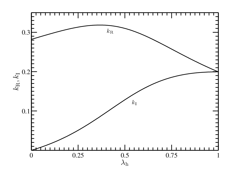
where primes indicate derivatives with respect to . Apart from the boundary conditions the exterior solution depends on just one dimensionless parameter,
| (129) |
which varies from zero (no Hall effect) to unity (Hall effect only, no Ohmic dissipation or ambipolar diffusion). Figures 14–15 show the value of as a function of for two cases: the dust-free case, and the case where and the dust is assumed to be single-sized with m. We point out that in both cases the shear flows are “Hall dominated” in the sense that for most radii of interest.99 9 Although the Hall effect dominates the dynamics of the flows studied here, this may not be the case for other flows, particularly in the context of the magnetorotational instability (MRI; Balbus & Hawley 1991). For example, 3D numerical MHD simulations done by Sano & Stone (2002) show that the Hall effect may be neglected when determining the condition for MRI turbulence, even though the value of the Hall diffusivity may exceed that of the Ohmic and ambipolar diffusivities.
Equations (125)–(128) are solved in Appendix A, where we show that
| (130) |
| (131) |
| (132) |
and
| (133) |
where
| (134) |
is dimensionless height above the body surface and
| (135) |
The solution depends on via the dimensionless quantitities
| (136) |
and
| (137) |
(Figure 16), where
| (138) |
and
| (139) |
Notice that and . Now that the flow velocity and magnetic field solutions are known, the motional, Ohm, Hall, and ambipolar components of the electric field can be found by evaluating Equations (26)–(29). These fields will be discussed in the next section.
V Discussion
V.1 Electric Fields in Multifluid Shear Flows
As demonstrated in the previous section, the solutions for the velocity, magnetic, and electric fields depend only on the transport coefficients , , , and . Although the shear viscosity does not depend on the amount of small dust in the disk, dust may profoundly affect the diffusivities (see Section III.3, Figures 9–10). In order to illustrate the effects of dust on the components of the electric field we will consider two cases: (1) the limit where all the dust is locked into millimeter or larger grains and their is no small dust present in the disk () and (2) a case where the abundance of small grains is taken to be and all the small dust is the same size with a radius of m.
Figures 17–18 describe the electric field in a perpendicular shear flow when no small dust (=0) is present in the disk. These electric fields were computed using our disk model (Section III) where the diffusivities were calculated at AU assuming G. The plots are independent of because is plotted in units of . The motional, Ohm+ambipolar1010 10 The sum of the Ohm and ambipolar E fields is plotted because, for perpendicular geometry, they are proportional to one another. and Hall electric fields are indicated and the total field is also plotted. The figures show the inevitable result that . What is interesting about the figure is how this result comes about. The Ohm and ambipolar fields are relatively small. The motional field dominates far from the body and the Hall field dominates close to the body. For a body of realistic shape the four contributions to the electric field would obviously not “conspire” to sum to as in Figures 17–18. However since the magnitudes of the various magnetic field gradients should not be very sensitive to body shape (for large bodies), it seems clear that real shear flows will have electric fields .
If small dust is present in the disk, the diffusivities and thus the electric field will be affected. Figures 19–20 describe the electric field for the case analogous to Figures 17–18 except with and m. Comparing Figures 19–20 with Figures 17–18, it is evident that even with small dust with abundances as high as present in the disk, the flow remains Hall-dominated at AU with a total electric field . However dust does produce a dramatic effect on the characteristic length scale of the shear layer , which grows from km in the absence of small dust to km when small dust is present. This effect is important to note because our approximation of the asteroid as an infinite plane is only valid when . Taking km for a typical large asteroid, we find that our solutions should provide a decent approximation in a dust-free plasma, however their validity should be questioned when µm-sized dust is present in the abundances discussed above. In the extreme case that µm dust grains are present in the midplane, the magnetic diffusivities will be even greater corresponding to an even larger characteristic length scale of shear layer and rendering our approximation of an asteroid as an infinite plane completely unrealistic. In this case numerical calculations of the flow over a finite body would be required.
V.2 The Importance of Self Heating
In Section IV.2 we solved the equations of motion for a multifluid shear flow on the assumption that heating of the flow by viscous dissipation and ion-neutral scattering is negligible. This will be a good assumption if the heating rates are , where is the radiative cooling rate of the plasma.
V.2.1 Radiative Cooling
In the absence of dust, radiative cooling is mainly due to rotational and vibrational transitions of H2, CO, and H2O molecules. We calculate the cooling rate due to molecular line emission by interpolating the results given by Neufeld Kaufman (1993) at several values of . These cooling rates depend on the velocity gradients in the plasma, which determine the probability that an emitted photon has of escaping (See Neufeld Kaufman 1993). Since the viscous dissipation and ion-neutral scattering heating rates are greatest at the asteroid surface (See Equations [148] and [152] below), we use the velocity gradients in the shear flow
| (140) |
at the body surface (). The radiative cooling rates also depend strongly on the abundance of water vapor in the gas, which may freeze out. Since the location of the snow line in protoplanetary disks is still a topic of active research (e.g., Martin Livio 2012 and references therein), we assume that the abundance of water is constant for all and calculate the cooling rate for two cases: (Figures 21–22) corresponding to a standard abundance water in the gas phase, and (Figures 23–24) assuming that all the water has frozen out.
If dust is present, its thermal emission will also contribute to the cooling of the plasma. It is easy to show that the shear layer is optically thin to the dust thermal emission, and thus the dust radiative cooling rate is
| (141) |
(Draine 2011) where is the Stefan-Boltzmann constant, is the dust temperature, and is the dust grains’ Planck-averaged emission efficiency with
| (142) |
The cooling rate due to dust thermal emission is plotted as a function of in the disk in Figure 25, assuming that the dust grains are a single-size distribution with µm and .
V.2.2 Self Heating Rates
The heating rate due to viscous dissipation can be calculated by evaluating Equation 44 using the velocity solution given in Equations 130–131. For the shear flow considered in Section IV.2, the components of the viscous stress tensor become
| (143) |
| (144) |
| (145) |
and
| (146) |
Substituting these stresses into Equation (44) gives
| (147) |
Using the solutions found in Section IV.2 to calculate the derivatives of and and substituting them into the equation above gives
| (148) |
In addition to the viscous dissipation heating rate, the heating rate in the shear flow due to friction between the ion and neutral fluids can also be calculated. Substituting the assumed forms of the plasma velocity, magnetic, and electric fields described in Section IV.2 into Equation (46), the ion-neutral velocity differences are found to be
| (149) |
| (150) |
and
| (151) |
The ion-neutral frictional heating rate is
| (152) |
Upon inspection of Equations (148) and (152), it is clear that the heating rates due to viscous dissipation and ion-neutral scattering depend strongly on the free-stream velocity of the plasma and are largest at the asteroid surface (). In order to assess the importance of self heating, we consider flows with km/s and km/s, which could correspond to flows driven by the relative motions between the asteroid and the gas on an eccentric orbit (Morris et al. 2012) or a passing shock wave in the disk. As done in the previous section, we present two cases: the dust-free case, and the case where with m.
Figure 26 describes the heating rates due to viscous dissipation and ion-neutral scattering at the body surface as a function of in a dust-free plasma. The left and right panels describe flows with km/s and km/s respectively, and assume G. For both flows we note that the heating rate due to viscous dissipation dominates that of ion-neutral scattering at all distances of interest. Comparing the heating rates (Figure 26) to the radiative cooling rates when gas-phase water is present in the abundance (Figure 21), we observe that for flows with km/s the cooling rate exceeds the heating rate for 4 AU. For 6 8 AU, the heating and cooling rates become comparable. If the free-stream flow velocity is increased to km/s, the cooling rate still dominates the heating rate for AU. Once AU, the heating and cooling rates become comparable. For AU, we find that the heating rates start to exceed the cooling rate. Thus we conclude that self heating of the plasma is insignificant for flows with km/s at 6 AU. However for faster flows with free-stream velocities km/s, significant self heating of the plasma to temperatures above ambient (Equation 52) may become important, particularly at 3 AU. If gas-phase water is absent in the disk, the heating rate is found to exceed the cooling rate (Figure 23) at all for both and km/s, implying that significant self heating of the plasma would occur.
Figure 27 shows the analogous heating rates in the case were single-sized small dust grains are present in the disk with an abundance and radius m. Once again we note that viscous dissipation dominates the heating at all considered values of . Comparing the heating rates (Figure 27) to the cooling rates by dust thermal emission (Figure 25) and molecular line emission (Figures 22) when a standard abundance of gas-phase water is present in the disk, we find that the cooling rate exceeds the heating rate at all for km/s. Under these conditions, dust emission dominates the total radiative cooling rate of the plasma for AU, but becomes insignificant for AU. For faster flows with km/s, the cooling rate is again found to exceed the heating rate for AU. In this case dust thermal emission again dominates the cooling for AU, but becomes smaller than the rate of cooling by molecular line emission for AU. If gas-phase water is absent, the cooling rate becomes dominated by thermal dust emission at all of interest for both and km/s. Comparing the heating rates to the cooling rate due to dust emission, we find that the cooling rate exceeds the heating rate everywhere for km/s. For faster flows with km/s, the cooling rate still exceeds the heating rate for AU. However for AU, the heating rate is found to exceed the cooling rate, implying that significant heating of the plasma would occur.
V.3 Chiral Asymmetry and the Hall Effect
As noted by Wardle (2007), the Hall effect is capable of imparting a handedness to multifluid MHD. Using our velocity solutions calculated in Section IV.2, we demonstrate this feature and the resulting chiral asymmetry in the plasma flow. Outside the shear layer the neutral velocity is just the free-stream velocity . Inside the shear layer, however, the velocity vector rotates. As shown in Figure 28, if the unperturbed magnetic field points in the -direction the velocity rotates counterclockwise in the - plane and acquires a component , which is positive near the body surface. However, if points in the -direction, the velocity rotates clockwise through the same angle in the - plane and acquires a component , which is negative close to the body. As is clearly seen in Figure 28, these rotations define a chiral asymmetry in the neutral velocity profile which depends on the relative orientation of and .
The observed chiral behavior of the flow can be explained by considering the motions of the neutral and charged particles. Since electromagnetic forces do not act directly on the neutral (bulk) plasma and the electron-neutral collisional force is neglected, the only force that can be responsible for producing the neutral velocity component is drag between ions and neutral particles. In the absence of the Hall effect, the ions and electrons flow together in the -direction. However if the Hall effect is present, the Lorentz force causes the ions and electrons to move relative to one another in the -direction. Assuming macroscopic charge neutrality () in the flow, this relative motion between the ions and electrons defines a component of the current density in the -direction given by
| (153) |
This component of the current density is associated with a gradient in the -component of the magnetic field through Ampère’s Law
| (154) |
which produces a -component of the magnetic tension force
| (155) |
For weakly ionized plasmas the ion-neutral drag force can generally be written as
| (156) |
(e.g., Balbus 2011), where . Substituting Equation (154) into Equation (156) and looking at the -component of the equation gives
| (157) |
which shows that as the magnetic tension force pushes the ions in the -direction, they drag the neutral particles with them. Thus, when the free-stream velocity of the neutral particles () points in the -direction and the undisturbed magnetic field () points in the -direction, magnetic tension due to the Hall effect forces the ions to move and drag the neutral particles with them in the -direction, causing the flow to rotate in the counterclockwise direction; while if the direction of is reversed and now points in the -direction, magnetic tension due again to the Hall effect forces the ions and neutral particles to move in the -direction, causing the flow to rotate in the clockwise direction. As shown by the solutions in Section IV.2, this component of the neutral velocity outside of the plane defined by the directions of and can be large and thus cannot necessarily be treated as a perturbation in MHD planar shear flow analysis.
V.4 Electrodynamic Heating
Although the motional electric field decreases to zero at the surface of a large body, Section IV.2 shows that it is nevertheless possible to have interior electric fields , i.e., electric fields comparable to those invoked in classical induction heating. It is therefore interesting to inquire whether significant heating may ensue. To emphasize the fact that the interior electric field is due ultimately to the dynamical interaction of the body with surrounding plasma, we will refer to the heating process as “electrodynamic heating.”
The benchmark for electrodynamic heating is the rate of heating by short-lived radionuclides (SLRs). We will use the rate of heating by 26Al (Urey 1955), which is known to be the dominant species (e.g., Ghosh et al. 2006). Recent work on 60Fe suggests it may also contribute to within an order of magnitude of 26Al (Castillo-Rogez et al. 2007); however we ignore its contribution here because we are only interested in making order of magnitude estimates. The volumetric heating rate is generally given by
| (158) |
where is the time elapsed since CAI formation and
| (159) |
where is the density of the solid material, is the total (including all isotopes) aluminum abundance, and is fraction of all aluminum in 26Al at the time of CAI formation (Lee et al. 1976; MacPherson et al. 1995, 2010). This expression assumes that the half-life of 26Al is yr and that each decay delivers 3.12 MeV of thermal energy to the solid (Castillo-Rogez et al. 2009).
Also of interest is the total thermal energy deposited in the body per unit volume, , obtained by integrating expression (158) over time. If a body is assumed to accrete instantaneously at time , then
| (160) |
In comparing different heating mechanisms, is probably the more useful benchmark, because the time scale for 26Al to completely decay is much shorter than the time scale for thermal energy to diffuse through the body. For a body of size the diffusion time is
| (161) |
where m2 s-1 is the thermal diffusivity and the numerical value describes a variety of chondritic materials (Yomogida & Matsui 1983). Of course, thermal diffusion is always important in a thin layer just below the body surface, however the thickness of this layer is for times (e.g., see Figure 4 of Ghosh & McSween 1998).
For comparison, the rate of electrodynamic heating is
| (162) |
where the inequality means that this is an upper limit for reasons discussed below. If we assume that the temperature dependence of the conductivity obeys the Arrhenius law given in Equation (39), then
| (163) |
Equation (163) assumes an activation energy, eV, and consistent with measurements for a few chondritic meteorites (Schwerer et al. 1971; Brecher 1973); these are plausible values but highly uncertain. The total energy deposited in the body by electrodynamic heating in a time is just
| (164) |
The heating rates due to both the decay of 26Al and electrodynamic heating are plotted in Figure 29, with the unperturbed magnetic field strength once again taken to be G. Several electrodynamic heating curves are shown corresponding to plasma flows driven by the body’s orbital motions ( km/s), passing shock waves ( km/s), and an intermediate value ( km/s). Although larger electrodynamic heating rates are observed for faster flows such as the ones driven by shock waves, it is unlikely that these flows could produce heating inside the body comparable to 26Al because they would need to operate for time periods of order yr,
A more likely scenario is that electrodynamic heating comparable to 26Al is driven by the orbital motions of the asteroids relative to the gas because this mechanism should operate for a much longer time period of order Myr. This scenario can be tested quantitatively by comparing the total energy deposited by orbital motion driven electrodynamic heating to 26Al heating in a simple model asteroid. Assuming that the model asteroid body accreted instantaneously at a time = 2.85 Myr after the the formation of the CAIs (Ghosh & McSween 1998) and has the density, , and values given in Equation (159), the total energy deposited by each mechanism is plotted as a function of time relative to the in Figures 30–31. We consider two values of the free-stream velocity: km corresponding to the relative velocity calculated by Weidenschilling (1997a), and km/s corresponding to relative motion between the gas and a body on an eccentric orbit (Morris et al. 2012). For simplicity we neglect the temperature dependence of the body’s electrical conductivity and instead use a range of constant conductivity values, the largest of which is determined by substituting the ambient plasma temperature at AU (Equation [52]) into Equation (39). As the plot shows, electrodynamic heating is only competitive with 26Al when the body’s electrical conductivity is of order s-1 for km/s, which is a high but plausible value for some asteroids. For km/s, comparable electrodynamic heating may be possible if the electrical conductivity of the body is of order s-1, which is probably more plausible, but still on the high end. For bodies with smaller electrical conductivities, electrodynamic heating will not be significant.
It is very important to stress that the above analysis only describes possible upper limits on electrodynamic heating. Since the current which drives electrodynamic heating must leave the body, pass through a magnetized plasma sheath at each body surface, and close through the bulk plasma, the electrodynamic heating rate will not generally be given by Equation (162), but instead depend on the entire current circuit. In order to determine the limiting effects of the plasma on the current, the dynamics of the ions and electrons in the magnetic sheaths and the resistive properties of the specific path taken by the current through the bulk plasma must be taken into account. The dynamics of charged particles in magnetic sheaths have been investigated numerically using two-fluid (ions and electrons) models for simple geometries (Tskhakaya et al. 2005; Pandey et al. 2008 and references therein), and similar calculations for either side of the body are required in order to establish the effects these sheaths would have on the total current density flowing through the body. Limitations on the current due to both sheath and bulk plasma effects in a solar wind have been calculated by Srnka (1975) for the induction heating mechanism described in Sonett et al. (1970). However we leave as future work the analogous calculation for weakly ionized protoplanetary disks. Once the entire current circuit can be completely described, more accurate heating rates and temperature profiles produced inside the body by MHD shear flows can be calculated.
VI Summary
In this paper we reexamined the “unipolar induction” heating mechanism developed by Sonett et al. for primitive bodies in weakly ionized protoplanetary disks. We were motivated by the fact that some asteroids once experienced thermal conditions that were conducive to a rich prebiotic chemistry, including the production of amino acids with chiral asymmetries of the type observed in terrestrial proteins. Understanding whether and how primitive bodies are/were heated is therefore an important issue for astrobiology.
According to current wisdom, asteroids in the solar nebula were heated by the radioactive decay of short-lived radionuclides (SLRs), principally 26Al. However the SLR model requires a finely tuned dependence of asteroid accretion times on heliocentric distance, which have not yet been shown to produce both the correct mass distribution and heating gradient across the asteroid belt. Furthermore, the existence of other heating mechanisms may be crucial for the viability of prebiotic chemistry in other disks, where the probability of the SLR scenario is only – (Ouellette et al. 2010). For these reasons it seems appropriate to explore other heating mechanisms.
Our principal results are:
- 1.
We pointed out a subtle conceptual error in the induction heating mechanism as originally conceived, in consequence of which the electric field inside the body was calculated incorrectly.
- 2.
We described the steps required to calculate the electric field correctly for bodies of arbitrary shape moving through weakly ionized plasmas of the type expected in protoplanetary disks including dust.
- 3.
We presented a highly idealized example which demonstrated that it is possible for the electric field inside the body to vanish. Under these circumstances there is no heating.
- 4.
We presented another highly idealized example which demonstrated that large electric fields are possible, in the sense that is comparable to the field predicted by classical induction.
- 5.
We demonstrated that the main effect of micron-sized dust grains on the flow and electric fields is to increase the thickness of the shear layer from 10 to 100 km.
- 6.
We assessed the possible importance of heating by viscous dissipation and ion-neutral scattering in the shear flow. If there is no small dust in the disk, we find that heating may be significant for flows with 5 km/s at 3 AU when gas-phase water is present in the disk, and 1 km/s at all values considered when water is absent. When micron-sized dust is present in the disk with an abundance of , we find that heating is insignificant for km/s at AU when gas-phase water is present and at AU when gas-phase water is absent.
- 7.
We demonstrated an interesting property of shear flows around primitive bodies in protoplanetary disks, namely, that the velocity field is chirally asymmetric. As pointed out by Wardle (2007), the existence of the asymmetry is due to the Hall effect and its sense depends on the orientation of the ambient magnetic field relative to the primitive body’s velocity. The significance of the asymmetry, if any exists, remains to be determined.
- 8.
We discovered a new “electrodynamic heating” mechanism and quantitatively compared its heating rate with the rate of heating produced by the decay of 26Al. We found that electrodynamic heating can only be competitive with 26Al heating in asteroids with relatively high but plausible electrical conductivities of order - depending on the value of ; however we stress that this is an upper bound on the heating and listed a series of problems which must be solved in order to assert this unambiguously.
Appendix A Solution for Perpendicular Field Geometry
A.1 Formal Solution
Equations (125)–(128) are a set of coupled, linear ODEs for the velocity and magnetic field derivatives. In matrix form they become
| (A1) |
where
| (A2) |
is the vector of unknowns,
| (A3) |
is the coupling matrix, ,
| (A4) |
and
| (A5) |
The solution of Equation (A1) is
| (A6) |
where are the four eigenvalues of , are the corresponding eigenvectors, and the expansion coefficients are determined by the boundary conditions. Two of the eigenvalues have positive real parts and are excluded by the boundary conditions at . The two physically admissible eigenvalues are
| (A7) |
and
| (A8) |
where and are functions of defined in eqs. (136)–(137). The corresponding eigenvectors are
| (A9) |
and
| (A10) |
The formal solution therefore reduces to
| (A11) |
A.2 Boundary Conditions
To apply the boundary conditions it is useful to rewrite Equation (A11) in the equivalent form
| (A12) |
in terms of the redefined expansion coefficients and and the dimensionless distance from the body surface [see Equation (134)]. Writing out the third and fourth components gives
| (A13) |
and
| (A14) |
Integrating the last two equations and applying the boundary conditions at yields the velocity solution,
| (A15) |
and
| (A16) |
The constants and are determined by the boundary conditions at with the result
| (A17) |
| (A18) |
Writing out in terms of and and taking the real parts gives eqs. (130)–(131).
References
- [1] Bai, X., & Goodman, J. 2009, ApJ, 701, 737
- [2] Balbus, S.A. 2011, in Physical Processes in Circumstellar Disks around Young Stars, ed. P.J.V. Garcia (Chicago: Univ. Chicago) 237
- [3] Balbus, S.A., & Hawley, J.F. 1991, ApJ, 376, 214
- [4] Blasius, H. 1908, Zeitschrift für angewandte Mathematik und Physik, 56, 1
- [5] Birnstiel, T., Ormel, C.W., & Dullemond, C.P. 2011, A&A, 525, A11
- [6] Blum, J., & Wurm, G. 2008, ARA&A, 46, 21
- [7] Brecher, A. 1973, Meteoritics, 8, 17
- [8] Castillo-Rogez, J.C., Matson, D.L., Sotin, C., Johnson, T.V., Lunine, J.I., & Thomas, P.C. 2007, Icarus, 190, 179
- [9] Castillo-Rogez, J., Johnson, T.V., Lee, M.H., Turner, N.J., Matson, D.L., & Lunine, J. 2009, Icarus, 204, 658
- [10] Chernoff, D.F. 1987, ApJ, 312, 143
- [11] Chyba, C., & Sagan, C. 1992, Nature, 355, 125
- [12] Cronin, J.R., & Pizzarello, S. 1997, Science, 275, 951
- [13] Dalgarno, A. 2006, PNAS, 103, 12269
- [14] Desch, S.J., & Connolly, H.C. Jr. 2002, Meteoritics & Planetary Science, 37, 183
- [15] Desch, S.J., & Mouschovias, T.Ch. 2001, ApJ, 550, 314
- [16] Draine, B.T. 2011, Physics of the Interstellar and Intergalactic Medium, (Princeton: Princeton University Press)
- [17] Draine, B.T., Roberge, W.G., & Dalgarno, A. 1983, ApJ, 264, 485
- [18] Draine, B.T., & Salpeter, E.E. 1979, ApJ, 231, 77
- [19] Dullemond, C.P., & Dominik, C. 2005, A&A, 434, 971
- [20] Dzyurkevich, N., Turner, N.J., Henning, T., & Kley, W. 2013, ApJ, 765, 114
- [21] Furlan, E., et al. 2011 ApJS, 195, 3
- [22] Ghosh, A., & McSween, H.Y. Jr. 1998, Icarus, 134, 187
- [23] Ghosh, A., Weidenschilling, S.J., McSween, H.Y. Jr., & Rubin, A. 2006, in Meteorites and the Early Solar System II, ed. D.S. Lauretta & H.Y. McSween Jr. (Tucson: Univ. Arizona), 555
- [24] Glavin, D.P., Callahan, M.P., Dworkin, J.P., & Elsila, J.E. 2011, Meteoritics & Planetary Science, 45, 1948
- [25] Glavin, D.P., & Dworkin, J.P. 2009, Meteoritics & Planetary Science Supplement, 5009
- [26] Grimm, R.E., & McSween, H.Y., Jr. 1993, Science, 259, 653
- [27] Hartmann, J. 1937, Kongelige Danske Videnskabernes Selskab Matematisk-Fysiske Meddelelser, 15, 1
- [28] Hayashi, C. 1981, Progress of Theoretical Physics Supplement, 70, 35
- [29] Hood, L.L., Ciesla, F.J., Artemieva, N.A., Marzari, F., & Weidenschilling, S.J. 2009, Meteoritics & Planetary Science, 44, 327
- [30] Igea, J., & Glassgold, A.E. 1999, ApJ, 518, 848
- [31] Ip, W.-H., & Herbert, F. 1983, Moon & Planets, 28, 43
- [32] Jackson, J.D. 1975, Classical Electrodynamics, 2nd Ed. (New York: Wiley)
- [33] Keil, K. 2000, Planet. Space Sci., 48, 887
- [34] Lee, T., Papanastassiou, D.A., & Wasserburg, G.J. 1976, Geophys. Res. Lett., 3, 41
- [35] Lee, T., Papanastassiou, D.A., & Wasserburg, G.J. 1977, ApJ, 211, L107
- [36] MacPherson, G.J., Bullock, E.S., Janney, P.E., Kita, N.T., Ushikubo, T., Davis, A.M., Wadhwa, M., & Krot, A.N. 2010, ApJ, 711, L117
- [37] MacPherson, G.J., Davis, A.M., & Zinner, E.K. 1995, Meteoritics, 30, 365
- [38] Martin, R.G., & Livio, M. 2012, MNRAS, 425, L6
- [39] McElroy, D., Walsh, C., Markwick, A.J., Cordiner, M.A., Smith, K., & and Millar, T.J. 2013, A&A, 550, A36
- [40] McKinnon, W.B. 1989, Nature, 340, 343
- [41] McSween, H.Y., Jr., Ghosh, A., & Weidenschilling, S.J. 2002, Meteoritics & Planetary Science, 37, A98
- [42] Miura, H., & Nakamoto, T. 2006, ApJ, 651, 1272
- [43] Moresco, P., & Alboussière, T. 2004, Journal of Fluid Mechanics, 504, 167
- [44] Morris, M.A., Boley, A.C., Desch, S.J., & Athanassiadou, T. 2012, ApJ, 752, 27
- [45] Morris, M.A., Desch, S.J., & Ciesla, F.J. 2009, ApJ, 691, 320
- [46] Neufeld, D.A., & Kaufman, M.J. 1993, ApJ, 418, 263
- [47] Okuzumi, S. 2009, ApJ, 698, 1122
- [48] Ouellette, N., Desch, S.J., & Hester, J.J. 2010, ApJ, 711, 597
- [49] Padovani, M., Galli, D., & Glassgold, A.E. 2009, A&A, 501, 619
- [50] Pandey, B.P., Samarian, A., & Vladimirov, S.V. 2008, Plasma Physics and Controlled Fusion, 50, 055003
- [51] Sano, T., Miyama, S.M., Umebayashi, T., & Nakano, T. 2000, ApJ, 543, 486
- [52] Sano, T., & Stone, J.M. 2002, ApJ, 577, 534
- [53] Schaefer, J. 2010, Chem Phys, 374, 15
- [54] Schwartz, K., Sonett, C.P, & Colburn, D.S. 1969, The Moon, 1, 70
- [55] Schwerer, F.C., Nagata, T., & Fisher, R.M. 1971, The Moon, 2, 408
- [56] Shakura, N.I., & Sunyaev, R.A. 1973, A&A, 24, 337
- [57] Sonett, C.P., & Colburn, D.S. 1968, Phys. Earth Planet. Interiors, 1, 326
- [58] Sonett, C.P., Colburn, D.S., Schwartz, K., & Keil, K. 1970, Ap&SS, 7, 446
- [59] Srnka, L.J. 1975, Ap&SS, 36, 177
- [60] Thess, A., Krasnov, D., Boeck, T., Zienicke, E., Zikanov, O., Moresco, P., & Alboussière, T. 2007, Gesellschaft für Angewandte Mathematik und Mechanik Mitteilungen, 30, 125
- [61] Tskhakaya, D.D., Shukla, P.K., Eliasson, B., & Kuhn, S. 2005, Physics of Plasmas, 12, 103503
- [62] Turner, N.J., & Sano, T. 2008, ApJ, 679, L131
- [63] Umebayashi, T. & Nakano, T. 2009, ApJ, 690, 69
- [64] Urey, H.C. 1955, PNAS, 41, 127
- [65] Wardle, M. 1998, MNRAS, 298, 507
- [66] Wardle, M. 2007, Ap&SS, 311, 35
- [67] Wasserburg, G.J., Lee, T., & Papanastassiou, D.A. 1977, Meteoritics, 12, 377
- [68] Weidenschilling, S.J. 1977a, MNRAS, 180, 57
- [69] Weidenschilling, S.J. 1977b, Ap&SS, 51, 153
- [70] Williams, J.P. 2012, Meteoritics & Planetary Science, 47, 1915
- [71] Yomogida, K., & Matsui, T. 1983, J. Geophys. Res., 88, 9513
| Symbol | Definition | Value(s) |
|---|---|---|
| Average†of mean ion thermal speed | Equation 60 | |
| Average†recombination rate coefficient | Equation 61 | |
| Average††ionization rate | See text. | |
| Stellar x-ray luminosity | ||
| Rate of ionization by radionuclides | ||
| Number density of H nuclei | From disk model | |
| Gas temperature | From disk model | |
| Mass fraction, small grains | ||
| Dust fractal dimension | ||
| Ion mass/H atom mass | ||
| Sticking efficiency, ion-grain collision | ||
| Sticking efficiency, e--grain collision | ||
| Bulk density of dust material | g cm-3 |
| Symbol | Definition | Value(s) |
|---|---|---|
| Abundance of small dust | ||
| Average†of mean ion thermal speed | Equation 60 | |
| recombination rate coefficient | ||
| recombination rate coefficient | ||
| Stellar x-ray luminosity | ||
| Rate of ionization by cosmic rays | See Dzyurkevich et al. (2013) | |
| Rate of ionization by x rays | See Dzyurkevich et al. (2013) | |
| Rate of ionization by radionuclides | ||
| Number density of H nuclei | From disk model | |
| Gas temperature | From disk model | |
| Monomer radius | 0.1 µm | |
| Number of monomers/aggregate | ||
| Dust fractal dimension | ||
| Mg mass/H atom mass | ||
| HCO mass/H atom mass | ||
| Sticking efficiency, ion-grain collision | ||
| Sticking efficiency, e--grain collision | ||
| Bulk density of dust material | g cm-3 | |
| Total number density of Mg nuclei/ | †† | |
| Magnetic field strength | See Dzyurkevich et al. (2013) |