MODELING HOT GAS FLOW
IN THE LOW-LUMINOSITY ACTIVE GALACTIC NUCLEUS OF NGC3115
Abstract
Based on the dynamical black hole (BH) mass estimates, NGC3115 hosts the closest billion solar mass BH. Deep studies of the center revealed a very underluminous active galactic nucleus (AGN) immersed in an old massive nuclear star cluster. Recent Ms Chandra X-ray visionary project observations of the NGC3115 nucleus resolved hot tenuous gas, which fuels the AGN. In this paper we connect the processes in the nuclear star cluster with the feeding of the supermassive BH. We model the hot gas flow sustained by the injection of matter and energy from the stars and supernova explosions. We incorporate electron heat conduction as the small-scale feedback mechanism, the gravitational pull of the stellar mass, cooling, and Coulomb collisions. Fitting simulated X-ray emission to the spatially and spectrally resolved observed data, we find the best-fitting solutions with for both with and without conduction. The radial modeling favors a low BH mass . The best-fitting supernova rate and the best-fitting mass injection rate are consistent with their expected values. The stagnation point is at arcsec, so that most of gas, including the gas at a Bondi radius arcsec, outflows from the region. We put an upper limit on the accretion rate at . We find a shallow density profile with over a large dynamic range. This density profile is determined in the feeding region arcsec as an interplay of four processes and effects: (1) the radius-dependent mass injection, (2) the effect of the galactic gravitational potential, (3) the accretion flow onset at arcsec, and (4) the outflow at arcsec. The gas temperature is close to the virial temperature at any radius.
Subject headings
accretion, accretion disks — black hole physics — galaxies: individual (NGC 3115) — galaxies: nuclei — hydrodynamics — stars: winds, outflowsI. INTRODUCTION
Both theory and observations indicate that a typical active galactic nucleus (AGN) is not particularly active [36]. A median Eddington ratio of is found in a distance-limited Palomar survey of the nearby AGNs [37], so that most galactic nuclei are inactive at any given time and any given nucleus is inactive most of the time. The observed short AGN duty cycle [30] is readily explained by the large-scale feedback shutting off the central engine soon after an active phase begins [40] leading to the so-called low-luminosity (LL) AGN.
The theory of the gas flow in LLAGNs has been studied for over years. In their seminal work Bondi [9] introduced a characteristic radius of the black hole (BH) gravitational influence now called the Bondi radius , where is the adiabatic sound speed. Since then BH feeding is traditionally associated with processes near the Bondi radius. It was uncovered over the years that the Bondi model has a limited applicability to LLAGNs. Quataert & Narayan [72] showed that there may exist a smooth transition at from the galactic flow to the accretion flow governed by a transition from the galactic gravitational potential to the BH potential. Shcherbakov & Baganoff [79] showed that the gas starting at the Bondi radius may not settle into an inflow, but instead be a part of an outflow. Various models were proposed for the inflow such as advection-dominated accretion flows (ADAFs) [65], convection-dominated accretion flows (CDAFs) [63, 71], and adiabatic inflow-outflow solutions (ADIOS) [8].
LLAGNs are fed via a variety of the mechanisms. First, the gas traveling from galactic scales may form an inflow onto the BH [39]. Galaxies with a large gas content such as our own spiral galaxy may feed this way [18]. On the other hand, elliptical galaxies typically lack a substantial inflow owing to a small gas content and low cooling efficiency [58]. Their nuclear star clusters may take over the feeding. The stars shed mass in amounts often large enough to sustain the observed level of AGN activity [38, 12, 70, 39, 13, 16, 37, 92, 59]. Tidal disruptions [61, 52], consecutive partial disruptions [53], and stellar collisions [24] account for a small fraction of LLAGN activity, so we ignore such mechanisms. Collisions of ejected stellar winds in the feeding region at produce hot gas with a temperature up to K [49, 70, 16]. The tenuous gas does not cool, but maintains the virial temperature keV and radiates mostly in X-rays. Thus, X-ray studies of LLAGN feeding are warranted.
X-ray studies of nearby LLAGNs include several large Chandra projects: an X-ray visionary project (XVP) for Sgr A* (PIs: Baganoff, Markoff, and Nowak) [93], an XVP for NGC3115 (PI: Irwin) [96], and AMUSE surveys (PIs: Gallo and Treu) [59]. The unparalleled X-ray spatial resolution of the Chandra satellite allows for the study in unprecedented detail of the gas flow within the BH Bondi radius in several nearby galaxies such as M31, M87, the Milky Way, and NGC3115 [25]. Here we focus on NGC3115, which has an accumulated exposure of Ms during the year with the ACIS-S instrument onboard Chandra. NGC3115 is an S0 lenticular galaxy at a distance of about Mpc [90]. It host a supermassive BH with mass [48, 21]. Despite the galaxy being viewed edge-on, the hydrogen column density towards its center is consistent with the local Milky Way [97, 96]. Cold gas is practically absent near the center of NGC3115. The nucleus has a Bondi radius of arcsec, which is readily resolved with Chandra. The AGN was only recently found in NGC3115 owing to radio observations [98]. Source radio luminosity is . The nuclear star cluster was extensively observed in the optical band in search of a supermassive BH with both ground-based instruments [46] and the Hubble Space Telescope [48, 21].
The models to study LLAGN feeding have various degrees of complexity. Basic one-zone estimates are typically performed in conjunction with observational studies to relate the properties of the nuclear star clusters and the observed X-ray emission [84, 85, 39, 37, 59, 92]. A more self-consistent approach is to perform radius-dependent modeling. The required radial structure of both the nuclear star clusters and the X-ray emission are available, e.g., for NGC3115. The radial modeling can quantitatively include a variety of physical effects such as the mass and the energy injection, conduction, and the galactic gravitational potential. The system of equations can be defined and solved in search for physical solutions [70, 79] encompassing a huge dynamic range of from the event horizon to far beyond the Bondi radius. The disadvantages of radial modeling include approximations for vertical flow structure and the inability to properly deal with the turbulent inhomogeneous medium. The numerical simulations of the LLAGN feeding allow for the proper treatment of cooling [26], feedback [33], and outflows [101, 99]. However, full numerical simulations are computationally expensive, which limits the dynamic range and the number of runs to explore the range of inputs [101, 75]. In the present paper we adopt radial modeling, which allows us to compute many solutions and fit the X-ray data in a more consistent way compared to the one-zone estimates. Our results help to illuminate the relative importance of various physical effects and define the relevant ranges of model parameters such as the BH mass. Our computations provide the starting point for future numerical simulations of NGC3115 and other LLAGNs.
The development of such radial gas flow models for NGC3115 and fitting the X-ray XVP data are the topics of this manuscript. In Section II we present the properties of the nuclear star cluster in NGC3115. We quantify the mass loss by stars, the energy injection by the stellar winds and supernovae, and the angular momentum injection. In Section III we explore the various effects and features of gas dynamics and devise a radial system of dynamical equations. We include conduction, the gravitational pull by the enclosed stellar mass, cooling, and the collisional coupling of the ions and the electrons. In Section IV we outline the procedure of computing radiation from the dynamical gas model and fitting the X-ray data. We perform optically thin radiative transfer with up-to-date collisional ionization equilibrium (CIE) plasma emissivity and do the radius-resolved spectroscopy. In Section V we present the best-fitting conductive and advective solutions. We achieve acceptable fits with , which indicates the sufficiency of the radial models. However, we identify room for improvement as prompted by the fit residuals. In Section VI we discuss the results and provide conclusions. The density is found to behave approximately as over a large dynamic range and across the Bondi radius. We discuss multiple reasons for this density slope. We identify the limitations of the presented models and discuss directions of future research. The methods of the paper are visualized in Figure 1.

II. PROPERTIES OF NUCLEAR STAR CLUSTER
The first step to understand LLAGN feeding is to quantify the properties of nuclear star clusters, which provide matter, energy, angular momentum, and enclosed mass. Nuclear star clusters are ubiquitously present near supermassive BHs [60, 85, 76, 29, 27]. The matter, which the cluster stars shed, often constitutes most of the AGN fuel [37]. Luckily, large amounts of data are available on nuclear star clusters as the by-products of weighing their supermassive BHs, e.g., by the Nuker group (PI: Richstone) [47, 45]. The nucleus of NGC3115 is one of the most studied. We use the data from earlier ground-based observations by Kormendy & Richstone [46], who modeled the deprojected luminosity and the enclosed mass profiles. Later Hubble data showed general agreement with those earlier observations [21].
II.1. Enclosed Mass
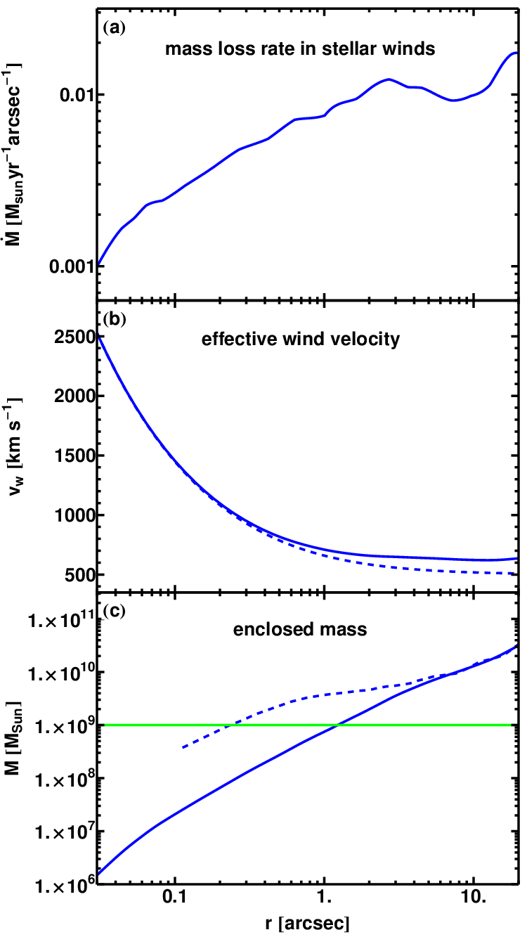
A direct by-product of measuring the velocity dispersion is the radial profile of the enclosed mass [46]. As the surface brightness profile is determined and deprojected, the mass-to-light ratio for the -band is computed at each radius. A constant value is reached far from the BH, despite the fact that the ratio varies close to the BH between different models of the velocity and the mass distributions. Neglecting any gradient in the stellar mass function, we assume a constant ratio for the enclosed stellar mass at any radius. Then we multiply the deprojected luminosity profile for the best-fitting D3 stellar dynamic model in Kormendy & Richstone [46] by the ratio and find the enclosed stellar mass. Direct inference of the enclosed stellar mass from the velocity dispersion is unreliable near the BH, when the BH mass is not precisely known. Setting a constant stellar allows to disentangle the BH mass from the stellar mass. In the bottom panel of Figure 2 we show the computed stellar enclosed mass (solid line) and the total enclosed mass calculated in Kormendy & Richstone [46] (dashed line).
II.2. Mass Injection
The most important feature of nuclear star clusters is the ability to inject matter, often in the form of stellar winds, to fuel the supermassive BHs. Many theoretical and observational studies of the matter injection rates and their relation to the observed quantities were conducted over the years (see Ho 37 for a review). The mass loss rate is found to be proportional to the stellar mass and to the stellar luminosity. The proportionality coefficients depend on the stellar population age . The correlation with stellar mass based on the stellar evolution models is summarized in Jungwiert et al. [43]. Their proposed formula reads
| (1) |
for solar stellar metallicity. Here is the initial stellar mass and Myr. We estimate the stellar age in the nucleus of NGC3115 with the stellar evolution code EzGal [54]. We run the simple stellar population models of Bruzual & Charlot [10] and Conroy et al. [15], Conroy & Gunn [14] for solar metallicity and reach the observed ratio for the age Gyr indicative of an old stellar population. At that age the stellar mass is [43] and the stellar mass loss rate is . We also discuss the gas and the stellar metallicities in Section II.5 below.
Another method to determine the stellar mass loss rate is from the correlation with the source luminosity. The mass loss rate is proportional to the -band luminosity as
| (2) |
for an old stellar population Faber & Gallagher [22], Padovani & Matteucci [67]. The normalization coefficient is known to within a factor of [37]. A similar relation exists between the and the -band luminosity [11, 4]. The normalizations determined by the formulas (1) and (2) agree for NGC3115 to within a factor of . These formulas are equivalent for a constant adopted ratio, and we use the latter one for convenience. We compute the profile of from the deprojected -band luminosity given by the best-fitting model D3 in Kormendy & Richstone [46].
We present the resultant mass loss rate in the top panel of Figure 2. While the mass loss rate per unit volume sharply rises towards the center, the depicted contribution per unit radius drops inwards. The area under the curve is the total mass injection rate. For the modeling of gas dynamics we normalize the mass loss rate by a radius-independent free parameter on the order unity .
II.3. Energy Injection
Several heating mechanisms with comparable power inputs operate in nuclear star clusters. First, when the mass loss is accomplished via stellar winds, those winds deposit their kinetic energy into the medium. The collisions of winds turn that kinetic energy into heat. Nuclear star clusters with young stellar populations, such as the one in our Galactic Center, produce winds with high velocities up to from Wolf-Rayet and other young stars [16]. However, old stellar populations mostly shed matter and produce winds from asymptotic giant branch (AGB) stars [91, 41, 31] with a correspondent wind velocity under [44, 56, 51, 50]. We use the terms ”stellar winds” and ”mass lost by stars” interchangeably, while having in mind that AGB stars shed mass also via planetary nebulae.
The mass-shedding stars move in a combined gravitational field of the BH and the enclosed stellar mass. The velocity of the relative stellar motions is on the order of the stellar velocity dispersion , which is in the NGC3115 nucleus [46]. Then the relative stellar motions introduce much more energy than the motions of matter with respect to the injecting stars [35], and the latter is ignored. For the purpose of the gas dynamical modeling we use the effective stellar wind velocity
| (3) |
given by the Keplerian velocity in the combined gravitational potential. Here is the BH gravitational radius.
Another important energy source are supernovae explosions. According to Mannucci et al. [55] the supernova rate in S0 galaxies (like NGC3115) is . Supernovae Type Ia occur in such galaxies more frequently than other kinds due to the large stellar population age. Each supernova is typically assumed to inject erg of useful energy [7] into the gas, while the typical ejecta mass is for the Type Ia [66]. Then the specific mass injection rate is . The specific mass injection rate in stellar winds is , so that supernovae inject a negligible amount of mass. The specific energy injection rate in stellar winds is for a typical velocity . The specific energy injection rate in supernovae is . The supernovae inject more energy than provided by stellar winds.
An important question is whether the energy injection by supernovae may be averaged over the characteristic gas flow timescale. Since a mass of about resides at the Bondi radius, one supernova should happen there every yrs. However, the sound crossing time is yrs. Then about supernovae happen before the system reacts, so we treat the energy injection from the supernovae on average. A more detailed a posteriori justification is given in Section VI.
Some energy is contributed into the feeding region by accreting objects such as low-mass X-ray binaries (LMXBs). We estimate the mechanical energy output of the accreting objects by equating it to their X-ray luminosity , which is a natural assumption for the most powerful high efficiency systems. Knowing that photons came from the LMXBs over Ms Chandra observation, we estimate their X-ray luminosity to be . Then the mechanical luminosity per unit mass is for a stellar mass of , which is an order of magnitude lower than the energy injection rate in supernovae or stellar winds. We neglect the energy contribution of the LMXBs.
In sum, the two dominant energy contributors are supernovae and colliding stellar winds. The specific energy injection rate is constant for the supernovae and is a strong function of radius for the colliding stellar winds. The supernova heating power is equivalent to the power of the colliding stellar winds with a velocity , which we call an effective supernova wind velocity. We combine the energy inputs into a total effective wind velocity as
| (4) |
In the middle panel of Figure 2 we plot for the fiducial (solid line) and for the same effective supernova contribution, but for the zero enclosed stellar mass (dashed line). In the modeling we leave the effective supernova wind velocity to be a free parameter, but check the best-fitting value of for consistency.
II.4. Angular Momentum Injection
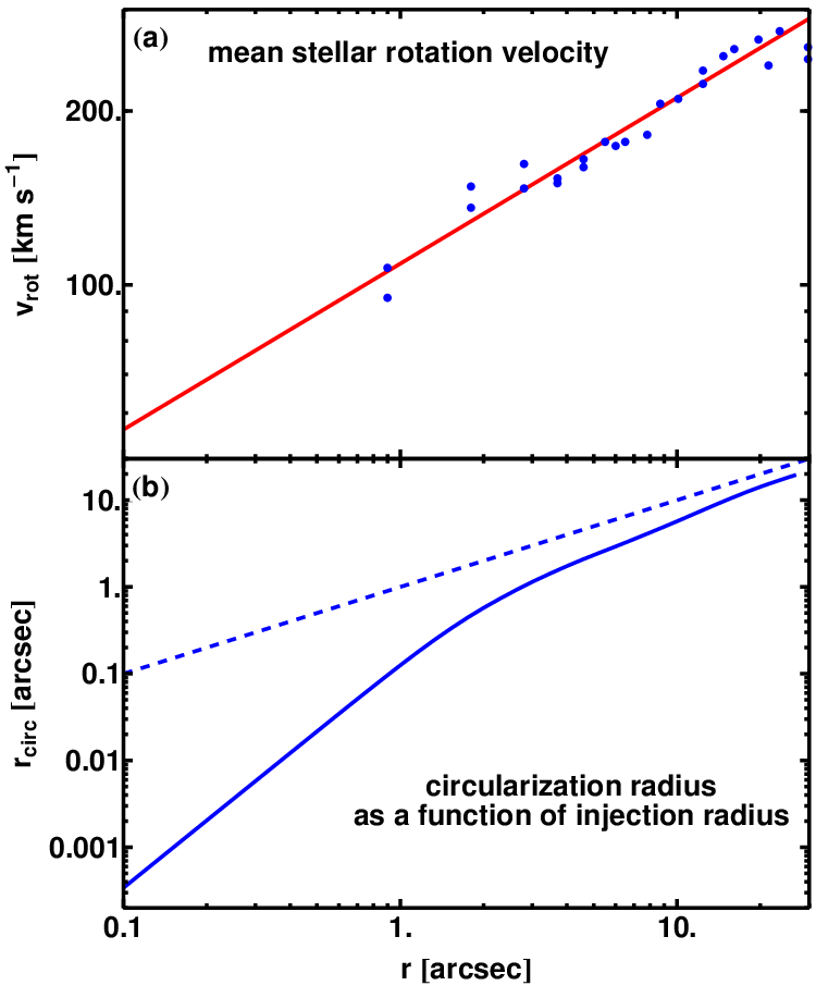
The NGC3115 nuclear star cluster possesses a non-zero mean rotation. In their paper Kormendy & Richstone [46] report the velocity profiles along the semi-major and semi-minor axes of the galaxy, which is viewed almost edge-on. The mean rotation is absent along the semi-minor axis, while the mean angular velocity measured along the semi-major axes reaches more than . In the top panel of Figure 3 we show the radial profile of the mean rotational velocity from Kormendy & Richstone [46]. We fit the data points with the power-law
| (5) |
which quickly approaches zero at a small radius. In the bottom panel of Figure 3 we show the circularization radius as a function of the injection radius (solid line) given as a solution of the equation
| (6) |
where the Keplerian velocity is computed in the joint gravitational potential. The dashed line given by the equation represents the injection with the Keplerian angular velocity . The presented radial dependence of the angular velocity qualitatively agrees with the transition to a rotationally supported galactic disk at a large radius and with the transition to purely random stellar motions at a small radius.
II.5. Gas Metallicity
It is difficult to determine the gas metallicity. The stars in the NGC3115 off-nuclear star clusters have sub-solar metallicity close to the center [3]. However, the stellar metallicity might not be a good proxy for the gas metallicity [88]. The gas metallicity is higher, since only the evolved stars with a large fraction of the heavy elements eject the substantial amounts of mass. Still, the stellar mass loss rate does not strongly depend on the stellar metallicity of AGB stars [57, 94]. Since the sound crossing time of the feeding region is only about yrs, the gas metallicity reflects the metallicity of the recently ejected mass.
While the metallicity of the hot gas in NGC3115 cannot be easily measured [96], the metallicity of the cooler gas is measured in many other galactic nuclei to be solar or super-solar [87, 34]. Relatively few examples exist with sub-solar gas metallicity [32]. Super-solar metallicity is also favored for the cool absorbing gas near Sgr A* in our Galactic Center [93]. With the absence of a better estimate we fix the gas metallicity in NGC3115 at the solar value . This approximation is not restrictive. As we discuss in Wong et al. [96], the gas metallicity is strongly degenerate with the density normalization. Since most of the X-rays are emitted in the metal lines, the gas density is inversely proportional to the assumed gas metallicity to preserve the constant density of metals.
III. GAS DYNAMICS
In Section II we characterized the gas injected into the BH feeding region. In this section we elaborate on the physical laws, which govern the gas dynamics. We first describe the distinct effects and then present a full set of radial equations.
III.1. Physical Effects
III.1.1 Conduction and Small-scale Feedback
Since the early introduction of ADAFs [9, 65], several effects were shown to break the advective nature of the hot radiatively inefficient accretion flows and result in a shallow density profile with , while for ADAFs. The flow is not advective, when the energy from the hotter inner flow is deposited into the cooler outer flow, which leads to a super-virial gas temperature. It immediately follows from the pressure balance equation
| (7) |
that in the absence of the source terms that a higher temperature leads to a shallower density slope .
We employ the term “small-scale feedback” for such energy transfer from the inner flow to the outer flow in an analogy with large-scale feedback, when the central AGN influences the entire galaxy [6, 19, 82]. The two main small-scale feedback processes are convection and conduction. Convection was shown to be important in collisional flows [63, 71]. Electron heat conduction appears to dominate convection in collisionless flows [79]. No heat is transferred via conduction across magnetic field lines, but the effective conductivity is still high in the turbulent flows as proposed theoretically [64] and confirmed with numerical simulations [68]. The action of conduction helps to explain the shallow density slope of the Sgr A* accretion flow [42, 79].
Outflows may lead to the shallow density profile as well [100]. However, it might be non-trivial to disentangle outflows from small-scale feedback. The simulations by Yuan et al. [101], Yuan et al. [99] showed both outflows above and below the midplane and convection in the equatorial plane. Small-scale feedback may help to launch the outflows. When convection or conduction transports energy outwards near the equatorial plane, outflows are more easily launched above and below the midplane facilitated by the higher gas temperature. Such a mechanism is distinct from ADIOS [8], which is based on outflows in the absence of small-scale feedback. Modeling the flow in one dimension, we do not distinguish between small-scale feedback and outflows. For the effective combined action of these effects we choose, following Shcherbakov & Baganoff [79], unsaturated conduction with the flux proportional to the temperature gradient with collisionless conductivity
| (8) |
The outer flow in NGC3115 is marginally collisional with a mean free path at the Bondi radius. However, as we show below, heat conduction effect is subdominant in the feeding region. The mean free path becomes equal to the radius at arcsec, where conduction becomes dynamically important. Thus, the solutions computed with high conductivity are physical, and we employ conductivity given by the formula (8) at any radius. The prescriptions with a lower conductivity in the outer flow reduce the stability of the numerical algorithm, and are avoided. To test the importance of small-scale feedback, we compute the flow models with and without conduction.
III.1.2 Gravitational Pull by the Enclosed Stellar Mass
The accretion flows governed by the BH gravity often smoothly connect to the galactic flows governed by the gravity of the enclosed mass [72]. According to Figure 2, the enclosed stellar mass in the NGC3115 nucleus exceeds the BH mass at about arcsec, which is less than the Bondi radius . Then, unlike in the Bondi model, constant temperature and constant density are not expected outside of . Outflows need more energy to escape the additional gravitational pull. The gas not bound to the BH may appear bound to the surrounding stellar mass.
III.1.3 Cooling
Cooling is another effect important for AGN feeding. Cool gas readily rushes onto the BH, as it does not have enough pressure to counteract the gravity. An inverted shape of the cooling curve supports a runaway catastrophe, as the gas loses energy slowly at K, but quickly at K [89]. The cooling power is proportional to the density squared , and the cooling timescale is inversely proportional to the density . Then this effect is less pronounced in low density systems such as the LLAGNs.
Cooling may influence the accretion in our Galactic Center. The marginal importance of cooling is indicated by Drappeau et al. [20] close to the plunging region of Sgr A*. Some models of Sgr A* show runaway cooling in the feeding region [17], while more realistic models exhibit milder temperature drops [16]. A setup very similar to NGC3115 was chosen by Gaspari et al. [26] for their numerical simulations of accretion flows. They find only a slight temperature reduction for the low density gas observed in the NGC3115 nucleus. Nevertheless, we include the effect of cooling in the dynamical modeling. We employ the CIE cooling curve from Sutherland & Dopita [89] and ignore the effects of clumping and spatial inhomogeneity.
III.1.4 Coupling of Ions and Electrons
The thermalization time of a particle distribution in hot tenuous gas is much shorter than the energy exchange time between the electrons and the ions via Coulomb collisions [81]. We follow the standard practice and consider thermal ions and thermal electrons with temperatures and , respectively. In addition to Coulomb collisions, relatively strong collisionless effects operate at high temperature [77]. However, we only consider Coulomb collisions in the modeling in the absence of a widely accepted prescription for collisionless coupling.
III.2. Dynamical equations
Following Shcherbakov & Baganoff [79], we solve the system of equations on the electron temperature , the ion temperature , the electron number density , and the gas radial velocity . The equations are modified from Shcherbakov & Baganoff [79], as we ignore the collisionless coupling of the species and the viscous conversion of the gravitational energy into thermal energy. The latter is justified, because, as we show in Section V, the stagnation point in the best-fitting solutions is at arcsec. Then the flow circularization radius lies within arcsec, and the viscous energy production is absent in the observed outer flow. The thermal energy production via the dissipation of the magnetic field is similarly unimportant till well within the stagnation point [78]. Two more modifications are the inclusion of cooling and the inclusion of the galactic gravitational potential. We present the full system of the dynamical equations here.
The mass balance equation is
| (9) |
where is the average atomic mass per electron for the assumed solar metallicity. The ratio of the number of ions to the number of electrons is . We consider the fully ionized species with the relative element abundances given by wilm table [95] 11 1 Note, that and slightly deviate from those in Shcherbakov & Baganoff [79] due to their use of a different abundance table.. We define the mass source function , such that the mass injection rate plotted in Figure 2 is . We normalize by the dimensionless number . We define the effective isothermal sound speeds
| (10) |
Then the Euler equation reads
| (11) |
where is the Lagrangian derivative.
The relativistic energy exchange rate per unit volume between the electrons and ions via Coulomb collisions is [86, 65]
| (12) | |||||
| (13) |
where is the modified Bessel function, the Coulomb logarithm is about , and the dimensionless electron and ion temperatures are
| (14) |
The rate simplifies to
| (15) | |||||
| (16) |
in a non-relativistic case.
The energy equations employ the relativistic electron energy
| (17) |
and the CIE cooling power [89]
| (18) |
for the cooling rate . Then the electron energy balance equation is
| (19) |
where the effective wind velocity is given by the formula (4). The ion energy balance is
| (20) |
While Shcherbakov & Baganoff [79] enhanced the rate of Coulomb collisions to enforce the temperature equality in the feeding region, we employ the normal rate of Coulomb collisions.
III.3. Free Parameters and Boundary Conditions
We search for the stationary solutions of the system of equations (9,11,19, and 20) with the shooting method. The system has four free parameters: the BH mass , the normalization of the mass source function , the effective supernova wind velocity , and the stagnation point radius . Multiple solutions exist, however, for each set of these parameters. We identify a set of the natural boundary conditions and the constraints, which leads to a unique solution. These are
- 1.
equal electron and ion temperatures at a large radius,
- 2.
the presence of a sonic point in the accretion flow and the absence of shocks,
- 3.
and the zero gradient of the electron temperature close to the BH .
The third condition is practically equivalent to the requirement of the mere existence of the solution down to the BH horizon. We also search for advective solutions of the same system of equations by setting the conductivity to zero. Only the first two conditions are imposed to find a unique advective solution.
IV. FITTING XVP DATA
Having presented the dynamical model, in this section we discuss the X-ray data and outline the computations of the simulated spectra and the fitting technique. Previous source modeling relied on earlier Chandra observations with ks total exposure [97]. New observations with a combined exposure Ms were performed in 2012 within Chandra XVP. The new data and their model-independent analysis are presented in a companion paper Wong et al. [96]. The deep X-ray observations of the NGC3115 nucleus reveal the extended source centered on the BH, which consists of the gas and unresolved point sources.
IV.1. CIE or Non-equilibrium Ionization?
The gas temperature is about keV, so that the emission is dominated by metal lines at keV [97]. The line emission power is influenced by the gas ionization state. The collisions of the stellar winds and the shock waves from supernovae lead to the episodes of instantaneous heating. The heating episodes throw the gas into a non-equilibrium ionization (NEI) state. The CIE is restored after a large number of particle collisions. The number of collisions is quantified by the ionization timescale, a product of the density by the time . We estimate at a arcsec radius, where the density is [97]. The region has a sound crossing time yrs, during which about supernovae explode. Then the same portion of gas is shocked every yrs. The ionization timescale between shocks is , for which the flow might not attain full ionization equilibrium [83]. However, as we show below, cooling is relatively weak in the best-fitting flow solutions. A passage of a single shock might not substantially change the gas temperature, so that the effective ionization timescale is much larger, and the CIE assumption is justified. For the gas radiation we use the CIE model apec based on ATOMDB 2.0.1 [23] as implemented in XSPEC 12.8 [2]. The NEI effects are to be explored in future work.
IV.2. Optical Depth Effects
The optical depth also influences the line emission power. Here we show that the X-ray radiation in the NGC3115 nucleus is optically thin to both absorption and resonant scattering. Let us make a strong assumption that all the X-ray luminosity is concentrated in a single line. We set the line energy at the peak of the observed gas spectrum keV. The temperature in the region is keV [97], so that the line is subject to thermal broadening by . Let us now compare the blackbody luminosity in this line with the total observed luminosity to estimate the efficiency of absorption. The blackbody source function is
| (21) |
Then the blackbody line luminosity is
| (22) |
emitted by a sphere with a radius arcsec. This is about orders of magnitude above the observed luminosity.
Resonant scattering may have a larger effect as it is found to change the surface brightness profiles of elliptical galaxies [80]. Shigeyama [80] estimate the emission averaged optical depth to be around over the scattering column density for the relevant gas temperature. The scattering column density to the center of NGC3115 is about and the correspondent optical depth is . Thus, the gas emission is optically thin to both absorption and scattering.
IV.3. Point sources
The contamination by the point sources complicates the modeling of the gas emission. We subtract the brightest isolated objects, but source confusion precludes the reliable subtraction at radii arcsec. The weaker and confused point sources contribute to the extended emission. A reliable spectral model is the key to discriminate such emission from the gas emission.
LMXBs comprise most of the resolved and some of the unresolved point source emission. The combined spectrum of the resolved LMXBs is an absorbed power-law with index [97], and we use the same index to model the unresolved LMXBs. The nuclear LMXB luminosity is proportional to the stellar mass [28, 59]. However, as the nuclear luminosity in NGC3115 is dominated by a few bright sources, the Poisson noise in the proportionality coefficient is large. We leave the normalization of the LMXB luminosity to be a free parameter.
Cataclysmic variables and coronally active stars contribute to the diffuse X-ray emission as the so-called CV/AB component [74, 73]. Following Wong et al. [96] we model the CV/AB contribution as an absorbed sum of a power-law with an index and a thermal component with keV. The total CV/AB luminosity is computed from the relation and the surface brightness is taken to be proportional to the optical surface brightness. Each CV/AB source is relatively weak, so that many sources contribute to the emission, and Poisson noise is insignificant. The CV/ABs is a sub-dominant component in the inner flow [96].
IV.4. Point Spread Function
The Chandra observations probe the inner several arcseconds around the supermassive BH in NGC3115. Since spatial variations are expected on the scale of arcsec, the results of such observations are affected by photon redistribution due to the finite size of the point spread function (PSF). An implementation of the resultant PSF spreading is generally available in XSPEC as the mixing models, yet no such model exists for the Chandra PSF. We implement the PSF spreading in Mathematica 9 and perform consistency checks. For simplicity, we adopt an energy-independent Gaussian PSF with width , which fits the core of the surface brightness profile of a nearby point source.
IV.5. Procedure
There are many ways to compare the simulated emission from the accretion flow model to the observations. For example, Shcherbakov & Baganoff [79] compared the energy-integrated profiles of the surface brightness. This approach introduces a degeneracy between the temperature and the density: the high temperature low density model produces the same surface brightness as the low temperature high density model. The degeneracy may be broken with the use of the spectrum. Fitting the radius-integrated spectrum [93] one obtains the relative contributions of gas at the different temperatures with little information about the spatial distribution. Thus, we maintain both the spectral and the spatial information, while comparing the simulated emission to the data.
Following Wong et al. [96] we divide the BH feeding region into circular rings centered on the BH. In this paper we limit ourselves to an outer radius of arcsec, which is far outside of . We define rings with the projected radii in the ranges arcsec, arcsec, arcsec, arcsec, arcsec, arcsec, and arcsec. The spectrum of each ring is extracted and grouped with a minimum of photons per bin for a total of bins over the rings. Having defined the observed spectra, we calculate the simulated spectra and compute the chi-square statistic.
The simulated spectrum in each ring is the sum of the fixed CV/AB contribution, the fixed background, the power-law LMXB component with a free normalization, and the gas component. Since the background dominates at high energies, we set the high energy limit at keV. We set the low energy limit at keV as the lowest bin energy for the grouped observed spectrum.
The gas properties are defined by the computed profiles of the temperatures and and the electron density for the radius from arcsec to arcsec. We set the density to zero outside of this radial range. We calculate the simulated spectra fully self-consistently. We divide the flow into many spherical shells and compute the contributions of each shell into the projected rings, while taking into account the PSF spreading. We find a joint as a sum over all rings. We perform the steepest descent search for a minimum of over the set of the model parameters. We explore the BH masses in the range motivated by the dynamical modeling of the stellar motions [48, 21]. We do not restrict the other three free parameters , , and . We find the best-fitting conductive and advective solutions.
V. RADIAL INFLOW-OUTFLOW SOLUTIONS
V.1. Solutions with Conduction

The dynamical structure of the best-fitting solution with conduction is shown in Figure 4. This solution is achieved at the lower BH mass boundary for the mass loss rate normalization , the effective supernova wind velocity , and the stagnation point radius arcsec. It reaches for and has an accretion rate . This accretion rate is a factor of lower than Bondi accretion rate [97]. However, the correspondent accretion power is still about orders of magnitude larger than the observed jet radio power. The density (shown in the top panel) behaves approximately as over the large range of the radius. The density does not flatten out outside of the Bondi radius. The electron temperature is higher than the ion temperature due to heat conduction, which primarily influences the electrons. The ion temperature is approximately virial at all radii, which corresponds to in the inner flow. The slope of is relatively flat in the outer flow, where the enclosed mass increases with radius as , so that . The gas inflow velocity (shown in the bottom panel) exceeds the sound speed at a relatively large radius . This is a consequence of the rising electron heat capacity [78] and the absence of super-virial heating. The outflow velocity is much below the sound speed in the outer flow, so that the outflow is subsonic. The determined stagnation point radius corresponds to the circularization radius of according to Figure 3. Relatively little X-ray emission originates within this radius in a non-cooling accretion flow.

In the middle panel of Figure 4 we depict the confidence range of the temperature (green/light area) in the ”single-T apec per annulus” best-fitting model presented in Wong et al. [96]. In this model the observed spectrum in each annulus is fitted independently with a single-temperature apec component instead of drawing the gas temperatures from a smooth radial profile. The point source and the background contributions are computed the same way in both kinds of models. The temperature in the ”single-T apec per annulus” best-fitting model agrees with the temperature in the best-fitting conductive solution at large radii arcsec, but deviates down in the inner flow.
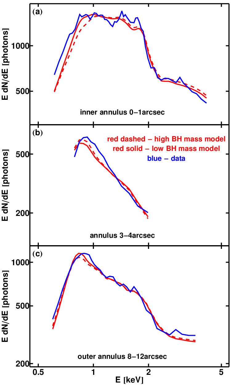
As we show in Figure 5 the ”single-T apec per annulus” model reaches lower with the more uniform residuals . The best-fitting solution with conduction underpredicts the observed soft flux as evident from the systematic trend at the lowest energies in the top panel. In sum, while our solution could be improved with the lower temperature in the inner flow, it already provides an acceptable fit to the data with . The reasons for this underprediction are explored in Wong et al. [96], the main hypothesis being the presence of an inner soft component, which appears to be extended. This soft component could either be a cool diffuse gas or a distinct population of point sources. Wong et al. [96] develop a two-component gas model and obtain a temperature profile of the hotter component, which agrees with the best-fitting profile of the electron temperature. The data and the model are shown for selected annuli in Figure 6 for low BH mass () and high BH mass () best-fitting solutions with conduction. Lack of strong soft emission is evident in both the inner and the outer annuli for both BH masses. Substantial non-thermal emission convolved with Chandra response function is responsible for keV bump in the outer annuli, while the extended bump in keV energy range in the inner annuli is mainly emitted by the hot inner accretion flow. The annuli with projected radii within arcsec exhibit relatively soft spectrum, while the models are substantially harder. As indicated by ”single-T apec per annulus” model, a hotter thermal plasma provides a better fit to that spectrum. Since the galactic gravitational potential dominates the BH potential at arcsec distance, then the differences between the low BH mass and the high BH mass models are the most evident in the inner annulus. The high BH mass model has a higher virial temperature. This leads to further underprediction of the soft flux emitted by the inner accretion flow, so that high BH mass model provides a worse fit to the data.
V.2. Advective Solutions and Comparison

We explore not only the solutions with conduction, but also the advective solutions, where the conductivity is set to zero. The comparison between these cases helps to explore the role of conduction. In Figure 7 we show the dynamical quantities for the best-fitting solution without conduction (dashed) and for the best-fitting solution with conduction (solid). The best fit among the advective solutions is also achieved at the lower BH mass boundary . The correspondent values of the free parameters are , , and arcsec. This solution reaches and has an accretion rate . The values of the free parameters are similar in the best-fitting conductive and advective solutions, except the stagnation point is much further out in the advective solution and the accretion rate is much higher. This difference is a natural consequence of conduction. The density profiles in both best-fitting solutions asymptote to the steep Bondi profile in the inner flow. However, the inner flow density and the accretion rate are a factor of higher in the advective solution. This factor may be even larger, when super-virial heating is included [42, 79]. As super-virial heating is likely important in the inner flow, the computed accretion rate is an upper limit on the rate of mass crossing the event horizon. The electron temperature in the advective solution is lower than the ion temperature due to cooling in the outer flow and the higher electron heat capacity in the inner flow. The solution with conduction has a factor of lower inner ion temperature. The energetics of the outer flow are mainly determined by the mass injection and the energy injection, so that the properties of the outer flow are similar between the two best-fitting solutions.
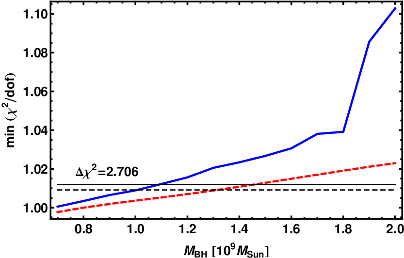
One of the most important results of the presented model fitting is the BH mass. In Figure 8 we show the reduced as a function of the BH mass for both the best-fitting advective models (red/dashed line) and the best-fitting models with conduction (blue/solid line). Both types of models show a clear rising trend with the BH mass in agreement with Figure 6 and discussion of the spectral features therein. The confidence range limits the BH mass to below for the conductive models and to below for the advective models in agreement with the latest BH mass estimates [21]. However, the adopted modeling has many caveats, which should be carefully examined before the firm conclusions are drawn about the BH mass. Here we demonstrate that it is possible to discriminate between the models with the different BH masses by fitting the X-ray data. We discuss the caveats of the modeling in the next section.
VI. DISCUSSION AND CONCLUSIONS
VI.1. Summary of Results
In the paper we present the modeling of the X-ray data from Ms Chandra XVP observation of the NGC3115 center. We connect the properties of the nuclear star cluster known from optical observations to the properties of the X-ray emitting hot gas. We construct the radial inflow-outflow dynamical models, which include many physical effects: the matter and the energy injection by stellar winds and supernovae, conduction, the additional gravitational pull by the enclosed mass, cooling, and Coulomb collisions. We simulate the X-ray emission from the models and fit the set of the X-ray spectra in concentric annuli around the BH. We find best-fitting models with an acceptable . The proposed models are sensitive to the BH mass and favor low values . We estimate the normalization of the mass source function to be , which is somewhat smaller than the expected value . We discuss below the reasons for the deviation of from unity distinct from the uncertainties in the mass loss rate. The best-fitting effective supernova wind velocity is , which corresponds to the rate of the supernova explosions for the fiducial energy release per event. This estimated event rate is consistent with the observed event rate in S0 galaxies like NGC3115 [55]. The stagnation point is at arcsec for the best-fitting solution with conduction and at arcsec for the best-fitting advective solution. Therefore most of the ”accretion flow” seen by Chandra is outflowing from the region, while the stagnation radius scale is barely resolved. We find that the best-fitting conductive and advective solutions behave similarly in the outer flow, yet the advective solution has the higher density and the lower electron temperature in the inner flow.
It is instructive to compare the relative strengths of the various effects by computing the correspondent timescales. In Figure 9 we plot the timescales in the feeding region. The sound crossing time (blue/upper thick solid line)
| (23) |
is about the free fall time (green/lower thick solid line)
| (24) |
so that the gas temperature is close to virial at any radius. We also plot the cooling time (brown/short-dashed line)
| (25) |
the conductive heating time (magenta/long-dashed line)
| (26) |
is the divergence of the conduction heat flux, and the mass injection time (red/dot-dashed line)
| (27) |
The cooling timescale is about times the free-fall timescale , so that cooling is expected to be unimportant in the modeled hot-phase gas in the non-rotating flow [26]. The mass injection time is much larger than either or , which indicates a relatively slow radial gas velocity . The conductive heating time is very large outside of arcsec, so that the solutions with and without conduction behave similarly in the outer flow. This timescale gets comparable to the injection time inside of arcsec, which suggests the importance of conduction at those radial scales. The comparison of timescales also helps to establish the self-consistency of the model. The time between consecutive supernova explosions (black/thin solid line)
| (28) |
becomes longer than the sound crossing time at arcsec. Thus, the energy injection from the supernovae cannot be treated on average in the inner flow. However, this mechanism is subdominant at arcsec as evident from the middle panel in Figure 2: the collisions of stellar winds supply most of the energy in the inner flow. The inner accretion flow experiences relatively weak disturbances from supernova explosions, which are washed away on the dynamical timescale. Then the average energy injection rate is well-defined at any radius.

VI.2. What Does the Density Slope Mean?
The modeling of the resolved X-ray emission gives the gas density slope. We find the shallow density profile with across a large range of scales in the NGC3115 nucleus. As briefly discussed in Section III.1, the shallow density profile commonly occurs in CDAFs [71, 63], in the accretion flows with conduction [42, 79], and in the accretion flows with the outflows above and below the midplane [8, 100, 101]. However, there are other reasons to have near the Bondi radius in the hot gas flows. Let us elaborate on the effects either directly responsible for the shallow density profile or calling for the extension of the aforementioned explanations.
First, we examine the original Bondi solution as computed by Bondi [9]. Their curve II in Figure 5 shows the relevant case of an adiabatic transonic inflow for the adiabatic index . In this solution the density slope is a function of radius and changes from at to at . The steep asymptotic behavior is achieved only very deep inside the Bondi sphere. The Bondi flow has at a tenth of the Bondi radius , which corresponds to their dimensionless radius . The slope at a radius arcsec probed by the Chandra satellite in NGC3115 is expected to be even in a fully advection-dominated Bondi-like flow.
Second, we model the material in NGC3115 to outflow from the stagnation point at arcsec. However, when the mean radial velocity is much smaller than the sound speed , then the small-scale feedback and the outflows have the same power for both positive and negative . The pressure balance is practically hydrostatic for small and is given by the equation (7). Then small-scale feedback and outflows make the density profile shallow in both the inflow region and the outflow region. However, the density in the outflow asymptotes to , if the radial velocity is large, while the density is constant in the Bondi inflow. Models with large outflow velocity are disfavored for NGC3115, while being viable for Sgr A* [70].
Third, continuous mass injection modifies the mass conservation law, so that . Mass injection is the dominant term in the density balance at radii arcsec in the best-fitting solution with conduction. Then mass conservation law is inapplicable in the feeding region of NGC3115 near the Bondi radius . The density slope in the outer flow is influenced by the matter source term.
Fourth, the region near and outside of the Bondi radius is influenced by the gravity of the enclosed mass. The correspondent gravitational potential does not flatten, but increases with radius. Then the gas outflow velocity stays small and the asymptotic outflow behavior is not reached. The virial temperature is much higher in the outer gas, when the enclosed mass from the nuclear star cluster is included. As the gas temperature closely follows the virial temperature, the change in the virial temperature profile influences the density profile. The density profile is commonly observed in the hot flows outside of the Bondi radius [1, 97], where the galactic gravitational potential matters.
The interplay of these four processes and effects determines the gas density profiles in the LLAGNs. Despite the slope approximates the density profile in NGC3115 over a large radial range, the local slope at a given often substantially deviates from . The absence of a single behavior over a large dynamic range demotivates us from isolating the self-similar solutions.
VI.3. Limitations of the Dynamical Model
Despite being able to fit the data, the presented models are not fully self-consistent. Let us examine the drawbacks and the limitations of the models and outline a more self-consistent treatment.
VI.3.1 Inhomogeneous Medium
The observational studies of Sgr A* suggest inhomogeneous gas near the Bondi radius [5, 62, 93]. Regions with vastly different temperatures readily co-exist, while the Chandra satellite only sees the hot dense counterparts with temperature keV. Nevertheless, the observed gas temperature keV in NGC3115 agrees well with the virial temperature , and the observed density is reproduced with the normalization of the mass source function on the order unity. Then the hot gas likely constitutes the dominant gas component.
The filling factor of this hot component may still be below unity . In this case the mean density required to reproduce the observations is lower. More generally, gas with lower mean density reproduces the observations, when substantial density fluctuations are present. Since the emissivity is proportional to , then thinking of the best-fitting density as the root-mean-squared quantity effectively takes the inhomogeneities into account.
VI.3.2 Non-stationary Solutions
A wide range of non-stationary behaviors, such as oscillation cycles, may occur in accretion flows. The best-fitting energy of the outflowing gas is barely enough to escape the gravitational potential of the enclosed mass. The temperatures in the best-fitting ”single-T apec per annulus” model are even lower [96], so that the gas may be unable to escape. When the gas inflow rate is limited and the outflow rate is zero, matter gradually accumulates in the BH feeding region owing to stellar mass loss.
The accumulation of matter leads to a higher density, and the gas eventually cools. Cooling leads to a higher accretion rate, since the cooler gas does not counteract the gravity and since accretion is not inhibited by small-scale feedback, when the temperature is sub-virial. The burst of accretion empties the feeding region. The accretion rate drops after the burst, and then a new phase of matter accumulation begins. The accumulation phase of such accumulation-accretion cycles might reproduce the current state of NGC3115. This possibility is to be explored with future time-dependent numerical simulations.
VI.3.3 Angular Momentum Transport
We did not explicitly treat angular momentum transport, which is partially justified a posteriori. We find a relatively small circularization radius arcsec in the best-fitting solutions. The accretion flow at arcsec probed with Chandra might not feel the difference with an explicit treatment of the inner flow circularization. The sonic point in the circularized flow is closer to the BH [69], and the influence of conduction is expected to be stronger. Then the shallow density profile is expected to continue down to several . Having defined the injection of the angular momentum, we leave angular momentum transport and the inner flow connection for future work.
VI.4. Limitations of the Radial Solutions
The presented modeling is performed under the strong approximation of one dimension. The resultant treatment of gravitational forces is approximate and gas motions are restricted.
We compute the enclosed mass profile based on the surface brightness along the semi-major axis assuming zero ellipticity of the stellar distribution. However, Kormendy & Richstone [46] report an ellipticity of at the Bondi radius. Since the ellipticity varies with radius and the gravitational force is not trivially determined for a non-spherical mass distribution, we do not improve in this work upon the zero ellipticity approximation.
The gravitational force is generally lower in the case of non-zero ellipticity. To test the effect of a lower gravitational force we search for a best-fitting solution with a smaller enclosed mass and a fixed BH mass . We find the best-fitting advective solution with a higher normalization of the mass source function compared to for the of the enclosed mass. The resultant normalization is much closer to unity, while varies little across the best-fitting solutions with different . The effective supernova wind velocity is for the of the enclosed mass compared to for the . The correspondent change of the stagnation radius is from arcsec to arcsec. The reduced chi-squared shows a small improvement by .
The gas in the one-dimensional solution is restricted to either inflow or outflow radially. More complex patterns may occur in two dimensions, such as inflow in the equatorial plane with outflow along the angular momentum axis. While typical density and temperature profiles in two-dimensional solutions may be similar to those in one-dimensional solutions [101, 75], more detailed fitting of the data with the two-dimensional solutions is warranted. The lower gravitational force facilitates the outflow along the angular momentum axis. This leads to an easier evacuation of the feeding region, so that the best-fitting two-dimensional solutions are expected to have a higher normalization of the mass loss rate. Finding the self-consistent two-dimensional solutions might require the numerical simulations, and the present manuscript provides a starting point for such work.
VII. Acknowledgements
The authors thank Sam Leitner, Alexey Vikhlinin, Tassos Fragos, Sergey Nayakshin, Kazimierz Borkowski, Feng Yuan, Ranjan Vasudevan, and Richard Mushotzky for stimulating discussions and the anonymous referee for useful suggestions. The work is supported by Chandra XVP grant GO2-13104X. RVS is supported by NASA Hubble Fellowship grant HST-HF-51298.01. RVS acknowledges hospitality of the Physics and Astronomy Department, University of North Carolina, Chapel Hill, where a part of the work was conducted.
References
- [1] Allen, S. W., Dunn, R. J. H., Fabian, A. C., Taylor, G. B., & Reynolds, C. S. 2006, MNRAS, 372, 21
- [2] Arnaud, K. A. 1996, in Astronomical Society of the Pacific Conference Series, Vol. 101, Astronomical Data Analysis Software and Systems V, ed. G. H. Jacoby & J. Barnes, 17
- [3] Arnold, J. A., Romanowsky, A. J., Brodie, J. P., Chomiuk, L., Spitler, L. R., Strader, J., Benson, A. J., & Forbes, D. A. 2011, ApJ, 736, L26
- [4] Athey, A., Bregman, J., Bregman, J., Temi, P., & Sauvage, M. 2002, ApJ, 571, 272
- [5] Baganoff, F. K., et al. 2003, ApJ, 591, 891
- [6] Begelman, M. C., & Nath, B. B. 2005, MNRAS, 361, 1387
- [7] Benson, A. J. 2010, Phys. Rep., 495, 33
- [8] Blandford, R. D., & Begelman, M. C. 1999, MNRAS, 303, L1
- [9] Bondi, H. 1952, MNRAS, 112, 195
- [10] Bruzual, G., & Charlot, S. 2003, MNRAS, 344, 1000
- [11] Ciotti, L., D’Ercole, A., Pellegrini, S., & Renzini, A. 1991, ApJ, 376, 380
- [12] Ciotti, L., & Ostriker, J. P. 2001, ApJ, 551, 131
- [13] —. 2007, ApJ, 665, 1038
- [14] Conroy, C., & Gunn, J. E. 2010, ApJ, 712, 833
- [15] Conroy, C., Gunn, J. E., & White, M. 2009, ApJ, 699, 486
- [16] Cuadra, J., Nayakshin, S., & Martins, F. 2008, MNRAS, 383, 458
- [17] Cuadra, J., Nayakshin, S., Springel, V., & Di Matteo, T. 2005, MNRAS, 360, L55
- [18] Czerny, B., Kunneriath, D., Karas, V., & Das, T. K. 2013, A&A, 555, A97
- [19] Di Matteo, T., Springel, V., & Hernquist, L. 2005, Nature, 433, 604
- [20] Drappeau, S., Dibi, S., Dexter, J., Markoff, S., & Fragile, P. C. 2013, MNRAS, 431, 2872
- [21] Emsellem, E., Dejonghe, H., & Bacon, R. 1999, MNRAS, 303, 495
- [22] Faber, S. M., & Gallagher, J. S. 1976, ApJ, 204, 365
- [23] Foster, A. R., Ji, L., Smith, R. K., & Brickhouse, N. S. 2012, ApJ, 756, 128
- [24] Freitag, M., & Benz, W. 2002, A&A, 394, 345
- [25] Garcia, M. R., et al. 2010, ApJ, 710, 755
- [26] Gaspari, M., Ruszkowski, M., & Oh, S. P. 2013, MNRAS, 432, 3401
- [27] Genzel, R., Eisenhauer, F., & Gillessen, S. 2010, Reviews of Modern Physics, 82, 3121
- [28] Gilfanov, M. 2004, MNRAS, 349, 146
- [29] Graham, A. W., & Spitler, L. R. 2009, MNRAS, 397, 2148
- [30] Greene, J. E., & Ho, L. C. 2007, ApJ, 667, 131
- [31] Groenewegen, M. A. T., et al. 2007, MNRAS, 376, 313
- [32] Groves, B. A., Heckman, T. M., & Kauffmann, G. 2006, MNRAS, 371, 1559
- [33] Guo, F., & Mathews, W. G. 2013, eprint arXiv:1305.2958
- [34] Hamann, F., Korista, K. T., Ferland, G. J., Warner, C., & Baldwin, J. 2002, ApJ, 564, 592
- [35] Hillel, S., & Soker, N. 2013, MNRAS, 430, 1970
- [36] Ho, L. C. 2008, Ann. Rev. Astron. Astr., 46, 475
- [37] —. 2009, ApJ, 699, 626
- [38] Holzer, T. E., & Axford, W. I. 1970, ARA&A, 8, 31
- [39] Hopkins, P. F., & Hernquist, L. 2006, ApJS, 166, 1
- [40] —. 2009, ApJ, 698, 1550
- [41] Hurley, J. R., Pols, O. R., & Tout, C. A. 2000, MNRAS, 315, 543
- [42] Johnson, B. M., & Quataert, E. 2007, ApJ, 660, 1273
- [43] Jungwiert, B., Combes, F., & Palouš, J. 2001, A&A, 376, 85
- [44] Knapp, G. R., Phillips, T. G., Leighton, R. B., Lo, K. Y., Wannier, P. G., Wootten, H. A., & Huggins, P. J. 1982, ApJ, 252, 616
- [45] Kormendy, J., & Gebhardt, K. 2001, in American Institute of Physics Conference Series, Vol. 586, 20th Texas Symposium on relativistic astrophysics, ed. J. C. Wheeler & H. Martel, 363–381
- [46] Kormendy, J., & Richstone, D. 1992, ApJ, 393, 559
- [47] —. 1995, Ann. Rev. Astron. Astr., 33, 581
- [48] Kormendy, J., et al. 1996, ApJ, 459, L57
- [49] Lamers, H. J. G. L. M., & Cassinelli, J. P. 1999, Introduction to Stellar Winds (Cambridge University Press)
- [50] Leitner, S. N., & Kravtsov, A. V. 2011, ApJ, 734, 48
- [51] Libert, Y., Gérard, E., Thum, C., Winters, J. M., Matthews, L. D., & Le Bertre, T. 2010, A&A, 510, A14
- [52] MacLeod, M., Guillochon, J., & Ramirez-Ruiz, E. 2012, ApJ, 757, 134
- [53] MacLeod, M., Ramirez-Ruiz, E., Grady, S., & Guillochon, J. 2013, eprint arXiv:1307.2900
- [54] Mancone, C. L., & Gonzalez, A. H. 2012, PASP, 124, 606
- [55] Mannucci, F., Della Valle, M., Panagia, N., Cappellaro, E., Cresci, G., Maiolino, R., Petrosian, A., & Turatto, M. 2005, A&A, 433, 807
- [56] Marengo, M. 2009, Publications of the Astronomical Society of Australia, 26, 365
- [57] Marigo, P., & Girardi, L. 2007, A&A, 469, 239
- [58] Mathews, W. G., & Brighenti, F. 2003, ARA&A, 41, 191
- [59] Miller, B., Gallo, E., Treu, T., & Woo, J.-H. 2012, ApJ, 747, 57
- [60] Milosavljević, M. 2004, ApJ, 605, L13
- [61] Milosavljević, M., Merritt, D., & Ho, L. C. 2006, ApJ, 652, 120
- [62] Muno, M. P., Baganoff, F. K., Brandt, W. N., Morris, M. R., & Starck, J.-L. 2008, ApJ, 673, 251
- [63] Narayan, R., Igumenshchev, I. V., & Abramowicz, M. A. 2000, ApJ, 539, 798
- [64] Narayan, R., & Medvedev, M. V. 2001, ApJ, 562, L129
- [65] Narayan, R., & Yi, I. 1995, ApJ, 452, 710
- [66] Nauenberg, M. 1972, ApJ, 175, 417
- [67] Padovani, P., & Matteucci, F. 1993, ApJ, 416, 26
- [68] Parrish, I. J., Quataert, E., & Sharma, P. 2010, ApJ, 712, L194
- [69] Popham, R., & Gammie, C. F. 1998, ApJ, 504, 419
- [70] Quataert, E. 2004, ApJ, 613, 322
- [71] Quataert, E., & Gruzinov, A. 2000, ApJ, 539, 809
- [72] Quataert, E., & Narayan, R. 2000, ApJ, 528, 236
- [73] Revnivtsev, M., Churazov, E., Sazonov, S., Forman, W., & Jones, C. 2008, A&A, 490, 37
- [74] Revnivtsev, M., Sazonov, S., Gilfanov, M., Churazov, E., & Sunyaev, R. 2006, A&A, 452, 169
- [75] Sadowski, A., Narayan, R., Penna, R., & Zhu, Y. 2013, eprint arXiv:1307.1143
- [76] Seth, A., Agüeros, M., Lee, D., & Basu-Zych, A. 2008, ApJ, 678, 116
- [77] Sharma, P., Quataert, E., Hammett, G. W., & Stone, J. M. 2007, ApJ, 667, 714
- [78] Shcherbakov, R. V. 2008, ApJS, 177, 493
- [79] Shcherbakov, R. V., & Baganoff, F. K. 2010, ApJ, 716, 504
- [80] Shigeyama, T. 1998, ApJ, 497, 587
- [81] Shkarofsky, I. P., Johnston, T. W., & Bachynski, M. P. 1966, The particle kinetics of plasma (London: Addison-Wesley Publishing Company)
- [82] Silk, J., & Nusser, A. 2010, ApJ, 725, 556
- [83] Smith, R. K., & Hughes, J. P. 2010, ApJ, 718, 583
- [84] Soria, R., Fabbiano, G., Graham, A. W., Baldi, A., Elvis, M., Jerjen, H., Pellegrini, S., & Siemiginowska, A. 2006a, ApJ, 640, 126
- [85] Soria, R., Graham, A. W., Fabbiano, G., Baldi, A., Elvis, M., Jerjen, H., Pellegrini, S., & Siemiginowska, A. 2006b, ApJ, 640, 143
- [86] Stepney, S., & Guilbert, P. W. 1983, MNRAS, 204, 1269
- [87] Storchi Bergmann, T., & Pastoriza, M. G. 1989, ApJ, 347, 195
- [88] Su, Y., & Irwin, J. A. 2013, ApJ, 766, 61
- [89] Sutherland, R. S., & Dopita, M. A. 1993, ApJS, 88, 253
- [90] Tonry, J. L., Dressler, A., Blakeslee, J. P., Ajhar, E. A., Fletcher, A. B., Luppino, G. A., Metzger, M. R., & Moore, C. B. 2001, ApJ, 546, 681
- [91] Vassiliadis, E., & Wood, P. R. 1993, ApJ, 413, 641
- [92] Volonteri, M., Dotti, M., Campbell, D., & Mateo, M. 2011, ApJ, 730, 145
- [93] Wang, Q. D., et al. 2013, Science, 341, 981
- [94] Weiss, A., & Ferguson, J. W. 2009, A&A, 508, 1343
- [95] Wilms, J., Allen, A., & McCray, R. 2000, ApJ, 542, 914
- [96] Wong, K.-W., Irwin, J. A., & Shcherbakov, R. V. 2013, ApJ in press, arXiv:1311.0868
- [97] Wong, K.-W., Irwin, J. A., Yukita, M., Million, E. T., Mathews, W. G., & Bregman, J. N. 2011, ApJ, 736, L23
- [98] Wrobel, J. M., & Nyland, K. 2012, AJ, 144, 160
- [99] Yuan, F., Bu, D., & Wu, M. 2012a, ApJ, 761, 130
- [100] Yuan, F., Quataert, E., & Narayan, R. 2003, ApJ, 598, 301
- [101] Yuan, F., Wu, M., & Bu, D. 2012b, ApJ, 761, 129