UCB-PTH-13/07
Black Holes or Firewalls: A Theory of Horizons
Yasunori Nomura, Jaime Varela, and Sean J. Weinberg
Berkeley Center for Theoretical Physics, Department of Physics,
University of California, Berkeley, CA 94720, USA
Theoretical Physics Group, Lawrence Berkeley National Laboratory, CA 94720, USA
We present a quantum theory of black hole (and other) horizons, in which the standard assumptions of complementarity are preserved without contradicting information theoretic considerations. After the scrambling time, the quantum mechanical structure of a black hole becomes that of an eternal black hole at the microscopic level. In particular, the stretched horizon degrees of freedom and the states entangled with them can be mapped into the near-horizon modes in the two exterior regions of an eternal black hole, whose mass is taken to be that of the evolving black hole at each moment. Salient features arising from this picture include: (i) the number of degrees of freedom needed to describe a black hole is , where is the area of the horizon; (ii) black hole states having smooth horizons, however, span only an -dimensional subspace of the relevant -dimensional Hilbert space; (iii) internal dynamics of the horizon is such that an infalling observer finds a smooth horizon with a probability of if a state stays in this subspace. We identify the structure of local operators responsible for describing semi-classical physics in the exterior and interior spacetime regions, and show that this structure avoids the arguments for firewalls—the horizon can keep being smooth throughout the evolution. We discuss the fate of infalling observers under various circumstances, especially when the observers manipulate degrees of freedom before entering the horizon, and we find that an observer can never see a firewall by making a measurement on early Hawking radiation. We also consider the presented framework from the viewpoint of an infalling reference frame, and argue that Minkowski-like vacua are not unique. In particular, the number of true Minkowski vacua is infinite, although the label discriminating these vacua cannot be accessed in usual non-gravitational quantum field theory. An application of the framework to de Sitter horizons is also discussed.
1 Introduction and Summary
General relativity and quantum mechanics are two pillars in contemporary fundamental physics. The relation between the two, however, is not clear. On one hand, one can build quantum field theory on a fixed curved background, calculating quantum properties of matter in the existence of gravity. On the other hand, a naive application of such a semi-classical procedure often leads to puzzles that signal the incompleteness of the picture. A well-known example is the overcounting of degrees of freedom that arises when the interior spacetime and outgoing Hawking radiation of a black hole are treated as independent objects on a certain equal-time hypersurface (called a nice slice) [1]. It is clearly an important and nontrivial task to understand how the world as described by general relativity emerges in a consistent theory of quantum gravity.
An elegant way to address the overcounting problem described above was put forward in Refs. [2, 3] under the name of black hole complementarity. This hypothesis asserts that
- (i)
The formation and evaporation of a black hole are described by unitary quantum evolution.
- (ii)
The region outside the stretched horizon is well described by quantum field theory in curved spacetime.
- (iii)
The number of quantum mechanical degrees of freedom associated with the black hole, when described by a distant observer, is given by the Bekenstein-Hawking entropy [4].
- (iv)
An infalling observer does not feel anything special at the horizon (no drama) consistently with the equivalence principle.
With these assumptions, the issue of overcounting can be solved—the distant picture having Hawking radiation and the infalling picture with the interior spacetime are two different descriptions of the same physics; in particular, they are related by a unitary transformation associated with the reference frame change [5]. This complementarity picture, however, has recently been challenged in Refs. [6, 7, 8, 9], which assert that the smoothness of horizon as implied by general relativity, (iv), is incompatible with the other assumptions, (i) – (iii). If true, this would have profound implications for fundamental physics; in particular, it would force us to abandon one of the standard assumptions in contemporary physics—unitary quantum mechanics, locality at long distances, or the equivalence principle. The authors of Refs. [6, 7, 8] argue that the simplest option is to abandon the equivalence principle—an observer falling into a black hole hits a “firewall” of high energy quanta at the horizon. This would be a dramatic deviation from the prediction of general relativity.
In this paper, we present a quantum theory of black hole (and other) horizons in which the standard assumptions of complementarity, (i) – (iv), are preserved. Our construction builds on earlier observations in Refs. [10, 11, 12, 13, 14]. In Refs. [10, 11], two of the authors suggested that there are exponentially many black hole vacuum states corresponding to the same semi-classical black hole, and that there can be a (semi-)classical world built on each of them, all of which look identical at the level of general relativity but are represented differently at the microscopic level. It was argued that this structure can evade the firewall argument with appropriate internal dynamics for the horizon. In Ref. [12], the same picture was considered in an infalling reference frame in which the manifestation of the exponentially many microscopic states in this reference frame was discussed. More recently, Verlinde and Verlinde considered a similar picture in which the Hilbert space structure for the relevant degrees of freedom was identified more explicitly and in which a concrete qubit model demonstrating the basic dynamics of black hole evaporation was presented [13, 14]. In this paper we develop these observations further, identifying how the distant and infalling descriptions as suggested by general relativity emerge dynamically from a full quantum state obeying the unitary evolution law of quantum mechanics. In particular, we identify the structure of operators responsible for describing the exterior and interior regions of the black hole, which allows us to address explicitly the arguments made in Refs. [6, 7, 8].
The basic hypothesis of our framework is:
-
The quantum mechanical structure of a black hole after the horizon is stabilized to a generic state (after the scrambling time [15]) is the same as that of an eternal black hole of the same mass at the microscopic level. In particular, the degrees of freedom associated with the stretched horizon and the outside states entangled with them can be mapped to the near-horizon states of the eternal black hole in one and the other external regions, respectively. (These near-horizon states are described in a distant reference frame, using an equal-time hypersurface determined by the outside timelike Killing vector.) The precise mapping is such that the outside states entangled with the stretched horizon and the near-horizon states in one side of the eternal black hole respond in the same way to local operators representing physics in the exterior of the black hole.
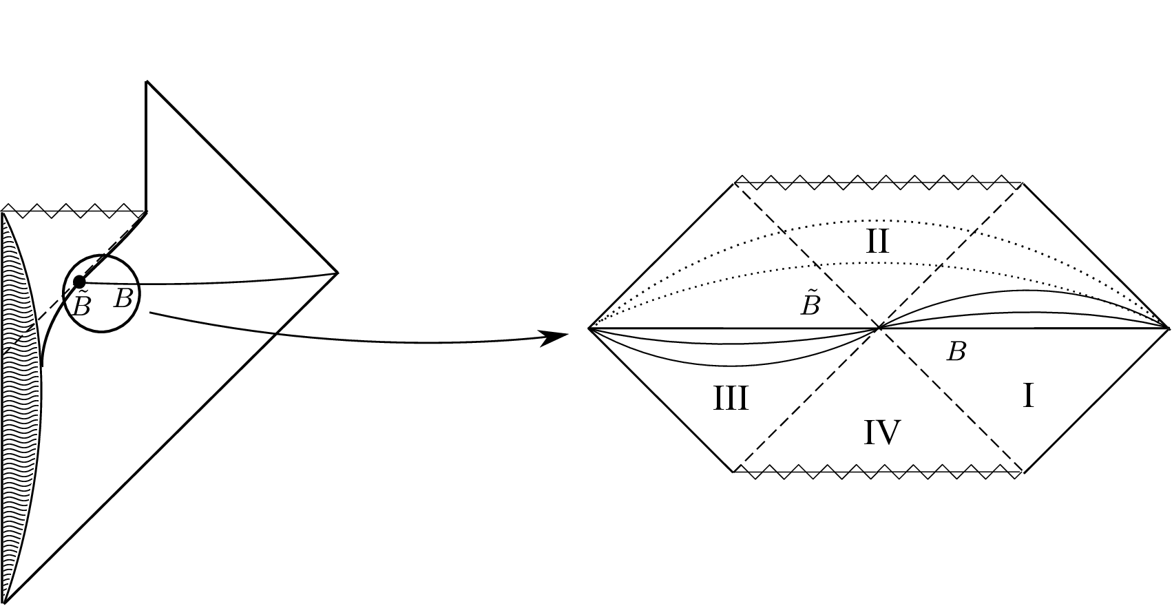
It is important that this identification mapping is made in each instant of time; for example, the mass of the corresponding eternal black hole must be taken as that of the evolving black hole at each moment. Note also that the identification with the eternal black hole is made only for the stretched horizon degrees of freedom and the outside states entangled with them; the structure of the other modes need not follow that of the eternal black hole. We can summarize these concepts by saying that an eternal black hole (of a fixed mass) provides a model for an evolving black hole for a timescale much shorter than that of the evolution. A schematic picture for this mapping is depicted in Fig. 1.
Key elements to understand physics of black holes (and firewalls) arising from the picture described above are
- •
The dimensions of the Hilbert spaces for the stretched horizon states and the states entangled with them are both , where is the area of the horizon and is the Planck length. The number of microscopic degrees of freedom needed to describe a black hole is thus . The actual black hole states, however, occupy only a tiny -dimensional subspace of the -dimensional Hilbert space relevant for these degrees of freedom [13], as suggested by black hole thermodynamics. All the other states represent “firewall states,” which do not allow for a semi-classical interpretation of the interior region.
- •
As long as the quantum state for the stretched horizon and the entangled modes stays in the -dimensional subspace, an infalling observer interacting with this state finds a smooth horizon with a probability of . This is because the -dimensional subspace is spanned by microstates all representing the same semi-classical black hole with a smooth horizon, and the internal dynamics of the horizon is such that an infalling object sees/measures the horizon in this basis [10]. The evolution of a black hole is consistent with the assumption that the relevant degrees of freedom keep staying in this subspace so that no firewall develops.
- •
Operators responsible for describing the exterior spacetime region act only on the modes outside the stretched horizon as implied by local quantum field theory applicable outside the stretched horizon. On the other hand, local operators responsible for describing the interior spacetime region act nontrivially both on the stretched horizon and the outside entangled modes. This “asymmetry” arises because the stretched horizon degrees of freedom represent the exterior modes outside the horizon in the other side of the eternal black hole under the identification map described above.
We find that these elements elegantly address the questions raised by the firewall argument. Representative results include
- •
The evolution of a black hole does not dynamically develop a firewall (even after the Page time [16]). An infalling observer who does not perform a special manipulation to his/her environment always sees a smooth horizon.
- •
It is not possible for an observer to see a firewall even if he/she performs a very special measurement on Hawking radiation emitted earlier from the black hole. Such a measurement cannot change the fact that he/she will see a smooth horizon.
- •
If a falling observer can directly measure a mode entangled with the stretched horizon as he/she falls through the horizon, then he/she may see a firewall. This, however, does not violate the equivalence principle; the same can occur at any surface in a low curvature region.
We note that the framework presented here and resulting physical predictions also apply to other horizons, including de Sitter and Rindler horizons, with straightforward adaptations. We will discuss these cases toward the end of the paper.
The organization of the rest of this paper is as follows. In Section 2, we describe the microscopic structure of the black hole vacuum states. In Section 3, we see how these states are embedded in the larger Hilbert space relevant for the stretched horizon degrees of freedom and the states entangled with them. We discuss how the vacuum and non-vacuum black hole states as well as the firewall states arise in this large Hilbert space, and identify the form of local operators responsible for describing the exterior and interior spacetime regions. We argue that the dynamics of quantum gravity can be such that a black hole stays as a black hole state under time evolution (not becoming a firewall state), and that an infalling observer interacting with such a state will see a smooth horizon with a probability of because of the properties of the internal dynamics of the horizon. In Section 4, we discuss the fate of infalling observers under various circumstances, especially when the observers manipulate degrees of freedom before entering the horizon. We also describe how the present framework is realized in an infalling reference frame. We argue that locally (and global) Minkowski vacuum states are not unique at the microscopic level, although the same semi-classical physics can be built on any one of them, so that this degeneracy need not be taken into account explicitly in usual applications of quantum field theory, e.g. to the problem of scattering. In Section 5, we discuss how our framework is applied to de Sitter horizons.
2 Microscopic Structure of Black Holes
Here we discuss the microscopic structure of black holes, following Refs. [10, 11, 12, 13, 14]. Suppose we describe a system with a black hole, which for simplicity we take to be a Schwarzschild black hole in 4-dimensional spacetime, from a distant reference frame. We assume that, for any fixed black hole mass , the entire system is decomposed into three subsystems:11 1 We adopt a notation close to that of Ref. [7], although the precise physical object each symbol represents sometimes differs.
- :
the degrees of freedom associated with the stretched horizon;
- :
the degrees of freedom associated with the spacetime region close to, but outside, the stretched horizon, e.g. ;
- :
the rest of the system (which may contain Hawking radiation emitted earlier).
Among all the possible quantum states for the degrees of freedom, some are strongly entangled with the states representing .22 2 We ignore possible tiny direct entanglement between and , which is a good approximation if the spacetime region for is taken sufficiently large. Note that the entanglement necessary for unitarity of the evolution of the state is not of this type; see later. We call the set of these quantum states :
- :
the quantum states representing the states for the degrees of freedom that are strongly entangled with the degrees of freedom described by .
Following the locality hypothesis, we consider that systems and , more precisely operators acting only on or , are responsible for physics outside the stretched horizon, which is well described by local quantum field theory at length scales larger than the fundamental (string) length . On the other hand, the interior spacetime for an infalling observer, as we will argue, is represented by operators acting on the combined system (on both and states). In our analysis below, we ignore the center-of-mass drift and spontaneous spin-up of black holes [17], which give only minor effects on the dynamics.
Suppose, as usual, we quantize the system in such a way that the Hamiltonian near (and outside) the horizon takes locally the Rindler form. Then, a black hole vacuum state is described by one in which some of the states for the degrees of freedom, i.e. , are (nearly) maximally entangled with the states for [18]. The basic idea of Refs. [10, 11] is that there are exponentially many ( where is the horizon area33 3 Here and below, similar expressions are valid at the leading order in expansion in powers of , in the exponent for the number of states (or in entropies). With this understanding, we will use the equal sign below, instead of the approximate sign.) black hole vacuum states which correspond to the same semi-classical black hole, and that there can be a (semi-)classical world built on each of them, all of which look identical to general relativity but are represented differently at the microscopic level (consistently with the no-hair theorem). More specifically, the states , which live in the combined system, can be written as [11, 13]
| (1) |
Here, are coefficients that satisfy the orthonormality condition and the condition for each being maximally entangled
| (2) |
and and () are elements of and with [13]
| (3) |
where and are the Hilbert space factors that contain all the possible states for and , respectively.
To be more precise, the black hole vacuum states are written as
| (4) |
instead of Eq. (1). Here, , and and are the energy of the state and the reciprocal of the temperature relevant for it (i.e. the effective blue-shifted local Hawking temperature relevant for the state). The expressions in Eqs. (1 – 3) are the ones in which the Boltzmann factors, , are ignored and is replaced by the effective Hilbert space dimension for the states, which we identify as the Hilbert space dimension for the states. The conditions in Eq. (2), therefore, must be regarded as approximate ones.
For simplicity, below we will use the expressions in Eqs. (1, 2) for ’s, which is a good approximation for our purposes. The more precise expression of Eq. (4), however, suggests why the number of independent black hole vacuum states is only , despite the fact that the dimension of the Hilbert space for the combined system is much larger, . If maximal entanglement between and were the only condition for a smooth horizon, then we would have smooth horizon black hole states. In order for the horizon to be smooth, however, the and states must be entangled in a particular Boltzmann weighted way; in particular, having energy must be multiplied by having exactly the opposite energy , not by some with . Here, the concept of energy for the states arises through identification of these states as the modes outside the horizon in the other side of an eternal black hole; see Section 3.3. Assuming that there are no states exactly degenerate in energy, this only leaves a room to put phase factors in front of various terms, leading to only (not ) independent states as shown in Eq. (4), where is the effective Hilbert space dimension for the states. Taking the number of independent black hole states to be as implied by the standard thermodynamic argument, the dimensions of and are fixed as in Eq. (3). As emphasized in Refs. [13, 14], this implies that space spanned by the states comprises only a tiny, -dimensional, subspace of the Hilbert space representing the combined system: .44 4 Incidentally, the Bekenstein-Hawking entropy may also be identified as the von Neumann entropy of a reduced density matrix for the combined system obtained after integrating out the horizon degrees of freedom , along the lines of Ref. [19]. For this identification to work, the fundamental length scale must scale as , where is the number of species appearing in low energy 4-dimensional field theory applicable at length scales larger than . We assume this is indeed the case (see e.g. [20]).
In general, a black hole vacuum state can be represented by an arbitrary density matrix defined in space spanned by the ’s. In the case where entanglement between the black hole and the rest may be ignored, the entire system can be written as
| (5) |
where is an element of , the Hilbert space factor comprising all the possible states for subsystem . If the black hole is formed by a collapse of matter that has not been entangled with its environment, then the state of the system is well approximated by Eq. (5) until later times (see below). With such a formation, the number of possible black hole microstates is expected to be much smaller than (presumably of order where is an coefficient [21]); but after the scrambling time [15], all these states are expected to evolve into generic states of the form in Eq. (5):
| (6) |
As time passes, the black hole becomes more and more entangled with the rest in the sense that the ratio of the entanglement entropy between and , , to the Bekenstein-Hawking entropy at that time, , keeps growing, which saturates the maximum value after the Page time , where is the initial mass of the black hole [16]. Therefore, the state of the system at late times must be written more explicitly as [10, 11, 12]
| (7) |
where ’s are elements of . In other words, at these late times the logarithm of the dimension of space spanned by ’s is of order (and equal to after the Page time), while at much earlier times it is negligible compared with . The state at early times, therefore, can be well approximated by Eq. (5) for the purpose of discussing internal properties of the black hole.
As we will see, the structure of the black hole states described above, together with dynamical assumptions discussed in Section 3, elegantly addresses questions raised by the firewall argument. Before turning to these issues, however, we make a comment on the structure of Hilbert space to avoid possible confusion. As described at the beginning of this section, we have divided the system with a black hole of mass into three subsystems , , and ; this division, therefore, implicitly depends on the mass . Since the black hole mass varies with time, the Hilbert space in which the state of the entire system evolves actually takes the form
| (8) |
where we have explicitly shown the dependence of , , , and , and as seen in Eq. (3). is the Hilbert space spanned by the states for the degrees of freedom orthogonal to (i.e. not entangled with ), and we define to be the Hilbert space for the system without a black hole. As the black hole evolves, the state of the system moves between different ’s; for example, a state that is an element of with some will later be an element of with .55 5 More precisely, the state at a later time will be a superposition of elements in various ’s, reflecting the probabilistic nature of Hawking emission. We ignore this effect, as well as a possible spread of the initial black hole mass caused, e.g., by quantum effects associated with the collapse, since they do not affect our argument.
To help understand the meaning of Eq. (8), let us consider a system in which a black hole was formed at time with the initial mass : . Suppose at some time with , the black hole mass is (). Then, the state of the system at that time, , is given (approximately) by an element of in the form of Eq. (5). Now, at a later time with , the mass of the black hole becomes smaller, (). The state of the system is then given by an element of that takes the form of Eq. (7) with (almost all) ’s linearly independent. Finally, after the black hole evaporates, the system is described by an element of (which is generally time-dependent, representing the propagation of Hawking quanta).
3 Black Hole Interior vs Firewalls
In this section, we discuss the structure of elements in the Hilbert space factor and operators acting on it, assuming that there is no extra matter near and outside the stretched horizon. (If there is extra matter, it simply changes the identification of the states in the Hilbert space for the degrees of freedom.) For simplicity, we focus our discussion mostly on these entities for a fixed . The evolution of a black hole, which leads to a variation of , is discussed in Section 3.4 only to the extent needed.
3.1 Black hole states and firewall states
Let the Hilbert space spanned by the black hole vacuum states be :
| (9) |
At the leading order, the dimension of is , i.e.
| (10) |
where . (Here and below we use the approximate symbol, , to indicate that an expression is valid at the leading order in expansion in inverse powers of .) The basic idea of Refs. [10, 11] is that a semi-classical world can be constructed on each of ’s, and that all of these worlds look identical to general relativity. In the language here, this implies that an operator that can be used to describe a semi-classical world for an infalling observer may be written in the block-diagonal form in the space
| (11) |
if an appropriate basis is chosen. Moreover, by taking an appropriate basis in each block, all the operators in the diagonal blocks , which we call branch world operators (and are represented here by matrices), may be brought into an identical form
| (12) |
The resulting basis states can be arranged in the form
| (13) |
where we have listed the basis states in in the form of a column vector; i.e., each block contains one of the black hole vacuum states ’s, and in each block the can be put at the bottom of the column vector of dimensions.
In the basis of Eq. (13), the outgoing creation/annihilation operators for an infalling observer ( or in Ref. [18] or in Ref. [6]) take the form of Eq. (11) with all the branch world operators taking the same form, which we denote by .66 6 Strictly speaking, a creation/annihilation operator acting on an element in may transform it into an element of with (slightly) different from . Here we do not treat this effect very explicitly, which can be done by considering an appropriate set of ’s (with appropriately coarse-grained ’s, if one wants) or by defining the creation/annihilation operators in such a way that when they act on an element in the resulting states stay in the same , by adjusting the mass associated with the singularity at the center. In any event, this issue is not crucial for the firewall argument, since it can be constructed using only number operators, e.g. , which transform an element of into that in the same . (For simplicity, below we only consider spherically symmetric modes to keep the shape of the horizon, but the extension to other cases is straightforward.) By acting (a finite number of) ’s on one of the ’s, one can construct a state in which matter exists in the interior of the black hole as viewed from an infalling observer. How many such states can we construct from a vacuum state , keeping the classical spacetime picture in the interior? We expect that the number of these states (for each ) is of order with [21]. This implies that the number of all the states in that allow semi-classical interpretation in the black hole interior is
| (14) |
Namely, the Hilbert space factor () spanned by all these semi-classical—i.e. not necessarily vacuum—black hole states satisfies
| (15) |
consistent with the counting expected by the holographic bound [21, 22]. As we will see more explicitly in the next subsection, an arbitrary superposition of elements of (or an arbitrary density matrix in ) represents a black hole state in which an infalling observer sees smooth horizon. In particular, this implies that in order for the infalling observer not to find any drama, the black hole state need not take the maximally entangled form in Eq. (1)—it can even be in a separable form of (without summation in ), since these states can be obtained as a superposition of (maximally entangled) ’s.
Once again, the condition for an infalling observer to see smooth horizon is not that a black hole (vacuum) state has a maximally entangled form, but that it stays in the -dimensional subspace (or ) in the -dimensional space (called the balanced form in Ref. [13] for the vacuum states). This is because as long as the black hole state stays in , the dynamics of the horizon makes the observer see the state in the basis determined by , as will be discussed more explicitly in the next subsection. This therefore replaces/refines (in a sense) the maximally-entangled condition of Ref. [23] for the existence of smooth classical spacetime (in the present context, beyond the horizon). The vast majority of the states in that do not belong to are “firewall states.” They do not admit the smooth classical spacetime picture in the interior of the horizon; in particular, they include states in which a diverging number of quanta, including high energy modes, are excited on . It may be possible to view these states as representing the situation in which singularities of general relativity exist near the horizon, not just at the center (see Ref. [24]), so that there is no classical spacetime in the interior region.
3.2 No firewall for black hole states—dynamical selection of the basis
We now argue that if the state stays in subspace in the Hilbert space factor , then an infalling observer does not see firewalls. We begin by discussing why operators responsible for describing (semi-)classical worlds for an infalling observer take the special block-diagonal form of Eqs. (11, 12). Why can’t general Hermitian operators acting on the -dimensional space be observables in these worlds?
As discussed in Refs. [5, 25], observables in classical worlds—which emerge dynamically from the full quantum dynamics—correspond, in general, to only a tiny subset of all the possible quantum operators acting on the microscopic state of the system. These observables represent the information that can be amplified in a single term in a quantum state (i.e. the information that can be shared and compared by multiple physical “observers” in the system), and are selected as a result of the dynamics of the system (the selection of the measurement basis). The statement that operators used to describe a semi-classical world for an infalling observer take the form of Eqs. (11, 12), therefore, comprises an assumption on the internal dynamics of the system, i.e. the microscopic Hamiltonian acting on the and degrees of freedom, which determines the form of operators representing observables in a semi-classical world [10]. In fact, this is precisely the physical content of the complementarity hypothesis, which has to do with how classical spacetime emerges in a full quantum theory of gravity. In the distant description, an object falling into the horizon will interact strongly with surrounding highly blue-shifted Hawking quanta, making it (re-)entangled with the basis determined by the ’s. Here we take this dynamical assumption for granted, which one might hope to eventually derive from the microscopic theory of the and degrees of freedom.
With this interpretation of semi-classical observables, it is now easy to see that an arbitrary state in , or more generally an arbitrary density matrix in , does not lead to a firewall for an infalling observer. Consider, for simplicity, that the and degrees of freedom are in a pure state
| (16) |
where ’s are arbitrary coefficients with . If the infalling observer interacts with this state, then he/she will “measure,” or “feel,” it in the basis determined by ’s in Eqs. (11, 12); i.e. he/she will find that the black hole is in a particular state with probability . Since all the states represent the same semi-classical black hole with smooth horizon (at the level of general relativity), this implies that the observer will find that the horizon is smooth with a probability of ---the observer does not see a firewall.77 7 This statement is exact if the measurement basis is selected perfectly by Eqs. (11, 12), which will indeed be the case in the limit that the system has an infinite number of degrees of freedom. Since the number of degrees of freedom is very large, though not infinite, this is an extremely good approximation—the correction, if any, will be exponentially suppressed by a factor of .
In fact, one can obtain the same conclusion by calculating the average number of high energy quanta (i.e. quanta with ) for the states in . In the basis of Eq. (13), the number operators for modes take the form
| (17) |
for all , since ’s are black hole vacuum states. The average number of high energy quanta is then
| (18) |
for any , where the traces are taken over arbitrary basis states in . (Note that is independent of the basis chosen.) Since an expectation value of a number operator, , is positive semi-definite, this implies that typical states in do not have firewalls. By the definition of , the same argument also applies to the states in .
In Ref. [8], a similar calculation was performed with the conclusion that typical black hole states do have firewalls. A crucial element in the calculation of Ref. [8] was the statement/assumption that the eigenstates of the number operator provide a complete basis for unentangled black hole states (see also [26]), where is the annihilation operator for a Killing mode that is located outside the stretched horizon. If this were true, then we could calculate the average number of high energy quanta for the black hole states , defined analogously to Eq. (18), by going to the basis spanned by the eigenstates. Now, the semi-classical relation
| (19) |
where and are some functions, implies that the expectation value of an -number operator in a eigenstate is for any . This would, therefore, give , implying that typical black hole states must have firewalls.
Why has our calculation led to the opposite conclusion? The key point is that with the structure of the Hilbert space discussed here, the traces over in Eq. (18) cannot be taken as those over eigenstates. Below, we examine this point more closely. While doing so, we also discuss the structure of quantum operators that can be used to describe the exterior and interior spacetime regions of the black hole.
3.3 Exterior and interior operators
As we have seen in Section 3.1, the creation/annihilation operators for quanta on ’s take the form of Eqs. (11, 12) (e.g. with and for outgoing modes), which generically act nontrivially both on the and degrees of freedom. In general, one may take a linear combination of these operators to construct operators that represent a mode localized in the exterior or interior of the horizon (with the latter viewed from an infalling observer). What form would such operators take?
Let us consider the annihilation operator for an outgoing mode that is localized outside the stretched horizon. We consider a mode in , i.e. a mode (significantly) entangled with stretched horizon degrees of freedom .88 8 In view of Eq. (4), such a mode has an energy of the order of, or smaller than, the local Hawking temperature. Modes that have significantly higher energies than local Hawking temperatures are not directly entangled with . This is the mode used in the argument of Ref. [8]. The operator can be constructed by taking a linear combination of creation/annihilation operators ’s with and . Because of the assumption that low energy physics outside the stretched horizon is well described by local quantum field theory built on () and degrees of freedom, this operator must take the form
| (20) |
i.e. act only on the degrees of freedom, where and are operators defined in -dimensional and -dimensional Hilbert spaces, respectively. The complementarity hypothesis asserts that semi-classical physics—in particular physics responsible for the Hawking radiation process—persists, implying that the relation in Eq. (19) must be preserved (with and interpreted as the corresponding operators in the full -dimensional Hilbert space). This implies that the action of the particular linear combination of ’s and ’s appearing in the right-hand side of Eq. (19) on must be trivial, so that takes the form of Eq. (20).
What about operators representing an interior mode? One might naively think that those operators, collectively written as , take the form , analogous to Eq. (20). However, the structure of the black hole vacuum states in Eq. (1) (or Eq. (4)) and that of the Hilbert space in Eq. (3) suggest that this is not the case. These structures are exactly those of near-horizon modes of an eternal black hole with the same mass . We therefore postulate that
-
The quantum mechanical structure of a black hole after the scrambling time (when formed by a collapse) is the same as that of an eternal black hole (even) at the microscopic level.
In particular, the relevant Hilbert space describing a black hole of mass has dimension (), not , although the dynamics will make the state sweep only -dimensional subspace of it as the time passes or as the initial condition for the collapse is scanned. (This sweeping will be ergodic in the subspace after a sufficient coarse-graining.) This is, obviously, consistent with the semi-classical expectation that a black hole formed by a collapse looks like an eternal black hole when it is probed late enough. Here we require that it is also the case quantum mechanically at the microscopic level, including the form of operators representing various excitations.
More precisely, we consider that the and degrees of freedom for a black hole of mass correspond, respectively, to the near-horizon degrees of freedom in one and the other external regions—often called regions I and III—of an eternal black hole with the same mass as viewed from a distant reference frame. (See Fig. 1 for a schematic depiction.) Here, the near-horizon modes are defined such that the reactions of the modes in region I to the exterior operators of the form in Eq. (20) are the same as those of ; for example, these modes have energies of the order of, or smaller than, local Hawking temperatures. The near-horizon modes in region III can then be defined through entanglement with those in region I. We assume that the Hilbert space structure of the and states for a collapse-formed black hole (often called a one-sided black hole) is the same as that of the states in the two exterior regions of an eternal black hole (two-sided black hole) with the quantization hypersurface taken as an equal-time hypersurface determined by the outside timelike Killing vector. This suggests that operators responsible for describing the interior spacetime region take the form
| (21) |
where is defined in the full -dimensional Hilbert space , while and are defined in -dimensional Hilbert spaces and , respectively.
The structure of operators in Eq. (21) can be motivated by the fact that an equal-time hypersurface determined by the outside timelike Killing vector forms a Cauchy surface, so that all the local operators in the interior spacetime can be obtained by evolving local operators of the form on the initial equal-time hypersurface along a set of hypersurfaces depicted by dotted lines in the right panel of Fig. 1. (Note that this evolution preserves this particular form of operators, since it can be represented by acting some unitary operator and its inverse from left and right, respectively.) We assume that the interior region of the black hole under consideration can be constructed in this way with and acting only on the near-horizon modes in the respective regions, leading to Eq. (21). We emphasize again that the “identification” of the and states with the eternal black hole states is made at each instant of time (or in a sufficiently short time period compared with the timescale for the evolution of the black hole); in particular, the mass of the eternal black hole must be taken as that of the evolving black hole at each moment , not the initial mass . This implies that an infalling object passes through the horizon of the eternal black hole at the center of the Penrose diagram depicted in the right panel of Fig. 1.
We are now at the position of discussing why our analysis in Section 3.2 has led to the opposite conclusion as that in Ref. [8]. The key point is that in our present framework, the black hole vacuum states provide a complete basis of the (-dimensional) Hilbert space (), while the eigenstates provide that of a different (again, -dimensional) Hilbert space . This implies, in particular, that the black hole vacuum states can not all be made eigenstates by performing a unitary rotation in the space spanned by (i.e. ) in which the traces in Eq. (18) are taken. This can be seen more explicitly as follows. Let us write ’s in the form of Eq. (1). Since the eigenstates span a basis in , we may write as
| (22) |
where ’s are the eigenstates. (Note that these eigenstates may be degenerate; i.e., and with need not have different eigenvalues under .) Substituting Eq. (22) into Eq. (1), we obtain
| (23) |
where
| (24) |
An important point is that the element in that is entangled with , i.e. , depends on the vacuum state, i.e. on the index . This prevents us from finding a basis change in that makes all the ’s eigenstates. (Otherwise, the rotation represented by the matrix would do the job.) The traces in Eq. (18), therefore, cannot be taken over eigenstates, avoiding the conclusion in Ref. [8].
3.4 Dynamical evolution
We have seen that the and degrees of freedom can represent very different objects—black holes and firewalls—depending on their quantum mechanical states. In particular, if they are in a state that is an element of -dimensional Hilbert space (or represented by a density matrix that is an element of ), then an infalling observer interacting with these degrees of freedom will find that the horizon is smooth and see the interior spacetime; if not, he/she will see a firewall. (In general, if the state involves a component in , the infalling observer will see the interior spacetime with the corresponding probability.) Here, we have restored the index to remind us that is, in fact, a component of ; see Eq. (8).
A natural interpretation of these black hole and firewall states—i.e. the elements of —is that they both represent objects that lead to the Schwarzschild spacetime of mass in the region outside the (stretched) horizon, because they both use the same () and degrees of freedom and local quantum field theory is supposed to be valid in this region. A crucial question then is: what does the dynamics of the (entire) system tell us about the properties of an object under consideration? In particular, if the object is formed by a collapse of matter with the initial mass , are the corresponding and degrees of freedom in a state in (or )? And if so, do they stay in (or ) when the mass is reduced to () by time evolution?
We do not know a priori the answer to these questions. We may, however, interpret the success of general relativity with the global spacetime picture to mean that the dynamical evolution keeps the degrees of freedom to stay in subspace (or ), i.e. in a state that allows for the smooth classical spacetime interpretation in the interior of the horizon (at least, in the absence of a certain special manipulation of the degrees of freedom by an infalling observer; see Section 4). This interpretation can be made particularly plausible by considering the extension of the framework to (meta-stable) de Sitter space, where the validity of the global spacetime picture beyond the de Sitter horizon is strongly supported by the successful prediction for density perturbations in the inflationary universe; see Section 5. We therefore postulate that the dynamics of quantum gravity is such that it keeps an element of (or ) to stay in (or ) under time evolution, where in general. In the context of black hole physics, this implies that the state of the system takes the form of Eq. (5) when the black hole is formed by (isolated) matter, which evolves into Eq. (7) as time passes. This evolution is indeed consistent with the standard dynamics for the black hole evaporation process, e.g. the generalized second law of thermodynamics. An explicit qubit model representing this process was described in Ref. [14].
As discussed in Ref. [10], the evolution described above is also consistent with the standard analysis of the information flow in black hole evaporation in a unitary theory of quantum gravity [16], avoiding the paradox raised by Ref. [6]. (In fact, this was how the structure of the black hole states discussed in this paper was first found.) In Ref. [6], it was argued that for an old black hole, the conditions for unitarity and smooth horizon, which were respectively given by
| (25) |
were mutually incompatible, where represents the von Neumann entropy of subsystem . The structure of the black hole states discussed here, however, elegantly avoids this conclusion, keeping the standard assumptions of black hole complementarity. For a state with an old black hole given in Eq. (7), the conditions for unitarity and smooth horizon are given, respectively, by [10]
| (26) |
where are branch world entropies, the von Neumann entropy of subsystem calculated using the state representing the (semi-)classical world : (without summation in the right-hand side). The point is that the relations in Eq. (26) are not incompatible with each other; in fact, they are all satisfied for a generic state of the form of Eq. (7) after the Page time. The reason for this success can be put as follows:
-
What is responsible for unitarity of the evolution of the black hole state is not an entanglement between early radiation and modes in as imagined in Ref. [6], but an entanglement between early radiation and the way and degrees of freedom are entangled.
In other words, the information of the black hole is contained in the coefficients in Eq. (7), i.e. how the black hole is made out of the vacuum states.
3.5 Gauge/gravity duality
Here we comment on how a black hole (or a firewall) may be realized in the gauge theory side of gauge/gravity duality. As an example, we might consider a setup in Ref. [7] in which an evaporating black hole is modeled by a conformal field theory (CFT) coupled to a large external system. How can the structure discussed in this paper be realized in such a setup?
One possibility is that the whole structure of the Hilbert space described so far, in particular the Hilbert space of dimensions for the horizon and the entangled degrees of freedom, exists at the microscopic level in the corresponding gauge theory. The whole degrees of freedom are not visible in standard thermodynamic considerations in the gauge theory side, since the dynamics populates only the subspace () of the whole Hilbert space () relevant for these degrees of freedom. The local operators responsible for describing the exterior and interior regions are still given in the form of Eqs. (20) and (21), respectively. We note that a similar construction of operators in the exterior and interior regions were discussed in Ref. [27], in which the degrees of freedom were thought to arise effectively after coarse-graining the outside degrees of freedom. Our picture here is different—we consider that both the stretched horizon () and the outside () degrees of freedom exist independently at the microscopic level. It is simply that standard black hole thermodynamics does not probe all the degrees of freedom because of the properties of the dynamics.
An alternative possibility is that the gauge theory only contains states in for the horizon and the entangled degrees of freedom.99 9 We thank Donald Marolf for discussions on this point. In this case, the gauge theory cannot describe a process in which the state for these degrees of freedom is made outside (i.e. creation of a firewall), or it may simply be that such a process does not exist in the gravity side as well (see a related discussion in Section 4.1).
4 Infalling Observer
In this section, we discuss what our framework predicts for the fate of infalling observers under various circumstances. We also discuss how the physics can be described in an infalling reference frame, rather than in a distant reference frame as we have been considering so far.
4.1 Physics of an infalling observer: a black hole or firewall?
As we have seen, as long as the black hole state is represented by a density matrix in , an infalling observer interacting with this state sees a smooth horizon with a probability of . Here we ask what happens if the observer manipulates the relevant degrees of freedom, e.g. measures some of the or modes, before entering the horizon. This amounts to asking what black hole state such an observer encounters when he/she falls into the horizon.
We first see that the observer finds a smooth horizon with probability no matter what measurement he/she performs on Hawking radiation emitted earlier from the black hole. This statement is obvious if the object the observer measures is not entangled with the black hole, e.g. as in Eq. (5), so we consider the case in which the observer measures an object that is entangled with the black hole. To be specific, we consider the case in which the observer measures the degrees of freedom in Eq. (7) before he/she enters the black hole. Without loss of generality, we assume that the outcome of the measurement was , where is an arbitrary unitary matrix. The state of the black hole the observer encounters is then . Since this is a superposition of the black hole states ’s, the observer finds a smooth horizon with a probability of , as discussed in Section 3.2. We conclude that it is not possible to create a firewall by making a measurement on early Hawking radiation.
On the other hand, if an infalling observer can directly access the states entangled with the stretched horizon modes, then he/she may be able to see a firewall. Consider that the black hole state is given by Eq. (7). We may then expand the states in terms of the eigenstates as in Eq. (22), leading to
| (27) |
where and are given in Eqs. (23, 24). Suppose the observer measures the degrees of freedom are in a eigenstate . Then the relevant state is
| (28) |
without summation in . Now, the state is in general a superposition of decohered classical states , ,1010 10 The reason for this decomposition is that decohered terms in a state must be treated as different worlds when calculating probabilities. Note that the way is decomposed into ’s is not important for our discussion (which simply alters the values of ), i.e. our conclusion is not affected by the way this decoherence happens. so the observer finds the state is in one of the ’s, where
| (29) |
This state is not in general a superposition of the smooth horizon states ’s; in other words, is not an element of . Thus, if the infalling observer directly measures to be in a eigenstate (which will require the detector to be finely tuned) and enters the horizon right after (i.e. before the state of the black hole changes), then he/she will see a firewall with an probability.1111 11 There is a small probability that the observer still sees a smooth horizon, since a superposition of different states in Eq. (28) in which the firewall terms are canceled must be able to reproduce the smooth horizon state, Eq. (27). Here we have assumed that such a measurement can be performed, although it is possible that there is some dynamical (or perhaps computational [28]) obstacle to it. We note that a similar argument to the one here applies to any surface in a low curvature region, not just the black hole horizon. This way of seeing a firewall, therefore, does not violate the equivalence principle.
We finally mention that even if an observer finds to be in a eigenstate, if he/she enters the horizon long after that, then he/she may see a smooth horizon rather than a firewall. Suppose that the observer measured a eigenstate when the black hole had mass . This implies that he/she was entangled with the eigenstate in , where we have explicitly shown the dependence of the decomposition. Now, at a much later time, the black hole has a smaller mass (). The mode which was in may then be in . If this is the case, then the observer is no longer entangled with a mode necessary to see a firewall, i.e. ; instead, he/she is simply entangled with the environment (early radiation) of the black hole, . This observer will therefore see a smooth horizon when he/she enters the black hole, as discussed at the beginning of this subsection. The fact that an observer was once entangled with a mode is not enough to see a firewall; he/she must be entangled with a mode of the black hole at the time of entering the horizon in order to see a firewall.
4.2 Description in an infalling reference frame
We now consider how the physics for an infalling object is described in an infalling reference frame, rather than in a distant frame as has been considered so far. Following Ref. [5], we consider that such an infalling description is obtained by performing a unitary transformation on the distant description, corresponding to a change of the clock degrees of freedom in full quantum gravity. According to the complementarity hypothesis, the Hamiltonian—the generator of time evolution—after the transformation takes the form local in infalling field operators, including the interior operators discussed in Section 3.3.
Since the complementarity transformation is supposed to be unitary, the states must be transformed into different states which must all look like locally Minkowski vacuum states. In particular, this implies that in the limit that the black hole is large , i.e. in the limit that the horizon under consideration is a Rindler horizon, there are infinitely many Minkowski vacuum states labeled by . This seems to contradict our experience that we can do physics without knowing which of the Minkowski vacua we live in. Isn’t the Minkowski vacuum unique, e.g., in QED? Otherwise, we do not seem to be able to do any physics without having the (infinite amount of) information on the Minkowski vacua.
The structure of operators discussed in Section 3.1, however, provides the answer. After the complementarity transformation, the form of operators is preserved; in particular, all the local operators responsible for describing semi-classical physics take the block-diagonal form, Eq. (11), with all the (branch world) operators in the diagonal blocks taking the identical form, Eq. (12). This implies that no matter which superposition of Minkowski vacua we live in, we always find the same semi-classical physics (which is everything in the non-gravitational limit). More precisely, if we live in a vacuum represented by state (), then we find ourselves to be in a particular vacuum with probability (i.e. the measurement basis is ), but all of these vacua lead to the same semi-classical physics. In order to discriminate different vacua, we need to consider operators beyond local field operators, e.g. those of Eq. (11) with taking different forms for different in the basis of Eq. (13). Such operators will be either highly nonlocal or act on the boundary/horizon of the infalling/locally Minkowski description of spacetime. In the true Minkowski space, the boundary is located only at spatial infinity. In the case of an infalling description of a black hole vacuum, however, spacetime is Minkowski vacuum-like only locally, and the nonzero curvature effect can lead to a horizon (as viewed from the infalling frame, not the original one as viewed from a distant frame) at a finite spatial distance, e.g. along the lines of Ref. [12]. Probing microscopic degrees of freedom on such a horizon, therefore, might allow us to access the information on which vacuum the observer is in.
5 de Sitter Space
The quantum theory of horizons described in this paper is applicable to horizons other than those of black holes with straightforward adaptations. Here we discuss an application to de Sitter horizons. The analysis is parallel with the case of black hole horizons.
The de Sitter horizon is located at in de Sitter space, where is the radial coordinate of the static coordinate system and the Hubble parameter. The stretched horizon is located where the local Hawking temperature
| (30) |
becomes of order the fundamental/string scale : (the factor of is for convenience), i.e.
| (31) |
Following the analysis of the black hole case, we consider that the dimensions of the Hilbert spaces for the stretched horizon degrees of freedom, , and the states entangled with them, , are given by
| (32) |
where is the area of the (stretched) de Sitter horizon. We may expect that at the leading order in , the dimension of the Hilbert space spanned by all the possible states inside the de Sitter horizon () is the same as that of , which we assume to be the case. (As can be seen from the distribution of thermal entropy , most of these states are localized near the horizon.) The dimension of the total Hilbert space needed to describe de Sitter space is then
| (33) |
at the leading order in .
As in the case of black holes, the states which allow for the interpretation of classical spacetime outside the de Sitter horizon span only a tiny subspace of the entire Hilbert space
| (34) |
In fact, the Hilbert space spanned by the vacuum states already has the same logarithmic dimension at the leading order in :
| (35) |
with the basis states for measurement taking the maximally entangled form as in Eq. (1) (ignoring Boltzmann factors). As long as a state stays in (or is represented by a density matrix in ), an object that hits the horizon can be thought of going to space outside the horizon; otherwise, it hits a firewall/singularity. The information about the object that goes outside will be stored in the degrees of freedom, which may later be recovered, for example if the system evolves into Minkowski space (or another de Sitter space with a smaller vacuum energy). As in the black hole case, we expect that the dynamics of quantum gravity is such that a state in keeps staying in . In fact, this is observationally indicated by the success of the prediction for density perturbations in the inflationary universe, which is based on the global spacetime picture of general relativity [29].
Finally, we consider the limit in which the de Sitter space approaches Minkowski space. In this limit, the number of vacuum states becomes infinity
| (36) |
each differing in the way and states are entangled; see Eq. (1). Since most of the states are localized near the horizon, which is located at spatial infinity in this limit, probing the structure of (infinitely many) Minkowski vacua will require access to the boundary at infinity. This is the same picture we have arrived at in Section 4.2 by taking the large mass limit of a black hole horizon.
The fact that various horizons, especially black hole and de Sitter horizons, can be treated on an equal footing is an important ingredient for the quantum mechanical treatment of the eternally inflating multiverse advocated in Refs. [30, 5], in which the eternally inflating multiverse and the many worlds interpretation of quantum mechanics are unified as the same concept. It would be interesting to see if there are other implications of the present framework beyond what have been discussed in this paper.
Acknowledgments
We thank Juan Maldacena for useful conversations. This work was supported in part by the Director, Office of Science, Office of High Energy and Nuclear Physics, of the US Department of Energy under Contract DE-AC02-05CH11231, and in part by the National Science Foundation under grant PHY-1214644.
References
- [1] For reviews, see e.g. J. Preskill, in Blackholes, Membranes, Wormholes and Superstrings, ed. S. Kalara and D. V. Nanopoulos (World Scientific, Singapore, 1993) p. 22 [hep-th/9209058]; L. Susskind and J. Lindesay, An Introduction to Black Holes, Information and the String Theory Revolution: The Holographic Universe (World Scientific, Singapore, 2005).
- [2] L. Susskind, L. Thorlacius and J. Uglum, Phys. Rev. D 48, 3743 (1993) [arXiv:hep-th/9306069].
- [3] C. R. Stephens, G. ’t Hooft and B. F. Whiting, Class. Quant. Grav. 11, 621 (1994) [arXiv:gr-qc/9310006].
- [4] J. D. Bekenstein, Phys. Rev. D 7, 2333 (1973); S. W. Hawking, Commun. Math. Phys. 43, 199 (1975) [Erratum-ibid. 46, 206 (1976)].
- [5] Y. Nomura, Found. Phys. 43, 978 (2013) [arXiv:1110.4630 [hep-th]].
- [6] A. Almheiri, D. Marolf, J. Polchinski and J. Sully, JHEP 02, 062 (2013) [arXiv:1207.3123 [hep-th]].
- [7] A. Almheiri, D. Marolf, J. Polchinski, D. Stanford and J. Sully, arXiv:1304.6483 [hep-th].
- [8] D. Marolf and J. Polchinski, arXiv:1307.4706 [hep-th].
- [9] For earlier work, see S. L. Braunstein, arXiv:0907.1190v1 [quant-ph]; S. D. Mathur, Class. Quant. Grav. 26, 224001 (2009) [arXiv:0909.1038 [hep-th]]; S. B. Giddings, Class. Quant. Grav. 28, 025002 (2011) [arXiv:0911.3395 [hep-th]].
- [10] Y. Nomura and J. Varela, JHEP 07, 124 (2013) [arXiv:1211.7033 [hep-th]].
- [11] Y. Nomura, talk at SITP firewall meeting, Stanford, November 2012; talk at TH-institute: Black hole horizons and quantum information, CERN, March 2013.
- [12] Y. Nomura, J. Varela and S. J. Weinberg, arXiv:1304.0448 [hep-th].
- [13] E. Verlinde and H. Verlinde, arXiv:1306.0515 [hep-th].
- [14] E. Verlinde and H. Verlinde, arXiv:1306.0516 [hep-th].
- [15] P. Hayden and J. Preskill, JHEP 09, 120 (2007) [arXiv:0708.4025 [hep-th]]; Y. Sekino and L. Susskind, JHEP 10, 065 (2008) [arXiv:0808.2096 [hep-th]].
- [16] D. N. Page, Phys. Rev. Lett. 71, 3743 (1993) [hep-th/9306083].
- [17] D. N. Page, Phys. Rev. Lett. 44, 301 (1980); Y. Nomura, J. Varela and S. J. Weinberg, Phys. Rev. D 87, 084050 (2013) [arXiv:1210.6348 [hep-th]].
- [18] W. G. Unruh, Phys. Rev. D 14, 870 (1976).
- [19] R. D. Sorkin, in 10th International Conference on General Relativity and Gravitation, Contributed Papers, vol. II, 1167, eds. B. Bertotti, F. de Felice, and A. Pascolini (Roma, Consiglio Nazionale Delle Ricerche, 1983); L. Susskind and J. Uglum, Phys. Rev. D 50, 2700 (1994) [hep-th/9401070]; J. H. Cooperman and M. A. Luty, arXiv:1302.1878 [hep-th].
- [20] G. Dvali, Fortsch. Phys. 58, 528 (2010) [arXiv:0706.2050 [hep-th]].
- [21] G. ’t Hooft, gr-qc/9310026.
- [22] L. Susskind, J. Math. Phys. 36, 6377 (1995) [arXiv:hep-th/9409089]; R. Bousso, JHEP 07, 004 (1999) [arXiv:hep-th/9905177].
- [23] M. Van Raamsdonk, Gen. Rel. Grav. 42, 2323 (2010) [Int. J. Mod. Phys. D 19, 2429 (2010)] [arXiv:1005.3035 [hep-th]].
- [24] L. Susskind, arXiv:1208.3445 [hep-th].
- [25] See also, H. Ollivier, D. Poulin and W. H. Zurek, Phys. Rev. Lett. 93, 220401 (2004) [arXiv:quant-ph/0307229]; R. Blume-Kohout and W. H. Zurek, Phys. Rev. A 73, 062310 (2006) [arXiv:quant-ph/0505031].
- [26] R. Bousso, talk at TH-institute: Black hole horizons and quantum information, CERN, March 2013; arXiv:1308.2665 [hep-th].
- [27] K. Papadodimas and S. Raju, arXiv:1211.6767 [hep-th].
- [28] D. Harlow and P. Hayden, JHEP 06, 085 (2013) [arXiv:1301.4504 [hep-th]].
- [29] S. W. Hawking, Phys. Lett. B 115, 295 (1982); A. A. Starobinsky, Phys. Lett. B 117, 175 (1982); A. H. Guth and S.-Y. Pi, Phys. Rev. Lett. 49, 1110 (1982); J. M. Bardeen, P. J. Steinhardt and M. S. Turner, Phys. Rev. D 28, 679 (1983).
- [30] Y. Nomura, JHEP 11, 063 (2011) [arXiv:1104.2324 [hep-th]]; Phys. Rev. D 86, 083505 (2012) [arXiv:1205.5550 [hep-th]].