Nuclear dependencies of azimuthal asymmetries in the Drell-Yan process
Abstract
We study nuclear dependencies of azimuthal asymmetries in the Drell-Yan lepton pair production in nucleon-nucleus collisions with polarized nucleons. We use the “maximal two-gluon correlation approximation,” so that we can relate the transverse-momentum-dependent quark distribution in a nucleus to that in a nucleon by a convolution with a Gaussian broadening. We use the Gaussian ansatz for the transverse momentum dependence of such quark distribution functions and obtain the numerical results for the nuclear dependencies. These results show that the -integrated azimuthal asymmetries are suppressed.
pacs
25.75.Nq 13.85.Qk 13.88.+e 12.38.MhI introduction
Both the deep inelastic scattering (DIS) off hadrons and the Drell-Yan (DY) process in hadron-hadron collision have been playing very important roles in studying the structure of hadrons and the dynamics of quantum chromodynamics (QCD). Correspondingly, the DIS off nuclei and the DY process in hadron-nucleus collisions are also very important in studying the nuclear structure and the properties of cold nuclear matter. By studying the corresponding semi-inclusive processes, we can study not only the longitudinal but also the transverse momentum dependence of the parton distribution functions. In this connection, the semi-inclusive DY process is even more suitable to study the structure of hadrons or that of nuclei because no fragmentation function is involved. Azimuthal asymmetries are often sensitive physical variables for such studies and thus have attracted much attention [1, 2, 3, 4, 5, 6, 7, 8, 9, 10, 11, 12, 13, 14].
When a parton transmits through nuclear matter, the multiple gluon scattering with the nuclear matter leads to energy loss and transverse momentum broadening [16, 17, 15, 18, 19, 20, 21, 22, 23, 24, 25, 26, 27]. The multiple parton interaction results in also nuclear dependencies of azimuthal asymmetries. This provides a good alternative probe of properties of the nuclear matter. The nuclear dependence of the azimuthal asymmetry in semi-inclusive deep inelastic scattering (SIDIS) has been studied recently [28, 29, 30]. In this paper, we extend the study in Refs.[28, 29] to the DY process in nucleon-nucleus collisions. In Sec. II, we review the result of the differential cross section in the DY process with the polarized nucleon beam in terms of the transverse-momentum-dependent(TMD) parton distributions up to twist-2 level. In Sec. III, we study the nuclear dependence of the angular distribution of the DY lepton pair by relating the TMD quark distributions in a nucleus to that in a nucleon. We also illustrate the numerical results with an ansatz of the TMD parton distributions in a Gaussian form. We give a brief summary in Sec. IV.
II Differential cross section and azimuthal asymmetries
We consider the semi-inclusive DY process in nucleon-nucleus collisions with the transversely or longitudinally polarized nucleon beam,
| (1) |
where , , , , and are the four-momenta of the beam nucleon, one nucleon in the nucleus target, the virtual photon, the anti-lepton, and the lepton, respectively, and denotes the polarization vector of the incident nucleon. We use the light cone coordinate by introducing two light like vectors, and , and express the momenta and as
| (2) | |||||
| (3) |
where , , and denotes the mass of the nucleon. We restrict our study to the kinematic region where the transverse momentum of the DY pair is much less than its invariant mass . In this case, the differential cross section for the semi-inclusive DY process can be calculated in the framework of the TMD factorization theorem [31, 32]. Such calculations have been carried out for hadron-hadron collisions; the results can be found in, e.g., Refs.[33, 34, 35]. We note that such calculations can be extended to nucleon-nucleus collisions in a straightforward way and, at the twist-2 level, the differential cross section is given by
| (4) |
where and are, respectively, the helicity and the transverse polarization vector of the nucleon; , , and are, respectively, polar and azimuthal angles of the lepton pair and azimuthal angle of the polarization vector of the nucleon with respect to the transverse vector in the Collins-Soper frame. The ’s ( through ) are functionals of and that are defined as convolutions weighted by ,
| (5) | |||||
where and are the TMD distribution and/or correlation functions of quarks or anti-quarks. The superscript or denotes whether it is for the nucleon or the nucleus, and and in the arguments denote the flavor of the quark and whether it is for the quark or the anti-quark. The weights are given by
where . All the parton distribution and correlation functions, ’s and ’s, given in Eq.(4) are defined by the twist-2 decomposition of the quark correlation matrix [36, 37, 38],
| (6) | |||||
where with the total antisymmetric tensor and the definition of the components of are given by,
| (7) |
where is the gauge link that is necessary to ensure the gauge invariance of the matrix. In the DY process, the gauge link in covariant gauge is given by
| (8) |
where
| (9) |
It should be noted that the distribution function in Eq. (4) is defined as the mixture of and ,
| (10) |
We see that the differential cross section is determined by six TMD quark and anti-quark distributions and correlation functions , , , , , and . Each of them represents a given aspect of the parton structure of the nucleon, e.g., is the Sivers function[39, 40] which describes the correlation between the transverse momentum distribution and the transverse polarization of the nucleon, and is the Boer-Mulders function [41], which describes the correlation between the transverse quark momentum distribution and the transverse quark polarization in an unpolarized nucleon. In the TMD factorization formalism, all these distribution functions are unknown and cannot be calculated perturbatively. They can usually be obtained from parameterizations of experimental data or from model calculations (see, e.g., Refs. [42, 43, 44, 45, 46, 47, 48, 49, 50, 51, 52, 53, 54, 55, 56, 57, 58, 59, 60, 61, 62, 63, 64]). We should also note that these correlation functions such as the Sivers and the Boer-Mulders functions reflect not only the intrinsic motion of a parton inside a nucleon but also the multiple gluon scatterings (referred as initial or final state interaction) contained in the gauge link. In this connection, we recall the proof of Collins [65] that Sivers function is zero if we take the gauge link as unity. The same conclusion applies to the Boer-Mulders function. An intuitive but semiclassical picture for the non-zero Sivers function or the existence of left-right single-spin asymmetry was proposed in the 1990s[66] where one invokes the orbital angular momentum of quark and differentiates between the “front” and “back” surface of a nucleon due to the initial state interaction. This agrees qualitatively with the field theoretical calculations later on by Brodsky, Hwang, and Schmidt [67], where they use a non-zero orbital angular momentum of quark and take the initial state interaction into account explicitly and obtain a nonzero result for the Sivers function. Apparently, the same picture lead also to nonzero Boer-Mulders function.
We can integrate over the polar angle in Eq.(4) and obtain
| (11) |
We see that there are five kinds of different azimuthal asymmetries that are given by the average of , , , , and respectively. In terms of parton distribution and correlation functions, they are given by
| (12) | |||||
| (13) | |||||
| (14) | |||||
| (15) | |||||
| (16) |
where the subscript denotes the nucleon-nucleus collisions. They differ from those for nucleon-nucleon collisions only by the quark distribution and/or correlation functions as given by Eq. (7).
We also note that these asymmetries exist in collisions with the unpolarized, longitudinally polarized, and transversely polarized nucleon beams. In the unpolarized case, only exists and is determined by the Boer-Mulders functions . There is one single spin-asymmetry (SSA) in collisions with the longitudinally polarized beam, and it is determined by the longitudinal transversity and the Boer-Mulders function . There are three SSAs in collisions with the transversely polarized beam. They are represented by , , and . The well-known SSA is determined by the Sivers function , while and are determined by the Boer-Mulders function together with the pretzelosity or mixed from and respectively. Although we still do not know much about them, these functions have been studied in semi-inclusive DIS [68, 69, 70, 71] and some rough parameterizations have already been made [72, 73, 55, 43, 44].
III Nuclear dependence
It has been shown [24, 28] that multiple gluon scattering represented by the gauge link given by Eq. (8) leads to a strong nuclear dependence of the TMD parton distribution and/or correlation functions. Because all the asymmetries presented above are functionals of these parton correlation functions, we expect strong nuclear dependence of these asymmetries. We discuss them in the following.
III.1 Nuclear dependence of the TMD parton correlation function
In Ref. [24], with the assumption that the nucleus is large and weakly bound, the multiple-nucleon correlation can be neglected; the nuclear effect can only arise from the final state interaction in the form of multiple gluon scattering that is encoded into the gauge link in the definition of the TMD parton distributions. The important trick for the derivations is that the TMD quark distributions in nucleons or nuclei can be rewritten as a sum of higher-twist collinear parton matrix elements,
| (17) |
where is the parton transport operator and is given by
| (18) |
with being the covariant derivative. For simplicity, we have chosen the light-cone gauge in which the collinear gauge link disappears in the above. The nuclear effect arises when the the parton transport operator acts on the different nucleons. Under the “maximum two-gluon correlation approximation” [24], the nuclear TMD parton distribution has been expressed in terms of a Gaussian convolution of the same TMD distribution in a nucleon, i.e.,
| (19) |
where denotes the total average squared transverse momentum broadening. Furthermore, it has been shown in Ref.[28] that the relation can be extended to a much more general case so that
| (20) | |||||
where the components of the matrix are defined in Eq.(7). A somewhat different derivation can be found in Ref. [23, 74] where they resumed all the possible gluon exchange attached to different nucleons in the nucleus and obtained a diffusion equation that leads to the Gaussian convolution, the same result as that obtained in Ref. [24]. Recently it has been shown [75] that such simple Gaussian convolution will be broken by the process-dependent gauge links in cold nuclear matter when the finite volume effects are considered. In Ref. [24] and the current paper, we consider the limiting case of very large nuclei and neglect the finite volume effects. In the approach presented in Ref. [75], the authors try to study the finite volume effects where they have to take some specified model and consider the process-dependent gauge links. Their results are much more complicated than those obtained in Refs. [24] and [23, 74] and they find that the simple Gaussian convolution is broken. Here, in this paper, we consider the simple case as considered in Refs. [24] and [23, 74] and take the simple Gaussian convolution in the following.
For the DY azimuthal asymmetries presented in last section for nucleon-nucleus collisions, besides the TMD quark distribution , the Boer-Mulders distribution in the nucleus is also involved. From the decomposition in Eq. (7), we can express the Boer-Mulders distribution as the following
| (21) |
From the relation (20), we can show that the Boer-Mulders function in the nucleus is related to that in the nucleon in the exactly same way as the twist-3 distribution in Ref. [28], i.e.,
| (22) |
If we take the Gaussian ansatz for the transverse momentum dependence, i.e.,
| (23) | |||||
| (24) |
where we have assumed different flavors have the same Gaussian widths for the same types of TMD distributions and we have suppressed the flavor index. We obtain from Eqs. (19) and (22) that
| (25) | |||||
| (26) |
III.2 Nuclear dependence of the azimuthal asymmetry
It follows that azimuthal asymmetry in nucleon-nucleon and nucleon-nucleus collisions are given by, respectively,
| (27) | |||||
| (28) |
where we have defined a shorthand notation,
| (29) |
It is obvious that we can obtain by simply setting in . Hence we only present in the other azimuthal asymmetries in the following discussion.
The nuclear effect of the azimuthal asymmetry can be measured by the ratio,
| (30) |
In the special case where , we can obtain a simplified result
| (31) |
which means that the azimuthal asymmetry in the DY process in nucleon-nucleus collisions is suppressed compared to that in nucleon-nucleon collisions and has no dependence on the transverse momentum of the lepton pairs. It is very interesting that the suppression in Eq. (31) is very similar way to that of azimuthal asymmetry in SIDIS obtained in Ref. [29]. For the general case, the nuclear modification factor can only depend on three independent variables:
| (32) |
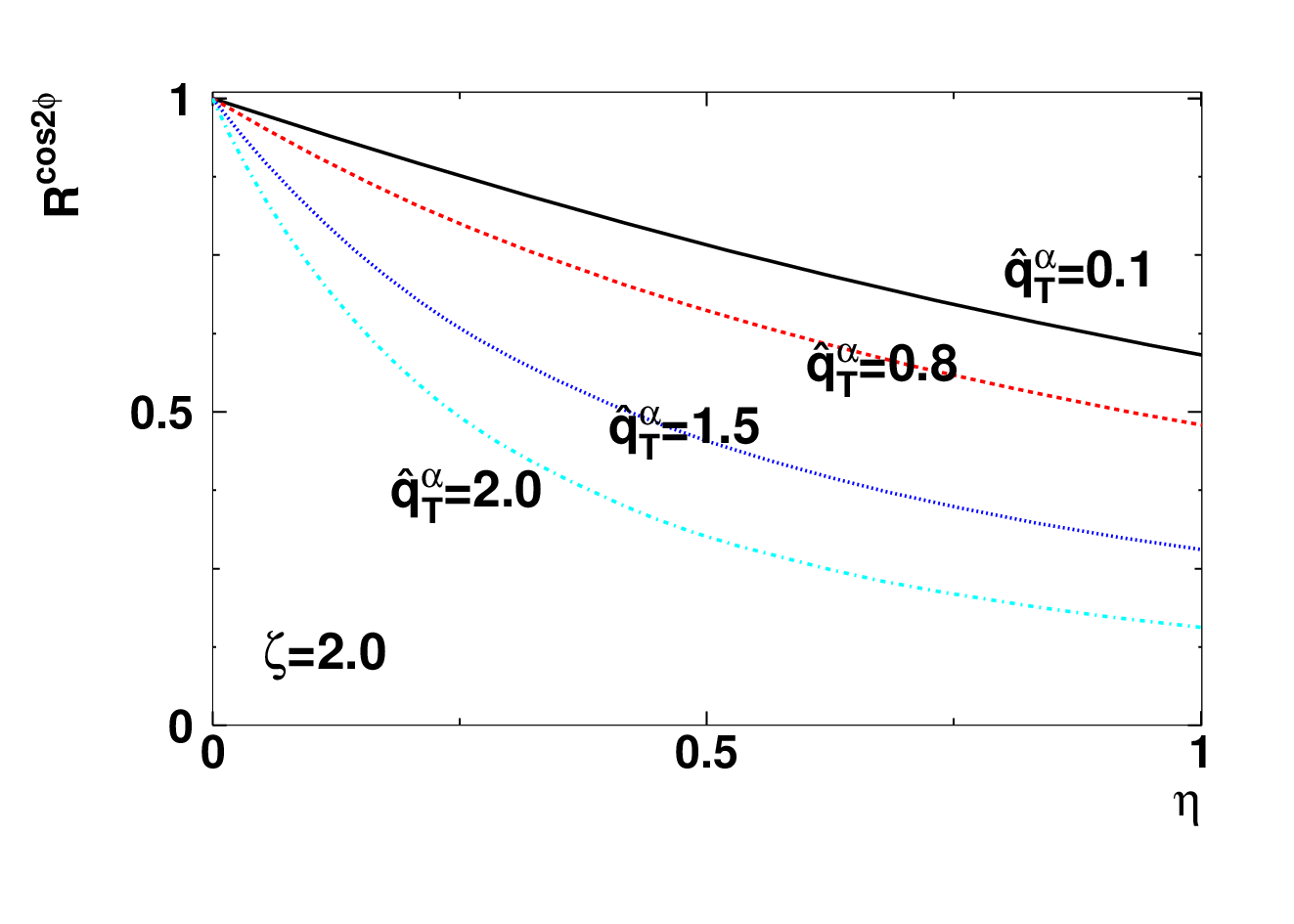
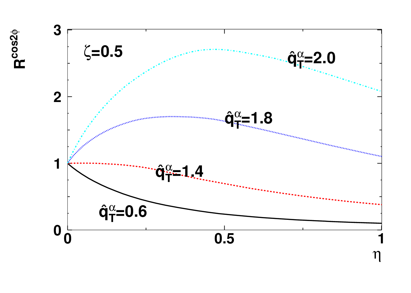
The numerical results are plotted in Fig. (1), with in panel (a) and 0.5 in panel (b), respectively, as functions of , at different scaled transverse momenta . We can see that they are very similar to the results that have been obtained in Refs. [28, 29]. In the case , the azimuthal asymmetry is suppressed and the suppression increases with the transverse momentum . When , the suppression will have the opposite dependence on . Especially, the azimuthal asymmetry could be enhanced, instead of suppression, for large enough transverse momentum . It means that the nuclear modification of the azimuthal asymmetry and its transverse momentum dependence provides a very sensitive probe to measure the width of the transverse momentum distribution in the TMD quark distribution functions. A numerical estimate of the magnitude of has been made very recently [76] by using the empirical result for the transport parameter obtained from jet quenching in cold nuclei. Here, one uses and [77, 78], and the average of the transport distance in a nucleus is . Take Au as an example, one obtains , which leads to if we choose .
We can also calculate the -integrated azimuthal asymmetry, which is given by
| (33) |
Therefore the -integrated nuclear modification factor of the azimuthal asymmetry reads
| (34) |
Now let us turn to the azimuthal asymmetries associated with the polarization of the incident nucleon, we can see four more distribution functions are involved in Eq. (4): , , and . Once more, to illustrate the nuclear dependence of all these azimuthal asymmetries resulting from these TMD distributions, we make four more Gaussian ansatz assumptions
| (35) | |||||
| (36) |
Following the same routine, we can have
| (37) | |||||
| (38) | |||||
| (39) | |||||
| (40) |
The nuclear modification factors corresponding to the above different azimuthal asymmetries are given by, respectively,
| (41) | |||||
| (42) | |||||
| (43) | |||||
| (44) |
In the special cases of and , we can reduce them to
| (45) | |||||
| (46) |
For the general cases, we can choose three independent variables for every nuclear modification factor like we did for the azimuthal asymmetry . We choose two same scaled variables and for all the nuclear modification factors, and the rest, , , and , correspond to the , , , and , respectively. With these variables, it is obvious that and are the same functions while and are the same. It should be noted that and are very similar to the result of the azimuthal asymmetry in SIDIS obtained in Ref.[28] and and are very similar to the result of the azimuthal asymmetry in SIDIS obtained in Ref. [29]. Besides, in the new scaled variables, the only difference between different azimuthal asymmetries is up to an overall factor with right power order. Because our calculation is only qualitative, we do not show their numerical results in plots one by one. The shapes and features of these azimuthal asymmetries associated with the polarization are very similar to the unpolarized azimuthal asymmetry shown in Fig. 1. The -integrated angular asymmetries can be obtained in a very straightforward way:
| (47) | |||||
| (48) | |||||
| (49) | |||||
| (50) |
It follows that the -integrated nuclear modifications of the single-spin azimuthal asymmetries read
| (51) | |||||
| (52) |
We would like to mention that, although there are not many data available, there are indeed measurements carried out on azimuthal asymmetries in DY processes with nuclear targets. There are in particular measurements on in and collisions [79, 80, 81, 82]. It is obvious that the results for the differential cross section given by Eq. (4) are applicable to reactions with pion beams as long as we drop all the polarization-dependent terms because a pion is a spin zero object. We expect formulas for similar to those given by Eqs. (27) and (28) and also a nuclear suppression effect similar to that given by Eq. (30). It is therefore clear that precise measurements of the asymmetry in these collisions will be useful not only in parameterizing Boer-Mulders function but also in studying the nuclear dependence. The accuracy of the data[79, 80, 81, 82] available is however still too low to draw any decisive judgment on the dependence of the asymmetry. Nevertheless, it is encouraging to see that such measurements can indeed be carried out and more measurements are planned [83].
IV summary
Within the framework of the TMD factorization, the nuclear dependence of the azimuthal asymmetry in polarized DY processes has been studied. We find the nuclear modifications of the azimuthal asymmetries and are the same and very similar to the azimuthal asymmetries in SIDIS obtained in Ref. [29]. The nuclear effects of the azimuthal asymmetries and are the same and similar to the azimuthal asymmetry in SIDIS obtained in Ref. [28]. Among all the azimuthal asymmetries we have considered, the nuclear dependence of the azimuthal asymmetry is most suppressed. The nuclear modification of the azimuthal asymmetry and its nontrivial transverse momentum dependence provides a very sensitive probe to measure the width of the transverse momentum distribution in the TMD quark distribution functions.
Acknowledgements.
This work is supported partially by the Major State Basic Research Development Program in China (Grant No. 2014CB845406). J.H.G. was supported in part by the National Natural Science Foundation of China under Grant No. 11105137 and the CCNU-QLPL Innovation Fund (Grant NO. QLPL2011P01 and QLPL2014P01). L.C. and Z.T.L. were supported in part by the National Natural Science Foundation of China under Grant No. 11035003.References
- [1] H. Georgi and H. Politzer, Phys. Rev. Lett. 40, 3 (1978).
- [2] R. N. Cahn, Phys. Lett. B 78, 269 (1978).
- [3] E. L. Berger, Phys. Lett. B 89, 241 (1980).
- [4] K. A. Oganesian, H. R. Avakian, N. Bianchi and P. Di Nezza, Eur. Phys. J. C 5, 681 (1998).
- [5] J. Chay and S. M. Kim, Phys. Rev. D 57, 224 (1998)
- [6] J. C. Collins and D. E. Soper, Phys. Rev. D 16, 2219 (1977).
- [7] J. C. Collins, Phys. Rev. Lett. 42, 291 (1979).
- [8] C. S. Lam and W. K. Tung, Phys. Rev. D 18, 2447 (1978).
- [9] C. S. Lam and W. -K. Tung, Phys. Lett. B 80, 228 (1979).
- [10] C. S. Lam and W. -K. Tung, Phys. Rev. D 21, 2712 (1980).
- [11] R. J. Fries, B. Muller, A. Schafer, E. Stein, Phys. Rev. Lett. 83, 4261-4264 (1999). R. J. Fries, A. Schafer, E. Stein, B. Muller, Nucl. Phys. B582, 537-570 (2000).
- [12] F. Gelis, J. Jalilian-Marian, Phys. Rev. D76, 074015 (2007).
- [13] Z. T. Liang and X. N. Wang, Phys. Rev. D 75, 094002 (2007)
- [14] J. Zhou, F. Yuan and Z. -T. Liang, Phys. Rev. D 81, 054008 (2010)
- [15] R. Baier, Y. L. Dokshitzer, A. H. Mueller, S. Peigne and D. Schiff, Nucl. Phys. B 484, 265 (1997).
- [16] G. T. Bodwin, S. J. Brodsky and G. P. Lepage, Phys. Rev. D 39, 3287 (1989).
- [17] M. Luo, J. -w. Qiu, and G. F. Sterman, Phys. Lett. B279, 377-383 (1992); Phys. Rev. D49, 4493-4502 (1994); Phys. Rev. D50, 1951-1971 (1994).
- [18] X. F. Guo, Phys. Rev. D 58, 114033 (1998).
- [19] U. A. Wiedemann, Nucl. Phys. B 588, 303 (2000)
- [20] X. -f. Guo and X. -N. Wang, Phys. Rev. Lett. 85, 3591 (2000)
- [21] X. -N. Wang and X. -f. Guo, Nucl. Phys. A 696, 788 (2001)
- [22] R. J. Fries, Phys. Rev. D 68, 074013 (2003).
- [23] A. Majumder, B. Muller, Phys. Rev. C77, 054903 (2008).
- [24] Z. T. Liang, X. N. Wang and J. Zhou, Phys. Rev. D 77, 125010 (2008)
- [25] F. D’Eramo, H. Liu and K. Rajagopal, Phys. Rev. D 84, 065015 (2011)
- [26] F. D’Eramo, H. Liu, K. Rajagopal, Nucl. Phys. A855, 457-460 (2011).
- [27] F. D’Eramo, H. Liu and K. Rajagopal, J. Phys. G 38, 124162 (2011).
- [28] J. -H. Gao, Z. -T. Liang, X. -N. Wang, Phys. Rev. C81, 065211 (2010).
- [29] Y. -K. Song, J. -H. Gao, Z. -T. Liang, X. -N. Wang, Phys. Rev. D83, 054010 (2011).
- [30] J. -H. Gao, A. Schafer and J. Zhou, Phys. Rev. D 85, 074027 (2012).
- [31] J. C. Collins and D. E. Soper, Nucl. Phys. B 193, 381 (1981) [Erratum-ibid. B 213, 545 (1983)] [Nucl. Phys. B 213, 545 (1983)].
- [32] X. -d. Ji, J. -P. Ma and F. Yuan, Phys. Lett. B 597, 299 (2004)
- [33] D. Boer, Phys. Rev. D 60, 014012 (1999)
- [34] S. Arnold, A. Metz and M. Schlegel, Phys. Rev. D 79, 034005 (2009)
- [35] Z. Lu, B. -Q. Ma and J. Zhu, Phys. Rev. D 84, 074036 (2011)
- [36] P. J. Mulders and R. D. Tangerman, Nucl. Phys. B 461, 197 (1996) [Erratum-ibid. B 484, 538 (1997)]
- [37] K. Goeke, A. Metz and M. Schlegel, Phys. Lett. B 618, 90 (2005)
- [38] A. Bacchetta, M. Diehl, K. Goeke, A. Metz, P. J. Mulders and M. Schlegel, JHEP 0702, 093 (2007)
- [39] D. W. Sivers, Phys. Rev. D 41, 83 (1990).
- [40] D. W. Sivers, Phys. Rev. D 43, 261 (1991).
- [41] D. Boer and P. J. Mulders, Phys. Rev. D 57, 5780 (1998)
- [42] B. Pasquini, M. Pincetti and S. Boffi, Phys. Rev. D 76, 034020 (2007).
- [43] M. Anselmino, M. Boglione, U. D’Alesio, A. Kotzinian, F. Murgia, A. Prokudin and C. Turk, Phys. Rev. D 75, 054032 (2007).
- [44] M. Anselmino, M. Boglione, U. D’Alesio, A. Kotzinian, F. Murgia, A. Prokudin and S. Melis, Nucl. Phys. Proc. Suppl. 191, 98 (2009).
- [45] L. P. Gamberg, G. R. Goldstein and K. A. Oganessyan, Phys. Rev. D 67, 071504(R) (2003).
- [46] L. P. Gamberg, G. R. Goldstein and M. Schlegel, Phys. Rev. D 77, 094016 (2008).
- [47] A. Bacchetta, L.P. Gamberg, G.R. Goldstein, A. Mukherjee, Phys. Lett. B 659, 234 (2008).
- [48] H. Avakian, S. J. Brodsky, A. Deur and F. Yuan, Phys. Rev. Lett. 99, 082001 (2007).
- [49] B. Pasquini, S. Cazzaniga and S. Boffi, Phys. Rev. D 78, 034025 (2008).
- [50] A. Bacchetta, F. Conti and M. Radici, Phys. Rev. D 78, 074010 (2008).
- [51] A. Courtoy, F. Fratini, S. Scopetta and V. Vento, Phys. Rev. D 78 (2008) 034002.
- [52] A. Courtoy, S. Scopetta and V. Vento, Phys. Rev. D 79, 074001 (2009).
- [53] A. Courtoy, S. Scopetta and V. Vento, Phys. Rev. D 80, 074032 (2009).
- [54] H. Avakian, A. V. Efremov, P. Schweitzer and F. Yuan, Phys. Rev. D 78, 114024 (2008).
- [55] M. Anselmino et al., Eur. Phys. J. A 39 (2009) 89; M. Anselmino, M. Boglione, U. D’Alesio, A. Kotzinian, F. Murgia and A. Prokudin, Phys. Rev. D 71, 074006 (2005); M. Anselmino, M. Boglione, U. D’Alesio, A. Kotzinian, F. Murgia and A. Prokudin, Phys. Rev. D 72, 094007 (2005) [Erratum-ibid. D 72, 099903 (2005)];
- [56] S. Arnold, A. V. Efremov, K. Goeke, M. Schlegel and P. Schweitzer, arXiv:0805.2137 [hep-ph].
- [57] A. V. Efremov, P. Schweitzer, O. V. Teryaev and P. Zavada, Phys. Rev. D 80, 014021 (2009).
- [58] J. She, J. Zhu and B. Q. Ma, Phys. Rev. D 79, 054008 (2009).
- [59] R. Jakob, P. J. Mulders and J. Rodrigues, Nucl. Phys. A 626, 937 (1997);
- [60] A. V. Efremov, K. Goeke and P. Schweitzer, Eur. Phys. J. C 32, 337 (2003).
- [61] F. Yuan, Phys. Lett. B 575, 45 (2003).
- [62] P. V. Pobylitsa, arXiv:hep-ph/0301236.
- [63] A. V. Efremov, K. Goeke and P. Schweitzer, Eur. Phys. J. C 35, 207 (2004).
- [64] B. Pasquini and F. Yuan, Phys. Rev. D 81, 114013 (2010)
- [65] J. C. Collins, Nucl. Phys. B 396, 161 (1993)
- [66] Z. -T. Liang and T. -C. Meng, Z. Phys. A 344, 171 (1992); C. Boros, Z. T. Liang and T. C. Meng, Phys. Rev. Lett. 70, 1751 (1993).
- [67] S. J. Brodsky, D. S. Hwang and I. Schmidt, Nucl. Phys. B 642, 344 (2002)
- [68] H. Mkrtchyan, P. E. Bosted, G. S. Adams, A. Ahmidouch, T. Angelescu, J. Arrington, R. Asaturyan and O. K. Baker et al., Phys. Lett. B 665, 20 (2008)
- [69] A. Airapetian et al. [HERMES Collaboration], Phys. Rev. Lett. 103, 152002 (2009)
- [70] H. Avakian et al. [CLAS Collaboration], Phys. Rev. Lett. 105, 262002 (2010)
- [71] M. G. Alekseev et al. [COMPASS Collaboration], Phys. Lett. B 692, 240 (2010)
- [72] J. C. Collins, A. V. Efremov, K. Goeke, M. Grosse Perdekamp, S. Menzel, B. Meredith, A. Metz and P. Schweitzer, Phys. Rev. D 73, 094023 (2006)
- [73] W. Vogelsang and F. Yuan, Phys. Rev. D 72, 054028 (2005)
- [74] A. Majumder, R. J. Fries and B. Muller, Phys. Rev. C 77, 065209 (2008)
- [75] A. Schafer and J. Zhou, Phys. Rev. D 88, 074012 (2013)
- [76] Y. -k. Song, Z. -t. Liang and X. -N. Wang, arXiv:1402.3042 [nucl-th].
- [77] W. -t. Deng and X. -N. Wang, Phys. Rev. C 81, 024902 (2010)
- [78] N. -B. Chang, W. -T. Deng and X. -N. Wang, arXiv:1401.5109 [nucl-th].
- [79] J. Badier et al. [NA3 Collaboration], Z. Phys. C 11, 195 (1981).
- [80] J. S. Conway, C. E. Adolphsen, J. P. Alexander, K. J. Anderson, J. G. Heinrich, J. E. Pilcher, A. Possoz and E. I. Rosenberg et al., Phys. Rev. D 39, 92 (1989).
- [81] M. Guanziroli et al. [NA10 Collaboration], Z. Phys. C 37, 545 (1988).
- [82] S. Falciano et al. [NA10 Collaboration], Z. Phys. C 31, 513 (1986).
- [83] See e.g., W. -C. Chang and D. Dutta, Int. J. Mod. Phys. E 22, 1330020 (2013), and references therein.