跳到论文正文
W Papers独立论文阅读器 arXiv:1308.3643 论文正文 计算阅读时间 · 0%
引用这篇论文根据当前论文元数据生成,正式投稿前建议核对。


License: arXiv.org perpetual non-exclusive license
arXiv:1308.3643v1 [math.NA] 16 Aug 2013

Robust boundary tracking for reachable sets of nonlinear differential inclusions

Janosch Rieger Note: Institut für Mathematik, Universität Frankfurt, Postfach 111932, D-60054 Frankfurt a.M., Germany; phone: +49/69/798-22715, fax: +49/69/798-28846.
August 24, 2026
Abstract

The Euler scheme is up to date the most important numerical method for ordinary differential inclusions, because the use of the available higher-order methods is prohibited by their enormous complexity after spatial discretization. Therefore, it makes sense to reassess the Euler scheme and optimize its performance. In the present paper, a considerable reduction of the computational cost is achieved by setting up a numerical method that computes the boundaries instead of the complete reachable sets of the fully discretized Euler scheme from lower-dimensional data only. Rigorous proofs for the propriety of this method are given, and numerical examples illustrate the gain of computational efficiency as well as the robustness of the scheme against changes of topology of the reachable sets.

Keywords: differential inclusion, numerical method, reachable sets.

AMS subject classifications: 34A60, 65L20.

1 Introduction

Consider the differential inclusion

x′​(t)∈F⁡(t,x⁡(t)),x⁡(0)∈X0,x^{\prime}(t)\in F(t,x(t)),\quad x(0)\in X_{0}, (1)

where F:ℝ×ℝd⇉ℝdF:\mathbbm{R}\times\mathbbm{R}^{d}\rightrightarrows\mathbbm{R}^{d} is a Lipschitz continuous multivalued mapping that assigns to each pair (t,x)∈ℝ×ℝd(t,x)\in\mathbbm{R}\times\mathbbm{R}^{d} a convex and compact subset of ℝd\mathbbm{R}^{d}. Differential inclusions model global aspects of control and deterministic uncertainty. In a sense, they are the deterministic counterpart of stochastic differential equations. The reachable sets

ℛ⁡(T,X0)={x⁡(T):x⁡(⋅)​solves (1)}\mathcal{R}(T,X_{0})=\{x(T):x(\cdot)\ \text{solves \eqref{odi}}\}

are of considerable interest, because they are the sets of all states that can be reached using admissible controls or perturbations. The theory of differential inclusions is well-developed, and the reader is referred to the monographs [1] and [6] for details.

The numerical approximation of the set of all solutions of (1) and the corresponding reachable sets remains a challenging subject even in the low-dimensional context, because it is massively affected by the curse of dimensionality. This paper is concerned with the multivalued Euler scheme

Φ:ℝ×ℝd⇉ℝd,Φ⁡(x)=x+h​F​(t,x)\Phi:\mathbbm{R}\times\mathbbm{R}^{d}\rightrightarrows\mathbbm{R}^{d},\quad\Phi(x)=x+hF(t,x)

for differential inclusions of form (1) that has been investigated in [7] and several papers since. The reachable set ℛ⁡(T,X0)\mathcal{R}(T,X_{0}) can be approximated by fixing some N∈ℕN\in\mathbbm{N} and h>0h>0 such that T=N​hT=Nh and computing

ℛh(tn+1,X0)=Φ(tn,ℛh(tn,X0)),n=0,…,N−1,ℛh(t0,X0)=X0\mathcal{R}_{h}(t_{n+1},X_{0})=\Phi(t_{n},\mathcal{R}_{h}(t_{n},X_{0})),\ n=0,\ldots,N-1,\quad\mathcal{R}_{h}(t_{0},X_{0})=X_{0}

recursively, where tn=n​ht_{n}=nh. For practical computations, it is necessary to discretize these sets. This is usually done by introducing a grid Δρ=ρ​ℤd\Delta_{\rho}=\rho\mathbbm{Z}^{d} and a fully discrete Euler scheme

Φ~α:ℝ×Δρ⇉Δρ,Φ~α​(x)=Bα​(Φ⁡(x))∩Δρ,ℛ~h​(t0,X0)=Bα​(X0)∩Δρ\displaystyle\tilde{\Phi}_{\alpha}:\mathbbm{R}\times\Delta_{\rho}\rightrightarrows\Delta_{\rho},\quad\tilde{\Phi}_{\alpha}(x)=B_{\alpha}(\Phi(x))\cap\Delta_{\rho},\quad\tilde{\mathcal{R}}_{h}(t_{0},X_{0})=B_{\alpha}(X_{0})\cap\Delta_{\rho}
ℛ~h(tn+1,X0)=Φ~α(tn,ℛ~h(tn,X0)),n=0,…,N−1.\displaystyle\tilde{\mathcal{R}}_{h}(t_{n+1},X_{0})=\tilde{\Phi}_{\alpha}(t_{n},\tilde{\mathcal{R}}_{h}(t_{n},X_{0})),\ n=0,\ldots,N-1.

for some α≥ρ/2\alpha\geq\rho/2, because this setting guarantees that Φ~α​(⋅)\tilde{\Phi}_{\alpha}(\cdot) is a good approximation of Φ⁡(⋅)\Phi(\cdot). Spatial discretization and its impact on error estimates have been discussed in [4].

The computation of reachable sets by the fully discrete Euler scheme is very costly, which is mainly due to the fact that the images Φ~α​(x)\tilde{\Phi}_{\alpha}(x) and Φ~α​(x~)\tilde{\Phi}_{\alpha}(\tilde{x}) overlap if xx and x~\tilde{x} are close to each other and the computed information is highly redundant. Several attempts have been made to develop faster numerical methods.

In [9] and [13], a multivalued version of Heun’s method and more general Runge-Kutta methods are shown to converge quadratically w.r.t. the time-step under strong assumptions on FF when considered without spatial discretization. Successive evaluations of the discretized multivalued right-hand sides, however, are so costly that in practice, the performance of such methods is worse than that of the Euler scheme.

The paper [12] investigates the properties of the Euler scheme for differential inclusions with non-convex right-hand sides and, in particular, proves first-order convergence in this situation. As the closures of the reachable sets of a differential inclusion with non-convex right-hand side coincide with the reachable sets of the convexified problem, this result demonstrates that it is possible to approximate the desired sets using only extremal points of the right-hand sides for computing the Euler step without losing the order of convergence. Nevertheless, the resulting version of the Euler scheme has a larger error than its classical pendant, so that the gain of efficiency is moderate.

An unconventional approach to the problem has recently been published in [3], where the defining relations of the Euler or a more general Runge-Kutta scheme are considered as constraints in an optimization routine that aims to minimize the distance between given points in phase space and the states that can be reached by trajectories of the numerical scheme. This method reduces unnecessary computations efficiently, but bears the risk of losing parts of the reachable set by failure of the optimizer to find the global minimum.

The boundary Euler method proposed and analyzed in the present paper uses a simple but effective strategy to reduce computational costs. It tracks the boundaries (precise definition in Section 3) of the reachable sets of the fully discretized Euler scheme instead of computing the whole reachable sets and computes a second layer of exterior points close to the boundary in every time-step from a layer of exterior points in the preimage. The boundary and the exterior layer together contain all necessary information about the topology of the discrete reachable sets. Moreover, the algorithm can be arranged in such a way that instead of full images F⁡(⋅)F(\cdot) it is essentially sufficient to work with the boundary ∂F⁡(⋅)\partial F(\cdot) of the right-hand side. As the boundary of the fully discrete Euler scheme is exactly reproduced, the boundary Euler scheme satisfies the same error estimates.

It is surprisingly hard to prove that the boundary Euler method indeed computes the boundaries of the discrete reachable sets. To this end, Section 2 gathers some analytical prerequisites and Section 3 exploits them to set up a preliminary version of the method. The drawback of this preliminary version is that full images F⁡(⋅)F(\cdot) of the right-hand side have to be computed in order to ensure the propriety of the algorithm. Nontrivial topological arguments given in Section 4 improve the results of Section 2 and facilitate the formulation of the boundary Euler method in its final form.

The boundary Euler scheme is at present the fastest numerical method for non-stiff ordinary differential inclusions. Up to our knowledge, the result as well as some of the technical tools necessary for the proof have never been considered in the literature. Throughout the paper, great care is taken to obtain optimal constants, because suboptimal constants strongly increase the computational costs of the boundary Euler method without increasing its precision.

2 Notation and analytical prerequisites

The notation used in this paper is mostly standard. For any set A⊂ℝdA\subset\mathbbm{R}^{d}, the symbols AcA^{c}, int⁡A\interior A, and ∂A\partial A denote the complement, the interior, and the boundary of AA. For p∈[1,∞]p\in[1,\infty], the one-sided and the symmetric Hausdorff distances (induced by the pp-norm) between compact sets A,B⊂ℝdA,B\subset\mathbbm{R}^{d} are given by dist⁡(A,B)p:=supa∈Ainfb∈B|a−b|p\dist(A,B)_{p}:=\sup_{a\in A}\inf_{b\in B}|a-b|_{p} and distH⁡(A,B)p:=max⁡{dist⁡(A,B)p,dist⁡(B,A)p}\dist_{H}(A,B)_{p}:=\max\{\dist(A,B)_{p},\dist(B,A)_{p}\}. For any x∈ℝdx\in\mathbbm{R}^{d}, we set Proj⁡(x,A)p:={a∈A:|x−a|p=dist⁡(x,A)p}\Proj(x,A)_{p}:=\{a\in A:|x-a|_{p}=\dist(x,A)_{p}\}, and for r≥0r\geq 0 we define Br​(A)p:={x∈ℝd:dist⁡(x,A)p≤r}B_{r}(A)_{p}:=\{x\in\mathbbm{R}^{d}:\dist(x,A)_{p}\leq r\}.

Let F:ℝd1⇉ℝd2F:\mathbbm{R}^{d_{1}}\rightrightarrows\mathbbm{R}^{d_{2}} be a set-valued mapping with compact images. Then F⁡(⋅)F(\cdot) is called LL-Lipschitz if distH⁡(F⁡(x),F⁡(x~))p≤L​|x−x~|p\dist_{H}(F(x),F(\tilde{x}))_{p}\leq L|x-\tilde{x}|_{p} for all x,x~∈ℝd1x,\tilde{x}\in\mathbbm{R}^{d_{1}}. Let 𝒞​𝒞​(ℝd)\mathcal{CC}(\mathbbm{R}^{d}) denote the collection of all subsets of ℝd\mathbbm{R}^{d} that are convex and compact. It is well-known that a mapping F:ℝd1→𝒞​𝒞​(ℝd2)F:\mathbbm{R}^{d_{1}}\rightarrow\mathcal{CC}(\mathbbm{R}^{d_{2}}) is Lipschitz if and only if its boundary ∂F⁡(⋅)\partial F(\cdot) is Lipschitz with the same Lipschitz constant (see [10]).

The identity mapping is denoted i​d:ℝd→ℝdid:\mathbbm{R}^{d}\rightarrow\mathbbm{R}^{d}. For any two paths φ,~​φ∈C⁡([0,1],ℝd)\varphi,\tilde{}\varphi\in C([0,1],\mathbbm{R}^{d}) with φ⁡(1)=~​φ​(0)\varphi(1)=\tilde{}\varphi(0), their concatenation ~​φ∘φ∈C⁡([0,1],ℝd)\tilde{}\varphi\circ\varphi\in C([0,1],\mathbbm{R}^{d}) is defined by

(~​φ∘φ)​(λ):={φ⁡(2⋅λ),0≤λ≤1/2,~​φ​(2⋅λ−1),1/2≤λ≤1.(\tilde{}\varphi\circ\varphi)(\lambda):=\left\{\begin{array}[]{ll}\varphi(2\cdot\lambda),&0\leq\lambda\leq 1/2,\\ \tilde{}\varphi(2\cdot\lambda-1),&1/2\leq\lambda\leq 1.\end{array}\right.

The following result is related to [5, Theorem 2], where more general mappings are discussed in the Euclidean ℝd\mathbbm{R}^{d}. For the purposes of the present paper, however, it will be essential to measure distances in |⋅|∞|\cdot|_{\infty}. An error term of size d\sqrt{d} caused by embedding (ℝd,|⋅|2)(\mathbbm{R}^{d},|\cdot|_{2}) into (ℝd,|⋅|∞)(\mathbbm{R}^{d},|\cdot|_{\infty}) is not tolerable, because suboptimal estimates force the algorithm to carry out unnecessary computations.

Proposition 1.

Let G:ℝd→𝒞​𝒞​(ℝd)G:\mathbbm{R}^{d}\rightarrow\mathcal{CC}(\mathbbm{R}^{d}) be ll-Lipschitz w.r.t. |⋅|∞|\cdot|_{\infty} with l<1l<1. Then for any x0,y^∈ℝdx^{0},\hat{y}\in\mathbbm{R}^{d} there exists x^∈ℝd\hat{x}\in\mathbbm{R}^{d} such that y^∈x^+G⁡(x^)\hat{y}\in\hat{x}+G(\hat{x}) and

|x0−x^|∞≤dist⁡(y^,x0+G⁡(x0))∞1−l.|x^{0}-\hat{x}|_{\infty}\leq\frac{\dist(\hat{y},x^{0}+G(x^{0}))_{\infty}}{1-l}. (2)

If y^∉x0+G⁡(x0)\hat{y}\notin x^{0}+G(x^{0}), then there exists x^\hat{x} satisfying (2) and y^∈x^+∂G⁡(x^)\hat{y}\in\hat{x}+\partial G(\hat{x}).

Proof.

Construct successively

gk∈Proj⁡(y^−xk,G⁡(xk))∞,rk:=y^−(xk+gk),xk+1:=xk+rk\displaystyle g^{k}\in\Proj(\hat{y}-x^{k},G(x^{k}))_{\infty},\quad r^{k}:=\hat{y}-(x^{k}+g^{k}),\quad x^{k+1}:=x^{k}+r^{k}

for k∈ℕk\in\mathbbm{N}. Then

|rk+1|∞\displaystyle|r^{k+1}|_{\infty} =dist⁡(y^,xk+1+G⁡(xk+1))∞=dist⁡(y^,xk+rk+G⁡(xk+1))∞\displaystyle=\dist(\hat{y},x^{k+1}+G(x^{k+1}))_{\infty}=\dist(\hat{y},x^{k}+r^{k}+G(x^{k+1}))_{\infty}
=dist⁡(gk,G⁡(xk+1))∞≤dist⁡(G⁡(xk),G⁡(xk+1))∞\displaystyle=\dist(g^{k},G(x^{k+1}))_{\infty}\leq\dist(G(x^{k}),G(x^{k+1}))_{\infty}
≤l​|xk+1−xk|∞≤l​|rk|∞\displaystyle\leq l|x^{k+1}-x^{k}|_{\infty}\leq l|r^{k}|_{\infty}

for k∈ℕk\in\mathbbm{N}. Hence

|xn−xm|∞≤∑k=mn−1|rk|∞≤|r0|∞​∑k=mn−1lk≤lm1−l​|r0|∞|x^{n}-x^{m}|_{\infty}\leq\sum_{k=m}^{n-1}|r^{k}|_{\infty}\leq|r^{0}|_{\infty}\sum_{k=m}^{n-1}l^{k}\leq\frac{l^{m}}{1-l}|r^{0}|_{\infty}

for all m,n∈ℕm,n\in\mathbbm{N} with m≤nm\leq n, so that {xk}k=0∞\{x^{k}\}_{k=0}^{\infty} is Cauchy and x^:=limk→∞xk\hat{x}:=\lim_{k\rightarrow\infty}x^{k} exists. Then

|x^−x0|∞≤∑k=0∞|rk|∞≤|r0|∞1−l=dist⁡(y^,x0+G⁡(x0))∞1−l,|\hat{x}-x^{0}|_{\infty}\leq\sum_{k=0}^{\infty}|r^{k}|_{\infty}\leq\frac{|r^{0}|_{\infty}}{1-l}=\frac{\dist(\hat{y},x^{0}+G(x^{0}))_{\infty}}{1-l},

and

dist⁡(y^,x^+G⁡(x^))∞=limk→∞dist⁡(y^,xk+G⁡(xk))∞=limk→∞|rk|∞=0\dist(\hat{y},\hat{x}+G(\hat{x}))_{\infty}=\lim_{k\rightarrow\infty}\dist(\hat{y},x^{k}+G(x^{k}))_{\infty}=\lim_{k\rightarrow\infty}|r^{k}|_{\infty}=0

together with G⁡(x^)∈𝒞​𝒞​(ℝd)G(\hat{x})\in\mathcal{CC}(\mathbbm{R}^{d}) imply y^∈x^+G⁡(x^)\hat{y}\in\hat{x}+G(\hat{x}).

Consider the case y^∉x0+G⁡(x0)\hat{y}\notin x^{0}+G(x^{0}). Construct x^∈ℝd\hat{x}\in\mathbbm{R}^{d} with y^∈x^+G⁡(x^)\hat{y}\in\hat{x}+G(\hat{x}) and (2) as above. Define φ⁡(λ):=λ​x^+(1−λ)​x0\varphi(\lambda):=\lambda\hat{x}+(1-\lambda)x^{0} for λ∈[0,1]\lambda\in[0,1]. Let

λ∗:=inf{λ∈[0,1]:y^∈φ⁡(λ)+G⁡(φ⁡(λ))}.\lambda^{*}:=\inf\{\lambda\in[0,1]:\hat{y}\in\varphi(\lambda)+G(\varphi(\lambda))\}.

There exists a sequence (λn)n∈ℕ⊂[0,1](\lambda_{n})_{n\in\mathbbm{N}}\subset[0,1] with λn↘λ∗\lambda_{n}\searrow\lambda^{*} and y^∈φ⁡(λn)+G⁡(φ⁡(λn))\hat{y}\in\varphi(\lambda_{n})+G(\varphi(\lambda_{n})), so that by continuity y^∈φ⁡(λ∗)+G⁡(φ⁡(λ∗))\hat{y}\in\varphi(\lambda^{*})+G(\varphi(\lambda^{*})).

Assume that y^∈φ⁡(λ∗)+int⁡G⁡(φ⁡(λ∗))\hat{y}\in\varphi(\lambda^{*})+\interior G(\varphi(\lambda^{*})). Then the properties of GG ensure that there exists ε>0\varepsilon>0 such that

y^∈φ⁡(λ)+G⁡(φ⁡(λ))for all​λ∈(λ∗−ε,λ∗+ε),\hat{y}\in\varphi(\lambda)+G(\varphi(\lambda))\quad\text{for all}\ \lambda\in(\lambda^{*}-\varepsilon,\lambda^{*}+\varepsilon), (3)

which contradicts minimality of λ∗\lambda^{*}. Hence y^∈φ⁡(λ∗)+∂G⁡(φ⁡(λ∗))\hat{y}\in\varphi(\lambda^{*})+\partial G(\varphi(\lambda^{*})), and by construction φ⁡(λ∗)\varphi(\lambda^{*}) satisfies (2). ∎

Obviously, the (time-independent) Euler map Φ⁡(x)=x+h​F​(x)\Phi(x)=x+hF(x) satisfies the assumptions of Proposition 1 if F:ℝd→𝒞​𝒞​(ℝd)F:\mathbbm{R}^{d}\rightarrow\mathcal{CC}(\mathbbm{R}^{d}) is LL-Lipschitz and L​h<1Lh<1.

Remark 2.

The fact that GG has convex images is only used in (3). One could think of weaker assumptions such as ll-Lipschitz continuity of a compact-valued mapping G:ℝd⇉ℝdG:\mathbbm{R}^{d}\rightrightarrows\mathbbm{R}^{d} and continuity of the complement Gc:ℝd⇉ℝdG^{c}:\mathbbm{R}^{d}\rightrightarrows\mathbbm{R}^{d} to prevent the sudden formation of holes. This is, however, not the focus of this paper.

In the following proposition, it is again important to work in the maximum norm to avoid embedding constants that may lead to unnecessary restrictions of the step size hh.

Proposition 3.

Let G:ℝd→𝒞​𝒞​(ℝd)G:\mathbbm{R}^{d}\rightarrow\mathcal{CC}(\mathbbm{R}^{d}) be ll-Lipschitz w.r.t. |⋅|∞|\cdot|_{\infty} with l<1l<1. Then for any ξ∈ℝd\xi\in\mathbbm{R}^{d} the set (id+G)−1​(ξ):={x∈ℝd:ξ∈x+G⁡(x)}(\id+G)^{-1}(\xi):=\{x\in\mathbbm{R}^{d}:\xi\in x+G(x)\} is nonempty and path-connected.

Proof.

By Proposition 1 we have (id+G)−1​(ξ)≠∅(\id+G)^{-1}(\xi)\neq\emptyset. Let z,z~∈(id+G)−1​(ξ)z,\tilde{z}\in(\id+G)^{-1}(\xi). Define x0:[0,1]→ℝdx^{0}:[0,1]\rightarrow\mathbbm{R}^{d} by

x0​(λ):=λ​z+(1−λ)​z~.x^{0}(\lambda):=\lambda z+(1-\lambda)\tilde{z}.

For k∈ℕk\in\mathbbm{N} set p⁡(k):=k2+2p(k):=k^{2}+2 and define successively functions fk,rk,xk+1:[0,1]→ℝdf^{k},r^{k},x^{k+1}:[0,1]\rightarrow\mathbbm{R}^{d} by

gk​(λ)\displaystyle g^{k}(\lambda) :=Proj(ξ−xk(λ),G(xk(λ))))p⁡(k),\displaystyle:=\Proj(\xi-x^{k}(\lambda),G(x^{k}(\lambda))))_{p(k)},
rk​(λ)\displaystyle r^{k}(\lambda) :=ξ−(xk​(λ)+gk​(λ)),\displaystyle:=\xi-(x^{k}(\lambda)+g^{k}(\lambda)),
xk+1​(λ)\displaystyle x^{k+1}(\lambda) :=xk​(λ)+rk​(λ),\displaystyle:=x^{k}(\lambda)+r^{k}(\lambda),

where Proj⁡(⋅,⋅)p\Proj(\cdot,\cdot)_{p} denotes the projection w.r.t. |⋅|p|\cdot|_{p}. These functions are continuous, because (ℝd,|⋅|p)(\mathbbm{R}^{d},|\cdot|_{p}) is strictly convex for 1<p<∞1<p<\infty (see [2, Section 9.3]). Moreover, xk​(0)=zx^{k}(0)=z and xk​(1)=z~x^{k}(1)=\tilde{z} hold for all k∈ℕk\in\mathbbm{N}, and gk​(λ)∈G⁡(xk​(λ))g^{k}(\lambda)\in G(x^{k}(\lambda)) for all λ∈[0,1]\lambda\in[0,1] and k∈ℕk\in\mathbbm{N}.

Since λ↦dist⁡(ξ,x0​(λ)+G⁡(x0​(λ)))∞\lambda\mapsto\dist(\xi,x^{0}(\lambda)+G(x^{0}(\lambda)))_{\infty} is a continuous function from the compact interval [0,1][0,1] to the real numbers, ‖r0‖∞<∞\|r^{0}\|_{\infty}<\infty. In addition,

|rk+1​(λ)|∞≤|rk+1​(λ)|p⁡(k+1)=dist⁡(ξ,xk+1​(λ)+G⁡(xk+1​(λ)))p⁡(k+1)\displaystyle|r^{k+1}(\lambda)|_{\infty}\leq|r^{k+1}(\lambda)|_{p(k+1)}=\dist(\xi,x^{k+1}(\lambda)+G(x^{k+1}(\lambda)))_{p(k+1)}
=dist⁡(gk​(λ),G⁡(xk+1​(λ)))p⁡(k+1)≤dist⁡(G⁡(xk​(λ)),G⁡(xk+1​(λ)))p⁡(k+1)\displaystyle=\dist(g^{k}(\lambda),G(x^{k+1}(\lambda)))_{p(k+1)}\leq\dist(G(x^{k}(\lambda)),G(x^{k+1}(\lambda)))_{p(k+1)}
≤d1p⁡(k+1)​dist⁡(G⁡(xk​(λ)),G⁡(xk+1​(λ)))∞≤d1p⁡(k+1)​l|rk​(λ)|∞,\displaystyle\leq d^{\frac{1}{p(k+1)}}\dist(G(x^{k}(\lambda)),G(x^{k+1}(\lambda)))_{\infty}\leq d^{\frac{1}{p(k+1)}}l|r^{k}(\lambda)|_{\infty},

so that

‖rk‖∞\displaystyle\|r^{k}\|_{\infty} ≤(∏j=1kd1p⁡(j))​lk​‖r0‖∞≤(∏j=1kd1j2)​lk​‖r0‖∞\displaystyle\leq(\prod_{j=1}^{k}d^{\frac{1}{p(j)}})l^{k}\|r^{0}\|_{\infty}\leq(\prod_{j=1}^{k}d^{\frac{1}{j^{2}}})l^{k}\|r^{0}\|_{\infty}
=d∑j=1k1j2​lk​‖r0‖∞≤dπ26​lk​‖r0‖∞.\displaystyle=d^{\sum_{j=1}^{k}\frac{1}{j^{2}}}l^{k}\|r^{0}\|_{\infty}\leq d^{\frac{\pi^{2}}{6}}l^{k}\|r^{0}\|_{\infty}.

For m,n∈ℕm,n\in\mathbbm{N} with m≤nm\leq n, it follows that

‖xn−xm‖∞\displaystyle\|x^{n}-x^{m}\|_{\infty} ≤∑k=mn−1‖rk‖∞≤dπ26​‖r0‖∞​∑k=mn−1lk≤dπ26​‖r0‖∞​lm1−l.\displaystyle\leq\sum_{k=m}^{n-1}\|r^{k}\|_{\infty}\leq d^{\frac{\pi^{2}}{6}}\|r^{0}\|_{\infty}\sum_{k=m}^{n-1}l^{k}\leq d^{\frac{\pi^{2}}{6}}\|r^{0}\|_{\infty}\frac{l^{m}}{1-l}.

Hence {xk}k=0∞⊂(C([0,1],ℝd),∥⋅∥∞)\{x^{k}\}_{k=0}^{\infty}\subset(C([0,1],\mathbbm{R}^{d}),\|\cdot\|_{\infty}) is Cauchy, and there exists x^∈C⁡([0,1],ℝd)\hat{x}\in C([0,1],\mathbbm{R}^{d}) with limk→∞‖xk−x^‖∞=0\lim_{k\rightarrow\infty}\|x^{k}-\hat{x}\|_{\infty}=0. It is clear that x^​(0)=z\hat{x}(0)=z and x^​(1)=z~\hat{x}(1)=\tilde{z}. Finally,

0←d1p⁡(k)​‖rk‖∞\displaystyle 0\leftarrow d^{\frac{1}{p(k)}}\|r^{k}\|_{\infty} ≥‖rk‖p⁡(k)=dist⁡(ξ,(id+G)​(xk​(λ)))p⁡(k)\displaystyle\geq\|r^{k}\|_{p(k)}=\dist(\xi,(\id+G)(x^{k}(\lambda)))_{p(k)}
≥dist⁡(ξ,(id+G)​(xk​(λ)))∞→dist⁡(ξ,(id+G)​(x^​(λ)))∞\displaystyle\geq\dist(\xi,(\id+G)(x^{k}(\lambda)))_{\infty}\rightarrow\dist(\xi,(\id+G)(\hat{x}(\lambda)))_{\infty}

for k→∞k\rightarrow\infty implies ξ∈(id+G)​(x^​(λ))\xi\in(\id+G)(\hat{x}(\lambda)) for all λ∈[0,1]\lambda\in[0,1]. ∎

The following observation is the main motivation for the development of the boundary Euler method.

Proposition 4.

Let F:ℝd→𝒞​𝒞​(ℝd)F:\mathbbm{R}^{d}\rightarrow\mathcal{CC}(\mathbbm{R}^{d}) be LL-Lipschitz, let h>0h>0 be so small that L​h<1Lh<1, and let M⊂ℝdM\subset\mathbbm{R}^{d} be compact.

  • a)

    If x∈Mx\in M and δ:=dist⁡(x,∂M)∞>0\delta:=\dist(x,\partial M)_{\infty}>0, then

    B(1−L​h)​δ​(Φ⁡(x))∞⊂Φ⁡(M)B_{(1-Lh)\delta}(\Phi(x))_{\infty}\subset\Phi(M)
  • b)

    For every y∈∂(Φ⁡(M))y\in\partial(\Phi(M)), we have ∅≠Φ−1​(y)∩M⊂∂M\emptyset\neq\Phi^{-1}(y)\cap M\subset\partial M, and for every x∈∂Mx\in\partial M with y∈Φ⁡(x)y\in\Phi(x) we have y∈∂Φ⁡(x)y\in\partial\Phi(x).

Proof.
  • a)

    Let y∈Φ⁡(x)y\in\Phi(x) and y~∈B(1−L​h)​δ​(y)∞\tilde{y}\in B_{(1-Lh)\delta}(y)_{\infty}. By Proposition 1, there exists x~∈ℝd\tilde{x}\in\mathbbm{R}^{d} such that y~∈Φ⁡(x~)\tilde{y}\in\Phi(\tilde{x}) and

    |x~−x|∞≤dist⁡(y~,Φ⁡(x))∞1−L​h≤|y~−y|∞1−L​h≤δ,|\tilde{x}-x|_{\infty}\leq\frac{\dist(\tilde{y},\Phi(x))_{\infty}}{1-Lh}\leq\frac{|\tilde{y}-y|_{\infty}}{1-Lh}\leq\delta,

    so that x~∈M\tilde{x}\in M and y~∈Φ⁡(M)\tilde{y}\in\Phi(M).

  • b)

    For every y∈∂(Φ⁡(M))y\in\partial(\Phi(M)), there exists x∈Mx\in M with y∈Φ⁡(x)y\in\Phi(x). By a), we have x∈∂Mx\in\partial M. Since y∈int⁡Φ⁡(x)y\in\interior\Phi(x) contradicts y∈∂(Φ⁡(M))y\in\partial(\Phi(M)), it follows that y∈∂Φ⁡(x)y\in\partial\Phi(x).

∎

Proposition 4 tells us that ∂Φ⁡(M)\partial\Phi(M) can be entirely reconstructed from the boundaries of images of ∂M\partial M, but it does not provide any clue how such a reconstruction could be achieved. Counterexamples not included here indicate that there is no simple algorithm for this task.

3 The fully discrete boundary Euler

In the following, we set up the terminology for handling discrete sets and the space-discrete Euler map. Fix a grid Δρ:=ρ​ℤd⊂ℝd\Delta_{\rho}:=\rho\mathbbm{Z}^{d}\subset\mathbbm{R}^{d} and let A⊂ℝdA\subset\mathbbm{R}^{d}. Then

∂ρ0A\displaystyle\partial_{\rho}^{0}A :={a∈A∩Δρ:∃x∈Δρ∖A​s.t.​|x−a|∞=ρ},\displaystyle:=\{a\in A\cap\Delta_{\rho}:\exists x\in\Delta_{\rho}\setminus A\ \text{s.t.}\ |x-a|_{\infty}=\rho\},
intρ⁡A\displaystyle\interior_{\rho}A :=(A∩Δρ)∖∂ρ0A,\displaystyle:=(A\cap\Delta_{\rho})\setminus\partial_{\rho}^{0}A,
∂ρkA\displaystyle\partial_{\rho}^{k}A :={x∈Δρ∖A:dist⁡(x,∂0A)=k​ρ},k∈ℕ1,\displaystyle:=\{x\in\Delta_{\rho}\setminus A:\dist(x,\partial^{0}A)=k\rho\},\ k\in\mathbbm{N}_{1},
∂ρ−kA\displaystyle\partial_{\rho}^{-k}A :={a∈A∩Δρ:dist⁡(a,∂0A)=k​ρ},k∈ℕ1\displaystyle:=\{a\in A\cap\Delta_{\rho}:\dist(a,\partial^{0}A)=k\rho\},\ k\in\mathbbm{N}_{1}

are the discrete equivalents of the boundary and the interior of AA, layers in the complement and layers in the interior of AA.

As usual, it is necessary to take blowups

Φα​(x):=Bα​(Φ⁡(x))andΦα∂​(x):=Bα​(∂Φ⁡(x))\displaystyle\Phi_{\alpha}(x):=B_{\alpha}(\Phi(x))\quad\text{and}\quad\Phi_{\alpha}^{\partial}(x):=B_{\alpha}(\partial\Phi(x))

with α≥ρ/2\alpha\geq\rho/2 of all maps under consideration, so that their intersection with Δρ\Delta_{\rho} is a well-defined α\alpha-close approximation of the original mappings w.r.t. the Hausdorff distance (see e.g. [4]). Moreover, it may happen that complicated values F⁡(x)F(x), x∈ℝdx\in\mathbbm{R}^{d}, of the right-hand side cannot be computed exactly. In that case, it is possible to use overapproximations by convex polytopes as analyzed in [11, Lemma 19]. The impact on the error of the Euler scheme is estimated in [4, Proposition 4]. We will therefore consider maps Φα,β​(⋅)\Phi_{\alpha,\beta}(\cdot) and Φα,β∂​(⋅)\Phi_{\alpha,\beta}^{\partial}(\cdot) with

Φα​(⋅)⊂Φα,β​(⋅)⊂Bβ​(Φα​(⋅))andΦα∂​(⋅)⊂Φα,β∂​(⋅)⊂Bβ​(Φα∂​(⋅))\displaystyle\Phi_{\alpha}(\cdot)\subset\Phi_{\alpha,\beta}(\cdot)\subset B_{\beta}(\Phi_{\alpha}(\cdot))\quad\text{and}\quad\Phi_{\alpha}^{\partial}(\cdot)\subset\Phi_{\alpha,\beta}^{\partial}(\cdot)\subset B_{\beta}(\Phi_{\alpha}^{\partial}(\cdot))

for all x∈ℝdx\in\mathbbm{R}^{d}. The results below will show that it makes sense to use step-sizes 0<h≤h∗:=14​L0<h\leq h^{*}:=\frac{1}{4L} and fixed parameters

α∗:=(1+L​h)​ρ/2,0≤β∗<min⁡{(1−3​L​h)​ρ,(1−L​h)​ρ/2}.\alpha^{*}:=(1+Lh)\rho/2,\quad 0\leq\beta^{*}<\min\{(1-3Lh)\rho,(1-Lh)\rho/2\}.

In the following, M⊂ΔρM\subset\Delta_{\rho} will be a compact set. We will show that the boundary Euler is well-defined on MM in the sense that it correctly computes ∂ρ0(Φα∗,β∗​(M))\partial_{\rho}^{0}(\Phi_{\alpha^{*},\beta^{*}}(M)) and ∂ρ1(Φα∗,β∗​(M))\partial_{\rho}^{1}(\Phi_{\alpha^{*},\beta^{*}}(M)) from ∂ρ0M\partial_{\rho}^{0}M and ∂ρ1M\partial_{\rho}^{1}M. Therefore, the boundary Euler method computes the same reachable sets as the original Euler scheme Φα∗,β∗​(⋅)∩Δρ\Phi_{\alpha^{*},\beta^{*}}(\cdot)\cap\Delta_{\rho} discussed in [4].

Proposition 5 shows that knowing ∂ρ0M\partial_{\rho}^{0}M and ∂ρ−1M\partial_{\rho}^{-1}M suffices to compute a superset of ∂ρ0(Φα∗,β∗​(M))\partial_{\rho}^{0}(\Phi_{\alpha^{*},\beta^{*}}(M)). We do not assume that the discrete interior is nonempty or has any particular properties.

Proposition 5.

For every y∈∂ρ0(Φα∗,β∗​(M))y\in\partial_{\rho}^{0}(\Phi_{\alpha^{*},\beta^{*}}(M)) there exists x∈∂ρ0M∪∂ρ−1Mx\in\partial_{\rho}^{0}M\cup\partial_{\rho}^{-1}M with y∈Φα∗∂​(x)y\in\Phi_{\alpha^{*}}^{\partial}(x).

Proof.

For y∈∂ρ0(Φα∗,β∗​(M))y\in\partial_{\rho}^{0}(\Phi_{\alpha^{*},\beta^{*}}(M)) there exist x∈Mx\in M with y∈Φα∗,β∗​(x)y\in\Phi_{\alpha^{*},\beta^{*}}(x) and η∈∂ρ1(Φα∗,β∗​(M))\eta\in\partial_{\rho}^{1}(\Phi_{\alpha^{*},\beta^{*}}(M)) such that |η−y|∞=ρ|\eta-y|_{\infty}=\rho. Then

dist⁡(η,Φ⁡(x))∞=|η−y|∞+dist⁡(y,Φ⁡(x))∞≤ρ+α∗+β∗,\dist(\eta,\Phi(x))_{\infty}=|\eta-y|_{\infty}+\dist(y,\Phi(x))_{\infty}\leq\rho+\alpha^{*}+\beta^{*},

so that by Proposition 1 there exists z∈ℝdz\in\mathbbm{R}^{d} with η∈Φ⁡(z)\eta\in\Phi(z) and

|x−z|∞≤ρ+α∗+β∗1−L​h.|x-z|_{\infty}\leq\frac{\rho+\alpha^{*}+\beta^{*}}{1-Lh}.

There exists z~∈Bρ/2​(z)∩Δρ\tilde{z}\in B_{\rho/2}(z)\cap\Delta_{\rho}. We have

dist⁡(η,Φα∗​(z~))∞≤dist⁡(η,Φ⁡(z))∞+dist⁡(Φ⁡(z),Φα∗​(z~))∞=0,\displaystyle\dist(\eta,\Phi_{\alpha^{*}}(\tilde{z}))_{\infty}\leq\dist(\eta,\Phi(z))_{\infty}+\dist(\Phi(z),\Phi_{\alpha^{*}}(\tilde{z}))_{\infty}=0,

so that η∈Φα∗,β∗​(z~)\eta\in\Phi_{\alpha^{*},\beta^{*}}(\tilde{z}) and hence z~∈Mc∩Δρ\tilde{z}\in M^{c}\cap\Delta_{\rho}. Because of

|x−z~|∞≤|x−z|∞+|​z−z~|∞≤ρ+α∗+β∗1−L​h+ρ2<3​ρ,\displaystyle|x-\tilde{z}|_{\infty}\leq|x-z|_{\infty}+|z-\tilde{z}|_{\infty}\leq\frac{\rho+\alpha^{*}+\beta^{*}}{1-Lh}+\frac{\rho}{2}<3\rho,

we have x∈∂ρ0M∪∂ρ−1Mx\in\partial_{\rho}^{0}M\cup\partial_{\rho}^{-1}M.

Assume that y∉Φα∗∂​(x)y\notin\Phi_{\alpha^{*}}^{\partial}(x). Then for all y~∈Bρ​(y)∞∩Δρ\tilde{y}\in B_{\rho}(y)_{\infty}\cap\Delta_{\rho}, we have

y~∈Bρ​(y)∞⊂B2​α∗​(y)∞⊂Φα∗​(x),\tilde{y}\in B_{\rho}(y)_{\infty}\subset B_{2\alpha^{*}}(y)_{\infty}\subset\Phi_{\alpha^{*}}(x),

which contradicts y∉∂ρ0(Φα∗,β∗​(M))y\notin\partial_{\rho}^{0}(\Phi_{\alpha^{*},\beta^{*}}(M)). ∎

The following proposition tells us that a superset of the outer layer ∂ρ1(Φα∗,β∗​(M))\partial_{\rho}^{1}(\Phi_{\alpha^{*},\beta^{*}}(M)) can be computed from two outer layers of the preimage.

Proposition 6.

For every η∈∂ρ1(Φα∗,β∗​(M))\eta\in\partial_{\rho}^{1}(\Phi_{\alpha^{*},\beta^{*}}(M)), there exists z∈∂ρ1M∪∂ρ2Mz\in\partial_{\rho}^{1}M\cup\partial_{\rho}^{2}M such that η∈Φα∗,β∗∂​(z)\eta\in\Phi_{\alpha^{*},\beta^{*}}^{\partial}(z).

Proof.

There exist ξ∈∂ρ0(Φα∗,β∗​(M))\xi\in\partial_{\rho}^{0}(\Phi_{\alpha^{*},\beta^{*}}(M)) with |ξ−η|∞=ρ|\xi-\eta|_{\infty}=\rho and some x∈Mx\in M such that ξ∈Φα∗,β∗​(x)\xi\in\Phi_{\alpha^{*},\beta^{*}}(x). Since η∉Φα∗,β∗​(M)\eta\notin\Phi_{\alpha^{*},\beta^{*}}(M), we have η∈Φα∗,β∗​(x)c⊂Φ​(x)c\eta\in\Phi_{\alpha^{*},\beta^{*}}(x)^{c}\subset\Phi(x)^{c}. Now

dist⁡(η,Φ⁡(x))∞≤|η−ξ|∞+dist⁡(ξ,Φ⁡(x))∞≤ρ+α∗+β∗,\dist(\eta,\Phi(x))_{\infty}\leq|\eta-\xi|_{\infty}+\dist(\xi,\Phi(x))_{\infty}\leq\rho+\alpha^{*}+\beta^{*},

and by Proposition 1 there exists x~∈ℝd\tilde{x}\in\mathbbm{R}^{d} with η∈∂Φ⁡(x~)\eta\in\partial\Phi(\tilde{x}) and

|x−x~|∞≤dist⁡(η,Φ⁡(x))∞1−L​h≤ρ+α∗+β∗1−L​h.|x-\tilde{x}|_{\infty}\leq\frac{\dist(\eta,\Phi(x))_{\infty}}{1-Lh}\leq\frac{\rho+\alpha^{*}+\beta^{*}}{1-Lh}.

There exists z∈Bρ/2​(x~)∩Δρz\in B_{\rho/2}(\tilde{x})\cap\Delta_{\rho}, and since ∂Φ⁡(⋅)\partial\Phi(\cdot) is L​hLh-Lipschitz, we have

dist⁡(η,Φα∗∂​(z))∞≤dist⁡(η,∂Φ⁡(x~))+dist⁡(∂Φ⁡(x~),Φα∗∂​(z))∞=0,\displaystyle\dist(\eta,\Phi_{\alpha^{*}}^{\partial}(z))_{\infty}\leq\dist(\eta,\partial\Phi(\tilde{x}))+\dist(\partial\Phi(\tilde{x}),\Phi_{\alpha^{*}}^{\partial}(z))_{\infty}=0,

so that η∈Φα∗,β∗∂​(z)\eta\in\Phi_{\alpha^{*},\beta^{*}}^{\partial}(z). Moreover,

|x−z|∞≤|x−x~|∞+|​x~−z|∞≤ρ+α∗+β∗1−L​h+ρ2<3​ρ,|x-z|_{\infty}\leq|x-\tilde{x}|_{\infty}+|\tilde{x}-z|_{\infty}\leq\frac{\rho+\alpha^{*}+\beta^{*}}{1-Lh}+\frac{\rho}{2}<3\rho,

and hence dist⁡(z,M)∞≤2​ρ\dist(z,M)_{\infty}\leq 2\rho. ∎

In the propositions above, we guaranteed that we can compute supersets of ∂ρ0(Φα∗,β∗​(M))\partial_{\rho}^{0}(\Phi_{\alpha^{*},\beta^{*}}(M)) and ∂ρ1(Φα∗,β∗​(M))\partial_{\rho}^{1}(\Phi_{\alpha^{*},\beta^{*}}(M)). We now have to ensure that we can get rid of the unwanted parts of these supersets.

Proposition 7.

Let y∈Mc∩Δρy\in M^{c}\cap\Delta_{\rho}, z∈intρ⁡Mz\in\interior_{\rho}M, and ξ∈ℝd\xi\in\mathbbm{R}^{d} be points such that ξ∈Φα∗,β∗​(y)∩Φα∗,β∗​(z)\xi\in\Phi_{\alpha^{*},\beta^{*}}(y)\cap\Phi_{\alpha^{*},\beta^{*}}(z). Then there exists x∈∂ρ0Mx\in\partial_{\rho}^{0}M with ξ∈Φα∗​(x)\xi\in\Phi_{\alpha^{*}}(x).

Proof.

By Proposition 1 there exists y~∈Φ−1​(ξ)\tilde{y}\in\Phi^{-1}(\xi) satisfying

|y~−y|∞≤dist⁡(ξ,Φ⁡(y))∞1−L​h≤α∗+β∗1−L​h=ρ.\displaystyle|\tilde{y}-y|_{\infty}\leq\frac{\dist(\xi,\Phi(y))_{\infty}}{1-Lh}\leq\frac{\alpha^{*}+\beta^{*}}{1-Lh}=\rho.

For the same reason, there exists z~∈Φ−1​(ξ)\tilde{z}\in\Phi^{-1}(\xi) with |z~−z|∞≤ρ|\tilde{z}-z|_{\infty}\leq\rho. By Proposition 3 there exists a continuous φ:[0,1]→Φ−1​(ξ)\varphi:[0,1]\rightarrow\Phi^{-1}(\xi) with φ⁡(0)=y~\varphi(0)=\tilde{y} and φ⁡(1)=z~\varphi(1)=\tilde{z}. Since dist⁡(φ⁡(0),intρ⁡M)∞≥ρ\dist(\varphi(0),\interior_{\rho}M)_{\infty}\geq\rho and dist⁡(φ⁡(1),intρ⁡M)∞≤ρ\dist(\varphi(1),\interior_{\rho}M)_{\infty}\leq\rho, continuity implies the existence of λ∗∈[0,1]\lambda^{*}\in[0,1] satisfying dist⁡(φ⁡(λ∗),intρ⁡M)∞=ρ\dist(\varphi(\lambda^{*}),\interior_{\rho}M)_{\infty}=\rho. There exists x∈Δρx\in\Delta_{\rho} with |φ⁡(λ∗)−x|∞≤ρ2|\varphi(\lambda^{*})-x|_{\infty}\leq\frac{\rho}{2}. Now 12​ρ≤dist⁡(x,intρ⁡M)∞≤32​ρ\frac{1}{2}\rho\leq\dist(x,\interior_{\rho}M)_{\infty}\leq\frac{3}{2}\rho, implies x∈∂0Mx\in\partial^{0}M, and

dist⁡(ξ,Φα∗​(x))∞≤dist⁡(Φ⁡(φ⁡(λ∗)),Φα∗​(x))∞=0,\dist(\xi,\Phi_{\alpha^{*}}(x))_{\infty}\leq\dist(\Phi(\varphi(\lambda^{*})),\Phi_{\alpha^{*}}(x))_{\infty}=0,

so that ξ∈Φα∗​(x)\xi\in\Phi_{\alpha^{*}}(x). ∎

Propositions 5, 6, and 7 enable the following preliminary boundary Euler algorithm. A justification is given in Theorem 8.

Assume that the discrete sets ∂ρ0M\partial_{\rho}^{0}M and ∂ρ1M\partial_{\rho}^{1}M are known. 1. Compute ∂ρ−1M\partial_{\rho}^{-1}M and ∂ρ2M\partial_{\rho}^{2}M. 2. Compute the discrete sets S0:=(Φα∗,β∗​(∂ρ0M)∪Φα∗,β∗∂​(∂ρ−1M))∩ΔρS_{0}:=(\Phi_{\alpha^{*},\beta^{*}}(\partial_{\rho}^{0}M)\cup\Phi_{\alpha^{*},\beta^{*}}^{\partial}(\partial_{\rho}^{-1}M))\cap\Delta_{\rho}
and S1:=(Φα∗,β∗∂​(∂ρ1M∪∂ρ2M))∩ΔρS_{1}:=(\Phi_{\alpha^{*},\beta^{*}}^{\partial}(\partial_{\rho}^{1}M\cup\partial_{\rho}^{2}M))\cap\Delta_{\rho}.
3. Compute ∂ρ1(Φα∗,β∗​(M))={x∈S1:dist⁡(x,S0)=ρ}\partial_{\rho}^{1}(\Phi_{\alpha^{*},\beta^{*}}(M))=\{x\in S_{1}:\dist(x,S_{0})=\rho\}. 4. Compute ∂ρ0(Φα∗,β∗​(M))={x∈S0:dist⁡(x,∂ρ1(Φα∗,β∗​(M)))=ρ}\partial_{\rho}^{0}(\Phi_{\alpha^{*},\beta^{*}}(M))=\{x\in S_{0}:\dist(x,\partial_{\rho}^{1}(\Phi_{\alpha^{*},\beta^{*}}(M)))=\rho\}.

Step 1 is trivial, and step 2 is just the application of the fully discrete Euler scheme. Steps 3 and 4 can be realized in one search process. As all sets are sparse, they should be stored in binary trees rather than arrays of booleans (see [4]).

Theorem 8.

The preliminary boundary Euler scheme is well-defined.

Proof.

By Proposition 5 we have

∂ρ0(Φα∗,β∗​(M))⊂S0⊂Φα∗,β∗​(M),\partial_{\rho}^{0}(\Phi_{\alpha^{*},\beta^{*}}(M))\subset S_{0}\subset\Phi_{\alpha^{*},\beta^{*}}(M), (4)

and by Proposition 6 we have ∂ρ1(Φα∗,β∗​(M))⊂S1\partial_{\rho}^{1}(\Phi_{\alpha^{*},\beta^{*}}(M))\subset S_{1}, so that

∂ρ1(Φα∗,β∗​(M))⊂{x∈S1:dist⁡(x,S0)=ρ}.\partial_{\rho}^{1}(\Phi_{\alpha^{*},\beta^{*}}(M))\subset\{x\in S_{1}:\dist(x,S_{0})=\rho\}.

Since Proposition 7 ensures S1∖S0⊂Φα∗,β∗​(M)cS_{1}\setminus S_{0}\subset\Phi_{\alpha^{*},\beta^{*}}(M)^{c}, it follows that

∂ρ1(Φα∗,β∗​(M))⊃{x∈S1:dist⁡(x,S0)=ρ}.\partial_{\rho}^{1}(\Phi_{\alpha^{*},\beta^{*}}(M))\supset\{x\in S_{1}:\dist(x,S_{0})=\rho\}.

The equality

∂ρ0(Φα∗,β∗​(M))={x∈S0:dist⁡(x,∂ρ1(Φα∗,β∗​(M)))=ρ}\partial_{\rho}^{0}(\Phi_{\alpha^{*},\beta^{*}}(M))=\{x\in S_{0}:\dist(x,\partial_{\rho}^{1}(\Phi_{\alpha^{*},\beta^{*}}(M)))=\rho\}

follows from (4). ∎

In step 2, the full images Φα∗,β∗​(∂ρ0M)\Phi_{\alpha^{*},\beta^{*}}(\partial_{\rho}^{0}M) have to be computed. Simple examples indicate that it should be sufficient to work with a version of Φα∗∂​(⋅)\Phi_{\alpha^{*}}^{\partial}(\cdot) that is blown up slightly into the interior of Φα∗​(⋅)\Phi_{\alpha^{*}}(\cdot). This guess is stated more precisely and analyzed thoroughly in the next section.

4 Topological considerations

This whole section is concerned with an improvement of Proposition 7 that requires the computation of full images of Φα∗​(⋅)\Phi_{\alpha^{*}}(\cdot). The overall idea is the following: If y∈Mc∩Δρy\in M^{c}\cap\Delta_{\rho} and z∈intρ⁡Mz\in\interior_{\rho}M are points with ξ∈Φα∗,β∗∂​(y)\xi\in\Phi_{\alpha^{*},\beta^{*}}^{\partial}(y) and ξ∈Φα∗,β∗​(z)\xi\in\Phi_{\alpha^{*},\beta^{*}}(z), then it is easy to construct two points vy,vz∈∂ρ0Mv_{y},v_{z}\in\partial_{\rho}^{0}M such that dist⁡(ξ,Φα∗δ​(vy))≤κ\dist(\xi,\Phi_{\alpha^{*}}^{\delta}(v_{y}))\leq\kappa for small κ>0\kappa>0 and ξ∈Φα∗​(vz)\xi\in\Phi_{\alpha^{*}}(v_{z}). It is, however, nontrivial to construct a point v∈∂ρ0Mv\in\partial_{\rho}^{0}M satisfying both conditions at once. To this end, the global Leray-Schauder theorem is used to join vyv_{y} and vzv_{z} by a compact connected set CC in a suitable way, and we prove the existence of a v∈C∩∂ρ0Mv\in C\cap\partial_{\rho}^{0}M with the desired properties.

At first, we introduce topological notions on grid sets and prove that the images of the Euler scheme are connected in a certain sense. Then we prepare the original problem for the application of the Leray-Schauder theorem and draw the necessary conclusions.

Definition 9.

Let x,x~∈Δρx,\tilde{x}\in\Delta_{\rho} A sequence c=(cn)n=0N⊂Δρc=(c_{n})_{n=0}^{N}\subset\Delta_{\rho} with N∈ℕN\in\mathbbm{N} is called a chain connecting xx and x~\tilde{x} if N=0N=0 and c0=x=x~c_{0}=x=\tilde{x} or N>0N>0, c0=xc_{0}=x, cN=x~c_{N}=\tilde{x}, and

|cn+1−cn|∞=ρ,n=0,…,N−1.|c_{n+1}-c_{n}|_{\infty}=\rho,\quad n=0,\ldots,N-1.

The collection of all chains connecting xx and x~\tilde{x} will be called chain⁡(x,x~)\chain(x,\tilde{x}).

Let x,x~,x^∈Δρx,\tilde{x},\hat{x}\in\Delta_{\rho}, c=(cn)n=0N∈chain⁡(x,x~)c=(c_{n})_{n=0}^{N}\in\chain(x,\tilde{x}), and c~=(c~n)n=0N~∈chain⁡(x~,x^)\tilde{c}=(\tilde{c}_{n})_{n=0}^{\tilde{N}}\in\chain(\tilde{x},\hat{x}). Then the concatenation of cc and c~\tilde{c} is defined by

c~∘c:=(x,c1,…,cN−1,x~,c~1,…,c~N~−1,x^)∈chain⁡(x,x^).\tilde{c}\circ c:=(x,c_{1},\ldots,c_{N-1},\tilde{x},\tilde{c}_{1},\ldots,\tilde{c}_{\tilde{N}-1},\hat{x})\in\chain(x,\hat{x}).

A set M⊂ΔρM\subset\Delta_{\rho} is called chain-connected if for any two x,x~∈Mx,\tilde{x}\in M there exists a chain c∈chain⁡(x,x~)c\in\chain(x,\tilde{x}) such that c⊂Mc\subset M.

4.1 Chain-connectedness of reachable sets

The following results show that Φα∗​(M)∩Δρ\Phi_{\alpha^{*}}(M)\cap\Delta_{\rho} is chain-connected whenever MM has this property. This means that all reachable sets of the Euler scheme are chain-connected if we require the initial set X0X_{0} to be chain-connected. This will henceforth be assumed.

Lemma 10.

Let x∈ℝdx\in\mathbbm{R}^{d} and z∈Bρ/2​(x)∞z\in B_{\rho/2}(x)_{\infty}. Then there exists η∈Bρ/2​(x)∩Δρ\eta\in B_{\rho/2}(x)\cap\Delta_{\rho} such that |z−η|∞<ρ|z-\eta|_{\infty}<\rho.

Proof.

There exists ξ∈Δρ\xi\in\Delta_{\rho} such that |ξ−z|∞≤ρ/2|\xi-z|_{\infty}\leq\rho/2. The point η∈ℝd\eta\in\mathbbm{R}^{d} defined by

ηn:={ξn,|ξn−xn|≤ρ/2ξn−sign​(ξn−xn)​ρ,|ξn−xn|>ρ/2\eta_{n}:=\left\{\begin{array}[]{ll}\xi_{n},&|\xi_{n}-x_{n}|\leq\rho/2\\ \xi_{n}-\text{sign}(\xi_{n}-x_{n})\rho,&|\xi_{n}-x_{n}|>\rho/2\end{array}\right.

has the desired properties: If |ξn−xn|≤ρ/2|\xi_{n}-x_{n}|\leq\rho/2, then |ηn−zn|=|ξn−zn|≤ρ/2|\eta_{n}-z_{n}|=|\xi_{n}-z_{n}|\leq\rho/2. If ξn−xn>ρ/2\xi_{n}-x_{n}>\rho/2, then ξn>zn>xn\xi_{n}>z_{n}>x_{n}, and |zn−ηn|=zn−(ξn−ρ)<ρ|z_{n}-\eta_{n}|=z_{n}-(\xi_{n}-\rho)<\rho. The case xn−ξn>ρ/2x_{n}-\xi_{n}>\rho/2 is symmetric. ∎

The fact that individual images Φα∗​(x)∩Δρ\Phi_{\alpha^{*}}(x)\cap\Delta_{\rho} of points x∈Mx\in M are chain connected will enable us to show in Proposition 12 that their union is connected as well.

Lemma 11.

The set Φα∗​(x)∩Δρ\Phi_{\alpha^{*}}(x)\cap\Delta_{\rho} is nonempty and chain-connected for any x∈ℝdx\in\mathbbm{R}^{d}.

Proof.

Since α∗≥ρ/2\alpha^{*}\geq\rho/2, it follows that Φα∗​(x)∩Δρ≠∅\Phi_{\alpha^{*}}(x)\cap\Delta_{\rho}\neq\emptyset.

Assume that there exist y,y~∈Φα∗​(x)∩Δρy,\tilde{y}\in\Phi_{\alpha^{*}}(x)\cap\Delta_{\rho} such that {c∈chain⁡(y,y~):c⊂Φα∗​(x)}=∅\{c\in\chain(y,\tilde{y}):c\subset\Phi_{\alpha^{*}}(x)\}=\emptyset. Consider the sets K:={z∈Φα∗(x)∩Δρ:∃c∈chain(y,z),c⊂Φα∗(x)}K:=\{z\in\Phi_{\alpha^{*}}(x)\cap\Delta_{\rho}:\exists c\in\chain(y,z),c\subset\Phi_{\alpha^{*}}(x)\}, K~:={z∈Φα∗(x)∩Δρ:∃c∈chain(y~,z),c⊂Φα∗(x)}\tilde{K}:=\{z\in\Phi_{\alpha^{*}}(x)\cap\Delta_{\rho}:\exists c\in\chain(\tilde{y},z),c\subset\Phi_{\alpha^{*}}(x)\}, and K^:=(Φα∗​(x)∩Δρ)∖(K∪K~)\hat{K}:=(\Phi_{\alpha^{*}}(x)\cap\Delta_{\rho})\setminus(K\cup\tilde{K}).

By construction, the sets int⁡Bρ​(K)∞\interior B_{\rho}(K)_{\infty}, int⁡Bρ​(K~)∞\interior B_{\rho}(\tilde{K})_{\infty}, and int⁡Bρ​(K^)∞\interior B_{\rho}(\hat{K})_{\infty} are pairwise disjoint: If there exists η∈int⁡Bρ​(K)∞∩int⁡Bρ​(K~)∞\eta\in\interior B_{\rho}(K)_{\infty}\cap\interior B_{\rho}(\tilde{K})_{\infty}, then there exist points ξ∈K\xi\in K and ξ~∈K~\tilde{\xi}\in\tilde{K} such that |ξ−ξ~|∞<2​ρ|\xi-\tilde{\xi}|_{\infty}<2\rho. As ξ,ξ~∈Δρ\xi,\tilde{\xi}\in\Delta_{\rho}, |ξ−ξ~|∞≤ρ|\xi-\tilde{\xi}|_{\infty}\leq\rho ensues. By definition, there exist c∈chain⁡(y,ξ)c\in\chain(y,\xi) and c~∈chain⁡(ξ~,y~)\tilde{c}\in\chain(\tilde{\xi},\tilde{y}) with c,c~⊂Φα∗​(x)c,\tilde{c}\subset\Phi_{\alpha^{*}}(x). But then c~∘(ξ,ξ~)∘c⊂Φα∗​(x)\tilde{c}\circ(\xi,\tilde{\xi})\circ c\subset\Phi_{\alpha^{*}}(x) connects yy and y~\tilde{y}, which is a contradiction. A similar argument shows that int⁡Bρ​(K)∞∩int⁡Bρ​(K^)∞=∅\interior B_{\rho}(K)_{\infty}\cap\interior B_{\rho}(\hat{K})_{\infty}=\emptyset and int⁡Bρ​(K~)∞∩int⁡Bρ​(K^)∞=∅\interior B_{\rho}(\tilde{K})_{\infty}\cap\interior B_{\rho}(\hat{K})_{\infty}=\emptyset.

Let z∈Φα∗​(x)z\in\Phi_{\alpha^{*}}(x). Then there exists some v∈ℝdv\in\mathbbm{R}^{d} such that z∈Bρ/2​(v)∞⊂Φα∗​(x)z\in B_{\rho/2}(v)_{\infty}\subset\Phi_{\alpha^{*}}(x). By Lemma 10, there exists η∈Bρ/2​(v)∞∩Δρ⊂Φα∗​(x)∩Δρ\eta\in B_{\rho/2}(v)_{\infty}\cap\Delta_{\rho}\subset\Phi_{\alpha^{*}}(x)\cap\Delta_{\rho} such that |z−η|∞<ρ|z-\eta|_{\infty}<\rho. Therefore, Φα∗​(x)⊂int⁡Bρ​(K)∞∪int⁡Bρ​(K~)∞∪int⁡Bρ​(K^)∞\Phi_{\alpha^{*}}(x)\subset\interior B_{\rho}(K)_{\infty}\cup\interior B_{\rho}(\tilde{K})_{\infty}\cup\interior B_{\rho}(\hat{K})_{\infty}, so that Φα∗​(x)\Phi_{\alpha^{*}}(x) is not connected, which contradicts convexity of Φα∗​(x)\Phi_{\alpha^{*}}(x). ∎

The following result prepares the application of the global Leray-Schauder theorem in Proposition 14.

Proposition 12.

If M⊂ΔρM\subset\Delta_{\rho} is chain-connected, then Φα∗​(M)∩Δρ\Phi_{\alpha^{*}}(M)\cap\Delta_{\rho} is chain-connected.

Proof.

Let x,x~∈Mx,\tilde{x}\in M with |x−x~|∞≤ρ|x-\tilde{x}|_{\infty}\leq\rho, y∈Φα∗​(x)∩Δρy\in\Phi_{\alpha^{*}}(x)\cap\Delta_{\rho}, and y~∈Φα∗​(x~)∩Δρ\tilde{y}\in\Phi_{\alpha^{*}}(\tilde{x})\cap\Delta_{\rho}. Moreover, let η∈Φ⁡(x)\eta\in\Phi(x). Then there exists η~∈Φ⁡(x~)\tilde{\eta}\in\Phi(\tilde{x}) such that |η−η~|∞≤(1+L​h)​ρ|\eta-\tilde{\eta}|_{\infty}\leq(1+Lh)\rho, and hence z∗:=(η+η~)/2∈Φα∗​(x)∩Φα∗​(x~)z^{*}:=(\eta+\tilde{\eta})/2\in\Phi_{\alpha^{*}}(x)\cap\Phi_{\alpha^{*}}(\tilde{x}).

According to Lemma 10, there exists ξ∈Bα∗​(η)∞∩Δρ⊂Φα∗​(x)∩Δρ\xi\in B_{\alpha^{*}}(\eta)_{\infty}\cap\Delta_{\rho}\subset\Phi_{\alpha^{*}}(x)\cap\Delta_{\rho} such that |ξ−z∗|∞<ρ|\xi-z^{*}|_{\infty}<\rho. By the same argument, there exists ξ~∈Bα∗​(z~)∞∩Δρ⊂Φα∗​(x~)∩Δρ\tilde{\xi}\in B_{\alpha^{*}}(\tilde{z})_{\infty}\cap\Delta_{\rho}\subset\Phi_{\alpha^{*}}(\tilde{x})\cap\Delta_{\rho} such that |ξ~−z∗|∞<ρ|\tilde{\xi}-z^{*}|_{\infty}<\rho. In particular, |ξ−ξ~|∞≤|ξ−z∗|∞+|​z∗−ξ~|∞<2​ρ|\xi-\tilde{\xi}|_{\infty}\leq|\xi-z^{*}|_{\infty}+|z^{*}-\tilde{\xi}|_{\infty}<2\rho forces |ξ−ξ~|∞≤ρ|\xi-\tilde{\xi}|_{\infty}\leq\rho, because ξ,ξ~∈Δρ\xi,\tilde{\xi}\in\Delta_{\rho}.

By Lemma 11, there exist c∈chain⁡(y,ξ)c\in\chain(y,\xi) and c~∈chain⁡(ξ~,y~)\tilde{c}\in\chain(\tilde{\xi},\tilde{y}) with c⊂Φα∗​(x)∩Δρc\subset\Phi_{\alpha^{*}}(x)\cap\Delta_{\rho} and c~⊂Φα∗​(x~)∩Δρ\tilde{c}\subset\Phi_{\alpha^{*}}(\tilde{x})\cap\Delta_{\rho}. But then c^:=c~∘(ξ,ξ~)∘c∈chain⁡(y,y~)\hat{c}:=\tilde{c}\circ(\xi,\tilde{\xi})\circ c\in\chain(y,\tilde{y}) and c^⊂(Φα∗​(x)∪Φα∗​(x~))∩Δρ\hat{c}\subset(\Phi_{\alpha^{*}}(x)\cup\Phi_{\alpha^{*}}(\tilde{x}))\cap\Delta_{\rho}, so that (Φα∗​(x)∪Φα∗​(x~))∩Δρ(\Phi_{\alpha^{*}}(x)\cup\Phi_{\alpha^{*}}(\tilde{x}))\cap\Delta_{\rho} is chain-connected.

Now let y∗∈Φα∗​(M)∩Δρy_{*}\in\Phi_{\alpha^{*}}(M)\cap\Delta_{\rho} and y∗∈Φα∗​(M)∩Δρy^{*}\in\Phi_{\alpha^{*}}(M)\cap\Delta_{\rho} be arbitrary. There exist points x∗,x∗∈Mx_{*},x^{*}\in M and c¯=(cn)n=0N∈chain⁡(x∗,x∗)\bar{c}=(c_{n})_{n=0}^{N}\in\chain(x_{*},x^{*}) with c¯⊂M\bar{c}\subset M such that y∗∈Φα∗​(x∗)∩Δρy_{*}\in\Phi_{\alpha^{*}}(x_{*})\cap\Delta_{\rho} and y∗∈Φα∗​(x∗)∩Δρy^{*}\in\Phi_{\alpha^{*}}(x^{*})\cap\Delta_{\rho}. Repeated application of the above argument yields that (∪n=0NΦα∗(c¯n))∩Δρ(\cup_{n=0}^{N}\Phi_{\alpha^{*}}(\bar{c}_{n}))\cap\Delta_{\rho} is chain-connected, and, in particular, there exists a chain in Φα∗​(M)∩Δρ\Phi_{\alpha^{*}}(M)\cap\Delta_{\rho} connecting y∗y_{*} and y∗y^{*}. ∎

4.2 Application of the global Leray-Schauder Theorem

As the discrete chain-connected set M⊂ΔρM\subset\Delta_{\rho} is not accessible for the global Leray-Schauder Theorem, we use a modified version of MM.

Lemma 13.

For any γ∗>0\gamma^{*}>0 with ρ/2<γ∗<ρ\rho/2<\gamma^{*}<\rho, the set M^:=Bγ∗​(M)∞\hat{M}:=B_{\gamma^{*}}(M)_{\infty} is compact and satisfies

distH⁡(∂M^,∂ρ0M)∞≤γ∗.\dist_{H}(\partial\hat{M},\partial_{\rho}^{0}M)_{\infty}\leq\gamma^{*}.

Moreover, it is strongly path-connected in the sense that for any z,z~∈M^z,\tilde{z}\in\hat{M} there exists φ∈C⁡([0,1],ℝd)\varphi\in C([0,1],\mathbbm{R}^{d}) with φ⁡(0)=z\varphi(0)=z, φ⁡(1)=z~\varphi(1)=\tilde{z}, and φ⁡((,,,))⊂int⁡M^\varphi((0,1))\subset\interior\hat{M}.

Proof.

The set M^\hat{M} is closed and bounded and hence compact.

Distance between boundaries. For any z∈Bρ​(intρ⁡M)z\in B_{\rho}(\interior_{\rho}M), there exists some x∈Mx\in M such that z∈Bρ/2​(x)⊂M^z\in B_{\rho/2}(x)\subset\hat{M}, so that Bρ​(intρ⁡M)⊂M^B_{\rho}(\interior_{\rho}M)\subset\hat{M}. Now let z∈∂M^z\in\partial\hat{M}. There exists x∈Mx\in M with |z−x|∞≤γ∗<ρ|z-x|_{\infty}\leq\gamma^{*}<\rho, and by the above, we have x∉intρ⁡Mx\notin\interior_{\rho}M, so that x∈∂ρ0Mx\in\partial_{\rho}^{0}M, and hence

dist⁡(∂M^,∂ρ0M)∞≤γ∗.\dist(\partial\hat{M},\partial_{\rho}^{0}M)_{\infty}\leq\gamma^{*}.

Now let x∈∂ρ0Mx\in\partial_{\rho}^{0}M. There exists z∈Mc∩Δρz\in M^{c}\cap\Delta_{\rho} with |z−x|∞=ρ|z-x|_{\infty}=\rho and |z−x~|∞≥ρ|z-\tilde{x}|_{\infty}\geq\rho for all x~∈M\tilde{x}\in M. Hence int⁡Bρ−γ∗​(z)∞⊂M^c\interior B_{\rho-\gamma^{*}}(z)_{\infty}\subset\hat{M}^{c}, and since Bγ∗​(x)⊂M^B_{\gamma^{*}}(x)\subset\hat{M}, we have z~:=γ∗ρ​z+ρ−γ∗ρ​x∈∂M^\tilde{z}:=\frac{\gamma^{*}}{\rho}z+\frac{\rho-\gamma^{*}}{\rho}x\in\partial\hat{M} and |z~−x|∞=γ∗|\tilde{z}-x|_{\infty}=\gamma^{*}. Thus

dist⁡(∂ρ0M,∂M^)∞≤γ∗.\dist(\partial_{\rho}^{0}M,\partial\hat{M})_{\infty}\leq\gamma^{*}.

Strong path-connectedness. Let z,z~∈M^z,\tilde{z}\in\hat{M}. By definition of M^\hat{M}, there exist x,x~∈Mx,\tilde{x}\in M with |z−x|∞≤γ∗|z-x|_{\infty}\leq\gamma^{*} and |z~−x~|∞≤γ∗|\tilde{z}-\tilde{x}|_{\infty}\leq\gamma^{*}. But then the paths φ∈C⁡([0,1],ℝd)\varphi\in C([0,1],\mathbbm{R}^{d}) and ~​φ∈C⁡([0,1],ℝd)\tilde{}\varphi\in C([0,1],\mathbbm{R}^{d}) given by φ⁡(λ):=λ​x+(1−λ)​z\varphi(\lambda):=\lambda x+(1-\lambda)z and ~​φ​(λ):=λ​z~+(1−λ)​x~\tilde{}\varphi(\lambda):=\lambda\tilde{z}+(1-\lambda)\tilde{x} satisfy φ⁡([0,1])⊂Bγ∗​(x)∞⊂M^\varphi([0,1])\subset B_{\gamma^{*}}(x)_{\infty}\subset\hat{M}, φ⁡(0)=z\varphi(0)=z, φ⁡(1)=x\varphi(1)=x, ~​φ​([0,1])⊂Bγ∗​(x~)∞⊂M^\tilde{}\varphi([0,1])\subset B_{\gamma^{*}}(\tilde{x})_{\infty}\subset\hat{M}, ~​φ​(0)=x~\tilde{}\varphi(0)=\tilde{x}, ~​φ​(1)=z~\tilde{}\varphi(1)=\tilde{z} and φ⁡((0,1)),~​φ​((0,1))⊂int⁡M^\varphi((0,1)),\tilde{}\varphi((0,1))\subset\interior\hat{M}.

As MM is chain-connected, there exists a chain (cn)n=0N⊂M(c_{n})_{n=0}^{N}\subset M with c0=xc_{0}=x and cN=x~c_{N}=\tilde{x}. Then φn∈C⁡([0,1],ℝd)\varphi_{n}\in C([0,1],\mathbbm{R}^{d}) given by φn​(λ):=λ​cn+1+(1−λ)​cn\varphi_{n}(\lambda):=\lambda c_{n+1}+(1-\lambda)c_{n} satisfies φn​([0,1])⊂int⁡M^\varphi_{n}([0,1])\subset\interior\hat{M}, φn​(0)=cn\varphi_{n}(0)=c_{n}, and φn​(1)=cn+1\varphi_{n}(1)=c_{n+1}, and hence the path

^​φ:=~​φ∘φN−1∘φN−2∘…∘φ1∘φ0∘φ∈C⁡([0,1],ℝd)\hat{}\varphi:=\tilde{}\varphi\circ\varphi_{N-1}\circ\varphi_{N-2}\circ\ldots\circ\varphi_{1}\circ\varphi_{0}\circ\varphi\in C([0,1],\mathbbm{R}^{d})

has the desired properties. ∎

The following proposition allows us to work essentially with the boundary of the individual images of the Euler scheme.

Proposition 14.

Let y∈Mc∩Δρy\in M^{c}\cap\Delta_{\rho} and z∈intρ⁡Mz\in\interior_{\rho}M be such that ξ∈Φα∗,β∗∂​(y)\xi\in\Phi_{\alpha^{*},\beta^{*}}^{\partial}(y) and ξ∈Φα∗,β∗​(z)\xi\in\Phi_{\alpha^{*},\beta^{*}}(z). Then there exists some w~∈∂ρ0M\tilde{w}\in\partial_{\rho}^{0}M such that ξ∈Φα∗​(w~)\xi\in\Phi_{\alpha^{*}}(\tilde{w}) and dist⁡(ξ,Φα∗∂​(w~))∞≤κ^​(h,ρ,β∗)\dist(\xi,\Phi_{\alpha^{*}}^{\partial}(\tilde{w}))_{\infty}\leq\hat{\kappa}(h,\rho,\beta^{*}) with

κ^​(h,ρ,β∗):=2+2​L​h1−L​h​α∗+3+L​h1−L​h​β∗+(1+L​h)​dist⁡(y,M)∞.\hat{\kappa}(h,\rho,\beta^{*}):=\frac{2+2Lh}{1-Lh}\alpha^{*}+\frac{3+Lh}{1-Lh}\beta^{*}+(1+Lh)\dist(y,M)_{\infty}.
Proof.

By Proposition 1 there exists y~∈Φ−1​(ξ)\tilde{y}\in\Phi^{-1}(\xi) such that

|y~−y|∞≤dist⁡(ξ,Φ⁡(y))∞1−L​h≤α∗+β∗1−L​h<ρ1−L​h≤43​ρ.\displaystyle|\tilde{y}-y|_{\infty}\leq\frac{\dist(\xi,\Phi(y))_{\infty}}{1-Lh}\leq\frac{\alpha^{*}+\beta^{*}}{1-Lh}<\frac{\rho}{1-Lh}\leq\frac{4}{3}\rho.

Case 1: dist⁡(y~,M)∞≤ρ/2\dist(\tilde{y},M)_{\infty}\leq\rho/2. Then there exists w~∈∂ρ0M\tilde{w}\in\partial_{\rho}^{0}M with |y~−w~|∞≤ρ/2|\tilde{y}-\tilde{w}|_{\infty}\leq\rho/2, and ξ∈Φα∗​(w~)\xi\in\Phi_{\alpha^{*}}(\tilde{w}) holds by Lipschitz continuity. Moreover,

dist⁡(ξ,Φα∗∂​(w~))∞≤dist⁡(ξ,Φα∗∂​(y))∞+dist⁡(Φα∗∂​(y),Φα∗∂​(w~))∞\displaystyle\dist(\xi,\Phi_{\alpha^{*}}^{\partial}(\tilde{w}))_{\infty}\leq\dist(\xi,\Phi_{\alpha^{*}}^{\partial}(y))_{\infty}+\dist(\Phi_{\alpha^{*}}^{\partial}(y),\Phi_{\alpha^{*}}^{\partial}(\tilde{w}))_{\infty}
≤β∗+(1+L​h)​|y−w~|∞≤β∗+(1+L​h)​(α∗+β∗1−L​h+ρ/2)≤2​α∗+β∗1−L​h.\displaystyle\leq\beta^{*}+(1+Lh)|y-\tilde{w}|_{\infty}\leq\beta^{*}+(1+Lh)(\frac{\alpha^{*}+\beta^{*}}{1-Lh}+\rho/2)\leq 2\frac{\alpha^{*}+\beta^{*}}{1-Lh}.

Case 2: dist⁡(y~,M)∞>ρ/2\dist(\tilde{y},M)_{\infty}>\rho/2. Fix γ∗>0\gamma^{*}>0 with ρ/2<γ∗<dist⁡(y~,M)∞\rho/2<\gamma^{*}<\dist(\tilde{y},M)_{\infty}, so that y~∉M^\tilde{y}\notin\hat{M}. There exists z~∈Φ−1​(ξ)\tilde{z}\in\Phi^{-1}(\xi) such that

|z~−z|∞≤dist⁡(ξ,Φ⁡(z))∞1−L​h≤α∗+β∗1−L​h≤ρ1−L​h≤43​ρ,|\tilde{z}-z|_{\infty}\leq\frac{\dist(\xi,\Phi(z))_{\infty}}{1-Lh}\leq\frac{\alpha^{*}+\beta^{*}}{1-Lh}\leq\frac{\rho}{1-Lh}\leq\frac{4}{3}\rho,

so that z~∈int⁡M^\tilde{z}\in\interior\hat{M}. By Proposition 3, there exists φ∈C⁡([0,1],ℝd)\varphi\in C([0,1],\mathbbm{R}^{d}) such that φ⁡([0,1])⊂Φ−1​(ξ)\varphi([0,1])\subset\Phi^{-1}(\xi), φ⁡(0)=z~\varphi(0)=\tilde{z}, and φ⁡(1)=y~\varphi(1)=\tilde{y}. Let λ∗:=sup{λ∈[0,1]:φ⁡(λ)∈M^}\lambda^{*}:=\sup\{\lambda\in[0,1]:\varphi(\lambda)\in\hat{M}\}. By the above and by continuity of φ⁡(⋅)\varphi(\cdot), we have 0<λ∗<10<\lambda^{*}<1.

By continuity of φ⁡(⋅)\varphi(\cdot) and compactness of M^\hat{M}, we have x∗:=φ⁡(λ∗)∈∂M^x^{*}:=\varphi(\lambda^{*})\in\partial\hat{M}. Moreover, φ⁡(λ)∈M^c\varphi(\lambda)\in\hat{M}^{c} for all λ∈(λ∗,1]\lambda\in(\lambda^{*},1]. Take x~∈Proj⁡(y~,M^)∞⊂∂M^\tilde{x}\in\Proj(\tilde{y},\hat{M})_{\infty}\subset\partial\hat{M}. Then the path defined by ~​φ​(λ):=λ​x~+(1−λ)​y~\tilde{}\varphi(\lambda):=\lambda\tilde{x}+(1-\lambda)\tilde{y} is an element ~​φ∈C⁡([0,1],ℝd)\tilde{}\varphi\in C([0,1],\mathbbm{R}^{d}) satisfying ~​φ​(0)=y~\tilde{}\varphi(0)=\tilde{y}, ~​φ​(1)=x~\tilde{}\varphi(1)=\tilde{x}, and ~​φ​(λ)∉M^\tilde{}\varphi(\lambda)\notin\hat{M} for all λ∈[0,1)\lambda\in[0,1). As a consequence, the path ψ:=~​φ∘^​φ\psi:=\tilde{}\varphi\circ\hat{}\varphi with ^​φ​(λ):=φ⁡(λ+(1−λ)​λ∗)\hat{}\varphi(\lambda):=\varphi(\lambda+(1-\lambda)\lambda^{*}) satisfies ψ⁡(0)=x∗\psi(0)=x^{*}, ψ⁡(1)=x~\psi(1)=\tilde{x}, and ψ⁡(λ)∉M^\psi(\lambda)\notin\hat{M} for all λ∈(0,1)\lambda\in(0,1).

By Lemma 13, there exists some ψ~∈C⁡([0,1],ℝd)\tilde{\psi}\in C([0,1],\mathbbm{R}^{d}) such that ψ~​(0)=x∗\tilde{\psi}(0)=x^{*}, ψ~​(1)=x~\tilde{\psi}(1)=\tilde{x}, and ψ~​(λ)∈int⁡M^\tilde{\psi}(\lambda)\in\interior\hat{M} for all λ∈(0,1)\lambda\in(0,1). Let δM^​(⋅)\delta_{\hat{M}}(\cdot) denote the signed distance function of the set M^\hat{M}. Then the mapping

H⁡(λ,η):=δM^​(η​ψ​(λ)+(1−η)​ψ~​(λ))+ηH(\lambda,\eta):=\delta_{\hat{M}}(\eta\psi(\lambda)+(1-\eta)\tilde{\psi}(\lambda))+\eta

satisfies the assumptions of the global Leray-Schauder Theorem [14, Theorem 14C] on every rectangle [1/n,1−1/n]×[0,1][1/n,1-1/n]\times[0,1] for n∈ℕn\in\mathbbm{N} with n>1n>1. As a consequence, there exist compact connected sets Cn⊂[0,1]2C_{n}\subset[0,1]^{2} such that

Cn∩({1/n}×[0,1])≠∅≠Cn∩({1−1/n}×[0,1])C_{n}\cap(\{1/n\}\times[0,1])\neq\emptyset\neq C_{n}\cap(\{1-1/n\}\times[0,1])

and

δM^​(η​ψ​(λ)+(1−η)​ψ~​(λ))=0\delta_{\hat{M}}(\eta\psi(\lambda)+(1-\eta)\tilde{\psi}(\lambda))=0 (5)

for all (λ,η)∈Cn(\lambda,\eta)\in C_{n}. Since Cn⊂[0,1]2C_{n}\subset[0,1]^{2} is compact for all n∈ℕ1n\in\mathbbm{N}_{1}, there exists a compact set C⊂[0,1]2C\subset[0,1]^{2} such that limn→∞distH⁡(Cn,C)∞=0\lim_{n\rightarrow\infty}\dist_{H}(C_{n},C)_{\infty}=0 along a subsequence according to Blaschke’s selection theorem [8, Chapter 4]. It follows that

C∩({0}×[0,1])≠∅≠C∩({1}×[0,1])C\cap(\{0\}\times[0,1])\neq\emptyset\neq C\cap(\{1\}\times[0,1])

and (5) holds for all (λ,η)∈C(\lambda,\eta)\in C.

The set CC is connected. Otherwise, there exist disjoint open sets A1A_{1} and A2A_{2} such that C⊂A1∪A2C\subset A_{1}\cup A_{2}. Since CnC_{n} are connected, there exist points cn∈Cn⊂[0,1]2c_{n}\in C_{n}\subset[0,1]^{2} such that cn∉A1∪A2c_{n}\notin A_{1}\cup A_{2}. As [0,1]2∖(A1∪A2)[0,1]^{2}\setminus(A_{1}\cup A_{2}) is compact, there exists c∈[0,1]2∖(A1∪A2)c\in[0,1]^{2}\setminus(A_{1}\cup A_{2}) such that cn→cc_{n}\rightarrow c along a subsequence. By construction c∈Cc\in C, which is a contradiction.

The set

E:={η​ψ​(λ)+(1−η)​ψ~​(λ):(η,λ)∈C}E:=\{\eta\psi(\lambda)+(1-\eta)\tilde{\psi}(\lambda):(\eta,\lambda)\in C\}

is compact and connected as a continuous image of the compact and connected set CC. We have x∗,x~∈Ex^{*},\tilde{x}\in E and E⊂∂M^E\subset\partial\hat{M}. Since ξ∈Φ⁡(x∗)\xi\in\Phi(x^{*}) and

dist⁡(ξ,Φα∗∂​(x~))∞\displaystyle\dist(\xi,\Phi_{\alpha^{*}}^{\partial}(\tilde{x}))_{\infty} ≤dist⁡(ξ,Φα∗∂​(y))∞+dist⁡(Φα∗∂​(y),Φα∗∂​(x~))∞\displaystyle\leq\dist(\xi,\Phi_{\alpha^{*}}^{\partial}(y))_{\infty}+\dist(\Phi_{\alpha^{*}}^{\partial}(y),\Phi_{\alpha^{*}}^{\partial}(\tilde{x}))_{\infty}
≤β∗+(1+L​h)​(|y−y~|∞+|​y~−x~|∞)\displaystyle\leq\beta^{*}+(1+Lh)(|y-\tilde{y}|_{\infty}+|\tilde{y}-\tilde{x}|_{\infty})
≤β∗+(1+L​h)​(2​|y−y~|∞+dist⁡(y,M^)∞)\displaystyle\leq\beta^{*}+(1+Lh)(2|y-\tilde{y}|_{\infty}+\dist(y,\hat{M})_{\infty})
≤β∗+2​(1+L​h)​α∗+β∗1−L​h+(1+L​h)​(dist⁡(y,M)∞−ρ/2)\displaystyle\leq\beta^{*}+2(1+Lh)\frac{\alpha^{*}+\beta^{*}}{1-Lh}+(1+Lh)(\dist(y,M)_{\infty}-\rho/2)
≤1+3​L​h1−L​h​α∗+3+L​h1−L​h​β∗+(1+L​h)​dist⁡(y,M)∞=:κ⁡(h,ρ,β∗)\displaystyle\leq\frac{1+3Lh}{1-Lh}\alpha^{*}+\frac{3+Lh}{1-Lh}\beta^{*}+(1+Lh)\dist(y,M)_{\infty}=:\kappa(h,\rho,\beta^{*})

the sets D1:=Φ−1​(ξ)∩ED_{1}:=\Phi^{-1}(\xi)\cap E and

D2:={x∈E:dist⁡(ξ,Φα∗∂​(x))∞≤κ⁡(h,ρ,β∗)}D_{2}:=\{x\in E:\dist(\xi,\Phi_{\alpha^{*}}^{\partial}(x))_{\infty}\leq\kappa(h,\rho,\beta^{*})\}

are nonempty. Assume that D1∩D2=∅D_{1}\cap D_{2}=\emptyset and let x∈D1x\in D_{1}. Since x∉D2x\notin D_{2}, κ⁡(h,ρ,β∗)≥3​α∗\kappa(h,\rho,\beta^{*})\geq 3\alpha^{*}, and Φ⁡(⋅)\Phi(\cdot) is Lipschitz, there exists ε>0\varepsilon>0 such that ξ∈Φ⁡(w)\xi\in\Phi(w) for every w∈Bε​(x)w\in B_{\varepsilon}(x). Hence D1D_{1} is open in EE. On the other hand, D1D_{1} is closed by construction and continuity of Φ⁡(⋅)\Phi(\cdot), so that connectedness of EE implies E=D1E=D_{1}. But this contradicts D2≠∅D_{2}\neq\emptyset. As a consequence, there exists w^∈D1∩D2\hat{w}\in D_{1}\cap D_{2}, and this particular element satisfies w^∈∂M^\hat{w}\in\partial\hat{M}, ξ∈Φ⁡(w^)\xi\in\Phi(\hat{w}), and

ξ∈Bκ⁡(h,ρ,β∗)​(Φα∗∂​(w^))∞.\xi\in B_{\kappa(h,\rho,\beta^{*})}(\Phi_{\alpha^{*}}^{\partial}(\hat{w}))_{\infty}.

By Lemma 13, there exists w~∈∂ρ0M\tilde{w}\in\partial_{\rho}^{0}M such that |w~−w^|∞≤γ∗|\tilde{w}-\hat{w}|_{\infty}\leq\gamma^{*}, and Lipschitz continuity implies ξ∈Φ(1+L​h)​γ∗​(w~)\xi\in\Phi_{(1+Lh)\gamma^{*}}(\tilde{w}) and

dist⁡(ξ,Φα∗∂​(w~))∞≤κ⁡(h,ρ,β∗)+(1+L​h)​γ∗.\dist(\xi,\Phi_{\alpha^{*}}^{\partial}(\tilde{w}))_{\infty}\leq\kappa(h,\rho,\beta^{*})+(1+Lh)\gamma^{*}.

Since the above considerations are correct for any admissible γ∗>ρ/2\gamma^{*}>\rho/2 and MM contains only finitely many points, the statement of the proposition ensues. ∎

Now Propositions 5, 6, and 14 enable the following boundary Euler algorithm. A justification is given in Theorem 15.

Assume that ∂ρ0M\partial_{\rho}^{0}M and ∂ρ1M\partial_{\rho}^{1}M are known and that MM is chain-connected. 1. Compute ∂ρ−1M\partial_{\rho}^{-1}M and ∂ρ2M\partial_{\rho}^{2}M. 2. Compute S00:=(Φα∗,β∗​(∂ρ0M)∩Bκ^​(h,ρ,β∗)​(Φα∗,β∗∂​(∂ρ0M)))∩ΔρS_{0}^{0}:=(\Phi_{\alpha^{*},\beta^{*}}(\partial_{\rho}^{0}M)\cap B_{\hat{\kappa}(h,\rho,\beta^{*})}(\Phi_{\alpha^{*},\beta^{*}}^{\partial}(\partial_{\rho}^{0}M)))\cap\Delta_{\rho},
OPENS0−1:=Φα∗,β∗∂​(∂ρ−1M))∩ΔρS_{0}^{-1}:=\Phi_{\alpha^{*},\beta^{*}}^{\partial}(\partial_{\rho}^{-1}M))\cap\Delta_{\rho}, and S1:=(Φα∗,β∗∂​(∂ρ1M∪∂ρ2M))∩ΔρS_{1}:=(\Phi_{\alpha^{*},\beta^{*}}^{\partial}(\partial_{\rho}^{1}M\cup\partial_{\rho}^{2}M))\cap\Delta_{\rho}.
3. Compute ∂ρ1(Φα∗,β∗​(M))={x∈S1:dist⁡(x,S00∪S0−1)=ρ}\partial_{\rho}^{1}(\Phi_{\alpha^{*},\beta^{*}}(M))=\{x\in S_{1}:\dist(x,S_{0}^{0}\cup S_{0}^{-1})=\rho\}. 4. Compute ∂ρ0(Φα∗,β∗​(M))={x∈S00∪S0−1:dist⁡(x,∂ρ1(Φα∗,β∗​(M)))=ρ}\partial_{\rho}^{0}(\Phi_{\alpha^{*},\beta^{*}}(M))=\{x\in S_{0}^{0}\cup S_{0}^{-1}:\dist(x,\partial_{\rho}^{1}(\Phi_{\alpha^{*},\beta^{*}}(M)))=\rho\}.

A graphic explanation of this algorithm is given in Section 5.2.

Theorem 15.

The boundary Euler scheme is well-defined.

Proof.

By Proposition 5 we have

∂ρ0(Φα∗,β∗​(M))⊂S00∪S0−1⊂Φα∗,β∗​(M),\partial_{\rho}^{0}(\Phi_{\alpha^{*},\beta^{*}}(M))\subset S_{0}^{0}\cup S_{0}^{-1}\subset\Phi_{\alpha^{*},\beta^{*}}(M), (6)

and by Proposition 6 we have ∂ρ1(Φα∗,β∗​(M))⊂S1\partial_{\rho}^{1}(\Phi_{\alpha^{*},\beta^{*}}(M))\subset S_{1}, so that together with (6)

∂ρ1(Φα∗,β∗​(M))⊂{x∈S1:dist⁡(x,S00∪S0−1)=ρ}\partial_{\rho}^{1}(\Phi_{\alpha^{*},\beta^{*}}(M))\subset\{x\in S_{1}:\dist(x,S_{0}^{0}\cup S_{0}^{-1})=\rho\}

ensues. Since Proposition 14 ensures S1∖(S00∪S0−1)⊂Φα∗,β∗​(M)cS_{1}\setminus(S_{0}^{0}\cup S_{0}^{-1})\subset\Phi_{\alpha^{*},\beta^{*}}(M)^{c}, it follows that

∂ρ1(Φα∗,β∗​(M))⊃{x∈S1:dist⁡(x,S00∪S0−1)=ρ}.\partial_{\rho}^{1}(\Phi_{\alpha^{*},\beta^{*}}(M))\supset\{x\in S_{1}:\dist(x,S_{0}^{0}\cup S_{0}^{-1})=\rho\}.

Finally,

∂ρ0(Φα∗,β∗​(M))={x∈S00∪S0−1:dist⁡(x,∂ρ1(Φα∗,β∗​(M)))=ρ}\partial_{\rho}^{0}(\Phi_{\alpha^{*},\beta^{*}}(M))=\{x\in S_{0}^{0}\cup S_{0}^{-1}:\dist(x,\partial_{\rho}^{1}(\Phi_{\alpha^{*},\beta^{*}}(M)))=\rho\}

follows from (6). ∎

5 Numerical examples

In the following, the boundary Euler scheme will be examined in several numerical tests. Its speed of convergence, its ability to cope with topological changes of the reachable set, and its failure due to violation of the assumptions imposed in this paper are addressed in carefully chosen examples.

The boundary Euler scheme and the classical Euler scheme are implemented in C++, and the hash container class unordered_set of the open source library boost is used to store the data efficiently. The visualization is done in Matlab.

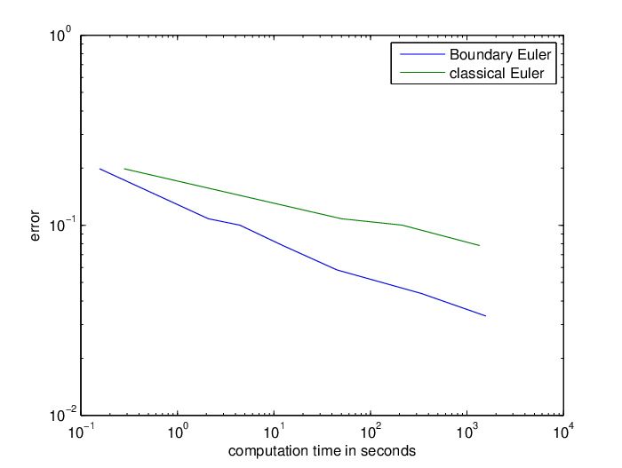
5.1 Speed of convergence
Refer to caption
Figure 1: Numerical errors of classical Euler scheme and boundary Euler scheme applied to (7) plotted against computational cost.
time Euler scheme [s] time boundary Euler [s] numerical error
0.821 0.156 0.1983
50.13 2.09 0.1083
213.73 4.43 0.1002
1350.25 12.355 0.0783
- 45.006 0.0583
- 336.79 0.0438
- 1570.93 0.0333
Table 1: Numerical errors of both schemes applied to (7) and corresponding computational cost.

For measuring the speed of convergence, we consider the ordinary differential inclusion

x′​(t)∈x⁡(t)+B1​(0)∞,x⁡(0)=0∈ℝ2,x^{\prime}(t)\in x(t)+B_{1}(0)_{\infty},\quad x(0)=0\in\mathbbm{R}^{2}, (7)

because the behavior of the numerical error is realistic while the inclusion is simple enough to admit the closed solution

ℛ⁡(T,{0})=Bet−1​(0)∞.\mathcal{R}(T,\{0\})=B_{e^{t}-1}(0)_{\infty}.

Moreover, the simple structure of the reachable set allows a reliable computation of the numerical errors w.r.t. the Hausdorff distance. The numerical errors and the corresponding computation times (on an ordinary laptop) are listed in Table 1 and visualized in Figure 1.

As explained in [4], it is reasonable to use the spatial discretization parameter ρ=h2\rho=h^{2}. It is doubtful whether the notion of an order of convergence makes sense in the set-valued context, because the performance of the schemes depends heavily on the space dimension. In this particular example, however, the estimated rates of convergence in terms of the computational costs necessary to achieve a given precision are 0.108 for the classical Euler scheme and 0.192 for the Boundary Euler, which makes a remarkable difference.

5.2 Topological changes of the reachable set

Refer to caption
Figure 2: The boundary Euler scheme applied to (8) and change of topology of the reachable set.
Refer to caption
Figure 3: A closeup of the critical time-step where the reachable set of the boundary Euler scheme applied to (8) changes its topology. The green rectangle in the first plot indicates the location of the magnified region. Points generating or being part of the outer layer are colored red, points generating or being part of the boundary of the reachable set are colored blue.

Unlike sets transported by ordinary differential equations, sets evolving under differential inclusions can change their topology. Consider the nonlinear ordinary differential inclusion

(x1′x2′)=(x1​(1−|x1|)−x1​x2x14−1/2)+B1/5​(0)∞,x⁡(0)=0∈ℝ2.\begin{pmatrix}x_{1}^{\prime}\\ x_{2}^{\prime}\end{pmatrix}=\begin{pmatrix}x_{1}(1-|x_{1}|)-x_{1}x_{2}\\ x_{1}^{4}-1/2\end{pmatrix}+B_{1/5}(0)_{\infty},\quad x(0)=0\in\mathbbm{R}^{2}. (8)

The reachable set ℛ⁡(T,{0})\mathcal{R}(T,\{0\}) of inclusion (8) is simply connected for T∈[0,5.275]T\in[0,5.275], but not for T=5.3T=5.3. The evolution of the reachable set for h=0.025h=0.025 and ρ=h2\rho=h^{2} is shown in Figure 2.

A closeup of the critical transition is depicted in Figure 3, which needs some explanation. The small green box in the first plot indicates the location of the magnified spot, and the second shows the situation at this location after 210 iterations. The blue line is the boundary ∂ρ0ℛ~h​(5.275,{0})\partial_{\rho}^{0}\tilde{\mathcal{R}}_{h}(5.275,\{0\}) of the reachable set, and the red line is the layer ∂ρ1ℛ~h​(5.275,{0})\partial_{\rho}^{1}\tilde{\mathcal{R}}_{h}(5.275,\{0\}) of exterior points the algorithm needs to keep track of the topology of the set.

Refer to caption
Figure 4: Failure of the boundary Euler scheme for disconnected initial sets.

The third plot shows the set S1S_{1} (specified in the algorithm) that contains the layer ∂ρ1ℛ~h​(5.3,{0})\partial_{\rho}^{1}\tilde{\mathcal{R}}_{h}(5.3,\{0\}) of exterior points of the set ℛ~h​(5.3,{0})\tilde{\mathcal{R}}_{h}(5.3,\{0\}) to be computed. In the fourth plot, the set S1S_{1} is overlaid by S00∪S0−1S_{0}^{0}\cup S_{0}^{-1}, deleting everything but ∂ρ1ℛ~h​(5.3,{0})\partial_{\rho}^{1}\tilde{\mathcal{R}}_{h}(5.3,\{0\}) from S1S_{1}, and in the fifth, only those points of S00∪S0−1S_{0}^{0}\cup S_{0}^{-1} are kept that have a neighbor in ∂ρ1ℛ~h​(5.3,{0})\partial_{\rho}^{1}\tilde{\mathcal{R}}_{h}(5.3,\{0\}), so that S00∪S0−1S_{0}^{0}\cup S_{0}^{-1} is reduced to ∂ρ0ℛ~h​(5.3,{0})\partial_{\rho}^{0}\tilde{\mathcal{R}}_{h}(5.3,\{0\}).

In the following plots, this procedure is repeated, but the seventh plot shows that in this step S00∪S0−1S_{0}^{0}\cup S_{0}^{-1} erases a large portion of S1S_{1}, so that no new boundary is generated in that place and the change of topology of the exact reachable set is reproduced by the discrete approximation.

The opposite effect – the closing of a hole in the reachable set – can be observed in the simple example

x′​(t)∈B1​(0)∞,x⁡(0)∈X0={x∈ℝ2:1≤|x|∞≤2}x^{\prime}(t)\in B_{1}(0)_{\infty},\quad x(0)\in X_{0}=\{x\in\mathbbm{R}^{2}:1\leq|x|_{\infty}\leq 2\} (9)

that is not displayed here, because the mechanism behind the change of topology is essentially the same as for inclusion (8).

Refer to caption
Figure 5: Failure of the boundary Euler scheme because of L​h≥1/4Lh\geq 1/4.

5.3 Failure due to violated assumptions

The proof of the propriety of the boundary Euler scheme relies on the assumption that the initial set Bα∗​(X0)∩ΔρB_{\alpha^{*}}(X_{0})\cap\Delta_{\rho} is chain-connected. Applying one step of the boundary Euler to the simple differential inclusion (9) with disconnected initial set X0={(0,1),(1,0)}X_{0}=\{(0,1),(1,0)\}, h=1/4h=1/4, and ρ=1/16\rho=1/16 demonstrates that this assumption is not imposed for convenience, but relevant for practical computation. Figure 4 shows that the boundary ∂ρ0ℛ~​(1/4,X0)\partial_{\rho}^{0}\tilde{\mathcal{R}}(1/4,X_{0}) of the reachable set at time 1/41/4 is not correctly computed, because inner points of the reachable set are marked as boundary points. Therefore, if the initial set is disconnected, the preliminary version of the boundary Euler scheme must be used, which outperforms the classical Euler scheme, but is slower than the boundary Euler scheme in its final form.

Figure 5 shows what may happen if the assumption L​h<1/4Lh<1/4 is violated. In example (8), the boundaries of the discrete reachable sets do not only become more and more inaccurate, but literally fall apart when hh is increased. This effect is known for the classical Euler scheme, but it is only ungainly and not harmful there, because the discrete reachable sets still approximate the original reachable sets with prescribed accuracy. Since the boundary Euler is supposed to compute a real boundary, the effect is not tolerable in this setting.

References

  • [1] J. P. Aubin and A. Cellina. Differential Inclusions, volume 264 of Grundlehren der mathematischen Wissenschaften. Springer, Berlin, 1984.
  • [2] J.-P. Aubin and H. Frankowska. Set-Valued Analysis. Birkhäuser, Boston, 1990.
  • [3] R. Baier, M. Gerdts, and I. Xausa. Approximation of reachable sets using optimal control algorithms. To appear in Numerical Algebra, Control and Optimization.
  • [4] W.-J. Beyn and J. Rieger. Numerical fixed grid methods for differential inclusions. Computing, 81(1):91–106, 2007.
  • [5] W.-J. Beyn and J. Rieger. The implicit Euler scheme for one-sided Lipschitz differential inclusions. DCDS-B, 14:409–428, 2010.
  • [6] K. Deimling. Multivalued Differential Equations. De Gruyter, Berlin, 1992.
  • [7] A. Dontchev and E. Farkhi. Error estimates for discretized differential inclusions. Computing, 41:349–358, 1989.
  • [8] H.G. Eggleston. Convexity, volume 47 of Cambridge Tracts in Mathematics. Cambridge University Press.
  • [9] F. Lempio and V. Veliov. Discrete approximations of differential inclusions. Bayreuther Mathematische Schriften, 54:149–232, 1998.
  • [10] M. D. P. Monteiro Marques. Sur la frontière d’un convexe mobile. Atti Accad. Naz. Lincei Rend. Cl. Sci. Fis. Mat. Natur. Ser. VIII, 77:71–75, 1984.
  • [11] J. Rieger. Discretizations of linear elliptic partial differential inclusions. Numerical Functional Analysis and Optimization, 32(8):904–925, 2011.
  • [12] M. Sandberg. Convergence of the forward Euler method for nonconvex differential inclusions. SIAM J. Numer. Anal., 47(1):308–320, 2008.
  • [13] V. Veliov. Second order discrete approximations to strongly convex differential inclusions. Systems and Control Letters, 13:263–269, 1989.
  • [14] E. Zeidler. Nonlinear Functional Analysis and its Applications, volume 1. Springer, Heidelberg, 1985.