跳到论文正文
W Papers独立论文阅读器 arXiv:1308.3639 论文正文 计算阅读时间 · 0%
引用这篇论文根据当前论文元数据生成,正式投稿前建议核对。


License: arXiv.org perpetual non-exclusive license
arXiv:1308.3639v1 [math.OC] 16 Aug 2013

A numerical method for the solution of relaxed one-sided Lipschitz algebraic inclusions

Wolf-Jürgen Beyn Note: Supported by CRC 701 ’Spectral Structures and Topological Methods in Mathematics’, Bielefeld University. Affiliation: Fakultät für Mathematik, Universität Bielefeld Affiliation: Postfach 100131, D-33501 Bielefeld, Germany Affiliation: Janosch Rieger Affiliation: Institut für Mathematik, Universität Frankfurt Affiliation: Postfach 111932, D-60054 Frankfurt a.M., Germany
August 24, 2026
Abstract

An existing solvability result for relaxed one-sided Lipschitz algebraic inclusions is substantially improved. This enhanced solvability result allows the design of a very robust numerical method for the approximation of a solution of the algebraic inclusion. Sharp error estimates for this method, illustrative analytic examples and a numerical example are provided.

1 Introduction and notation

The solution of nonlinear equations and inclusions is one of the fundamental problems in pure and applied mathematics. A multitude of analytical concepts for the identification and localization of solutions as well as numerical methods for their approximation have been developed that exploit characteristic features of particular types of mappings. In this paper, solutions of the algebraic inclusion

y¯∈F⁡(x)\bar{y}\in F(x) (1)

with given y¯∈ℝd\bar{y}\in\mathbbm{R}^{d} are considered for the class of relaxed one-sided Lipschitz (ROSL, see below) multivalued mappings FF with negative one-sided Lipschitz constant. The relatively modern ROSL property was introduced and investigated in [5] and other works of the same author. It generalizes the classical one-sided Lipschitz property and is a key criterion for the analysis of differential inclusions and numerical approximations of their solution sets (see e.g. [6]), so that algebraic inclusions of type (1) with ROSL multifunction FF arise in a natural way. Moreover, the ROSL property is intimately related to the notion of metric regularity, which is discussed in [7, Chapter 3].

A solvability result for the class of multivalued mappings satisfying the ROSL property was proved in [3, Corollary 3]. It states that given an initial guess xx, there exists a solution x¯\bar{x} of (1) in a closed ball centered at xx with radius depending on the defect dist⁡(y¯,F⁡(x))\dist(\bar{y},F(x)). A substantially improved version of this result is given in Theorem 1 below, which allows to localize a solution of (1) in a smaller ball BB with x∈∂Bx\in\partial B and thus specifies not only a distance but also a direction in which a solution is to be found (see Figure 1). If the mapping FF is in addition Lipschitz continuous, then the localization of the solution can once again be improved.

This information can be used to design a very robust numerical algorithm for the approximation of a solution of (1) that uses the current state as initial guess for the improved solvability theorem and defines the next iterate as the center of the ball BB. Proposition 5 provides error estimates for this numerical scheme, and Example 7 shows that they are sharp for dimension d>1d>1. The one-dimensional case is treated separately in Proposition 9. Enhancements of the numerical method for LL-Lipschitz multimaps FF are briefly analyzed in Propositions 10 and 11, and a numerical example is provided.

Let ℝd\mathbbm{R}^{d} be equipped with the Euclidean norm |⋅||\cdot| and the Euclidean inner product ⟨⋅,⋅⟩\langle\cdot,\cdot\rangle. A closed ball with radius R≥0R\geq 0 centered at x∈ℝdx\in\mathbbm{R}^{d} will be denoted by BR​(x)=B​(x,R)B_{R}(x)=B(x,R). The family of nonempty compact and convex subsets of ℝd\mathbbm{R}^{d} is denoted by 𝒞​𝒞​(ℝd)\mathcal{CC}(\mathbbm{R}^{d}), the one-sided and the symmetric Hausdorff-distances of two sets A,B∈𝒞​𝒞​(ℝd)A,B\in\mathcal{CC}(\mathbbm{R}^{d}) are defined by

dist⁡(A,B)\displaystyle\dist(A,B) :=supa∈Ainfb∈B|a−b|,\displaystyle:=\sup_{a\in A}\inf_{b\in B}|a-b|,
distH⁡(A,B)\displaystyle\dist_{H}(A,B) :=max⁡{dist⁡(A,B),dist⁡(B,A)},\displaystyle:=\max\{\dist(A,B),\dist(B,A)\},

and the so-called norm of a set A∈𝒞​𝒞​(ℝd)A\in\mathcal{CC}(\mathbbm{R}^{d}) is ‖A‖:=maxa∈A⁡|a|\|A\|:=\max_{a\in A}|a|. The metric projection of a point y∈ℝdy\in\mathbbm{R}^{d} to a set A∈𝒞​𝒞​(ℝd)A\in\mathcal{CC}(\mathbbm{R}^{d}) is the unique point Proj⁡(y,A)∈A\Proj(y,A)\in A satisfying |y−Proj⁡(y,A)|=dist⁡(y,A)|y-\Proj(y,A)|=\dist(y,A).

Consider a multivalued mapping F:ℝd→𝒞​𝒞​(ℝd)F:\mathbbm{R}^{d}\rightarrow\mathcal{CC}(\mathbbm{R}^{d}). It is called upper semicontinuous (usc) at x∈ℝdx\in\mathbbm{R}^{d} if

dist⁡(F⁡(x′),F⁡(x))→0​as​x′→x,\dist(F(x^{\prime}),F(x))\rightarrow 0\ \text{as}\ x^{\prime}\rightarrow x,

usc if it is usc at every x∈ℝdx\in\mathbbm{R}^{d}, and LL-Lipschitz with L≥0L\geq 0 if

distH⁡(F⁡(x),F⁡(x′))≤L|x−x′|for all​x,x′∈ℝd.\dist_{H}(F(x),F(x^{\prime}))\leq L|x-x^{\prime}|\ \text{for all}\ x,x^{\prime}\in\mathbbm{R}^{d}.

The mapping is called relaxed one-sided Lipschitz with constant l∈ℝl\in\mathbbm{R} (ll-ROSL) if for any x,x′∈ℝdx,x^{\prime}\in\mathbbm{R}^{d} and y∈F⁡(x)y\in F(x), there exists some y′∈F⁡(x′)y^{\prime}\in F(x^{\prime}) such that

⟨y−y′,x−x′⟩≤l​|x−x′|2.\langle y-y^{\prime},x-x^{\prime}\rangle\leq l|x-x^{\prime}|^{2}.

2 Solvability of ROSL algebraic inclusions

The following theorem is the core of this paper. It is a strongly improved version of the solvability theorem given in [3, Corollary 3], and its assumptions on the mapping FF can still be weakened (see Remark 3). Its statement is illustrated in Figure 1.

Theorem 1.

Let F:ℝd→𝒞​𝒞​(ℝd)F:\mathbbm{R}^{d}\rightarrow\mathcal{CC}(\mathbbm{R}^{d}) be usc and ROSL with constant l<0l<0, and let x~∈ℝd\tilde{x}\in\mathbbm{R}^{d} and y¯∈ℝd\bar{y}\in\mathbbm{R}^{d} be given. Then there exists a solution

x¯∈SF​(y¯):={x∈ℝd:y¯∈F⁡(x)}\bar{x}\in S_{F}(\bar{y}):=\{x\in\mathbbm{R}^{d}:\bar{y}\in F(x)\}

satisfying

|x¯−(x~+12​l​(y¯−Proj⁡(y¯,F⁡(x~))))|≤−12​l​dist⁡(y¯,F⁡(x~)),|\bar{x}-(\tilde{x}+\frac{1}{2l}(\bar{y}-\Proj(\bar{y},F(\tilde{x}))))|\leq-\frac{1}{2l}\dist(\bar{y},F(\tilde{x})), (2)

and the set SF​(y¯)S_{F}(\bar{y}) is closed. If FF is in addition LL-Lipschitz, then for any x¯∈SF​(y¯)\bar{x}\in S_{F}(\bar{y}),

|x¯−x~|≥1L​dist⁡(y¯,F⁡(x~)).|\bar{x}-\tilde{x}|\geq\frac{1}{L}\dist(\bar{y},F(\tilde{x})). (3)
Refer to caption
Figure 1: Schematic illustration of Theorem 1. The solvability theorem given in [3, Corollary 3] only guarantees the existence of a solution x¯\bar{x} of y¯∈F⁡(x)\bar{y}\in F(x) in the (blue) ball of radius −1l​dist⁡(y¯,F⁡(x~))-\frac{1}{l}\dist(\bar{y},F(\tilde{x})) centered at x~\tilde{x}. Theorem 1 guarantees such a solution in the (red) ball with radius −12​l​dist⁡(y¯,F⁡(x~))-\frac{1}{2l}\dist(\bar{y},F(\tilde{x})) centered at x~c=x+12​l​(y¯−Proj⁡(y¯,F⁡(x~)))\tilde{x}_{c}=x+\frac{1}{2l}(\bar{y}-\Proj(\bar{y},F(\tilde{x}))), and if FF is LL-Lipschitz, it states that no solution is contained in the (black) ball of radius 1L​dist⁡(y¯,F⁡(x~))\frac{1}{L}\dist(\bar{y},F(\tilde{x})) centered at x~\tilde{x}.
Lemma 2.

Let F:ℝd→𝒞​𝒞​(ℝd)F:\mathbbm{R}^{d}\rightarrow\mathcal{CC}(\mathbbm{R}^{d}) be usc and ROSL with constant l<0l<0. Then the inclusion 0∈F⁡(x)0\in F(x) has a solution x¯\bar{x} with

|x¯|≤−1l​dist⁡(0,F⁡(0))|\bar{x}|\leq-\frac{1}{l}\dist(0,F(0)) (4)

that satisfies the property

⟨−Proj⁡(0,F⁡(0)),x¯⟩≤l​|x¯|2.\langle-\Proj(0,F(0)),\bar{x}\rangle\leq l|\bar{x}|^{2}. (5)
Proof.

Let y0:=Proj⁡(0,F⁡(0))y_{0}:=\Proj(0,F(0)) be the element with minimal norm. By the ROSL property of FF, the mapping Ψ:ℝd→𝒞​𝒞​(ℝd)\Psi:\mathbbm{R}^{d}\rightarrow\mathcal{CC}(\mathbbm{R}^{d}) given by

Ψ⁡(x):=F⁡(x)∩{y∈ℝd:⟨y−y0,x⟩≤l​|x|2}\Psi(x):=F(x)\cap\{y\in\mathbbm{R}^{d}:\langle y-y_{0},x\rangle\leq l|x|^{2}\}

has nonempty images. By [1, Theorem 1.1.1], it is usc. Define the usc mapping G:ℝd→𝒞​𝒞​(ℝd)G:\mathbbm{R}^{d}\rightarrow\mathcal{CC}(\mathbbm{R}^{d}) by

G⁡(x):=x+α​Ψ​(x)G(x):=x+\alpha\Psi(x)

with some α>0\alpha>0. Take y∈Ψ⁡(x)y\in\Psi(x) and set z:=x+α​yz:=x+\alpha y. Then

|z|2\displaystyle|z|^{2} =\displaystyle= |x|2+2​α​⟨y,x⟩+α2​|y|2\displaystyle|x|^{2}+2\alpha\langle y,x\rangle+\alpha^{2}|y|^{2}
=\displaystyle= |x|2+2​α​⟨y−y0,x⟩+2​α​⟨y0,x⟩+α2​|y|2\displaystyle|x|^{2}+2\alpha\langle y-y_{0},x\rangle+2\alpha\langle y_{0},x\rangle+\alpha^{2}|y|^{2}
≤\displaystyle\leq |x|2+2​α​l​|x|2+2​α​|x|​dist⁡(0,F⁡(0))+α2​|y|2.\displaystyle|x|^{2}+2\alpha l|x|^{2}+2\alpha|x|\dist(0,F(0))+\alpha^{2}|y|^{2}.

Thus, if R>−1l​dist⁡(0,F⁡(0))R>-\frac{1}{l}\dist(0,F(0)), |x|≤R|x|\leq R, and α\alpha is so small that 1+2​α​l≥01+2\alpha l\geq 0, then

|z|2\displaystyle|z|^{2} ≤\displaystyle\leq R2+2​α​(l​R+dist⁡(0,F⁡(0)))​R+α2​|y|2\displaystyle R^{2}+2\alpha(lR+\dist(0,F(0)))R+\alpha^{2}|y|^{2} (6)
<\displaystyle< R2+α2​|y|2.\displaystyle R^{2}+\alpha^{2}|y|^{2}.

As FF is usc,

MR:=supx∈BR​(0)‖F⁡(x)‖<∞,M_{R}:=\sup_{x\in B_{R}(0)}\|F(x)\|<\infty,

and there exists an α>0\alpha>0 such that |z|2≤R2|z|^{2}\leq R^{2} follows from (6). This means that for this fixed α\alpha,

H⁡(x):=G⁡(x)∩BR​(0)≠∅​ for all ​x∈BR​(0),H(x):=G(x)\cap B_{R}(0)\neq\emptyset\text{ for all }x\in B_{R}(0),

and H⁡(⋅)H(\cdot) is also usc. By the Kakutani Theorem (see [2, Theorem 3.2.3]), HH and thus also GG have a fixed point xRx_{R} in BR​(0)B_{R}(0), which implies that 0∈Ψ⁡(xR)0\in\Psi(x_{R}).

In particular, we find elements xn∈B⁡(0,−1l​dist⁡(0,F⁡(0))+1/n)x_{n}\in B(0,-\frac{1}{l}\dist(0,F(0))+1/n) for all n∈ℕn\in\mathbbm{N} such that 0∈Ψ⁡(xn)0\in\Psi(x_{n}). As B⁡(0,−1l​dist⁡(0,F⁡(0))+1)B(0,-\frac{1}{l}\dist(0,F(0))+1) is compact, there exists a convergent subsequence of {xn}n∈ℕ\{x_{n}\}_{n\in\mathbbm{N}} with limit

x¯∈B⁡(0,−1l​dist⁡(0,F⁡(0))).\bar{x}\in B(0,-\frac{1}{l}\dist(0,F(0))).

Since Ψ\Psi is usc,

0∈Ψ⁡(x¯)⊂F⁡(x¯).0\in\Psi(\bar{x})\subset F(\bar{x}).

Property (5) follows from the construction of Ψ\Psi. ∎

Proof of Theorem 1.

Consider the set-valued mapping

G⁡(z):=F⁡(z+x~)−y¯,G(z):=F(z+\tilde{x})-\bar{y},

which is ROSL with constant ll. By the above theorem, there exists some

z¯∈B⁡(0,−1l​dist⁡(0,G⁡(0)))=B⁡(0,−1l​dist⁡(y¯,F⁡(x~)))\bar{z}\in B(0,-\frac{1}{l}\dist(0,G(0)))=B(0,-\frac{1}{l}\dist(\bar{y},F(\tilde{x})))

such that 0∈G⁡(z¯)0\in G(\bar{z}) or y¯∈F⁡(x¯)\bar{y}\in F(\bar{x}), where x¯=x~+z¯\bar{x}=\tilde{x}+\bar{z}. Property (5),

⟨−Proj⁡(0,G⁡(0)),z¯⟩=⟨−Proj⁡(0,F⁡(x~)−y¯),x¯−x~⟩=⟨y¯−Proj⁡(y¯,F⁡(x~)),x¯−x~⟩,\langle-\Proj(0,G(0)),\bar{z}\rangle=\langle-\Proj(0,F(\tilde{x})-\bar{y}),\bar{x}-\tilde{x}\rangle=\langle\bar{y}-\Proj(\bar{y},F(\tilde{x})),\bar{x}-\tilde{x}\rangle,

and

l​|z¯|2=l​|x¯−x~|2.l|\bar{z}|^{2}=l|\bar{x}-\tilde{x}|^{2}.

imply that

⟨y¯−Proj⁡(y¯,F⁡(x~)),x¯−x~⟩≤l​|x¯−x~|2,\langle\bar{y}-\Proj(\bar{y},F(\tilde{x})),\bar{x}-\tilde{x}\rangle\leq l|\bar{x}-\tilde{x}|^{2},

which is equivalent with (2).

The fact that SF​(y¯)S_{F}(\bar{y}) is closed follows directly from the usc property of FF.

If FF is in addition LL-Lipschitz and x¯∈SF​(y¯)\bar{x}\in S_{F}(\bar{y}), then

dist⁡(y¯,F⁡(x~))≤dist⁡(F⁡(x¯),F⁡(x~))≤L​|x¯−x~|\dist(\bar{y},F(\tilde{x}))\leq\dist(F(\bar{x}),F(\tilde{x}))\leq L|\bar{x}-\tilde{x}|

implies

|x¯−x~|≥1L​dist⁡(y¯,F⁡(x~)).|\bar{x}-\tilde{x}|\geq\frac{1}{L}\dist(\bar{y},F(\tilde{x})).

∎

Remark 3.

The assumptions of Theorem 1 can be weakened. In particular, the set-valued mapping FF may be defined only on B:=B⁡(x~,−1l​dist⁡(y¯,F⁡(x~)))B:=B(\tilde{x},-\frac{1}{l}\dist(\bar{y},F(\tilde{x}))).

  • a)

    In order to obtain the existence of a solution and estimate (2), it is sufficient to require that F:B→𝒞​𝒞​(ℝd)F:B\rightarrow\mathcal{CC}(\mathbbm{R}^{d}) is usc and that

    ∀x∈B​∃y∈F⁡(x):⟨y−Proj⁡(y¯,F⁡(x~)),x−x~⟩≤l​|x−x~|2.\forall\,x\in B\ \exists\,y\in F(x):\ \langle y-\Proj(\bar{y},F(\tilde{x})),x-\tilde{x}\rangle\leq l|x-\tilde{x}|^{2}. (7)

    The mapping FF can then be extended as in [4, proof of Theorem 2] to a set-valued function F~:ℝd→𝒞​𝒞​(ℝd)\tilde{F}:\mathbbm{R}^{d}\rightarrow\mathcal{CC}(\mathbbm{R}^{d}) that coincides with FF on BB, is usc, and satisfies property (7) for all x∈ℝdx\in\mathbbm{R}^{d}. The proof of Theorem 1 can be applied to the mapping F~\tilde{F} without changes.

  • b)

    To show estimate (3), it is enough for F:B→𝒞​𝒞​(ℝd)F:B\rightarrow\mathcal{CC}(\mathbbm{R}^{d}) to be LL-Lipschitz relative to x~\tilde{x} in the sense that

    distH⁡(F⁡(x),F⁡(x~))≤L|x−x~|for all​x∈B.\dist_{H}(F(x),F(\tilde{x}))\leq L|x-\tilde{x}|\ \text{for all}\ x\in B.

    It follows directly that for any x¯∈SF​(y¯)∩B\bar{x}\in S_{F}(\bar{y})\cap B (and hence for all x¯∈SF​(y¯)\bar{x}\in S_{F}(\bar{y})),

    |x¯−x~|≥1L​dist⁡(y¯,F⁡(x~)).|\bar{x}-\tilde{x}|\geq\frac{1}{L}\dist(\bar{y},F(\tilde{x})).
Remark 4.

It is unclear if additional assumptions are needed to guarantee the connectedness of SF​(y¯)S_{F}(\bar{y}). This question is linked with the parametrization problem for ROSL multifunctions (see Lemma 12 in [3]).

3 A numerical solver for ROSL algebraic inclusions

Throughout this section, the mapping F:ℝd→𝒞​𝒞​(ℝd)F:\mathbbm{R}^{d}\rightarrow\mathcal{CC}(\mathbbm{R}^{d}) will be assumed to be ll-ROSL and LL-Lipschitz. A numerical method for finding a solution x¯\bar{x} of the inclusion y¯∈F⁡(x)\bar{y}\in F(x) can be deduced directly from Theorem 1 by defining the next iterate of the scheme as the center of the ball specified by (2).

Proposition 5.

Let L<−2​lL<-2l, and let x0∈ℝdx_{0}\in\mathbbm{R}^{d} and y¯∈ℝd\bar{y}\in\mathbbm{R}^{d} be given. Then the sequence {xn}n∈ℕ\{x_{n}\}_{n\in\mathbbm{N}} defined by

xn+1:=Φ⁡(xn):=xn+12​l​(y¯−Proj⁡(y¯,F⁡(xn)))x_{n+1}:=\Phi(x_{n}):=x_{n}+\frac{1}{2l}(\bar{y}-\Proj(\bar{y},F(x_{n}))) (8)

converges to a solution x¯\bar{x} of the inclusion y¯∈F⁡(x)\bar{y}\in F(x) and satisfies the estimates

dist⁡(xn,SF​(y¯))≤Ln−1|2​l|n​dist⁡(y¯,F⁡(x0))\dist(x_{n},S_{F}(\bar{y}))\leq\frac{L^{n-1}}{|2l|^{n}}\dist(\bar{y},F(x_{0})) (9)

and

|xn−x¯|≤−12​l​Ln|2​l|n1−L|2​l|​dist⁡(y¯,F⁡(x0))|x_{n}-\bar{x}|\leq-\frac{1}{2l}\frac{\frac{L^{n}}{|2l|^{n}}}{1-\frac{L}{|2l|}}\dist(\bar{y},F(x_{0})) (10)

for n≥1n\geq 1.

Proof.

Set vn:=y¯−Proj⁡(y¯,F⁡(xn))v_{n}:=\bar{y}-\Proj(\bar{y},F(x_{n})) for n∈ℕn\in\mathbbm{N}. Then (2) implies that there exists some x¯n∈SF​(y¯)\bar{x}_{n}\in S_{F}(\bar{y}) such that

dist⁡(xn+1,SF​(y¯))≤|x¯n−(xn+12​l​vn)|≤−12​l​|vn|.\displaystyle\dist(x_{n+1},S_{F}(\bar{y}))\leq|\bar{x}_{n}-(x_{n}+\frac{1}{2l}v_{n})|\leq-\frac{1}{2l}|v_{n}|. (11)

Now

|vn+1|\displaystyle|v_{n+1}| =dist⁡(y¯,F⁡(xn+1))≤dist⁡(y¯,F⁡(x¯n))+dist⁡(F⁡(x¯n),F⁡(xn+12​l​vn))\displaystyle=\dist(\bar{y},F(x_{n+1}))\leq\dist(\bar{y},F(\bar{x}_{n}))+\dist(F(\bar{x}_{n}),F(x_{n}+\frac{1}{2l}v_{n}))
≤L​|x¯n−(xn+12​l​vn)|≤−L2​l​|vn|\displaystyle\leq L|\bar{x}_{n}-(x_{n}+\frac{1}{2l}v_{n})|\leq-\frac{L}{2l}|v_{n}|

by (11) for n∈ℕn\in\mathbbm{N}, so that

|vn|≤Ln|2​l|n​|v0|,|v_{n}|\leq\frac{L^{n}}{|2l|^{n}}|v_{0}|,

and again by (11), we have

dist⁡(xn,SF​(y))≤−12​l​|vn−1|≤Ln−1|2​l|n​|v0|\dist(x_{n},S_{F}(y))\leq-\frac{1}{2l}|v_{n-1}|\leq\frac{L^{n-1}}{|2l|^{n}}|v_{0}| (12)

for n≥1n\geq 1, which shows (9). Since

|xn+1−xn|≤−12​l​|vn|≤−12​l​Ln|2​l|n​|v0||x_{n+1}-x_{n}|\leq-\frac{1}{2l}|v_{n}|\leq-\frac{1}{2l}\frac{L^{n}}{|2l|^{n}}|v_{0}| (13)

for all n∈ℕn\in\mathbbm{N}, the sequence {xn}n∈ℕ\{x_{n}\}_{n\in\mathbbm{N}} is Cauchy and converges to some x¯∈ℝd\bar{x}\in\mathbbm{R}^{d}. As SF​(y¯)S_{F}(\bar{y}) is closed, estimate (12) shows that x¯∈SF​(y¯)\bar{x}\in S_{F}(\bar{y}). Finally, for all n,N∈ℕn,N\in\mathbbm{N} with N>nN>n, it follows from (13) that

|xN−xn|\displaystyle|x_{N}-x_{n}| ≤∑j=nN−1|xj+1−xj|≤−12​l|v0|∑j=nN−1Lj|2​l|j\displaystyle\leq\sum_{j=n}^{N-1}|x_{j+1}-x_{j}|\leq-\frac{1}{2l}|v_{0}|\sum_{j=n}^{N-1}\frac{L^{j}}{|2l|^{j}}
=−12​l|v0|Ln|2​l|n​∑j=0N−n−1Lj|2​l|j=−12​l​|v0|​Ln|2​l|n​1−LN−n|2​l|N−n1−L|2​l|\displaystyle=-\frac{1}{2l}|v_{0}|\frac{L^{n}}{|2l|^{n}}\sum_{j=0}^{N-n-1}\frac{L^{j}}{|2l|^{j}}=-\frac{1}{2l}|v_{0}|\frac{L^{n}}{|2l|^{n}}\frac{1-\frac{L^{N-n}}{|2l|^{N-n}}}{1-\frac{L}{|2l|}}
≤−12​l​|v0|​Ln|2​l|n1−L|2​l|.\displaystyle\leq-\frac{1}{2l}|v_{0}|\frac{\frac{L^{n}}{|2l|^{n}}}{1-\frac{L}{|2l|}}.

Passing to the limit as N→∞N\rightarrow\infty yields (10). ∎

Remark 6.

By Theorem 1, any numerical iteration {xn}n∈ℕ\{x_{n}\}_{n\in\mathbbm{N}} will converge to SF​(y)S_{F}(y) provided that the sequence of defects vnv_{n} converges to zero. A simple modification of the proof of Proposition 5 shows that the defect at any point in the interval xn+(1l,0)​vnx_{n}+(\frac{1}{l},0)v_{n} is smaller than at xnx_{n} and that for r∈[0,−12​l)r\in[0,-\frac{1}{2l}) and |xn+1−(xn+12​l​vn)|≤r|x_{n+1}-(x_{n}+\frac{1}{2l}v_{n})|\leq r for all n∈ℕn\in\mathbbm{N}, the algorithm still converges linearly with reduced speed. This means that even if ll is unknown, it is possible to find a next iterate with smaller defect according to simple trust region strategies.

The following example shows that Proposition 5 is sharp (apart from statement (10)).

Example 7.

Let l<0l<0 and L≥−lL\geq-l, and set F⁡(x):=l​x+α​x⟂F(x):=lx+\alpha x^{\perp}, where α:=L2−l2\alpha:=\sqrt{L^{2}-l^{2}} and x⟂:=(x(2),−x(1))x^{\perp}:=(x^{(2)},-x^{(1)}) is the image of xx under the rotation with angle −π/2-\pi/2 around the origin. The single-valued mapping FF is ll-OSL and LL-Lipschitz. If the numerical method (8) is applied to the problem 0=F⁡(x)0=F(x), we have

Φ⁡(x)=x−12​l​F​(x)=12​(1−α/lα/l1)​x.\Phi(x)=x-\frac{1}{2l}F(x)=\frac{1}{2}\begin{pmatrix}1&-\alpha/l\\ \alpha/l&1\end{pmatrix}x.

The eigenvalues of the above matrix are λ1/2=12±α2​l​i\lambda_{1/2}=\frac{1}{2}\pm\frac{\alpha}{2l}i, i.e. the iteration converges if and only if L<−2​lL<-2l. Moreover,

‖12​(1−α/lα/l1)‖2=−L2​l,\|\frac{1}{2}\begin{pmatrix}1&-\alpha/l\\ \alpha/l&1\end{pmatrix}\|_{2}=-\frac{L}{2l},

so that the iteration converges with rate −L2​l-\frac{L}{2l} whenever L<−2​lL<-2l. In fact, it can be shown easily by using rotational symmetry of FF that estimate (9) is sharp for every initial state x0∈ℝ2x_{0}\in\mathbbm{R}^{2}.

The following example shows that the condition L<−2​lL<-2l is not sharp for convergence of the method (8) in d=1d=1.

Example 8.

Consider the function F:ℝ→ℝF:\mathbbm{R}\rightarrow\mathbbm{R} given by

F⁡(x)={−L+l⁡(x−1),1≤x−L​x,−1≤x≤1+L+l⁡(x+1),x≤−1F(x)=\left\{\begin{array}[]{ll}-L+l(x-1),&1\leq x\\ -Lx,&-1\leq x\leq 1\\ +L+l(x+1),&x\leq-1\end{array}\right.

with l<0l<0 and L≥−lL\geq-l. Clearly, FF is ll-OSL and LL-Lipschitz. Let xn∈[−1,1]x_{n}\in[-1,1] be a state of the root finding method that is supposed to solve 0=F⁡(x)0=F(x). Then

xn+1=xn−F⁡(xn)2​l=xn+L​xn2​l=(1+L2​l)​xn,x_{n+1}=x_{n}-\frac{F(x_{n})}{2l}=x_{n}+\frac{Lx_{n}}{2l}=(1+\frac{L}{2l})x_{n},

so that |xn+1|<|xn||x_{n+1}|<|x_{n}| if and only if L<−4​lL<-4l. Figure 2 illustrates the global behavior of the function FF and the numerical method Φ\Phi for characteristic ratios −L/l-L/l.

Refer to caption
Refer to caption
Figure 2: Behavior of the function FF from Example 8 and the corresponding numerical method Φ\Phi for l=−1l=-1 and characteristic values of LL. The red lines limit the central interval [−1,1][-1,1] in space and image. The value L=−4​lL=-4l is the critical threshold.

The gap between the condition L<−2​lL<-2l required for convergence in Proposition 5 and the condition L<−4​lL<-4l observed in Example 8 is due to the fact that for multifunctions F:ℝ→𝒞​𝒞​(ℝ)F:\mathbbm{R}\rightarrow\mathcal{CC}(\mathbbm{R}), the ROSL property is much stronger than in ℝd\mathbbm{R}^{d} with d>1d>1. In this particular context, it is possible to derive estimates for some of the defects (see Case 1a in the following proof) that only depend on the one-sided Lipschitz constant ll and not on the Lipschitz constant LL.

Proposition 9.

Let F:ℝ→𝒞​𝒞​(ℝ)F:\mathbbm{R}\rightarrow\mathcal{CC}(\mathbbm{R}) be ll-ROSL and LL-Lipschitz with l<0l<0 and L<−4​lL<-4l, and let x0∈ℝx_{0}\in\mathbbm{R} and y¯∈ℝ\bar{y}\in\mathbbm{R} be given. Then the sequence {xn}n∈ℕ\{x_{n}\}_{n\in\mathbbm{N}} defined by

xn+1:=xn+12​l​(y¯−Proj⁡(y¯,F⁡(xn)))x_{n+1}:=x_{n}+\frac{1}{2l}(\bar{y}-\Proj(\bar{y},F(x_{n})))

converges to a solution x¯\bar{x} of the inclusion y¯∈F⁡(x)\bar{y}\in F(x) and satisfies the estimates

dist⁡(xn,SF​(y¯))≤−12​l​κn−1​dist⁡(y¯,F⁡(x0))\dist(x_{n},S_{F}(\bar{y}))\leq-\frac{1}{2l}\kappa^{n-1}\dist(\bar{y},F(x_{0})) (14)

and

|xn−x¯|≤−12​l​κn1−κ​dist⁡(y¯,F⁡(x0))|x_{n}-\bar{x}|\leq-\frac{1}{2l}\frac{\kappa^{n}}{1-\kappa}\dist(\bar{y},F(x_{0})) (15)

for n≥1n\geq 1, where κ:=max⁡{12,|1+L2​l|}\kappa:=\max\{\frac{1}{2},|1+\frac{L}{2l}|\}.

Proof.

Let −2​l≤L<−4​l-2l\leq L<-4l and set vn:=y¯−Proj⁡(y¯,F⁡(xn))v_{n}:=\bar{y}-\Proj(\bar{y},F(x_{n})) for n∈ℕn\in\mathbbm{N}. Without loss of generality, y¯∉F⁡(xn)\bar{y}\notin F(x_{n}) and y¯∉F⁡(xn+1)\bar{y}\notin F(x_{n+1}), because otherwise the sequences {vn}\{v_{n}\} and {xn}\{x_{n}\} become constant and all estimates are trivially satisfied. As F⁡(xn)F(x_{n}) is an interval, there are only two cases.

Case 1: y¯>y\bar{y}>y for all y∈F⁡(xn)y\in F(x_{n}).
In particular, vn>0v_{n}>0. If x¯∈SF​(y¯)\bar{x}\in S_{F}(\bar{y}), then the ROSL property yields some y∈F⁡(xn)y\in F(x_{n}) such that

(y¯−y)​(x¯−xn)≤l​|x¯−xn|2,(\bar{y}-y)(\bar{x}-x_{n})\leq l|\bar{x}-x_{n}|^{2},

which implies x¯≤xn\bar{x}\leq x_{n}. By Theorem 1,

Sn:=SF​(y¯)∩[xn+1l​vn,xn−1L​vn]≠∅.S_{n}:=S_{F}(\bar{y})\cap[x_{n}+\frac{1}{l}v_{n},x_{n}-\frac{1}{L}v_{n}]\neq\emptyset.

Let x¯n:=max⁡Sn\bar{x}_{n}:=\max S_{n}. Without loss of generality, xn≠x¯n≠xn+1x_{n}\neq\bar{x}_{n}\neq x_{n+1}, because otherwise the sequences {vn}\{v_{n}\} and {xn}\{x_{n}\} become constant. There are two subcases.

Subcase 1a: x¯n∈[xn+1lvn,xn+12​lvn)\bar{x}_{n}\in[x_{n}+\frac{1}{l}v_{n},x_{n}+\frac{1}{2l}v_{n}).
Assume that there exists some y∗∈F⁡(xn+1)y^{*}\in F(x_{n+1}) with y¯<y∗\bar{y}<y^{*}. Since y<y¯y<\bar{y} for all y∈F⁡(xn)y\in F(x_{n}), there exists some x∗∈(xn+1,xn)x^{*}\in(x_{n+1},x_{n}) with y¯∈F⁡(x∗)\bar{y}\in F(x^{*}) by the set-valued intermediate value theorem (see Appendix). But then x∗∈SF​(y¯)x^{*}\in S_{F}(\bar{y}), which contradicts the maximality of x¯n\bar{x}_{n}. Therefore,

y¯>y​for all​y∈F⁡(xn+1),\bar{y}>y\ \text{for all}\ y\in F(x_{n+1}), (16)

and

Proj⁡(y¯,F⁡(xn))=max⁡F⁡(xn),Proj⁡(y¯,F⁡(xn+1))=max⁡F⁡(xn+1).\Proj(\bar{y},F(x_{n}))=\max F(x_{n}),\Proj(\bar{y},F(x_{n+1}))=\max F(x_{n+1}).

It is easy to see that if FF is ll-ROSL, then the single-valued function max⁡F\max F is ll-OSL, and hence

12​l​vn​[Proj⁡(y¯,F⁡(xn+1))−Proj⁡(y¯,F⁡(xn))]\displaystyle\frac{1}{2l}v_{n}[\Proj(\bar{y},F(x_{n+1}))-\Proj(\bar{y},F(x_{n}))]
=[Proj⁡(y¯,F⁡(xn+1))−Proj⁡(y¯,F⁡(xn))]​(xn+1−xn)\displaystyle=[\Proj(\bar{y},F(x_{n+1}))-\Proj(\bar{y},F(x_{n}))](x_{n+1}-x_{n})
=(max⁡F⁡(xn+1)−max⁡F⁡(xn))⋅(xn+1−xn)\displaystyle=(\max F(x_{n+1})-\max F(x_{n}))\cdot(x_{n+1}-x_{n})
≤l​|xn+1−xn|2≤14​l​vn2,\displaystyle\leq l|x_{n+1}-x_{n}|^{2}\leq\frac{1}{4l}v_{n}^{2},

which implies

Proj⁡(y¯,F⁡(xn+1))−Proj⁡(y¯,F⁡(xn))≥12​vn\Proj(\bar{y},F(x_{n+1}))-\Proj(\bar{y},F(x_{n}))\geq\frac{1}{2}v_{n}

and thus

y¯−Proj⁡(y¯,F⁡(xn))−12​vn≥y¯−Proj⁡(y¯,F⁡(xn+1))\bar{y}-\Proj(\bar{y},F(x_{n}))-\frac{1}{2}v_{n}\geq\bar{y}-\Proj(\bar{y},F(x_{n+1}))

and

12​vn≥vn+1.\frac{1}{2}v_{n}\geq v_{n+1}.

Since vn+1>0v_{n+1}>0 by inequality (16),

|vn+1|≤12​|vn|.|v_{n+1}|\leq\frac{1}{2}|v_{n}|.

Subcase 1b: x¯n∈(xn+12​lvn,xn−1Lvn]\bar{x}_{n}\in(x_{n}+\frac{1}{2l}v_{n},x_{n}-\frac{1}{L}v_{n}].
In this case,

|vn+1|\displaystyle|v_{n+1}| =dist⁡(y¯,F⁡(xn+1))≤dist⁡(F⁡(x¯n),F⁡(xn+1))≤L​|x¯n−xn+1|\displaystyle=\dist(\bar{y},F(x_{n+1}))\leq\dist(F(\bar{x}_{n}),F(x_{n+1}))\leq L|\bar{x}_{n}-x_{n+1}|
≤L​|(xn−1L​vn)−(xn+12​l​vn)|≤L​|12​l+1L|⋅|vn|=|1+L2​l|⋅|vn|.\displaystyle\leq L|(x_{n}-\frac{1}{L}v_{n})-(x_{n}+\frac{1}{2l}v_{n})|\leq L|\frac{1}{2l}+\frac{1}{L}|\cdot|v_{n}|=|1+\frac{L}{2l}|\cdot|v_{n}|.

Case 2: y¯<y\bar{y}<y for all y∈F⁡(xn)y\in F(x_{n}).
All arguments and estimates are symmetric to those in Case 1.

Summarizing Cases 1 and 2,

|vn+1|≤max⁡{12,|1+L2​l|}|vn|=:κ​|vn|,|v_{n+1}|\leq\max\{\frac{1}{2},|1+\frac{L}{2l}|\}|v_{n}|=:\kappa|v_{n}|,

so that by induction,

|vn|≤κn​|v0|.|v_{n}|\leq\kappa^{n}|v_{0}|.

By estimate (2), we have

dist⁡(xn,SF​(y¯))≤−12​l​|vn−1|≤−12​l​κn−1​|v0|\dist(x_{n},S_{F}(\bar{y}))\leq-\frac{1}{2l}|v_{n-1}|\leq-\frac{1}{2l}\kappa^{n-1}|v_{0}| (17)

for n≥1n\geq 1, which shows (14). Since

|xn+1−xn|≤−12​l​|vn|≤−12​l​κn​|v0||x_{n+1}-x_{n}|\leq-\frac{1}{2l}|v_{n}|\leq-\frac{1}{2l}\kappa^{n}|v_{0}| (18)

for all n∈ℕn\in\mathbbm{N}, the sequence {xn}n∈ℕ\{x_{n}\}_{n\in\mathbbm{N}} is Cauchy and converges to some x¯∈ℝ\bar{x}\in\mathbbm{R}. As SF​(y)S_{F}(y) is closed, estimate (17) shows that x¯∈SF​(y¯)\bar{x}\in S_{F}(\bar{y}). Finally, for all N,n∈ℕN,n\in\mathbbm{N} with N>nN>n, it follows from (18) that

|xN−xn|\displaystyle|x_{N}-x_{n}| ≤∑j=nN−1|xj+1−xj|≤−12​l|v0|∑j=nN−1κj\displaystyle\leq\sum_{j=n}^{N-1}|x_{j+1}-x_{j}|\leq-\frac{1}{2l}|v_{0}|\sum_{j=n}^{N-1}\kappa^{j}
=−12​l|v0|κn​∑j=0N−n−1κj=−12​l​|v0|​κn​1−κN−n1−κ\displaystyle=-\frac{1}{2l}|v_{0}|\kappa^{n}\sum_{j=0}^{N-n-1}\kappa^{j}=-\frac{1}{2l}|v_{0}|\kappa^{n}\frac{1-\kappa^{N-n}}{1-\kappa}
≤−12​l​|v0|​κn1−κ.\displaystyle\leq-\frac{1}{2l}|v_{0}|\frac{\kappa^{n}}{1-\kappa}.

Passing to the limit as N→∞N\rightarrow\infty yields (15).

If L<−2​lL<-2l, then Cases 1b and 2b cannot occur, so that all estimates hold with the optimal rate κ=12\kappa=\frac{1}{2}. ∎

If the Lipschitz constant LL of the mapping FF is known explicitly, the numerical method (8) can be refined using estimate (3) from Theorem 1. The proofs will only be sketched, because they coincide in large parts with those of the above propositions.

Proposition 10.

If d>1d>1 and L≤−2​lL\leq-\sqrt{2}l, then the iteration

xn+1:=xn+lL2​(y¯−Proj⁡(y¯,F⁡(xn)))x_{n+1}:=x_{n}+\frac{l}{L^{2}}(\bar{y}-\Proj(\bar{y},F(x_{n})))

converges to a solution x¯∈SF​(y¯)\bar{x}\in S_{F}(\bar{y}) and satisfies

dist⁡(xn,SF​(y¯))≤−12​l​κn−1​dist⁡(y¯,F⁡(x0))\dist(x_{n},S_{F}(\bar{y}))\leq-\frac{1}{2l}\kappa^{n-1}\dist(\bar{y},F(x_{0}))

and

|xn−x¯|≤−lL2​κn1−κ​dist⁡(y¯,F⁡(x0)),|x_{n}-\bar{x}|\leq-\frac{l}{L^{2}}\frac{\kappa^{n}}{1-\kappa}\dist(\bar{y},F(x_{0})),

where κ:=L2−l2L\kappa:=\frac{\sqrt{L^{2}-l^{2}}}{L}.

Sketch of proof.

Define Sn:=B⁡(xn+12​l​vn,−12​l​|vn|)∖B⁡(xn,1L​|vn|)S_{n}:=B(x_{n}+\frac{1}{2l}v_{n},-\frac{1}{2l}|v_{n}|)\setminus B(x_{n},\frac{1}{L}|v_{n}|). By Theorem 1, there exists some x¯n∈SF​(y¯)∩Sn\bar{x}_{n}\in S_{F}(\bar{y})\cap S_{n}. By simple geometric arguments,

|x¯n−xn+1|≤dist⁡(Sn,xn+1)≤L2−l2L2​|vn|,|\bar{x}_{n}-x_{n+1}|\leq\dist(S_{n},x_{n+1})\leq\frac{\sqrt{L^{2}-l^{2}}}{L^{2}}|v_{n}|,

so that

|vn+1|\displaystyle|v_{n+1}| =dist⁡(y¯,F⁡(xn+1))≤dist⁡(y¯,F⁡(x¯n))+dist⁡(F⁡(x¯n),F⁡(xn+1))\displaystyle=\dist(\bar{y},F(x_{n+1}))\leq\dist(\bar{y},F(\bar{x}_{n}))+\dist(F(\bar{x}_{n}),F(x_{n+1}))
≤L​|x¯n−xn+1|≤L2−l2L|vn|=:κ​|vn|.\displaystyle\leq L|\bar{x}_{n}-x_{n+1}|\leq\frac{\sqrt{L^{2}-l^{2}}}{L}|v_{n}|=:\kappa|v_{n}|.

∎

The case d=1d=1 allows more effective estimates.

Proposition 11.

If d=1d=1 and L≤−2​lL\leq-2l, then the iteration

xn+1:=xn+12​(1l−1L)​(y¯−Proj⁡(y¯,F⁡(xn)))x_{n+1}:=x_{n}+\frac{1}{2}(\frac{1}{l}-\frac{1}{L})(\bar{y}-\Proj(\bar{y},F(x_{n})))

converges to a solution x¯∈SF​(y¯)\bar{x}\in S_{F}(\bar{y}) and satisfies

dist⁡(xn,SF​(y¯))≤−12​l​κn−1​dist⁡(y¯,F⁡(x0))\dist(x_{n},S_{F}(\bar{y}))\leq-\frac{1}{2l}\kappa^{n-1}\dist(\bar{y},F(x_{0}))

and

|xn−x¯|≤12​(1L−1l)​κn1−κ​dist⁡(y¯,F⁡(x0))|x_{n}-\bar{x}|\leq\frac{1}{2}(\frac{1}{L}-\frac{1}{l})\frac{\kappa^{n}}{1-\kappa}\dist(\bar{y},F(x_{0}))

for n≥1n\geq 1, where κ:=12​(1−Ll)\kappa:=\frac{1}{2}(1-\frac{L}{l}).

Sketch of proof.

By Theorem 1, there exists some x¯n∈SF​(y¯)∩Sn\bar{x}_{n}\in S_{F}(\bar{y})\cap S_{n}, where

Sn:=[xn+1lvn,xn]∖[xn−1Lvn,xn+1Lvn]=[xn+1lvn,xn−1Lvn).S_{n}:=[x_{n}+\frac{1}{l}v_{n},x_{n}]\setminus[x_{n}-\frac{1}{L}v_{n},x_{n}+\frac{1}{L}v_{n}]=[x_{n}+\frac{1}{l}v_{n},x_{n}-\frac{1}{L}v_{n}).

Therefore,

|vn+1|\displaystyle|v_{n+1}| =dist⁡(y¯,F⁡(xn+1))≤dist⁡(y¯,F⁡(x¯n))+dist⁡(F⁡(x¯n),F⁡(xn+1))\displaystyle=\dist(\bar{y},F(x_{n+1}))\leq\dist(\bar{y},F(\bar{x}_{n}))+\dist(F(\bar{x}_{n}),F(x_{n+1}))
≤L​|x¯n−xn+1|≤L2|1L−1l|⋅|vn|=:κ​|vn|.\displaystyle\leq L|\bar{x}_{n}-x_{n+1}|\leq\frac{L}{2}|\frac{1}{L}-\frac{1}{l}|\cdot|v_{n}|=:\kappa|v_{n}|.

∎

Refer to caption
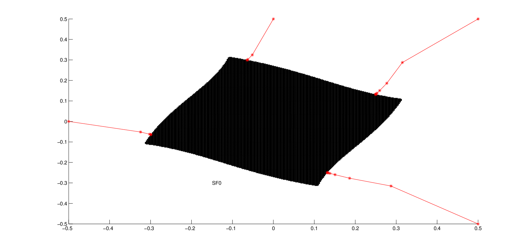
Figure 3: Solution set SF​(0)S_{F}(0) of inclusion (19) and some typical trajectories of the numerical scheme (8).

The following numerical example illustrates that the algorithm (8) indeed approximates an element of the solution set SF​(y¯)S_{F}(\bar{y}) successfully for any given initial value.

Example 12.

Consider the multivalued mapping F:ℝ2→𝒞​𝒞​(ℝ2)F:\mathbbm{R}^{2}\rightarrow\mathcal{CC}(\mathbbm{R}^{2}) given by

F⁡(x)=−3​x+A⁡(x)​Q,F(x)=-3x+A(x)Q, (19)

where

A⁡(x)=(cos⁡(|x|)−sin⁡(|x|)sin⁡(|x|)cos⁡(|x|))andQ=co¯​{(1,0),(0,−1),(−1,0),(0,1)}A(x)=\begin{pmatrix}\cos(|x|)&-\sin(|x|)\\ \sin(|x|)&\cos(|x|)\end{pmatrix}\quad\text{and}\quad Q=\overline{\text{co}}\{(1,0),(0,-1),(-1,0),(0,1)\}

are a rotation matrix with angle depending on the norm of xx and a square centered at the origin. It is easy to check that FF is (−2)(-2)-ROSL and 33-Lipschitz, so that the statements of Proposition 5 hold. The solution set SF​(0)S_{F}(0) and typical trajectories of the numerical method (8) applied to the problem 0∈F⁡(x)0\in F(x) are depicted in Figure 3.

Appendix

The proof of the following proposition does not differ much from that of the classical intermediate value theorem and is therefore omitted.

Proposition 13.

Let a,b∈ℝa,b\in\mathbbm{R} with a<ba<b, and let F:[a,b]→𝒞​𝒞​(ℝ)F:[a,b]\rightarrow\mathcal{CC}(\mathbbm{R}) be an usc mapping such that there exists some fa∈F⁡(a)f_{a}\in F(a) and fb∈F⁡(b)f_{b}\in F(b) with fa<0f_{a}<0 and fb>0f_{b}>0. Then there exists some x∗∈(a,b)x^{*}\in(a,b) such that 0∈F⁡(x∗)0\in F(x^{*}).

References

  • [1] J. P. Aubin and A. Cellina. Differential Inclusions, volume 264 of Grundlehren der mathematischen Wissenschaften. Springer, Berlin, 1984.
  • [2] J.-P. Aubin and H. Frankowska. Set-Valued Analysis. Birkhäuser, Boston, 1990.
  • [3] W.-J. Beyn and J. Rieger. The implicit Euler scheme for one-sided Lipschitz differential inclusions. Discr. Cont. Dyn. Syst. B, 14:409–428, 2010.
  • [4] W.-J. Beyn and J. Rieger. An implicit function theorem for one-sided Lipschitz mappings. Set-Valued and Variational Analysis, 19(3):343–359, 2011.
  • [5] T. Donchev. Qualitative properties of a class of differential inclusions. Glas. Mat. Ser. III, 31(51)(2):269–276, 1996.
  • [6] T. Donchev and E. Farkhi. Stability and Euler approximation of one-sided Lipschitz differential inclusions. SIAM J. Control Optim., 36(2):780–796, 1998.
  • [7] A.L. Dontchev and R.T. Rockafellar. Implicit Functions and Solution Mappings. Springer Monographs in Mathematics. Springer, 2009.