Hidden Parameter Markov Decision Processes: A Semiparametric Regression Approach for Discovering Latent Task Parametrizations
Abstract
Control applications often feature tasks with similar, but not identical, dynamics. We introduce the Hidden Parameter Markov Decision Process (HiP-MDP), a framework that parametrizes a family of related dynamical systems with a low-dimensional set of latent factors, and introduce a semiparametric regression approach for learning its structure from data. In the control setting, we show that a learned HiP-MDP rapidly identifies the dynamics of a new task instance, allowing an agent to flexibly adapt to task variations.
1 Introduction
Many control applications involve repeated encounters with domains that have similar, but not identical, dynamics. An agent swinging a bat may encounter several bats with different weights or lengths, while an agent manipulating a cup may encounter cup with different amounts of liquid. An agent driving a car may encounter many different cars, each with unique handling characteristics.
In all of these scenarios, it makes little sense of the agent to start afresh when it encounters a new bat, a new cup, or a new car. Exposure to a variety of related domains should correspond to faster and more reliable adaptation to a new instance of the same type of domain. If an agent has already swung several bats, for example, we would hope that it could easily learn to swing a new bat. Why? Like many domains, the bat-swinging domain has a low-dimensional representation that affects the system’s dynamics in structured ways. The agent’s prior experience should allow it to both learn how to model related instances of a domain—such as the bat’s length, a latent parameter that smoothly changes in the bat’s dynamics—and what specific model parameters (e.g., lengths) are likely.
Domains with closely-related dynamics are an interesting regime for transfer learning. We introduce the Hidden Parameter Markov Decision Process (HiP-MDP) as a formalization of these types of domains, with two important features. First, we posit that there exist a bounded number of latent parameters that, if known, would fully specify the dynamics. Second, we assume the parameter values remain fixed for a task’s duration (e.g. the bat’s length will not change during a swing), and the agent will know when a change has occurred (getting a new bat).
The HiP-MDP parameters encode the minimum amount of learning required for the agent to adapt to a new domain instance. Given a generative model of how the latent parameters affect domain dynamics, an agent could rapidly identify the dynamics of a particular domain instance by maintaining and updating its distribution (or belief) over the latent parameters. Instead of learning a new policy for each domain instance, it could synthesize a parametrized control policy [1, 2] based on a point estimate of the parameter values, or plan in the belief space over its parameters [3, 4, 5, 6, 7].
We present a method for learning the structure of a HiP-MDP from data. Our generative model uses Indian Buffet Processes [8] to model what latent parameters are relevant for a particular set of dynamics and Gaussian processes [9] to model the dynamics functions. We do not require knowledge of a system’s kinematics equations, nor must we specify the number of latent parameters in advance. Our HiP-MDP model efficiently performs control in the challenging acrobot domain [10] by rapidly identifying the dynamics of new instances.
2 Background
Bayesian Reinforcement Learning
The reinforcement learning setting consists of a series of interactions between an agent and an environment. From some state , the agent chooses an action which transitions it to a new state and provides reward . Its goal is to maximize its longterm expected rewards, , where is a discount factor that weighs the relative importance of near-term and long-term rewards. This series of interactions can be modeled as a Markov Decision Process (MDP), a 5-tuple where and are sets of states and actions , the transition function gives the probability of the next state being after performing action in state , and the reward function gives the reward for performing action in state . We refer to the transition function as the dynamics of a system.
The transition function or the reward function must be learned from experience. Bayesian approaches to reinforcement learning [3, 5, 4] place a prior over the transition function (and sometimes also ), and refine this prior with experience. Thus, the problem of learning an unknown MDP is transformed into a problem of planning in a known partially-observable Markov Decision Process (POMDP). A POMDP [11] consists of a 7-tuple , where and are sets of states , actions , and observations ; and are the transition and reward functions; and the observation function is the probability of receiving an observation when taking action to state . Bayesian RL learns an MDP by planning in a POMDP with states : the fully-observed “world-state” and the hidden dynamics .
However, solving POMDPs in high-dimensional, continuous state spaces remains challenging, despite advances in POMDP planning [4, 12, 6], including situations with mixed-observability [13]. The HiP-MDP, which we introduce in section 3, simplifies the Bayesian RL challenge by using instances of related tasks to first find a low-dimensional representation of the transition function .
Indian Buffet Processes and Gaussian Processes
Our specific instantiation of the HiP-MDP uses two models from Bayesian nonparametric statistics. The first is the Indian Buffet Process (IBP). The IBP is a prior on 0-1 matrices with a potentially unbounded number of columns . To generate samples from the prior, we first use a Beta process to assign a probability to each column such that is bounded. Then, each entry is set to 1 independently with probability . The IBP has the property that the distribution of the number of nonzero columns for any row is , but some columns will be very popular (that is, a few will be large), while others will be used in only a few rows. We will use the IBP as a prior on what latent parameters are relevant for predicting a certain transition output.
The second model we use is the Gaussian Process (GP). A GP is a prior over continuous functions where the prior probability of a set of outputs given a set of inputs is given by a multivariate Gaussian , where is the mean function of the Gaussian process and the covariance matrix has elements for some positive definite kernel function . We use additive mixtures of Gaussian processes to model the transition function.
3 Hidden Parameter Markov Decision Processes
We focus on learning the dynamics and assume that the reward function is fixed across all instances (e.g., the agent always wants to swing the bat). Let denote each instance of a domain. The Hidden Parameter Markov Decision Process (HiP-MDP) posits that the variation in the dynamics of a different instances can be captured through a set of hidden parameters .
The HiP-MDP is be described by a tuple: , where and are the sets of states and actions , and is the reward function. The dynamics for each instance depends on the value of these hidden parameters: . We denote the set of all possible parameters with and let be the prior over these parameters. Thus, a HiP-MDP describes a class of tasks; a particular instance of that class is obtained by fixing the parameter vector . Specifically, we assume that is drawn at the beginning of each task instance and does not change until the beginning of the next instance.
In special cases, we may be able to derive analytic expressions for how affects the dynamics : for example, in a manipulation domain we might be able to derive the kinematic equations of how the cup will respond to a force given a certain volume of liquid. However, in most situations, the simplifications required to derive these analytical forms for the dynamics will be brittle at best. The IBP-GP prior for the HiP-MDP, presented in section 4, describes a semiparametric approach for modeling the dynamics that places few assumptions on the form of the transition function while still maintaining computational tractability.
As pointed out by Bai et al. [7] in a similar setting, we can consider the HiP-MDP a type of POMDP where the hidden state are the parameters . However, a HiP-MDP makes two assumptions which are stronger than those of a POMDP. First, each instance of a HiP-MDP is an MDP—conditioned on the transition and reward functions obey the Markov property. Thus, we could always learn to solve each HiP-MDP instance as its own distinct MDP. Second, the parameter vector is fixed for the duration of the task, and thus the hidden state has no dynamics. This considerably simplifies the procedure for inferring the hidden parametrization.
4 The IBP-GP HiP-MDP
Let the state be some -dimensional vector of continuous, real-valued variables. We propose a transition model of the form:
The weights are the values associated with the latent parameters for instance . The filter parameters denote whether the latent parameter is relevant for making predictions about dimension when taking action . The task-specific basis functions describe how a change in the latent factor affects the dynamics. The additivity assumption in our semi-parametric basis function regression allows us to learn all the latent elements of this model: the number of factors , the weights , the filter parameters , and the form of the basis functions .
Generative Model
The IBP-GP Hip-MDP places the following priors on the three sets of hidden variables, , and :
where and are the parameters of the IBP and GP. Fixing and sets the scale for latent parameters and makes the first basis function the mean dynamics of the domain.
The IBP-GP prior encodes the assumption that for any domain instance the real world contains a countably infinite number of independent scalar latent parameters . However, when making predictions about a specific state dimension given action , only a few of these infinite possible latent parameters will be relevant. Thus, we only need to infer the values of a finite number of weights to characterize the dynamics of a finite number of state dimensions under a finite set of actions. Using an IBP prior on the filter parameters implies that we expect a few latent factors to be relevant for making most of predictions. Moreover, additional prediction tasks—such as a new action, or a new dimension to the state space—can be incorporated consistently. As a regression model, IBP-GP model is an infinite version of the Semiparametric Latent Factor Model [14].
Batch Inference
We focus on scenarios in which the agent is given a large amount of batch observational data from several domain instances and tasked with quickly performing well on new instances. Our batch inference procedure uses the observational data to fit the filter parameters and basis functions , which are independent of any particular instance, and compute a posterior over the weights , which depend on each instance. These settings of , and will used to infer the instance-specific weights efficiently online.
The posterior over the weights is Gaussian given the filter settings and means . However, marginalization over the basis functions requires computing inverses of matrices of size , where is the number of data collected in instance . Instead, we represented each function by a set of pairs for states in a set of support points . Various optimization procedures exist for choosing the support points [15, 14]; we found that iteratively choosing support points from existing points to minimize the maximum reconstruction error within each batch was best for a setting in which a few large errors can result in poor performance.
Given a set of tuples from a task instance , we first created tuples for all and all actions , all dimensions , and all instances . The tuple can be predicted based on all other data available for that action , dimension pair using standard Gaussian process prediction:
where is the collection of tuples with action from instance , is the vector for every , is the matrix , and is the vector of differences . This procedure was repeated for every task instance .
Following this preprocessing step, we proceeded to infer the filter parameters , the weights , and the values of the task-specific basis functions at the support points using a blocked Gibbs sampler. Given and , the posterior over is Gaussian. Let be a column vector of concatenated vectors, and let be a column vector of concatenated vectors. The mean and covariance of is given by
where
where is the Kronecker product, is the matrix for every , and we write to be by matrix of elements such that . We repeat this process for each action and each dimension .
Similarly, given and , the posterior over is also Gaussian. For each instance , the mean and covariance of (that is, the weights not set to zero) are given by:
for , where is matrix with columns concatenating values for for all actions and all dimensions and excluding , and is a column vector concatenating the differences for all actions and all dimensions .
To sample for an already-initialized feature , we note that the likelihood of the model given , , and with some is Gaussian with mean and variance
| (1) | |||||
| (2) |
If , then likelihood is again Gaussian with the same mean (here we assume that the GP prior on is zero-mean) but with covariance
| (3) |
where is a vector of latent parameter values for all instances . We combine these likelihoods with the prior from section 2 to sample .
Initializing a new latent parameter —that is, a for which we do not already have values for the weights —involves computing the marginal likelihood , which is intractable. We approximate the likelihood by sampling sets of new weights . Given values for the weights for each instance , we can compute the likelihood with the new basis function marginalized out using equations 2 and 3. We average these likelihoods to estimate the marginal likelihood of for the new . (For the case, we can just use the variance from equation 2.) If we do set for the new , then samples a set of weights from our samples based on their importance weight (marginal likelihood).
Finally, given the values of the weights for a set of instances , we can update the posterior over with a standard conjugate Gaussian update:
We use this posterior over the weight means when we encounter a new instance .
Online Filtering
Given values for the filter parameters and the basis functions , the posterior on the weights is Gaussian. Thus, we can write the parametrized belief at some time with , where is the inverse covariance and is the information mean . Then the update given an experience tuple is given by
where is a by matrix of basis values , is a by noise matrix with on the diagonal (note that therefore the inverse is trivially computed), and is a -dimensional vector of . If updates are performed only every time steps, we can simply extend , , and to be by , by , and respectively.
Computing requires computing the values of the basis functions at the point . Since we only have the values computed at pseudo-input points , we use our standard GP prediction equation to interpolate the value for this new point:
where is the vector for every , is the matrix , and is the vector . Using only the mean value ignores the uncertainty in the basis function . While incorporating this variance is mathematically straight-forward—all updates remain Gaussian—it adds additional computations to the online calculation. We found that using only the means already provided significant gains in learning in practice.
5 Results
In this section, we describe results on two benchmark problems: cartpole and acrobot [10]. In all of our tests, we use an anisotropic squared-exponential kernel with length and scale parameters approximated for each action and dimension .
5.1 Cartpole
The cartpole task begins with a pole that is initially standing vertically on top of a cart. The agent may apply a force either to the left or the right of the cart to keep the pole from falling over. The domain has a four-dimensional state space consisting of the cart’s position , the cart’s velocity , the pole’s angle , and the pole’s angular velocity . At each time step of length , the system evolves according to the following equations:
| (4) | |||||
where , is the applied force, is gravity, is the mass of both the cart and the pole, and and are the mass and length of the pole, respectively.
| Batch + Train | Batch Only | Train Only | IBP-GP HIP-MDP | |
| 4.8e-06 (1.7e-08) | 4.8e-06 (1.7e-08) | 9.1e-05 (2.3e-07) | 4.7e-06 (1.7e-08) | |
| 1.1e-07 (1.0e-08) | 1.1e-07 (1.1e-08) | 7.6e-07 (1.4e-07) | 3.3e-08 (2.9e-09) | |
| 1.1e-03 (3.2e-06) | 1.1e-03 (3.2e-06) | 3.4e-02 (1.4e-04) | 1.0e-03 (3.2e-06) | |
| 1.5e-05 (1.5e-06) | 1.5e-05 (1.6e-06) | 3.7e-05 (2.8e-06) | 2.5e-06 (1.1e-07) | |
| All | 2.7e-04 (8.9e-04) | 2.7e-04 (8.9e-04) | 8.4e-03 (2.8e-02) | 2.6e-04 (8.8e-04) |
We varied the pole mass and the pole length . Cartpole is a simple enough domain such that changing these parameters does not change the optimal policy—if the pole is falling to the left, the cart should be moved left; if the pole is falling to the right, the cart should be moved right. However, we used cartpole to demonstrate the quality of predictions and describe the latent parameters.
For each training setting, the agent received batches of data from Sarsa [10] (using a rd order Fourier Basis [16]) run for five repetitions of 30 episodes, where each episode was run for 300 iterations or until the pole fell down. Data from seven settings (.1,.4) , (.3,.4) , (.15,.45) , (.2,.55) , (.25,.5) , (.3,.4) , (.3,.6) were reduced to 750 support points and then the batch inference procedure (section 3) was repeated 5 times for 250 iterations with , and the Gaussian process hyper-parameters set from the first batch.
Next, 50 training points were selected from Sarsa run on all settings with and . The online inference procedure (section 3) was used to estimate the weights given the filter parameters and basis functions from the batch procedure. The quality of the predictions was evaluated on 50 (different) test points. Our HiP-MDP predictions were compared to using all of the batch data in a single GP (ignoring the fact that the data came from different instances), using only the 50 training points from the current instance, and combining both the 50 training points and batch data together in one GP.
The relative test log-likelihoods are summarized in figure 1(a), and table 1 summarizes the corresponding mean-squared errors across the 5 runs. Using only the training points from that instance has the highest error across all dimensions , , , and . Our IBP-GP approach performs similarly to just applying a single GP to the batch data for predicting the change in outputs and ; these two dimensions depend only on previous values of and and not on the pole mass or length (see equations 4). Our approach significantly outperforms all baselines for outputs and , whose changes do depend on the parameters of system.
In all 5 of the MCMC runs, a total of 4 latent parameters were inferred. The output dimensions and consistently only used the first (baseline) feature—that is, our IBP-GP’s predictions were in fact the same as using a single GP. This observation is consistent with the cartpole dynamics and the observed prediction errors in figure 1(a) and table 1. The second feature was used by both and and was positively correlated with both the pole mass and the pole length (figures 1(c), 1(b), and 1(b)). In equations 4, both and have many terms. The third consistently discovered feature was used only by and was positively correlated with the pole mass and not correlated with the pole length ; the equations for have several terms that depend only on . The fourth feature (used only to predict ) had the highest variability; it generally has higher values for more extreme length settings, suggesting that it might be a correction for more complex nonlinear effects.

5.2 Acrobot
The acrobot domain features a double-pendulum. The agent can apply a positive, negative, or neutral torque to the joint between the two poles, and its goal is to swing the pendulum up to vertical. The four-dimensional state space consists of the angle and angular velocity of the first segment (with mass ) and the angle and angular velocity of the second segment (with mass ).
For batch training, we used mass settings settings of (.7,.7) , (.7,1.3) , (.9,.7) , (.9,1.1) , (1.1,.9) , (1.1,1.3) , (1.3,.7) , (1.3, 1.3) , again employing Sarsa (this time with a th order Fourier Basis). First, 1000 support points (and GP hyper-parameters) were chosen to minimize the maximum prediction error within each batch. Next, we used the approach in Section 3 to infer the filter parameters and get approximate MAP-estimates for the basis functions .
Table 3 shows mean-squared prediction errors using the same evaluation procedure as cartpole. While the HiP-MDP has slightly higher mean-squared errors on the angle predictions, the IBP-GP approach does better overall and has lower mean-squared errors on the angular velocity predictions. Predicting angular velocities is critical to planning in the acrobot task, as inaccurate predictions will make the agent believe it can reach the swing-up position more quickly than is physically possible.
In acrobat, a policy learned with one mass setting will generally perform poorly on another. For each of the 16 settings with and , we ran 30 repeated trials in which we filtered the weight parameters during an episode and updated the policy at the end of each episode. Even in this “mostly observed” setting, finding the full Bayesian RL solution is PSPACE-complete [17] and offline approximation techniques are an active area of current research [7]. To avoid this complexity, we performed planning using Sarsa with dynamics based on the mean weight parameters . We first obtained an initial value function using the prior mean weights, and then interleaved model-based planning and reinforcement learning, using simulated episodes of planning for each episode of interaction.
Results on acrobot are shown in figure 3. We compare performance (averaged over weight settings) to planning using the true model, and to planning using an average model (learned using all the batch data at once) to obtain an initial value function. Both the average and HiP-MDP model reach performance near, but not quite as high as, using the true model. However, the HiP-MDP model is already near that performance by the nd episode. Using the learned bases from the batches, as well as learning the weights from the first episode, lets it quickly “snap” very near to the true dynamics. By 5 episodes, our IBP-GP model has reached near-optimal performance; the average model takes 15 episodes to reach this level.
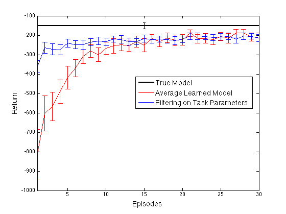 Figure 3: Acrobot performance. The HiP-MDP quickly approaches
near-optimal performance.
Batch + Train
Batch Only
Train Only
IBP-GP HIP-MDP
5.1e-05 (3.1e-06)
5.4e-05 (3.3e-06)
3.8e-04 (3.1e-05)
5.5e-05 (8.3e-06)
1.4e-04 (1.2e-05)
1.5e-04 (1.2e-05)
8.8e-04 (9.6e-05)
1.3e-04 (2.1e-05)
7.0e-04 (4.5e-05)
7.2e-04 (4.8e-05)
1.6e-03 (1.5e-04)
3.6e-04 (4.0e-05)
4.2e-04 (2.5e-05)
4.3e-04 (2.7e-05)
9.1e-04 (1.0e-04)
2.3e-04 (2.1e-05)
All
3.3e-04 (3.8e-05)
3.4e-04 (3.9e-05)
9.4e-04 (8.1e-05)
2.0e-04 (2.1e-05)
Table 4: Mean-Squared Error on Acrobot (with 95% confidence
intervals)
Figure 3: Acrobot performance. The HiP-MDP quickly approaches
near-optimal performance.
Batch + Train
Batch Only
Train Only
IBP-GP HIP-MDP
5.1e-05 (3.1e-06)
5.4e-05 (3.3e-06)
3.8e-04 (3.1e-05)
5.5e-05 (8.3e-06)
1.4e-04 (1.2e-05)
1.5e-04 (1.2e-05)
8.8e-04 (9.6e-05)
1.3e-04 (2.1e-05)
7.0e-04 (4.5e-05)
7.2e-04 (4.8e-05)
1.6e-03 (1.5e-04)
3.6e-04 (4.0e-05)
4.2e-04 (2.5e-05)
4.3e-04 (2.7e-05)
9.1e-04 (1.0e-04)
2.3e-04 (2.1e-05)
All
3.3e-04 (3.8e-05)
3.4e-04 (3.9e-05)
9.4e-04 (8.1e-05)
2.0e-04 (2.1e-05)
Table 4: Mean-Squared Error on Acrobot (with 95% confidence
intervals)
6 Discussion and Related Work
Bai et al. [7] use a very similar hidden-parameter setting treated as a POMDP to perform Bayesian planning; they assume the model is given, whereas our task is to learn it. The HiP-MDP is similar to other POMDPs with fixed hidden states, for example, POMDPs used for slot-filling dialogs [18]. The key difference, however, is that the objective of the HiP-MDP is not simply to gather information (e.g., simply learn the transition function ); it is to perform well on the task (e.g., drive a new car). Transfer learning—the goal of the HiP-MDP—has received much attention in reinforcement learning. Most directly related in spirit to our approach are Hidden-Goal MDPs [17] and hierarchical model-based transfer [19]. In both of these settings, the agent must determine its current MDP from a discrete set of possible MDPs rather than over continuous parameter settings. More related from a technical perspective are representation transfer approaches [20, 21, 22], which typically learn a set of basis functions sufficient for representation any value function defined in a specific state space, or on transfer between two different representations of the same task. By contrast, the HiP-MDP focuses on modeling the dimensions of variation of a family of related tasks.
The IBP-GP prior itself relates to a body of work on multiple-output Gaussian processes (e.g. [23, 14, 24]), though most of these are focused on learning a convolution kernel to model several related outputs on a single task, rather than parameterizing several related tasks. Gaussian process latent variable models [25] have been used for dimensionality reduction in dynamical systems. As with other multi-output GP models, however, GP-LVMs find a time-varying, low-dimensional representation for a single system, while we characterize each instance in a set of systems by a stationary, low-dimensional vector. The focus of these efforts has also been on modeling rather than control.
The extensive work on scaling inference in these Gaussian process models [23, 26, 27] provides several avenues for relaxing some of the approximations that we made in this work (while adding new ones). In settings where one may not have an initial batch of data from several instances, a fully Bayesian treatment of the filter parameters and the basis functions might allow the agent to more accurately navigate its exploration-exploitation trade-offs. Exploring which uncertainties are important to model—and which are not—is an important question for future work. Other extensions within this particular model include applying clustering or more sophisticated hierarchical methods to group together basis functions and thus share statistical strength. For example, one might expect that “opposing actions,” such as in cartpole, could be decomposed into similar basis functions.
7 Conclusion
Machine learning approaches for control often train agents to expect repeated experiences the same domain. However, a more accurate model is that the agent will experience repeated domains that vary in limited and specific ways. In this setting, traditional planning approaches, which typically rely on models, may fail due to the large inter-instance variation. By contrast, reinforcement learning approaches, which typically assume that the dynamics of a new instance are completely unknown, fail to leverage information from related instances.
Our HiP-MDP model explicitly models this inter-instance variation, providing a compromise between these two standard paradigms for control. Our HiP-MDP model will be useful when the family of domains has a parametrization that is small relative to its model and the objectives remains similar across domains. Many applications—such as handling similar objects, driving similar cars, even managing similar network flows—fit this scenario, where batch observational data from related tasks are easy to obtain in advance. In such cases, being able to generalize dynamics from only a few interactions with a new operating regime (using data from many prior interactions with similar systems) is a key step in building controllers that exhibit robust and reliable decision making while gracefully adapting to new situations.
References
- [1] J. Kober, A. Wilhelm, E. Oztop, and J. Peters. Reinforcement learning to adjust parametrized motor primitives to new situations. Autonomous Robots, 33(4):316–379, 2012.
- [2] B.C. da Silva, G.D. Konidaris, and A.G. Barto. Learning parameterized skills. In Proceedings of the Twenty Ninth International Conference on Machine Learning, pages 1679–1686, June 2012.
- [3] P. Poupart, N. Vlassis, J. Hoey, and K. Regan. An analytic solution to discrete Bayesian reinforcement learning. In Twenty-Third International Conference in Machine Learning, pages 697–704, 2006.
- [4] D. Silver and J. Veness. Monte-Carlo planning in large POMDPs. In Advances in Neural Information Processing Systems 23, pages 2164–2172, 2010.
- [5] S. Ross, B. Chaib-draa, and J. Pineau. Bayesian reinforcement learning in continuous POMDPs with application to robot navigation. In The IEEE International Conference on Robotics and Automation, 2008.
- [6] A. Guez, D. Silver, and P. Dayan. Efficient Bayes-adaptive reinforcement learning using sample-based search. In Advances in Neural Information Processing Systems 25, 2012. To appear.
- [7] H. Y. Bai, D. Hsu, and W. S. Lee. Planning how to learn. In International Conference on Robotics and Automation, 2013.
- [8] T.L. Griffiths and Z. Ghahramani. The Indian buffet process: An introduction and review. Journal of Machine Learning Research, 12:1185–1224, 2011.
- [9] C.E. Rasmussen and C.K.I Williams. Gaussian Processes for Machine Learning. The MIT Press, 2005.
- [10] R.S. Sutton and A.G. Barto. Reinforcement Learning: An Introduction. MIT Press, Cambridge, MA, 1998.
- [11] L.P. Kaelbling, M.L. Littman, and A.R. Cassandra. Planning and acting in partially observable stochastic domains. Artificial Intelligence, 101:99–134, 1998.
- [12] H. Kurniawati, D. Hsu, and W.S. Lee. Sarsop: Efficient point-based POMDP planning by approximating optimally reachable belief spaces. In Proceedings of Robotics: Science and Systems, 2008.
- [13] S C W Ong and D Hsu. Planning under uncertainty for robotic tasks with mixed observability. International Journal of Robotics Research, 29(8):1053–1068, 2010.
- [14] Y. W. Teh, M. Seeger, and M. I. Jordan. Semiparametric latent factor models. In International Workshop on Artificial Intelligence and Statistics, 2005.
- [15] E. Snelson and Z. Ghahramani. Sparse Gaussian processes using pseudo-inputs. In Advances in Neural Information Processing Systems 18, 2005.
- [16] G.D. Konidaris, S. Osentoski, and P.S. Thomas. Value function approximation in reinforcement learning using the Fourier basis. In Conference on Artificial Intelligence, pages 380–385, 2011.
- [17] Alan Fern and Prasad Tadepalli. A computational decision theory for interactive assistants. In Advances in Neural Information Processing Systems 23, pages 577–585, 2010.
- [18] J. Williams and S. Young. Scaling up POMDPs for dialogue management: The “summary POMDP” method. In Proceedings of the IEEE ASRU Workshop, 2005.
- [19] A. Wilson, A. Fern, and P. Tadepalli. Transfer learning in sequential decision problems: A hierarchical bayesian approach. Journal of Machine Learning Research - Proceedings Track, 27:217–227, 2012.
- [20] K. Ferguson and S. Mahadevan. Proto-transfer learning in Markov decision processes using spectral methods. In The ICML Workshop on Structural Knowledge Transfer for Machine Learning, June 2006.
- [21] M.E. Taylor and P. Stone. Representation transfer for reinforcement learning. In AAAI 2007 Fall Symposium on Computational Approaches to Representation Change during Learning and Development, November 2007.
- [22] E. Ferrante, A. Lazaric, and M. Restelli. Transfer of task representation in reinforcement learning using policy-based proto-value functions. In Autonomous Agents and Multiagent Systems, pages 1329–1332, 2008.
- [23] M.A. Álvarez and N.D. Lawrence. Computationally efficient convolved multiple output Gaussian processes. Journal of Machine Learning Research, 12:1459–1500, 2011.
- [24] A.G. Wilson, D.A. Knowles, and Z. Ghahramani. Gaussian process regression networks. In Proceedings of the 29th International Conference on Machine Learning, 2012.
- [25] N.D. Lawrence. Gaussian process latent variable models for visualisation of high dimensional data. In Advances in Neural Information Processing Systems 16, 2004.
- [26] M. Titsias. Variational Learning of Inducing Variables in Sparse Gaussian Processes. In the 12th International Conference on Artificial Intelligence and Statistics, volume 5, 2009.
- [27] A.C. Damianou, M.K. Titsias, and N.D. Lawrence. Variational Gaussian process dynamical systems. In Advances in Neural Information Processing Systems 24, 2011.