跳到论文正文
W Papers独立论文阅读器 arXiv:1308.3398 论文正文 计算阅读时间 · 0%
引用这篇论文根据当前论文元数据生成,正式投稿前建议核对。


License: arXiv.org perpetual non-exclusive license
arXiv:1308.3398v2 [hep-th] 19 Nov 2013

KU-TP 060

Higher Derivative Gravity and Asymptotic Safety
in Diverse Dimensions

Nobuyoshi Ohta11 1 e-mail address: ohtan@phys.kindai.ac.jp,a and Roberto Percacci22 2 e-mail address: percacci@sissa.it,b,c

aDepartment of Physics, Kinki University, Higashi-Osaka, Osaka 577-8502, Japan

bInternational School for Advanced Studies, via Bonomea 265, 34136 Trieste, Italy

cINFN, Sezione di Trieste, Italy

Abstract

We derive the one-loop beta functions for a theory of gravity with generic action containing up to four derivatives. The calculation is done in arbitrary dimension and on an arbitrary background. The special cases of three, four, near four, five and six dimensions are discussed in some detail. In all these dimensions there are nontrivial UV fixed points, which mean that within the approximations there are asymptotically safe trajectories. We also find an indication that a Weyl-invariant fixed point exists in four dimensions. The new massive gravity in three dimensions does not correspond to a fixed point.

1 Introduction

The empirical success of Einstein’s theory of gravity does not imply that the gravitational action must contain only the Hilbert term, nor that any other terms must be “small”. For example, consider terms quadratic in curvature. Neglecting indices and setting the cosmological constant to zero, the Lagrangian will be of the form

ℒ=mP2​R+c​R2,\displaystyle{\cal L}=m_{P}^{2}R+cR^{2}\ , (1.1)

where mPm_{P} is the Planck mass, “R2R^{2}” stands for generic quadratic combinations of curvature tensors and cc stands for dimensionless couplings. In the weak field limit we can expand around flat space and write in momentum space

ℒ=mP2​p2+c​p4.\displaystyle{\cal L}=m_{P}^{2}p^{2}+cp^{4}\ . (1.2)

The agreement of Einstein’s theory with observation puts bounds on the cc’s: c≪(mP/p)2c\ll(m_{P}/p)^{2}. The strongest bound comes the highest momenta. From the validity of Newton’s law in the millimeter range, one gets the bound c≪1062c\ll 10^{62}. This ridiculously weak bound is just a consequence of our inability of testing gravity at high energy, and is another way of seeing how good the effective field theory of gravity really is [1, 2]. If one believes that gravity must be described by some quantum theory at some level, then the logic of effective field theories leads us to expect that ℒ{\cal L} will contain terms quadratic in curvatures, with coefficients cc presumably of order unity. In fact, one expects to find in the action all possible diffeomorphism–invariant terms constructed with the metric and its derivatives.

In this non-renormalizable effective field theory of gravity, the expansion parameter is p/mP=p​G=G~p/m_{P}=p\sqrt{G}=\tilde{G}, the propagator is given by the Einstein–Hilbert term and higher derivative terms can be treated as perturbations. On the other hand, it had been shown long ago that if one uses as propagator the inverse of (1.2), then the theory is perturbatively renormalizable [3]. The price one pays is that perturbative unitarity is lost. More precisely, if the coefficients cc are chosen so as to make the theory renormalizable, there is an unphysical ghost state, and if the coefficients cc are such that there is no ghost, the theory is not renormalizable. Several possible ways out of this dilemma have been proposed, and we will mention some later on. Here we would like to point out that even when this theory is renormalizable, it is not UV complete, because Newton’s constant is an irrelevant coupling and G~\tilde{G} blows up. The only way it could be UV complete is if G~\tilde{G} tended to a finite limit, in other words if there was a fixed point (FP). This is called asymptotic safety [4].

The beta functions for higher derivative gravity in four dimensions have been calculated at one loop long ago. After some early attempts [5, 6], the correct beta functions for the dimensionless couplings cc have been obtained by Avramidi and Barvinsky [7]. The calculation has been reviewed and extended to 4−ϵ4-\epsilon dimensions in [8, 9]. The running of Newton’s constant and of the cosmological constant were also derived, but only taking into account the contribution from the universal logarithmically divergent terms (or equivalently, in dimensional regularization, from the simple pole at D=4D=4). The non-universal terms, corresponding to quadratic and quartically divergent terms in the effective action, were calculated later in [10, 11] and they were shown to lead to a FP for Newton’s constant and for the cosmological constant. The calculation was repeated using different techniques (and hence with slightly different results for the non-universal part) in [12, 13]. Some calculations that go beyond the one-loop approximation have been performed in [14, 15], and find also for the cc coefficients a finite but nonzero FP value. The significance of this result is not entirely clear at the moment.

Higher derivative gravity is an interesting subject also in three dimensions, where Einstein theory is trivial (in the sense that it does not have any propagating degrees of freedom). If one adds to the Einstein–Hilbert action a Chern–Simons term, which contains three derivatives, then it contains a propagating massive graviton whose helicity depends on the sign of the “topological mass” [16]. The renormalization group (RG) of this “topologically massive gravity” has been studied in [17], and its supergravity extension in [18].

These theories, however, violate parity. More recently it has been shown that the addition of specific four-derivative terms to three-dimensional gravity (with wrong sign of Einstein–Hilbert term) makes the theory unitary [19]. The addition of these terms introduces propagating massive graviton around flat Minkowski and curved maximally symmetric spacetimes (anti-de Sitter (AdS) and de Sitter (dS) spacetimes). In contrast to topologically massive gravity, this so–called “new massive gravity” preserves parity. This is very interesting in that we have really dynamical theory of gravity that is unitary even though higher derivative terms are included. Various aspects of this theory have been later investigated. Linearized excitations in the field equations were studied in [20]. Unitarity is proven for Minkowski spacetime in [21, 22, 23], whereas it is discussed in [24] for maximally symmetric spacetimes. A complete classification of the unitary theories for the most general action with arbitrary coefficients of all possible terms is given in [25]. The partial result of unitarity condition on the flat Minkowski spacetime was known for the usual sign of the Einstein theory [26]. Unfortunately, the new massive gravity turned out to be non-renormalizable though the general theory with arbitrary coefficients for the quadratic curvature terms is renormalizable [22, 27, 28]. As in the four–dimensional case, perturbative renormalizability is not sufficient for UV completeness. For that, a FP is needed.

To establish whether new massive gravity, or some other three–dimensional gravity theory, has a nontrivial FP, it is necessary to study its beta functions. It is well known that Einstein gravity, in spite of not having any propagating degrees of freedom, has such a FP, and it was shown in [17] that also topologically massive gravity does. Much less is known in the case when four–derivative terms are present. The running of Newton’s constant and of the cosmological constant has been studied in [29] and it has been shown that it has a FP with the desired properties, but the running of the four–derivative couplings has not been studied so far. One of the main motivations of this paper is to derive the RG flow of generic four–derivative gravities in three dimensions. The main questions are whether a FP exists (we will see that it does) and whether the special ratio of couplings that defines new massive gravity is stable under RG flow (it is not).

Since the derivation of the beta functions changes little in different dimensions, we will perform most of the calculations in arbitrary dimension and discuss in detail only the cases D=4D=4 and D=3D=3, with additional results for D=5D=5 and 6.

This paper is organized as follows. In sect. 2, we summarize the gravity theory we consider with the Einstein term, cosmological constant and quadratic curvatures, and give definitions of coupling constants. In sect. 3, we give quadratic expansion of the action necessary for our calculation of beta functions. In sect. 4, we give derivation of the beta functions from functional renormalization group equation (FRGE) in arbitrary dimensions. Though we have the results on beta functions for arbitrary dimensions, they are very complicated and the explicit form is not so illuminating. So in sects. 5 to 9, we discuss the beta functions and their fixed points explicitly only for dimensions 4, near 4, 3, 5 and 6, respectively, and show that the theories have nontrivial UV FPs and are asymptotically safe in all these dimensions. By analysing beta functions near four dimensions, we find an indication that Weyl-invariant FP exists in four dimensions. We also find that the new massive gravity does not correspond to any FP. Sect. 10 is devoted to our conclusions.

2 Four–derivative Gravity

We will consider actions of the general form

S=∫dD​x​−g​[1κ2​(σ​R−2​Λ)+α​R2+β​Rμ​ν2+γ​Rμ​ν​ρ​λ2],\displaystyle S=\int d^{D}x\sqrt{-g}\Big[\frac{1}{\kappa^{2}}(\sigma R-2\Lambda)+\alpha R^{2}+\beta R_{\mu\nu}^{2}+\gamma R_{\mu\nu\rho\lambda}^{2}\Big], (2.1)

where κ2=16​π​G\kappa^{2}=16\pi G is the DD-dimensional gravitational constant, σ=±1\sigma=\pm 1 is the sign of the Hilbert action, Λ\Lambda is the cosmological constant, α\alpha, β\beta, γ\gamma are the higher derivative couplings. It is sometimes more convenient to use a different basis for the higher derivative terms, namely R2R^{2}, the square of the Weyl tensor

C2=Rμ​ν​α​β2−4D−2​Rμ​ν2+2(D−1)​(D−2)​R2,\displaystyle C^{2}=R_{\mu\nu\alpha\beta}^{2}-\frac{4}{D-2}R_{\mu\nu}^{2}+\frac{2}{(D-1)(D-2)}R^{2}, (2.2)

and the Gauss–Bonnet combination

E=Rμ​ν​α​β2−4​Rμ​ν2+R2,\displaystyle E=R_{\mu\nu\alpha\beta}^{2}-4R_{\mu\nu}^{2}+R^{2}, (2.3)

which is topological for D=4D=4 and vanishes identically for D=3D=3. Then the action has the alternative form

S=∫dD​x​−g​[1κ2​(σ​R−2​Λ)+12​λ​C2−1ρ​E+1ξ​R2+τ​□​R],\displaystyle S=\int d^{D}x\sqrt{-g}\Big[\frac{1}{\kappa^{2}}(\sigma R-2\Lambda)+\frac{1}{2\lambda}C^{2}-\frac{1}{\rho}E+\frac{1}{\xi}R^{2}+\tau\Box R\Big], (2.4)

where

λ=2​(D−3)(D−2)​(β+4​γ),ρ=4​(D−3)(D−2)​β+4​γ,ξ=−4​(D−1)4​(D−1)​α+D​β+4​γ.\displaystyle\lambda=\frac{2(D-3)}{(D-2)(\beta+4\gamma)},~~\rho=\frac{4(D-3)}{(D-2)\beta+4\gamma},~~\xi=-\frac{4(D-1)}{4(D-1)\alpha+D\beta+4\gamma}\ . (2.5)

or conversely

α=−1ρ+1ξ+1(D−1)​(D−2)​λ,β=4ρ−2(D−2)​λ,γ=−1ρ+12​λ.\displaystyle\alpha=-\frac{1}{\rho}+\frac{1}{\xi}+\frac{1}{(D-1)(D-2)\lambda},~~\beta=\frac{4}{\rho}-\frac{2}{(D-2)\lambda},~~\gamma=-\frac{1}{\rho}+\frac{1}{2\lambda}. (2.6)

Note that in D=3D=3, C2C^{2} and EE both vanish identically and the form (2.4) is not appropriate. The couplings λ\lambda, ρ\rho and ξ\xi have mass dimension 4−D4-D. In dimensions higher than three, it is customary to define the dimensionless combinations

ω≡−(D−1)​λξ,θ≡λρ.\displaystyle\omega\equiv-\frac{(D-1)\lambda}{\xi},~~~\theta\equiv\frac{\lambda}{\rho}\ . (2.7)

Our conventions are summarized in Appendix A.

The variation of each term gives the field equations:

σ​Gμ​ν+Λ​gμ​ν+κ2​(α​Eμ​ν(1)+β​Eμ​ν(2)+γ​Eμ​ν(3))=0,\displaystyle\sigma G_{\mu\nu}+\Lambda g_{\mu\nu}+\kappa^{2}(\alpha E_{\mu\nu}^{(1)}+\beta E_{\mu\nu}^{(2)}+\gamma E_{\mu\nu}^{(3)})=0, (2.8)

where Gμ​νG_{\mu\nu} is the Einstein tensor and

Eμ​ν(1)\displaystyle E_{\mu\nu}^{(1)} =\displaystyle= 2​R​Rμ​ν−2​∇μ​∇νR+gμ​ν​(2​□​R−12​R2),\displaystyle 2RR_{\mu\nu}-2\nabla_{\mu}\nabla_{\nu}R+g_{\mu\nu}\Big(2\Box R-\frac{1}{2}R^{2}\Big),
Eμ​ν(2)\displaystyle E_{\mu\nu}^{(2)} =\displaystyle= 2​Rμ​λ​Rνλ−2​∇λ​∇(μCLOSEROPENν)​λ+□​Rμ​ν+12​(□​R−Rλ​ρ2)​gμ​ν,\displaystyle 2R_{\mu\lambda}R_{\nu}^{\lambda}-2\nabla^{\lambda}\nabla_{(\mu}R_{\nu)\lambda}+\Box R_{\mu\nu}+\frac{1}{2}(\Box R-R_{\lambda\rho}^{2})g_{\mu\nu},
Eμ​ν(3)\displaystyle E_{\mu\nu}^{(3)} =\displaystyle= 2Rμ​ρ​λ​σRνρ​λ​σ+4∇(ρCLOSE∇OPENλ)Rμρνλ−12gμ​νRρ​λ​σ​τ2.\displaystyle 2R_{\mu\rho\lambda\sigma}R_{\nu}{}^{\rho\lambda\sigma}+4\nabla_{(\rho}\nabla_{\lambda)}R_{\mu}{}^{\rho}{}_{\nu}{}^{\lambda}-\frac{1}{2}g_{\mu\nu}R_{\rho\lambda\sigma\tau}^{2}. (2.9)

3 Quadratic expansion of the action

We will apply the standard background field method, expanding the metric as

gμ​ν=g¯μ​ν+hμ​ν.\displaystyle g_{\mu\nu}=\bar{g}_{\mu\nu}+h_{\mu\nu}\ . (3.1)

In order to derive the effective action at the one-loop level, or to calculate the one-loop beta functions, we need the expansion of the action to second order in hμ​νh_{\mu\nu}. This calculation is discussed in detail in Appendix B. The most complicated part comes from the expansion of the terms quadratic in curvature. We report here the final form, where we have dropped terms with linear derivatives acting on the fluctuation and terms with two derivatives acting on a background curvature (omitting indices, these are of the form h(∇R¯)∇hh(\nabla\bar{R})\nabla h and h(∇∇R¯)hh(\nabla\nabla\bar{R})h; such terms do not contribute to the final results, see for example [7, 9]). The terms proportional to α\alpha can be written in the form

αhμ​ν[∇μ∇ν∇α∇β−g¯μ​ν□∇α∇β−g¯α​β∇μ∇ν□+g¯μ​νg¯α​β□2−R¯g¯ν​β∇α∇μ\displaystyle\alpha h^{\mu\nu}\Big[\nabla_{\mu}\nabla_{\nu}\nabla_{\alpha}\nabla_{\beta}-\bar{g}_{\mu\nu}\Box\nabla_{\alpha}\nabla_{\beta}-\bar{g}_{\alpha\beta}\nabla_{\mu}\nabla_{\nu}\Box+\bar{g}_{\mu\nu}\bar{g}_{\alpha\beta}\Box^{2}-\bar{R}\bar{g}_{\nu\beta}\nabla_{\alpha}\nabla_{\mu}
−(2​R¯μ​ν−R¯​g¯μ​ν)​∇α∇β+2​R¯μ​ν​g¯α​β​□+12​R¯​(g¯μ​α​g¯ν​β−g¯μ​ν​g¯α​β)​□−R¯​R¯α​β​g¯μ​ν\displaystyle-(2\bar{R}_{\mu\nu}-\bar{R}\bar{g}_{\mu\nu})\nabla_{\alpha}\nabla_{\beta}+2\bar{R}_{\mu\nu}\bar{g}_{\alpha\beta}\Box+\frac{1}{2}\bar{R}(\bar{g}_{\mu\alpha}\bar{g}_{\nu\beta}-\bar{g}_{\mu\nu}\bar{g}_{\alpha\beta})\Box-\bar{R}\bar{R}_{\alpha\beta}\bar{g}_{\mu\nu}
+2R¯R¯μ​αg¯β​ν+R¯μ​νR¯α​β−14Jμ​ν​α​βR¯2]hα​β.\displaystyle+2\bar{R}\bar{R}_{\mu\alpha}\bar{g}_{\beta\nu}+\bar{R}_{\mu\nu}\bar{R}_{\alpha\beta}-\frac{1}{4}J_{\mu\nu\alpha\beta}\bar{R}^{2}\Big]h^{\alpha\beta}\ . (3.2)

Here and in what follows, a bar indicates that the quantity is evaluated on the background; the indices are raised, lowered and contracted by the background metric g¯\bar{g}, the covariant derivative ∇\nabla is constructed with the background metric. The tensor JJ is defined by

Jμ​ν​α​β=δμ​ν,α​β−12​g¯μ​ν​g¯α​β\displaystyle J_{\mu\nu\alpha\beta}=\delta_{\mu\nu,\alpha\beta}-\frac{1}{2}\bar{g}_{\mu\nu}\bar{g}_{\alpha\beta} (3.3)

where

δμ​ν,α​β=12​(g¯μ​α​g¯ν​β+g¯μ​β​g¯ν​α)≡1^,\displaystyle\delta_{\mu\nu,\alpha\beta}=\frac{1}{2}(\bar{g}_{\mu\alpha}\bar{g}_{\nu\beta}+\bar{g}_{\mu\beta}\bar{g}_{\nu\alpha})\equiv\hat{1}, (3.4)

is the identity in the space of symmetric tensors. We should note that due to the presence of the external factors of hh, the expression in the square bracket is automatically symmetrized under the interchanges μ↔ν\mu\leftrightarrow\nu, α↔β\alpha\leftrightarrow\beta and (μ,ν)↔(α,β)(\mu,\nu)\leftrightarrow(\alpha,\beta).

The β\beta terms can be written in the form

β​hμ​ν\displaystyle\beta h^{\mu\nu}\hskip-19.91692pt [12∇μ∇ν∇α∇β−12g¯μ​ν∇α□∇β−12g¯ν​β∇μ□∇α+14(g¯μ​αg¯ν​β+g¯μ​νg¯α​β)□2+12R¯ν​β∇α∇μ\displaystyle\Big[\frac{1}{2}\nabla_{\mu}\nabla_{\nu}\nabla_{\alpha}\nabla_{\beta}-\frac{1}{2}\bar{g}_{\mu\nu}\nabla_{\alpha}\Box\nabla_{\beta}-\frac{1}{2}\bar{g}_{\nu\beta}\nabla_{\mu}\Box\nabla_{\alpha}+\frac{1}{4}(\bar{g}_{\mu\alpha}\bar{g}_{\nu\beta}+\bar{g}_{\mu\nu}\bar{g}_{\alpha\beta})\Box^{2}+\frac{1}{2}\bar{R}_{\nu\beta}\nabla_{\alpha}\nabla_{\mu} (3.5)
−2​R¯μρ​g¯ν​β​∇ρ∇α+32​g¯α​β​R¯ρ​μ​∇ρ∇ν+R¯μ​α​ν​β​□+14​(2​g¯μ​α​g¯ν​β−g¯μ​ν​g¯α​β)​R¯ρ​λ​∇ρ∇λ−32​R¯βρ​R¯ρ​μ​ν​α\displaystyle-2\bar{R}_{\mu}^{\rho}\bar{g}_{\nu\beta}\nabla_{\rho}\nabla_{\alpha}+\frac{3}{2}\bar{g}_{\alpha\beta}\bar{R}_{\rho\mu}\nabla^{\rho}\nabla_{\nu}+\bar{R}_{\mu\alpha\nu\beta}\Box+\frac{1}{4}(2\bar{g}_{\mu\alpha}\bar{g}_{\nu\beta}-\bar{g}_{\mu\nu}\bar{g}_{\alpha\beta})\bar{R}^{\rho\lambda}\nabla_{\rho}\nabla_{\lambda}-\frac{3}{2}\bar{R}^{\rho}_{\beta}\bar{R}_{\rho\mu\nu\alpha}
+R¯μ​ρ​λ​νR¯α+ρ​λβ12g¯ν​βR¯μ​ρR¯αρ−g¯α​βR¯μ​ρR¯νρ−14Jμ​ν​α​βR¯ρ​σ2]hα​β,\displaystyle+\bar{R}_{\mu\rho\lambda\nu}\bar{R}_{\alpha}{}^{\rho\lambda}{}_{\beta}+\frac{1}{2}\bar{g}_{\nu\beta}\bar{R}_{\mu\rho}\bar{R}^{\rho}_{\alpha}-\bar{g}_{\alpha\beta}\bar{R}_{\mu\rho}\bar{R}^{\rho}_{\nu}-\frac{1}{4}J_{\mu\nu\alpha\beta}\bar{R}_{\rho\sigma}^{2}\Big]h^{\alpha\beta}\ ,

and the terms proportional to γ\gamma are

γ​hμ​ν\displaystyle\gamma h^{\mu\nu}\hskip-14.22636pt [∇μ∇ν∇α∇β+g¯μ​αg¯ν​β□2−2g¯ν​β∇μ□∇α−2g¯ν​βR¯μ​ρ​λ​α∇ρ∇λ+3R¯μ​α​ν​β□\displaystyle\hskip-5.69054pt\Big[\nabla_{\mu}\nabla_{\nu}\nabla_{\alpha}\nabla_{\beta}+\bar{g}_{\mu\alpha}\bar{g}_{\nu\beta}\Box^{2}-2\bar{g}_{\nu\beta}\nabla_{\mu}\Box\nabla_{\alpha}-2\bar{g}_{\nu\beta}\bar{R}_{\mu\rho\lambda\alpha}\nabla^{\rho}\nabla^{\lambda}+3\bar{R}_{\mu\alpha\nu\beta}\Box (3.6)
−4​R¯μ​α​ρ​ν​∇ρ∇β−4​g¯ν​β​R¯ρ​μ​∇ρ∇α−2​g¯ν​β​R¯μ​α​□+g¯μ​α​g¯ν​β​R¯ρ​λ​∇ρ∇λ\displaystyle-4\bar{R}_{\mu\alpha\rho\nu}\nabla^{\rho}\nabla_{\beta}-4\bar{g}_{\nu\beta}\bar{R}_{\rho\mu}\nabla^{\rho}\nabla_{\alpha}-2\bar{g}_{\nu\beta}\bar{R}_{\mu\alpha}\Box+\bar{g}_{\mu\alpha}\bar{g}_{\nu\beta}\bar{R}_{\rho\lambda}\nabla^{\rho}\nabla^{\lambda}
−2g¯μ​νR¯ρ​α​λ​β∇λ∇ρ+4R¯μ​α∇ν∇β+2g¯ν​βR¯μ​λ​ρ​σR¯αλ​ρ​σ−2g¯ν​βR¯ρ​λR¯μ​ρ​α​λ\displaystyle-2\bar{g}_{\mu\nu}\bar{R}_{\rho\alpha\lambda\beta}\nabla^{\lambda}\nabla^{\rho}+4\bar{R}_{\mu\alpha}\nabla_{\nu}\nabla_{\beta}+2\bar{g}_{\nu\beta}\bar{R}_{\mu\lambda\rho\sigma}\bar{R}_{\alpha}{}^{\lambda\rho\sigma}-2\bar{g}_{\nu\beta}\bar{R}^{\rho\lambda}\bar{R}_{\mu\rho\alpha\lambda}
−R¯μ​λ​ρ​βR¯νρ​λα+3R¯μ​αρ​λR¯ν​ρ​β​λ−3R¯μ​λ​ν​ρR¯αρ​λβ−3R¯ραR¯μ​β​ν​ρ\displaystyle-\bar{R}_{\mu\lambda\rho\beta}\bar{R}_{\nu}{}^{\rho\lambda}{}_{\alpha}+3\bar{R}_{\mu\alpha}{}^{\rho\lambda}\bar{R}_{\nu\rho\beta\lambda}-3\bar{R}_{\mu\lambda\nu\rho}\bar{R}_{\alpha}{}^{\rho\lambda}{}_{\beta}-3\bar{R}^{\rho}_{\alpha}\bar{R}_{\mu\beta\nu\rho}
+2R¯μ​αR¯ν​β−g¯μ​νR¯αR¯β​ρ​λ​σρ​λ​σ−14Jμ​ν​α​βR¯ρ​σ​λ​τ2]hα​β.\displaystyle+2\bar{R}_{\mu\alpha}\bar{R}_{\nu\beta}-\bar{g}_{\mu\nu}\bar{R}_{\alpha}{}^{\rho\lambda\sigma}\bar{R}_{\beta\rho\lambda\sigma}-\frac{1}{4}J_{\mu\nu\alpha\beta}\bar{R}_{\rho\sigma\lambda\tau}^{2}\Big]h^{\alpha\beta}.

It can be checked that when arranged in the Gauss-Bonnet combination (γ=α\gamma=\alpha, β=−4​α\beta=-4\alpha) and the background metric is maximally symmetric, one obtains a total derivative. This gives a nontrivial check of the results.

The BRST transformation for the fields is found to be

δB​gμ​ν\displaystyle\delta_{B}g_{\mu\nu}\hskip-5.69054pt =\displaystyle= −δ​λ​[gρ​ν​∇μcρ+gρ​μ​∇νcρ]≡−δ​λ​𝒟μ​ν,ρ​cρ,\displaystyle\hskip-5.69054pt-\delta\lambda[g_{\rho\nu}\nabla_{\mu}c^{\rho}+g_{\rho\mu}\nabla_{\nu}c^{\rho}]\equiv-\delta\lambda{\cal D}_{\mu\nu,\rho}c^{\rho},
δB​cμ\displaystyle\delta_{B}c^{\mu}\hskip-5.69054pt =\displaystyle= −δ​λ​cρ​∇ρcμ,δB​c¯μ=i​δ​λ​Bμ,δB​Bμ=0,\displaystyle\hskip-5.69054pt-\delta\lambda c^{\rho}\nabla_{\rho}c^{\mu},~~~\delta_{B}\bar{c}_{\mu}=i\delta\lambda\,B_{\mu},~~~\delta_{B}B_{\mu}=0, (3.7)

which is nilpotent. Here cμ,c¯μc^{\mu},\bar{c}_{\mu} and BμB_{\mu} are the Faddeev-Popov ghost, anti-ghost and an auxiliary field, respectively, and δ​λ\delta\lambda is an anticommuting parameter. The gauge fixing term and the Faddeev-Popov ghost terms are concisely written as

ℒG​F+F​P/−g¯\displaystyle{\cal L}_{GF+FP}/\sqrt{-\bar{g}}\hskip-5.69054pt =\displaystyle= i​δB​[c¯μ​Yμ​ν​(χν−a2​Bν)]/δ​λ\displaystyle\hskip-5.69054pti\delta_{B}[\bar{c}_{\mu}Y^{\mu\nu}(\chi_{\nu}-\frac{a}{2}B_{\nu})]/\delta\lambda (3.8)
=\displaystyle= −Bμ​Yμ​ν​χν+i​c¯μ​Yμ​ν​(∇λ𝒟λ​ν,ρ+b​∇ν𝒟λ,ρλ)​cρ+a2​Bμ​Yμ​ν​Bν\displaystyle\hskip-5.69054pt-B_{\mu}Y^{\mu\nu}\chi_{\nu}+i\bar{c}_{\mu}Y^{\mu\nu}(\nabla^{\lambda}{\cal D}_{\lambda\nu,\rho}+b\nabla_{\nu}{\cal D}_{\lambda,\rho}^{\lambda})c^{\rho}+\frac{a}{2}B_{\mu}Y^{\mu\nu}B_{\nu}
≃\displaystyle\simeq −12​a​χμ​Yμ​ν​χν+i​c¯μ​Yμ​ν​[gν​ρ​□+(2​b+1)​∇ν∇ρ+R¯ν​ρ]​cρ,\displaystyle-\frac{1}{2a}\chi_{\mu}Y^{\mu\nu}\chi_{\nu}+i\bar{c}_{\mu}Y^{\mu\nu}[g_{\nu\rho}\Box+(2b+1)\nabla_{\nu}\nabla_{\rho}+\bar{R}_{\nu\rho}]c^{\rho},

where the auxiliary field BμB_{\mu} is integrated out in the last line. Here

χμ\displaystyle\chi_{\mu} ≡\displaystyle\equiv ∇λhλ​μ+b​∇μh,\displaystyle\nabla^{\lambda}h_{\lambda\mu}+b\nabla_{\mu}h,
Yμ​ν\displaystyle Y_{\mu\nu} ≡\displaystyle\equiv g¯μ​ν​□+c​∇μ∇ν−d​∇ν∇μ.\displaystyle\bar{g}_{\mu\nu}\Box+c\nabla_{\mu}\nabla_{\nu}-d\nabla_{\nu}\nabla_{\mu}. (3.9)

where aa, bb, cc and dd are gauge parameters. We choose them such that the non-minimal four derivative terms ∇μ∇ν​∇α∇β\nabla_{\mu}\nabla_{\nu}\nabla_{\alpha}\nabla_{\beta}, g¯μ​ν​□​∇α∇β\bar{g}_{\mu\nu}\Box\nabla_{\alpha}\nabla_{\beta} and g¯ν​β​∇μ□​∇α\bar{g}_{\nu\beta}\nabla_{\mu}\Box\nabla_{\alpha} cancel. This leads to the choice [9]

a=1β+4​γ,b=4​α+β4​(γ−α),c−d=2​(γ−α)β+4​γ−1.\displaystyle a=\frac{1}{\beta+4\gamma},~~~b=\frac{4\alpha+\beta}{4(\gamma-\alpha)},~~~c-d=\frac{2(\gamma-\alpha)}{\beta+4\gamma}-1. (3.10)

In order to simplify the gauge-fixing term, we will further choose d=1d=1. With these choices, the ghost operator is

Δg​h=δμ□ν+(1+2b)∇μ∇ν+R¯μ.ν\displaystyle\Delta_{gh}=\delta^{\mu}{}_{\nu}\Box+(1+2b)\nabla_{\mu}\nabla^{\nu}+\bar{R}^{\mu}{}_{\nu}\ . (3.11)

Then, the quadratic terms in the action can be written in the form hμ​ν​𝒦μ​ν,α​β​hα​βh^{\mu\nu}{\cal K}_{\mu\nu,\alpha\beta}h^{\alpha\beta}, where

𝒦=K​□2+Dρ​λ​∇ρ∇λ+W.\displaystyle{\cal K}=K\Box^{2}+D_{\rho\lambda}\nabla^{\rho}\nabla^{\lambda}+W. (3.12)

The explicit forms of the coefficients are

(K)μ​ν,α​β=β+4​γ4​(g¯μ​α​g¯ν​β+4​α+β4​(γ−α)​g¯μ​ν​g¯α​β),\displaystyle(K)_{\mu\nu,\alpha\beta}=\frac{\beta+4\gamma}{4}\Big(\bar{g}_{\mu\alpha}\bar{g}_{\nu\beta}+\frac{4\alpha+\beta}{4(\gamma-\alpha)}\bar{g}_{\mu\nu}\bar{g}_{\alpha\beta}\Big), (3.13)
(Dρ​λ)μ​ν,α​β\displaystyle(D_{\rho\lambda})_{\mu\nu,\alpha\beta}\hskip-5.69054pt =\displaystyle= −2​γ​g¯ν​β​R¯α​ρ​λ​μ+4​γ​g¯ρ​ν​R¯λ​α​μ​β+(β+3​γ)​g¯ρ​λ​R¯μ​α​ν​β−(2​β+4​γ)​g¯α​ρ​g¯ν​β​R¯μ​λ\displaystyle\hskip-5.69054pt-2\gamma\bar{g}_{\nu\beta}\bar{R}_{\alpha\rho\lambda\mu}+4\gamma\bar{g}_{\rho\nu}\bar{R}_{\lambda\alpha\mu\beta}+(\beta+3\gamma)\bar{g}_{\rho\lambda}\bar{R}_{\mu\alpha\nu\beta}-(2\beta+4\gamma)\bar{g}_{\alpha\rho}\bar{g}_{\nu\beta}\bar{R}_{\mu\lambda} (3.14)
−2​γ​g¯ν​β​R¯μ​α​g¯ρ​λ+β​g¯μ​ν​g¯β​ρ​R¯α​λ−2​α​g¯α​ρ​g¯β​λ​R¯μ​ν+2​α​g¯μ​ν​g¯ρ​λ​R¯α​β+2​γ​g¯μ​ν​R¯α​ρ​λ​β\displaystyle\hskip-5.69054pt-2\gamma\bar{g}_{\nu\beta}\bar{R}_{\mu\alpha}\bar{g}_{\rho\lambda}+\beta\bar{g}_{\mu\nu}\bar{g}_{\beta\rho}\bar{R}_{\alpha\lambda}-2\alpha\bar{g}_{\alpha\rho}\bar{g}_{\beta\lambda}\bar{R}_{\mu\nu}+2\alpha\bar{g}_{\mu\nu}\bar{g}_{\rho\lambda}\bar{R}_{\alpha\beta}+2\gamma\bar{g}_{\mu\nu}\bar{R}_{\alpha\rho\lambda\beta}
+(α2​R¯+σ4​κ2)​(g¯μ​α​g¯ν​β​g¯ρ​λ−g¯μ​ν​g¯α​β​g¯ρ​λ−2​g¯ν​β​g¯μ​ρ​g¯α​λ+2​g¯μ​ν​g¯α​ρ​g¯β​λ)\displaystyle\hskip-5.69054pt+\Big(\frac{\alpha}{2}\bar{R}+\frac{\sigma}{4\kappa^{2}}\Big)(\bar{g}_{\mu\alpha}\bar{g}_{\nu\beta}\bar{g}_{\rho\lambda}-\bar{g}_{\mu\nu}\bar{g}_{\alpha\beta}\bar{g}_{\rho\lambda}-2\bar{g}_{\nu\beta}\bar{g}_{\mu\rho}\bar{g}_{\alpha\lambda}+2\bar{g}_{\mu\nu}\bar{g}_{\alpha\rho}\bar{g}_{\beta\lambda})
+2​γ​g¯ν​ρ​g¯β​λ​R¯μ​α+(β2+γ)​g¯μ​α​g¯ν​β​R¯ρ​λ−β4​g¯μ​ν​g¯α​β​R¯ρ​λ,\displaystyle\hskip-5.69054pt+2\gamma\bar{g}_{\nu\rho}\bar{g}_{\beta\lambda}\bar{R}_{\mu\alpha}+\Big(\frac{\beta}{2}+\gamma\Big)\bar{g}_{\mu\alpha}\bar{g}_{\nu\beta}\bar{R}_{\rho\lambda}-\frac{\beta}{4}\bar{g}_{\mu\nu}\bar{g}_{\alpha\beta}\bar{R}_{\rho\lambda},
(W)μ​ν,α​β\displaystyle(W)_{\mu\nu,\alpha\beta}\hskip-5.69054pt =\displaystyle= γg¯ν​βR¯μR¯α​ρ​λ​σρ​λ​σ+5γR¯ρ​α​μ​λR¯ν​β−ρ​λγR¯ρ​α​μ​λR¯ρ+ν​βλ(β+3γ)R¯ρ​μ​λ​νR¯ρβαλ\displaystyle\hskip-5.69054pt\gamma\bar{g}_{\nu\beta}\bar{R}_{\mu}{}^{\rho\lambda\sigma}\bar{R}_{\alpha\rho\lambda\sigma}+5\gamma\bar{R}_{\rho\alpha\mu\lambda}\bar{R}_{\nu\beta}{}^{\rho\lambda}-\gamma\bar{R}_{\rho\alpha\mu\lambda}\bar{R}^{\rho}{}_{\nu\beta}{}^{\lambda}+(\beta+3\gamma)\bar{R}_{\rho\mu\lambda\nu}\bar{R}^{\rho}{}_{\alpha}{}^{\lambda}{}_{\beta} (3.15)
+(β+7​γ)​R¯μρ​R¯ρ​α​β​ν+(β2+2​γ)​R¯μ​α​R¯ν​β+(α​R¯+σ2​κ2)​(R¯μ​α​ν​β+g¯β​ν​R¯μ​α−g¯μ​ν​R¯α​β)\displaystyle\hskip-5.69054pt+(\beta+7\gamma)\bar{R}^{\rho}_{\mu}\bar{R}_{\rho\alpha\beta\nu}+\Big(\frac{\beta}{2}+2\gamma\Big)\bar{R}_{\mu\alpha}\bar{R}_{\nu\beta}+\Big(\alpha\bar{R}+\frac{\sigma}{2\kappa^{2}}\Big)(\bar{R}_{\mu\alpha\nu\beta}+\bar{g}_{\beta\nu}\bar{R}_{\mu\alpha}-\bar{g}_{\mu\nu}\bar{R}_{\alpha\beta})
+α​R¯μ​ν​R¯α​β+18​(α​R¯2+β​R¯ρ​λ2+γ​R¯ρ​λ​σ​τ2+1κ2​(σ​R¯−2​Λ))​(g¯μ​ν​g¯α​β−2​g¯μ​α​g¯ν​β)\displaystyle\hskip-5.69054pt+\alpha\bar{R}_{\mu\nu}\bar{R}_{\alpha\beta}+\frac{1}{8}\Big(\alpha\bar{R}^{2}+\beta\bar{R}_{\rho\lambda}^{2}+\gamma\bar{R}_{\rho\lambda\sigma\tau}^{2}+\frac{1}{\kappa^{2}}(\sigma\bar{R}-2\Lambda)\Big)(\bar{g}_{\mu\nu}\bar{g}_{\alpha\beta}-2\bar{g}_{\mu\alpha}\bar{g}_{\nu\beta})
+(52​β+4​γ)​g¯ν​β​R¯μ​ρ​R¯αρ−γ​g¯μ​ν​R¯α​R¯β​ρ​λ​σρ​λ​σ−β​g¯α​β​R¯μ​ρ​R¯νρ−2​γ​g¯ν​β​R¯ρ​λ​R¯μ​ρ​α​λ,\displaystyle\hskip-5.69054pt+\Big(\frac{5}{2}\beta+4\gamma\Big)\bar{g}_{\nu\beta}\bar{R}_{\mu\rho}\bar{R}^{\rho}_{\alpha}-\gamma\bar{g}_{\mu\nu}\bar{R}_{\alpha}{}^{\rho\lambda\sigma}\bar{R}_{\beta\rho\lambda\sigma}-\beta\bar{g}_{\alpha\beta}\bar{R}_{\mu\rho}\bar{R}^{\rho}_{\nu}-2\gamma\bar{g}_{\nu\beta}\bar{R}^{\rho\lambda}\bar{R}_{\mu\rho\alpha\lambda},

where we have used the identity (B.8) and dropped terms with two derivatives acting on a background curvature.

Since the explicit factors of hh have been removed, one should now explicitly perform the symmetrizations μ↔ν\mu\leftrightarrow\nu, α↔β\alpha\leftrightarrow\beta and (μ,ν)↔(α,β)(\mu,\nu)\leftrightarrow(\alpha,\beta). The latter involves partial integrations, where we also drop irrelevant terms linear in ∇hα​β\nabla h^{\alpha\beta}. After this symmetrization, the first, second and fourth terms as well as the third term in the third line, and the first in the fourth line in  (3.14) produce additional terms, modifying (3.15) to

(W)μ​ν,α​β\displaystyle(W)_{\mu\nu,\alpha\beta}\hskip-5.69054pt =\displaystyle= 32γg¯ν​βR¯μR¯α​ρ​λ​σρ​λ​σ+4γR¯ρ​α​μ​λR¯ν​β−ρ​λγR¯ρ​α​μ​λR¯ρ+ν​βλ(β+5γ)R¯ρ​μ​λ​νR¯ρβαλ\displaystyle\hskip-5.69054pt\frac{3}{2}\gamma\bar{g}_{\nu\beta}\bar{R}_{\mu}{}^{\rho\lambda\sigma}\bar{R}_{\alpha\rho\lambda\sigma}+4\gamma\bar{R}_{\rho\alpha\mu\lambda}\bar{R}_{\nu\beta}{}^{\rho\lambda}-\gamma\bar{R}_{\rho\alpha\mu\lambda}\bar{R}^{\rho}{}_{\nu\beta}{}^{\lambda}+(\beta+5\gamma)\bar{R}_{\rho\mu\lambda\nu}\bar{R}^{\rho}{}_{\alpha}{}^{\lambda}{}_{\beta}
+6​γ​R¯μρ​R¯ρ​α​β​ν+(β2+γ)​R¯μ​α​R¯ν​β+(α​R¯+σ2​κ2)​(12​R¯μ​α​ν​β+32​g¯β​ν​R¯μ​α−g¯μ​ν​R¯α​β)\displaystyle\hskip-5.69054pt+6\gamma\bar{R}^{\rho}_{\mu}\bar{R}_{\rho\alpha\beta\nu}+\Big(\frac{\beta}{2}+\gamma\Big)\bar{R}_{\mu\alpha}\bar{R}_{\nu\beta}+\Big(\alpha\bar{R}+\frac{\sigma}{2\kappa^{2}}\Big)\Big(\frac{1}{2}\bar{R}_{\mu\alpha\nu\beta}+\frac{3}{2}\bar{g}_{\beta\nu}\bar{R}_{\mu\alpha}-\bar{g}_{\mu\nu}\bar{R}_{\alpha\beta}\Big)
+α​R¯μ​ν​R¯α​β+18​(α​R¯2+β​R¯ρ​λ2+γ​R¯ρ​λ​σ​τ2+1κ2​(σ​R¯−2​Λ))​(g¯μ​ν​g¯α​β−2​g¯μ​α​g¯ν​β)\displaystyle\hskip-5.69054pt+\alpha\bar{R}_{\mu\nu}\bar{R}_{\alpha\beta}+\frac{1}{8}\Big(\alpha\bar{R}^{2}+\beta\bar{R}_{\rho\lambda}^{2}+\gamma\bar{R}_{\rho\lambda\sigma\tau}^{2}+\frac{1}{\kappa^{2}}(\sigma\bar{R}-2\Lambda)\Big)(\bar{g}_{\mu\nu}\bar{g}_{\alpha\beta}-2\bar{g}_{\mu\alpha}\bar{g}_{\nu\beta})
+(52​β+4​γ)​g¯ν​β​R¯μ​ρ​R¯αρ−γ​g¯μ​ν​R¯α​R¯β​ρ​λ​σρ​λ​σ−β​g¯α​β​R¯μ​ρ​R¯νρ−(β+4​γ)​g¯ν​β​R¯ρ​λ​R¯μ​ρ​α​λ,\displaystyle\hskip-5.69054pt+\Big(\frac{5}{2}\beta+4\gamma\Big)\bar{g}_{\nu\beta}\bar{R}_{\mu\rho}\bar{R}^{\rho}_{\alpha}-\gamma\bar{g}_{\mu\nu}\bar{R}_{\alpha}{}^{\rho\lambda\sigma}\bar{R}_{\beta\rho\lambda\sigma}-\beta\bar{g}_{\alpha\beta}\bar{R}_{\mu\rho}\bar{R}^{\rho}_{\nu}-(\beta+4\gamma)\bar{g}_{\nu\beta}\bar{R}^{\rho\lambda}\bar{R}_{\mu\rho\alpha\lambda},

where the symmetrization α↔β\alpha\leftrightarrow\beta and μ↔ν\mu\leftrightarrow\nu should still be understood and we have used the identity (B.14). As a final step, we factorize the tensor KK in the operator 𝒦{\cal K}:

𝒦=K​ℋ;ℋ=□2+Vρ​λ​∇ρ∇λ+U.\displaystyle{\cal K}=K{\cal H}\ ;\qquad{\cal H}=\Box^{2}+V_{\rho\lambda}\nabla^{\rho}\nabla^{\lambda}+U\ . (3.17)

The form of the coefficients Vρ​λV_{\rho\lambda} and UU is complicated and is reported in Appendix C. We are now ready to discuss the beta functions in the RG equation.

4 Derivation of beta functions from functional renormalization group equation

In the Wilsonian RG, we consider the effective action Γk\Gamma_{k} describing physical phenomena at momentum scale kk, which can be regarded as the lower limit of the functional integration and the infrared cutoff. The dependence of the effective action on kk gives the RG flow, which can be written as a FRGE [30] having on the r.h.s. a trace of functions of the kinetic operators.

Up to this point, we have considered the action in Minkowski space. In the following derivation of beta functions, we make Euclideanization. That changes the signs for the Einstein and cosmological terms, so we should change σ→−σ\sigma\to-\sigma and Λ→−Λ\Lambda\to-\Lambda in our results for the Minkowskian case. Also in the discussion of fixed points one has to make the couplings dimensionless by the definitions

α~=α​k4−D;β~=β​k4−D;γ~=γ​k4−D;Λ~=Λ/k2;G~≡κ2​kD−2/16​π,.\displaystyle\tilde{\alpha}=\alpha k^{4-D}\ ;\quad\tilde{\beta}=\beta k^{4-D}\ ;\quad\tilde{\gamma}=\gamma k^{4-D}\ ;\quad\tilde{\Lambda}=\Lambda/k^{2}\ ;\quad\tilde{G}\equiv\kappa^{2}k^{D-2}/16\pi,\ . (4.1)

In our quadratic action, we have the three operators: ℋ{\cal H} acting on the graviton hμ​νh_{\mu\nu}, the ghost operator Δg​h\Delta_{gh} and the third ghost operator Yμ​νY^{\mu\nu}. Let us choose cutoffs for the graviton, ghost and third ghost to be functions of these operators, respectively: K​Rk​(ℋ)KR_{k}({\cal H}) for the graviton, Rk​(Δg​h)R_{k}(\Delta_{gh}) for the ghosts and Rk​(Y)R_{k}(Y) for the third ghost. The FRGE says that

Γ˙k=12​Tr​R˙k​(ℋ)Pk​(ℋ)−Tr​R˙k​(Δg​h)Pk​(Δg​h)−12​Tr​R˙k​(Y)Pk​(Y),\displaystyle\dot{\Gamma}_{k}=\frac{1}{2}\mbox{Tr}\frac{\dot{R}_{k}({\cal H})}{P_{k}({\cal H})}-\mbox{Tr}\frac{\dot{R}_{k}(\Delta_{gh})}{P_{k}(\Delta_{gh})}-\frac{1}{2}\mbox{Tr}\frac{\dot{R}_{k}(Y)}{P_{k}(Y)}, (4.2)

where we define Pk​(z)=z+Rk​(z)P_{k}(z)=z+R_{k}(z), and the dot represents the derivative with respect to ln⁡k\ln k. One can obtain the beta functions of Λ\Lambda, GG, α\alpha, β\beta, γ\gamma by calculating the terms in the r.h.s. proportional to ∫d​x​g\int dx\sqrt{g}, ∫d​x​g​R¯\int dx\sqrt{g}\bar{R}, ∫d​x​g​R¯2\int dx\sqrt{g}\bar{R}^{2}, ∫d​x​g​R¯μ​ν​R¯μ​ν\int dx\sqrt{g}\bar{R}_{\mu\nu}\bar{R}^{\mu\nu}. ∫d​x​g​R¯μ​ν​ρ​σ​R¯μ​ν​ρ​σ\int dx\sqrt{g}\bar{R}_{\mu\nu\rho\sigma}\bar{R}^{\mu\nu\rho\sigma}.

In [29], the first two terms have been computed in D=3D=3 using spectral sums on the sphere. In order to separate the beta functions of α\alpha and β\beta, it is not enough to compute the traces on the sphere, and in more general spaces we do not know the spectrum. However, we can compute the r.h.s. using the following general formulas for the trace of a function of an operator. Calling W~\tilde{W} the Laplace transform of WW, we have for a differential operator of order pp in DD dimensions:

Tr⁡[W⁡(Δ)]\displaystyle\mathrm{Tr}[W(\Delta)] =\displaystyle= ∑nW⁡(λn)=∑n∫0∞d​s​e−λn​s​W~​(s)=∫0∞d​s​W~​(s)​Tr​e−s​Δ\displaystyle\sum_{n}W(\lambda_{n})=\sum_{n}\int_{0}^{\infty}\!\!ds\,e^{-\lambda_{n}s}\tilde{W}(s)=\int_{0}^{\infty}\!\!ds\,\tilde{W}(s)\,\mathrm{Tr}\,e^{-s\Delta} (4.3)
=\displaystyle= ∑n=0∞B2​n​(Δ)​∫0∞d​s​W~​(s)​s−Dp+2​np=∑n=0∞B2​n​(Δ)​QD−2​np​(W),\displaystyle\sum_{n=0}^{\infty}B_{2n}(\Delta)\int_{0}^{\infty}\!\!ds\,\tilde{W}(s)s^{-\frac{D}{p}+\frac{2n}{p}}=\sum_{n=0}^{\infty}B_{2n}(\Delta)\,Q_{\frac{D-2n}{p}}(W),

where B2​nB_{2n} are the coefficients appearing in the expansion of the heat kernel of the operator

Tr​e−s​Δ=∑n=0∞B2​n​(Δ)​s−Dp+2​np,\displaystyle\mathrm{Tr}\,e^{-s\Delta}=\sum_{n=0}^{\infty}B_{2n}(\Delta)s^{-\frac{D}{p}+\frac{2n}{p}}, (4.4)

and the QQ-functionals are given (for m>0m>0) by

Qm​(W)=∫0∞d​s​W~​(s)​s−m=1Γ⁡(m)​∫0∞d​z​zm−1​W​(z).\displaystyle Q_{m}(W)=\int_{0}^{\infty}\!\!ds\,\tilde{W}(s)s^{-m}=\frac{1}{\Gamma(m)}\int_{0}^{\infty}\!\!dzz^{m-1}W(z). (4.5)

The last form is the more useful one. (It is obtained more easily going from right to left. Insert the Laplace expansion of WW in the r.h.s., exchange the order of the integrations over ss and zz, and then use the integral representation of the Gamma function.) For m=0m=0, one has Q0​(W)=W​(0)Q_{0}(W)=W(0).

With this formula the FRGE, expanded up to terms quadratic in curvature, is

Γ˙k\displaystyle\dot{\Gamma}_{k} =\displaystyle= 12​B0​(ℋ)​Q​(4,D/4)+12​B2​(ℋ)​Q​(4,(D−2)/4)+12​B4​(ℋ)​Q​(4,(D−4)/4)\displaystyle\frac{1}{2}B_{0}({\cal H})Q\left(4,D/4\right)+\frac{1}{2}B_{2}({\cal H})Q\left(4,(D-2)/4\right)+\frac{1}{2}B_{4}({\cal H})Q\left(4,(D-4)/4\right) (4.6)
−B0​(Δg​h)​Q​(2,D/2)−B2​(Δg​h)​Q​(2,(D−2)/2)−B4​(Δg​h)​Q​(2,(D−4)/2)\displaystyle-B_{0}(\Delta_{gh})Q\left(2,D/2\right)-B_{2}(\Delta_{gh})Q\left(2,(D-2)/2\right)-B_{4}(\Delta_{gh})Q\left(2,(D-4)/2\right)
−12​B0​(Y)​Q​(2,D/2)−12​B2​(Y)​Q​(2,(D−2)/2)−12​B4​(Y)​Q​(2,(D−4)/2).\displaystyle-\frac{1}{2}B_{0}(Y)Q\left(2,D/2\right)-\frac{1}{2}B_{2}(Y)Q\left(2,(D-2)/2\right)-\frac{1}{2}B_{4}(Y)Q\left(2,(D-4)/2\right).

We have to calculate the QQ-functionals Q⁡(p,m)=Qm​(R˙kPk)Q\left(p,m\right)=Q_{m}\left(\frac{\dot{R}_{k}}{P_{k}}\right), for an operator of order pp. For convenience, we choose the cutoff profile [31] Rk​(z)=(kp−z)​θ​(kp−z)R_{k}(z)=(k^{p}-z)\theta(k^{p}-z), where zz is a differential operator of order pp. Define z=y​kpz=yk^{p} and then we have

Rk​(z)\displaystyle R_{k}(z) =\displaystyle= (kp−z)​θ​(kp−z)=kp​(1−y)​θ​(1−y),\displaystyle(k^{p}-z)\theta(k^{p}-z)=k^{p}(1-y)\theta(1-y), (4.7)
R˙k​(z)\displaystyle\dot{R}_{k}(z) =\displaystyle= p​kp​θ​(kp−z)=p​kp​θ​(1−y),\displaystyle pk^{p}\theta(k^{p}-z)=pk^{p}\theta(1-y), (4.8)
Pk​(z)\displaystyle P_{k}(z) =\displaystyle= z+Rk​(z)=kpfor ​z<kp,\displaystyle z+R_{k}(z)=k^{p}\quad\mbox{for }\ z<k^{p}, (4.9)
R˙kPk\displaystyle\frac{\dot{R}_{k}}{P_{k}} =\displaystyle= p​θ​(1−y).\displaystyle p\,\theta(1-y). (4.10)

For m>0m>0, we find

Q⁡(p,m)\displaystyle Q(p,m) =\displaystyle= 1Γ⁡(m)​∫0∞d​z​zm−1​R˙k​(z)Pk​(z)=km​pΓ⁡(m)​∫0∞d​y​ym−1​p​θ​(1−y)\displaystyle\frac{1}{\Gamma(m)}\int_{0}^{\infty}\!\!dzz^{m-1}\frac{\dot{R}_{k}(z)}{P_{k}(z)}=\frac{k^{mp}}{\Gamma(m)}\int_{0}^{\infty}\!\!dyy^{m-1}p\theta(1-y) (4.11)
=\displaystyle= p​km​pΓ⁡(m)​∫01d​y​ym−1=p​km​pm​Γ​(m).\displaystyle\frac{pk^{mp}}{\Gamma(m)}\int_{0}^{1}\!dyy^{m-1}=\frac{pk^{mp}}{m\Gamma(m)}.

Furthermore Q⁡(p,0)=pQ(p,0)=p. In D=3D=3, we will need also

Q(p,−1/2)=pπ​kp/2;Q(p,−1/4)=pΓ⁡(3/4)​kp/4.\displaystyle Q(p,-1/2)=\frac{p}{\sqrt{\pi}k^{p/2}}\ ;\qquad Q(p,-1/4)=\frac{p}{\Gamma(3/4)k^{p/4}}\ . (4.12)

which derive from (4.11) by analytic continuation.

Next we list the necessary heat kernel coefficients. From [33], we have

B4​(ℋ)\displaystyle B_{4}({\cal H})\hskip-5.69054pt =\displaystyle= 1(4​π)D/2Γ⁡(D/4)2​Γ​((D−2)/2)∫dDxtr[1^90R¯ρ​λ​σ​τ2−1^90R¯ρ​λ2+1^36R¯2+16ℛρ​λℛρ​λ\displaystyle\hskip-5.69054pt\frac{1}{(4\pi)^{D/2}}\frac{\Gamma(D/4)}{2\Gamma((D-2)/2)}\int d^{D}x\,\mathrm{tr}\Bigl[\frac{\hat{1}}{90}\bar{R}_{\rho\lambda\sigma\tau}^{2}-\frac{\hat{1}}{90}\bar{R}_{\rho\lambda}^{2}+\frac{\hat{1}}{36}\bar{R}^{2}+\frac{1}{6}{\cal R}_{\rho\lambda}{\cal R}^{\rho\lambda} (4.13)
−2D−2U−16​(D−2)(2R¯ρ​λVρ​λ−R¯Vρ)ρ+14​(D2−4)(VρVλρ+λ2Vρ​λVρ​λ)],\displaystyle\hskip-19.91692pt-\frac{2}{D-2}U-\frac{1}{6(D-2)}(2\bar{R}_{\rho\lambda}V^{\rho\lambda}-\bar{R}V^{\rho}{}_{\rho})+\frac{1}{4(D^{2}-4)}(V^{\rho}{}_{\rho}V^{\lambda}{}_{\lambda}+2V_{\rho\lambda}V^{\rho\lambda})\Bigr],~~

where 1^\hat{1} is the identity defined in (3.4) and ℛρ​λ{\cal R}_{\rho\lambda} is the commutator of the covariant derivatives acting on the tensor hα​βh^{\alpha\beta}: ℛρ​λ=[∇ρ,∇λ]{\cal R}_{\rho\lambda}=[\nabla_{\rho},\nabla_{\lambda}]. The partial results for the traces in this formula are collected in Appendix D. Collecting, we find

B4​(ℋ)\displaystyle B_{4}({\cal H})\hskip-5.69054pt =\displaystyle= 1(4​π)D/2Γ⁡(D/4)2​Γ​((D−2)/2)∫dDx[R¯μ​ν​ρ​λ2(D⁡(D+1)180−D+26−2D−2A1+12D2−4D1)\displaystyle\hskip-5.69054pt\frac{1}{(4\pi)^{D/2}}\frac{\Gamma(D/4)}{2\Gamma((D-2)/2)}\int d^{D}x\,\Biggl[\bar{R}_{\mu\nu\rho\lambda}^{2}\left(\frac{D(D+1)}{180}-\frac{D+2}{6}-\frac{2}{D-2}A_{1}+\frac{12}{D^{2}-4}D_{1}\right) (4.14)
−R¯μ​ν2​(D⁡(D+1)180+2D−2​A2+13​(D−2)​C1−12D2−4​D2)\displaystyle-\bar{R}_{\mu\nu}^{2}\left(\frac{D(D+1)}{180}+\frac{2}{D-2}A_{2}+\frac{1}{3(D-2)}C_{1}-\frac{12}{D^{2}-4}D_{2}\right)
+R¯2​(D⁡(D+1)72−2D−2​A3+16​(D−2)​B1−13​(D−2)​C2+12D2−4​D3)\displaystyle+\bar{R}^{2}\left(\frac{D(D+1)}{72}-\frac{2}{D-2}A_{3}+\frac{1}{6(D-2)}B_{1}-\frac{1}{3(D-2)}C_{2}+\frac{12}{D^{2}-4}D_{3}\right)
+σκ2​R¯​(−2D−2​A4+16​(D−2)​B2−13​(D−2)​C3+12D2−4​D4)\displaystyle+\frac{\sigma}{\kappa^{2}}\bar{R}\left(-\frac{2}{D-2}A_{4}+\frac{1}{6(D-2)}B_{2}-\frac{1}{3(D-2)}C_{3}+\frac{12}{D^{2}-4}D_{4}\right)
+1κ2(−2​ΛD−2A5+1κ212D2−4D5σ2)],\displaystyle+\frac{1}{\kappa^{2}}\left(-\frac{2\Lambda}{D-2}A_{5}+\frac{1}{\kappa^{2}}\frac{12}{D^{2}-4}D_{5}\sigma^{2}\right)\Biggr],

where the constants Ai,Bi,CiA_{i},B_{i},C_{i} and DiD_{i} are defined in Appendix D.

From [34], we have for the Euclidean operator

Yμ​ν=−g¯μ​ν​□+σY​∇μ∇ν+R¯μ​ν,\displaystyle Y_{\mu\nu}=-\bar{g}_{\mu\nu}\Box+\sigma_{Y}\nabla_{\mu}\nabla_{\nu}+\bar{R}_{\mu\nu}, (4.15)

with σY=1−2​γ−αβ+4​γ\sigma_{Y}=1-2\frac{\gamma-\alpha}{\beta+4\gamma},

B4​(Y)\displaystyle B_{4}(Y)\hskip-5.69054pt =\displaystyle= 1(4​π)D/2∫dDx−g¯[D−16+(1−σY)4−D2180R¯μ​ν​ρ​λ2\displaystyle\hskip-5.69054pt\frac{1}{(4\pi)^{D/2}}\int d^{D}x\sqrt{-\bar{g}}\Big[\frac{D-16+(1-\sigma_{Y})^{\frac{4-D}{2}}}{180}\bar{R}_{\mu\nu\rho\lambda}^{2} (4.16)
−D−91+(1−σY)4−D2180R¯μ​ν2+D−13+(1−σY)4−D272R¯2],\displaystyle\qquad\qquad-\frac{D-91+(1-\sigma_{Y})^{\frac{4-D}{2}}}{180}\bar{R}_{\mu\nu}^{2}+\frac{D-13+(1-\sigma_{Y})^{\frac{4-D}{2}}}{72}\bar{R}^{2}\Big],

whereas for the Euclidean ghost operator

Δg​h​μ​ν=−g¯μ​ν​□+σg​∇μ∇ν−R¯μ​ν,\displaystyle\Delta_{gh\mu\nu}=-\bar{g}_{\mu\nu}\Box+\sigma_{g}\nabla_{\mu}\nabla_{\nu}-\bar{R}_{\mu\nu}, (4.17)

with σg=−(1+2​b)=−(1+2​β+4​α4​(γ−α))\sigma_{g}=-(1+2b)=-\left(1+2\frac{\beta+4\alpha}{4(\gamma-\alpha)}\right),

B4​(Δg​h)\displaystyle B_{4}(\Delta_{gh})\hskip-5.69054pt =\displaystyle= 1(4​π)D/2∫dDx−g¯[D−16+(1−σg)4−D2180R¯μ​ν​ρ​λ2\displaystyle\hskip-5.69054pt\frac{1}{(4\pi)^{D/2}}\int d^{D}x\sqrt{-\bar{g}}\Big[\frac{D-16+(1-\sigma_{g})^{\frac{4-D}{2}}}{180}\bar{R}_{\mu\nu\rho\lambda}^{2} (4.18)
−(1−σg)−D/2180​D​(D2−4)​σg​(D⁡(D2−4)​σg3−2​D​(D+2)​(D+58)​σg2CLOSE\displaystyle-\frac{(1-\sigma_{g})^{-D/2}}{180D(D^{2}-4)\sigma_{g}}\Big(D(D^{2}-4)\sigma_{g}^{3}-2D(D+2)(D+58)\sigma_{g}^{2}
+(D+2)​(D2+118​D+720)​σg−1440​D\displaystyle+(D+2)(D^{2}+118D+720)\sigma_{g}-1440D
OPEN+(1−σg)D/2​{(D4−91​D3+596​D2−596​D−1440)​σg+1440​D})​R¯μ​ν2\displaystyle+(1-\sigma_{g})^{D/2}\{(D^{4}-91D^{3}+596D^{2}-596D-1440)\sigma_{g}+1440D\}\Big)\bar{R}_{\mu\nu}^{2}
+(1−σg)−D/272​D​(D2−4)​σg​(D⁡(D2−4)​σg3−2​D​(D+2)​(D+10)​σg2CLOSE\displaystyle+\frac{(1-\sigma_{g})^{-D/2}}{72D(D^{2}-4)\sigma_{g}}\Big(D(D^{2}-4)\sigma_{g}^{3}-2D(D+2)(D+10)\sigma_{g}^{2}
+(D+2)​(D2+22​D+144)​σg−576\displaystyle+(D+2)(D^{2}+22D+144)\sigma_{g}-576
+(1−σg)D/2{(D4+11D3−28D2+52D−288)σg+576})R¯2],\displaystyle+(1-\sigma_{g})^{D/2}\{(D^{4}+11D^{3}-28D^{2}+52D-288)\sigma_{g}+576\}\Big)\bar{R}^{2}\Big],

The B4B_{4} agree with the formulas in [9] for D=4D=4, but the dependence on DD is more complicated than appears there.

We also need the lower heat kernel coefficients:

B2​(ℋ)\displaystyle B_{2}({\cal H})\hskip-5.69054pt =\displaystyle= 1(4​π)D/2​Γ⁡((D−2)/4)2​Γ​((D−2)/2)​∫dD​x​−g¯​tr​[R¯6+12​D​Vμμ],\displaystyle\hskip-5.69054pt\frac{1}{(4\pi)^{D/2}}\frac{\Gamma((D-2)/4)}{2\Gamma((D-2)/2)}\int d^{D}x\,\sqrt{-\bar{g}}\,\mathrm{tr}\left[\frac{\bar{R}}{6}+\frac{1}{2D}V^{\mu}_{\mu}\right], (4.19)
B2​(Δg​h)\displaystyle B_{2}(\Delta_{gh})\hskip-5.69054pt =\displaystyle= 1(4​π)D/2​D+5+(1−σg)1−D/2+12D((1−σg)−D/2−1)6​∫dD​x​−g¯​R¯,\displaystyle\hskip-5.69054pt\frac{1}{(4\pi)^{D/2}}\frac{D+5+(1-\sigma_{g})^{1-D/2}+\frac{12}{D}((1-\sigma_{g})^{-D/2}-1)}{6}\int d^{D}x\,\sqrt{-\bar{g}}\,\bar{R}, (4.20)
B2​(Y)\displaystyle B_{2}(Y)\hskip-5.69054pt =\displaystyle= 1(4​π)D/2​D−7+(1−σY)1−D/26​∫dD​x​−g¯​R¯,\displaystyle\hskip-5.69054pt\frac{1}{(4\pi)^{D/2}}\frac{D-7+(1-\sigma_{Y})^{1-D/2}}{6}\int d^{D}x\,\sqrt{-\bar{g}}\,\bar{R}, (4.21)
B0​(ℋ)\displaystyle B_{0}({\cal H})\hskip-5.69054pt =\displaystyle= 1(4​π)D/2​Γ⁡(D/4)2​Γ​(D/2)​D⁡(D+1)2​∫dD​x​−g¯,\displaystyle\hskip-5.69054pt\frac{1}{(4\pi)^{D/2}}\frac{\Gamma(D/4)}{2\Gamma(D/2)}\frac{D(D+1)}{2}\int d^{D}x\,\sqrt{-\bar{g}}\;, (4.22)
B0​(Δg​h)\displaystyle B_{0}(\Delta_{gh})\hskip-5.69054pt =\displaystyle= 1(4​π)D/2(1−σg)−D/2(1+(D−1)(1−σg)D/2)∫dDx−g¯,\displaystyle\hskip-5.69054pt\frac{1}{(4\pi)^{D/2}}(1-\sigma_{g})^{-D/2}\left(1+(D-1)(1-\sigma_{g})^{D/2}\right)\int d^{D}x\,\sqrt{-\bar{g}}\;, (4.23)
B0​(Y)\displaystyle B_{0}(Y)\hskip-5.69054pt =\displaystyle= 1(4​π)D/2(1−σY)−D/2(1+(D−1)(1−σY)D/2)∫dDx−g¯.\displaystyle\hskip-5.69054pt\frac{1}{(4\pi)^{D/2}}(1-\sigma_{Y})^{-D/2}\left(1+(D-1)(1-\sigma_{Y})^{D/2}\right)\int d^{D}x\,\sqrt{-\bar{g}}\;. (4.24)

Substituting the heat kernel coefficients in equation (4.6), and extracting the coefficients of 11, R¯\bar{R}, R¯2\bar{R}^{2}, R¯μ​ν​R¯μ​ν\bar{R}_{\mu\nu}\bar{R}^{\mu\nu}, and R¯μ​ν​ρ​σ​R¯μ​ν​ρ​σ\bar{R}_{\mu\nu\rho\sigma}\bar{R}^{\mu\nu\rho\sigma}, we obtain the beta functions of Λ\Lambda, GG, α\alpha, β\beta, γ\gamma. It is possible to write the formulas for general DD but they are very complicated and not especially illuminating. In the following we shall consider the cases D=3D=3, 44, 55, 66 as well as continuous dimensions close to 44.

5 Four dimensions

We begin with the case D=4D=4, which is the most studied in the literature and provides a test of our techniques. In four dimensions, the couplings α\alpha, β\beta and γ\gamma (or equivalently λ\lambda, ξ\xi and ρ\rho) are all dimensionless. We use the couplings Λ~=Λ/k2\tilde{\Lambda}=\Lambda/k^{2}, G~=G​k2\tilde{G}=G\,k^{2}, λ\lambda, ω\omega and θ\theta, as defined in sections 2 and 4. The beta functions of the three latter couplings form a closed subsystem:

βλ\displaystyle\beta_{\lambda} =\displaystyle= −1(4​π)2​13310​λ2,\displaystyle-\frac{1}{(4\pi)^{2}}\frac{133}{10}\lambda^{2}, (5.1)
βω\displaystyle\beta_{\omega} =\displaystyle= −1(4​π)2​25+1098​ω+200​ω260​λ,\displaystyle-\frac{1}{(4\pi)^{2}}\frac{25+1098\,\omega+200\,\omega^{2}}{60}\lambda, (5.2)
βθ\displaystyle\beta_{\theta} =\displaystyle= 1(4​π)2​7​(56−171​θ)90​λ.\displaystyle\frac{1}{(4\pi)^{2}}\frac{7(56-171\,\theta)}{90}\lambda\ . (5.3)

They agree with the results of [9]. The coupling λ\lambda has the usual logarithmic approach to asymptotic freedom. The condition λ=0\lambda=0 also guarantees the vanishing of the other two beta functions. In order to find preferred values for ω\omega and θ\theta, it is customary to define a rescaled renormalization group time τ¯\bar{\tau} such that d​τ¯=λ​d​k/kd\bar{\tau}=\lambda\,dk/k. With this variable, one finds

d​ωd​τ¯\displaystyle\frac{d\omega}{d\bar{\tau}} =\displaystyle= −1(4​π)2​25+1098​ω+200​ω260,\displaystyle-\frac{1}{(4\pi)^{2}}\frac{25+1098\,\omega+200\,\omega^{2}}{60}\ , (5.4)
d​θd​τ¯\displaystyle\frac{d\theta}{d\bar{\tau}} =\displaystyle= 1(4​π)2​7​(56−171​θ)90.\displaystyle\frac{1}{(4\pi)^{2}}\frac{7(56-171\,\theta)}{90}\ . (5.5)

which have real FPs

FP1:(ω∗,θ∗)≈(−5.46714,0.327485);FP2:(ω∗,θ∗)≈(−0.0228639,0.327485).\mbox{FP}_{1}:(\omega_{*},\theta_{*})\approx(-5.46714,0.327485)\ ;\qquad\mbox{FP}_{2}:(\omega_{*},\theta_{*})\approx(-0.0228639,0.327485)\ .

This flow is shown in Fig. 1. Note that d​λd​τ¯=−1(4​π)2​13310​λ\frac{d\lambda}{d\bar{\tau}}=-\frac{1}{(4\pi)^{2}}\frac{133}{10}\lambda, so also with this variable one sees the FP at λ=0\lambda=0.

Refer to caption
Figure 1: The flow in the ω\omega-θ\theta plane in D=4D=4 with the fixed points FP1 and FP2.

The beta functions for G~\tilde{G} and Λ~\tilde{\Lambda} can be written as

βΛ~\displaystyle\beta_{\tilde{\Lambda}} =\displaystyle= −2​Λ~+p⁡(λ,ω)​Λ~−q⁡(ω)​G~​Λ~+r⁡(ω)​G~+s⁡(λ,ω)+t⁡(λ,ω)G~,\displaystyle-2\tilde{\Lambda}+p(\lambda,\omega)\tilde{\Lambda}-q(\omega)\tilde{G}\tilde{\Lambda}+r(\omega)\tilde{G}+s(\lambda,\omega)+\frac{t(\lambda,\omega)}{\tilde{G}}\ , (5.6)
βG~\displaystyle\beta_{\tilde{G}} =\displaystyle= 2​G~−u⁡(λ,ω)​G~−q⁡(ω)​G~2,\displaystyle 2\tilde{G}-u(\lambda,\omega)\tilde{G}-q(\omega)\tilde{G}^{2}\ , (5.7)

where

p⁡(λ,ω)\displaystyle p(\lambda,\omega) =\displaystyle= 1(4​π)2​1+86​ω+40​ω212​ω​λ,\displaystyle\frac{1}{(4\pi)^{2}}\frac{1+86\omega+40\omega^{2}}{12\omega}\lambda, (5.8)
q⁡(ω)\displaystyle q(\omega) =\displaystyle= 171+298​ω+152​ω2+16​ω336​π​σ​(1+ω),\displaystyle\frac{171+298\omega+152\omega^{2}+16\omega^{3}}{36\pi\sigma(1+\omega)}, (5.9)
r⁡(ω)\displaystyle r(\omega) =\displaystyle= 283+664​ω+204​ω2−128​ω3−32​ω4144​π​(1+ω)2,\displaystyle\frac{283+664\omega+204\omega^{2}-128\omega^{3}-32\omega^{4}}{144\pi(1+\omega)^{2}}, (5.10)
s⁡(λ,ω)\displaystyle s(\lambda,\omega) =\displaystyle= −σ(4​π)2​1+10​ω4​ω​λ,\displaystyle-\frac{\sigma}{(4\pi)^{2}}\frac{1+10\omega}{4\omega}\lambda, (5.11)
t⁡(λ,ω)\displaystyle t(\lambda,\omega) =\displaystyle= σ2(4​π)2​1+20​ω2256​π​ω2​λ2,\displaystyle\frac{\sigma^{2}}{(4\pi)^{2}}\frac{1+20\omega^{2}}{256\pi\omega^{2}}\lambda^{2}, (5.12)
u⁡(λ,ω)\displaystyle u(\lambda,\omega) =\displaystyle= 1(4​π)2​3+26​ω−40​ω212​ω​λ.\displaystyle\frac{1}{(4\pi)^{2}}\frac{3+26\omega-40\omega^{2}}{12\omega}\lambda. (5.13)

To picture the flow of Λ~\tilde{\Lambda} and G~\tilde{G}, we set the remaining variables to their FP values ω=ω∗\omega=\omega_{*}, θ=θ∗\theta=\theta_{*}, and λ=λ∗=0\lambda=\lambda_{*}=0. Then, defining r∗=r⁡(ω∗)r_{*}=r(\omega_{*}), q∗=q⁡(ω∗)q_{*}=q(\omega_{*}), the flow equations (5.6) and (5.7) become very simple:

βΛ~\displaystyle\beta_{\tilde{\Lambda}} =\displaystyle= −2​Λ~+r∗​G~−q∗​G~​Λ~,\displaystyle-2\tilde{\Lambda}+r_{*}\tilde{G}-q_{*}\tilde{G}\tilde{\Lambda}, (5.14)
βG~\displaystyle\beta_{\tilde{G}} =\displaystyle= 2​G~−q∗​G~2.\displaystyle 2\tilde{G}-q_{*}\tilde{G}^{2}. (5.15)
Refer to caption

(a)

Refer to caption

(b)

Figure 2: The flow in the (Λ~,G~)(\tilde{\Lambda},\tilde{G})–plane (a) for the FP (Λ~∗,G~∗)≈(0.293,−2.148)(\tilde{\Lambda}_{*},\tilde{G}_{*})\approx(0.293,-2.148) and (b) for (Λ~∗,G~∗)≈(0.209,1.346)(\tilde{\Lambda}_{*},\tilde{G}_{*})\approx(0.209,1.346).

The resulting flow in the (Λ~,G~)(\tilde{\Lambda},\tilde{G})–plane is shown in Fig. 2 for σ=1\sigma=1. It has two FPs for each FP of ω\omega and θ\theta. At FP1, we have r∗≈−0.545r_{*}\approx-0.545, q∗≈−0.931/σq_{*}\approx-0.931/\sigma. Then there is the Gaussian FP at Λ~=G~=0\tilde{\Lambda}=\tilde{G}=0 and another nontrivial FP at

Λ~∗=r∗2​q∗≈0.293​σ,G~∗=2q∗≈−2.148​σ.\displaystyle\tilde{\Lambda}_{*}=\frac{r_{*}}{2q_{*}}\approx 0.293\sigma\ ,\ \ \ \ \ \tilde{G}_{*}=\frac{2}{q_{*}}\approx-2.148\sigma\ . (5.16)

At FP2, one has r∗≈0.620r_{*}\approx 0.620, q∗≈1.486/σq_{*}\approx 1.486/\sigma and again there is a Gaussian FP and a non-Gaussian one at

Λ~∗=r∗2​q∗≈0.209​σ,G~∗=2q∗≈1.346​σ.\displaystyle\tilde{\Lambda}_{*}=\frac{r_{*}}{2q_{*}}\approx 0.209\sigma\ ,\ \ \ \ \ \tilde{G}_{*}=\frac{2}{q_{*}}\approx 1.346\sigma\ . (5.17)

We note that with the normal choice σ=1\sigma=1, the FP occurs for positive GG in the case of FP2 and for negative GG in the case of FP1.

The attractivity properties of these FPs are determined by the stability matrix

Mi​j=∂β~i∂g~j=(−2−q∗​G~∗r∗−q∗​Λ~02−2​q∗​G~∗).M_{ij}=\frac{\partial\tilde{\beta}_{i}}{\partial\tilde{g}_{j}}=\left(\begin{array}[]{cc}-2-q_{*}\tilde{G}_{*}&r_{*}-q_{*}\tilde{\Lambda}\\ 0&2-2q_{*}\tilde{G}_{*}\end{array}\right).

At the Gaussian FP the eigenvalues of MM are (−2,2)(-2,2); the attractive eigenvector points along the Λ~\tilde{\Lambda} axis and the repulsive eigenvector has components (r∗/4,1)(r_{*}/4,1). At the non–Gaussian FP the eigenvalues of MM are (−4,−2)(-4,-2) with the same eigenvectors as before.

Finally we mention that the beta functions of λ\lambda, ω\omega and θ\theta, are universal, in the sense that they do not depend on the choice of the cutoff function RkR_{k}. This follows from the fact that they are proportional to the universal coefficients Q⁡(p,0)Q(p,0). The beta functions of Λ~\tilde{\Lambda} and G~\tilde{G} are not universal. There are however some contributions that are proportional to Q⁡(p,0)Q(p,0) times B4B_{4} coefficients, which are universal. These are the functions pp, ss, tt, uu, which can be written in terms of the coefficients given in Appendix D:

p\displaystyle p =\displaystyle= 1192​π2​(−12​A4−6​A5+B2−2​C3+12​D4);\displaystyle\frac{1}{192\pi^{2}}\left(-12A_{4}-6A_{5}+B_{2}-2C_{3}+12D_{4}\right)\ ;
s\displaystyle s =\displaystyle= 1128​π2​B2;t=1512​π2​D5;\displaystyle\frac{1}{128\pi^{2}}B_{2}\ ;\qquad t=\frac{1}{512\pi^{2}}D_{5}\ ;
u\displaystyle u =\displaystyle= 1192​π2​(12​A4−B2+2​C3−12​D4).\displaystyle\frac{1}{192\pi^{2}}\left(12A_{4}-B_{2}+2C_{3}-12D_{4}\right)\ . (5.18)

On the other hand, the functions qq and rr are proportional to the scheme–dependent coefficients, Q⁡(p,1)Q(p,1) and Q⁡(p,2)Q(p,2), multiplying heat kernel coefficients B2B_{2} and B0B_{0}. This can be confirmed also by looking at equations (3.2) in [13].33 3 A factor 1+10​ω21+10\omega^{2} in equation (8a) in [10] contains a misprint and should read 1+10​ω1+10\omega. It is important to stress that although the value of Q⁡(p,1)Q(p,1) and Q⁡(p,2)Q(p,2) can be changed by changing the function RkR_{k}, they always remain positive, so that the existence of a nontrivial FP for G~\tilde{G} is universal.

6 Near four dimensions

Before considering the more interesting cases of three, five and six dimensions, let us discuss some properties of the theory in D=4+ϵD=4+\epsilon dimensions. This case had been considered previously in [9], but the DD–dependence of the heat kernel coefficients which we took from [33, 34] is more complicated than theirs, and so are the beta functions. Also note that we do not treat the dimension as a device to regulate divergences: the beta functions obtained by our procedure are automatically finite. Therefore, we can treat the dimension as an external continuous parameter and ask questions about the structure of the FPs as this parameter changes continuously. Since we have the complete beta functions for any DD, we could in principle study the DD-dependence without any approximation. However, the beta functions for general DD are quite unwieldy and therefore we limit ourselves to the first order of a Taylor expansion around four dimensions. The main question we are interested in here is: what becomes of the fixed points FP1 and FP2 when one moves away from four dimensions?

To first order in ϵ\epsilon, the beta functions are

βλ\displaystyle\beta_{\lambda} =\displaystyle= −133160​π2λ2+ϵ[λ+λ217280​π2​ω​(1−2​ω)(90\displaystyle-\frac{133}{160\pi^{2}}\lambda^{2}+\epsilon\,\Biggl[\lambda+\frac{\lambda^{2}}{17280\pi^{2}\omega(1-2\omega)}\Biggl(90 (6.1)
+ω⁡(9094−7182​γ+15475​log⁡2+7182​log⁡π−1111​log⁡4​(1+ω)3)\displaystyle+\omega\left(9094-7182\gamma+15475\log 2+7182\log\pi-1111\log\frac{4(1+\omega)}{3}\right)
−6​ω2​(3058−2394​γ+4505​log⁡2+2394​log⁡π+283​log⁡4​(1+ω)3)\displaystyle-6\omega^{2}\left(3058-2394\gamma+4505\log 2+2394\log\pi+283\log\frac{4(1+\omega)}{3}\right)
−360​ω3​(1+2​log⁡2​(1+ω)3)−80​ω4​(1+2​log⁡2​(1+ω)3)\displaystyle-360\omega^{3}\left(1+2\log\frac{2(1+\omega)}{3}\right)-80\omega^{4}\left(1+2\log\frac{2(1+\omega)}{3}\right)
+60(1−2ω)(1+70ω)θ−6480ω(1−2ω)θ2)],\displaystyle+60(1-2\omega)(1+70\omega)\theta-6480\omega(1-2\omega)\theta^{2}\Biggr)\Biggr]\ ,
βω\displaystyle\beta_{\omega} =\displaystyle= −25+1098​ω+200​ω2960​π2​λ\displaystyle-\frac{25+1098\,\omega+200\,\omega^{2}}{960\pi^{2}}\lambda (6.2)
+ϵλ34560​π2​ω​(1−2​ω)[ω(1484−450γ+695log2+450logπ+205log4​(1+ω)3)\displaystyle+\epsilon\,\frac{\lambda}{34560\pi^{2}\omega(1-2\omega)}\Biggl[\omega\left(1484-450\gamma+695\log 2+450\log\pi+205\log\frac{4(1+\omega)}{3}\right)
+4​ω2​(7055−4716​γ+10310​log⁡2+4716​log⁡π−878​log⁡4​(1+ω)3)\displaystyle+4\omega^{2}\left(7055-4716\gamma+10310\log 2+4716\log\pi-878\log\frac{4(1+\omega)}{3}\right)
−12​ω3​(4618−2994​γ+5525​log⁡2+2994​log⁡π+463​log⁡4​(1+ω)3)\displaystyle-12\omega^{3}\left(4618-2994\gamma+5525\log 2+2994\log\pi+463\log\frac{4(1+\omega)}{3}\right)
−80​ω4​(173−90​γ+152​log⁡2+90​log⁡π+28​log⁡4​(1+ω)3)\displaystyle-80\omega^{4}\left(173-90\gamma+152\log 2+90\log\pi+28\log\frac{4(1+\omega)}{3}\right)
−160​ω5​(1+2​log⁡2​(1+ω)3)\displaystyle-160\omega^{5}\left(1+2\log\frac{2(1+\omega)}{3}\right)
+60(1−2ω)(5+22ω+80ω2)θ−12960ω2(1−2ω)θ2],\displaystyle+60(1-2\omega)(5+22\omega+80\omega^{2})\theta-12960\omega^{2}(1-2\omega)\theta^{2}\Biggr]\ ,
βθ\displaystyle\beta_{\theta} =\displaystyle= 7​(56−171​θ)1440​π2λ+ϵλ34560​π2​ω​(1−2​ω)[\displaystyle\frac{7(56-171\,\theta)}{1440\pi^{2}}\lambda+\epsilon\,\frac{\lambda}{34560\pi^{2}\omega(1-2\omega)}\Biggl[ (6.3)
−ω⁡(8086−4704​γ+10525​log⁡2+4704​log⁡π−1117​log⁡4​(1+ω)3)\displaystyle-\omega\left(8086-4704\gamma+10525\log 2+4704\log\pi-1117\log\frac{4(1+\omega)}{3}\right)
+6​ω2​(2662−1568​γ+2855​log⁡2+1568​log⁡π+281​log⁡4​(1+ω)3)\displaystyle+6\omega^{2}\left(2662-1568\gamma+2855\log 2+1568\log\pi+281\log\frac{4(1+\omega)}{3}\right)
+360​ω3​(1+2​log⁡2​(1+ω)3)+80​ω4​(1+2​log⁡2​(1+ω)3)\displaystyle+360\omega^{3}\left(1+2\log\frac{2(1+\omega)}{3}\right)+80\omega^{4}\left(1+2\log\frac{2(1+\omega)}{3}\right)
+(−60+2​ω​(7954−7182​γ+15475​log⁡2+7182​log⁡π−1111​log⁡4​(1+ω)3)CLOSE\displaystyle+\Biggl(-60+2\omega\left(7954-7182\gamma+15475\log 2+7182\log\pi-1111\log\frac{4(1+\omega)}{3}\right)
−12​ω2​(2598−2394​γ+4505​log⁡2+2394​log⁡π+283​log⁡4​(1+ω)3)\displaystyle-12\omega^{2}\left(2598-2394\gamma+4505\log 2+2394\log\pi+283\log\frac{4(1+\omega)}{3}\right)
OPEN−720​ω3​(1+2​log⁡2​(1+ω)3)−160​ω4​(1+2​log⁡2​(1+ω)3))​θ\displaystyle-720\omega^{3}\left(1+2\log\frac{2(1+\omega)}{3}\right)-160\omega^{4}\left(1+2\log\frac{2(1+\omega)}{3}\right)\Biggr)\theta
+120(1−2ω)(1+70ω)θ2−12960ω(1−2ω)θ3].\displaystyle+120(1-2\omega)(1+70\omega)\theta^{2}-12960\omega(1-2\omega)\theta^{3}\Biggr]\ .

All the terms in these beta functions contain at least one power of λ\lambda, so λ=0\lambda=0 is a FP. However, in this way the values of ω\omega and θ\theta remain undetermined. In order to find FPs for the latter, we proceed as in four dimensions and we use the rescaled parameter τ¯\bar{\tau}. Since βω\beta_{\omega} and βθ\beta_{\theta} are linear in λ\lambda, the equations d​ωd​τ¯=0\frac{d\omega}{d\bar{\tau}}=0 and d​θd​τ¯=0\frac{d\theta}{d\bar{\tau}}=0 do not contain any power of λ\lambda and can be solved numerically. Since the terms of order ϵ\epsilon contain log⁡(1+ω)\log(1+\omega), the equations are real only for ω>−1\omega>-1. The fixed point FP1 has ω<−1\omega<-1 and therefore can only be real for ϵ\epsilon strictly equal to zero. We will not discuss this FP further.

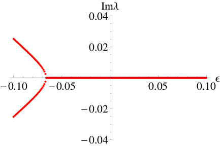
The fixed point FP2 is real in a neighborhood of D=4D=4, however, for ϵ<−0.0663\epsilon<-0.0663 it becomes complex. When one follows the evolution of this FP for increasing ϵ\epsilon, one finds that the complex solution branches into two real solutions. The more negative one is FP2, the more positive one is a new FP that we shall call FP3. When we consider the equation d​λd​τ¯=0\frac{d\lambda}{d\bar{\tau}}=0, we find that all terms are linear in λ\lambda except for the first term in the square bracket, which is independent of λ\lambda. Therefore, λ=0\lambda=0 is not a solution of d​λd​τ¯=0\frac{d\lambda}{d\bar{\tau}}=0. There is however a nontrivial solution which can be found numerically by using the FP values of ω\omega and θ\theta. The values of these FPs as functions of ϵ\epsilon are shown in Fig. 3.

Refer to captionRefer to caption
Figure 3: The real and imaginary parts of ω∗\omega_{*} (top), θ∗\theta_{*} (middle) and λ∗\lambda_{*} (bottom) as functions of ϵ\epsilon. Gray curves: FP2, black curves: FP3.

The analysis of the linearized flow near the FPs shows that λ\lambda is always an UV–attractive eigendirection. For ϵ>0\epsilon>0, both FP2 and FP3 are UV–attractive. (This can happen because they are separated by a repulsive singular line.) For ϵ<0\epsilon<0, FP2 is attractive and FP3 is mixed, with a relevant direction lying mostly in the λ\lambda-θ\theta plane and an irrelevant direction lying mostly in the λ\lambda-ω\omega plane. A picture of the flow in the ω\omega-θ\theta plane is shown in Fig. 4.

Refer to captionRefer to caption
Figure 4: The flow in the ω\omega-θ\theta plane for ϵ=−0.05\epsilon=-0.05 (left) and ϵ=0.05\epsilon=0.05 (right). In both cases the line ω=0\omega=0 is a singularity of the beta functions. Both FPs are UV-attractive for ϵ>0\epsilon>0; FP2 is UV attractive and FP3 is mixed for ϵ<0\epsilon<0.

The most interesting result of this analysis is that FP3 has a natural continuation at D=4D=4 where

FP3:(λ∗,ω∗,θ∗)=(0,0,0.325296).\mbox{FP}_{3}:(\lambda_{*},\omega_{*},\theta_{*})=(0,0,0.325296)\ .

This FP cannot be seen when one directly solves the equations in D=4D=4. The reason is that (in the absence of lower derivative terms, that do not affect the evolution of the four–derivative terms anyway) ω=0\omega=0 corresponds to a Weyl–invariant four–derivative sector. Quantization of this theory requires that also Weyl–invariance be gauge fixed and gives rise to different beta functions from the ones discussed in the preceding section. When one continues to D≠4D\not=4, the theory is no longer Weyl–invariant and the general quantization scheme discussed in this paper is valid. This is a strong indication for the existence of a Weyl–invariant FP in four dimensions. We plan to study this case separately in the future.

7 Three dimensions

Using that in three dimensions R¯μ​ν​ρ​σ2=4​R¯μ​ν2−R¯2\bar{R}_{\mu\nu\rho\sigma}^{2}=4\bar{R}_{\mu\nu}^{2}-\bar{R}^{2}, γ\gamma automatically disappears from the expressions of the beta functions when one makes the replacement α→α−γ,β→β−4​γ\alpha\to\alpha-\gamma,\beta\to\beta-4\gamma. We then obtain for α~=k​α\tilde{\alpha}=k\alpha and β~=k​β\tilde{\beta}=k\beta:

βα~\displaystyle\beta_{\tilde{\alpha}}\hskip-5.69054pt =\displaystyle= α~−1960​π2[(1+47​α~β~+64​α~2β~2−128​α~2​α~+β~)−2​β~α~\displaystyle\hskip-5.69054pt\tilde{\alpha}-\frac{1}{960\pi^{2}}\Bigg[\left(1+\frac{47\tilde{\alpha}}{\tilde{\beta}}+\frac{64\tilde{\alpha}^{2}}{\tilde{\beta}^{2}}-\frac{128\tilde{\alpha}}{2\tilde{\alpha}+\tilde{\beta}}\right)\sqrt{-\frac{2\tilde{\beta}}{\tilde{\alpha}}} (7.1)
+8(129+46​α~β~−114​α~2β~2+32​α~2​α~+β~+α~131​α~+49​β~(8​α~+3​β~)2)],\displaystyle+8\Bigg(129+\frac{46\tilde{\alpha}}{\tilde{\beta}}-\frac{114\tilde{\alpha}^{2}}{\tilde{\beta}^{2}}+\frac{32\tilde{\alpha}}{2\tilde{\alpha}+\tilde{\beta}}+\tilde{\alpha}\frac{131\tilde{\alpha}+49\tilde{\beta}}{(8\tilde{\alpha}+3\tilde{\beta})^{2}}\Bigg)\Bigg],
ββ~\displaystyle\beta_{\tilde{\beta}}\hskip-5.69054pt =\displaystyle= β~+11440​π2[−3(1−113​α~β~+64​α~2β~2+192​α~2​α~+β~)−2​β~α~\displaystyle\hskip-5.69054pt\tilde{\beta}+\frac{1}{1440\pi^{2}}\Bigg[-3\left(1-\frac{113\tilde{\alpha}}{\tilde{\beta}}+\frac{64\tilde{\alpha}^{2}}{\tilde{\beta}^{2}}+\frac{192\tilde{\alpha}}{2\tilde{\alpha}+\tilde{\beta}}\right)\sqrt{-\frac{2\tilde{\beta}}{\tilde{\alpha}}} (7.2)
+8(413−93​α~β~+72​α~2β~2+144​α~2​α~+β~+α~652​α~+243​β~(8​α~+3​β~)2)].\displaystyle+8\Bigg(413-\frac{93\tilde{\alpha}}{\tilde{\beta}}+\frac{72\tilde{\alpha}^{2}}{\tilde{\beta}^{2}}+\frac{144\tilde{\alpha}}{2\tilde{\alpha}+\tilde{\beta}}+\tilde{\alpha}\frac{652\tilde{\alpha}+243\tilde{\beta}}{(8\tilde{\alpha}+3\tilde{\beta})^{2}}\Bigg)\Bigg].

These form a closed system of equations with a FP at α~=0.0496\tilde{\alpha}=0.0496, β~=−0.1381\tilde{\beta}=-0.1381.

The beta functions of Λ~≡Λ/k2\tilde{\Lambda}\equiv\Lambda/k^{2} and G~≡G​k\tilde{G}\equiv G\,k are

βΛ~\displaystyle\beta_{\tilde{\Lambda}} =\displaystyle= −2​Λ~+p⁡(α~,β~)​Λ~−q⁡(α~,β~)​G~​Λ~+r⁡(α~,β~)​G~+s⁡(α~,β~)+t⁡(α~,β~)G~,\displaystyle-2\tilde{\Lambda}+p(\tilde{\alpha},\tilde{\beta})\tilde{\Lambda}-q(\tilde{\alpha},\tilde{\beta})\tilde{G}\tilde{\Lambda}+r(\tilde{\alpha},\tilde{\beta})\tilde{G}+s(\tilde{\alpha},\tilde{\beta})+\frac{t(\tilde{\alpha},\tilde{\beta})}{\tilde{G}}\ , (7.3)
βG~\displaystyle\beta_{\tilde{G}} =\displaystyle= G~−u⁡(α~,β~)​G~−q⁡(α~,β~)​G~2,\displaystyle\tilde{G}-u(\tilde{\alpha},\tilde{\beta})\tilde{G}-q(\tilde{\alpha},\tilde{\beta})\tilde{G}^{2}\ , (7.4)

where

p⁡(α~,β~)\displaystyle p(\tilde{\alpha},\tilde{\beta})\hskip-5.69054pt =\displaystyle= −2304​α~3+1120​α~2​β~+1778​α~​β~2+387​β~348​π2​(8​α~+3​β~)2​β~2,\displaystyle\hskip-5.69054pt\frac{-2304\tilde{\alpha}^{3}+1120\tilde{\alpha}^{2}\tilde{\beta}+1778\tilde{\alpha}\tilde{\beta}^{2}+387\tilde{\beta}^{3}}{48\pi^{2}(8\tilde{\alpha}+3\tilde{\beta})^{2}\tilde{\beta}^{2}}, (7.5)
q⁡(α~,β~)\displaystyle q(\tilde{\alpha},\tilde{\beta})\hskip-5.69054pt =\displaystyle= 13​π​σ​[37+β~8​α~+3​β~−16​α~β~+−2​β~α~+4​(1−8​α~β~)​−2​α~β~],\displaystyle\hskip-5.69054pt\frac{1}{3\pi\sigma}\left[37+\frac{\tilde{\beta}}{8\tilde{\alpha}+3\tilde{\beta}}-\frac{16\tilde{\alpha}}{\tilde{\beta}}+\sqrt{-\frac{2\tilde{\beta}}{\tilde{\alpha}}}+4\left(1-\frac{8\tilde{\alpha}}{\tilde{\beta}}\right)\sqrt{\frac{-2\tilde{\alpha}}{\tilde{\beta}}}\right],~~~~ (7.6)
r⁡(α~,β~)\displaystyle r(\tilde{\alpha},\tilde{\beta})\hskip-5.69054pt =\displaystyle= 13​π2​[24−12​(−2​β~α~)3/2−8​(−2​α~β~)3/2],\displaystyle\hskip-5.69054pt\frac{1}{3\pi^{2}}\left[24-\frac{1}{2}\left(\frac{-2\tilde{\beta}}{\tilde{\alpha}}\right)^{3/2}-8\left(\frac{-2\tilde{\alpha}}{\tilde{\beta}}\right)^{3/2}\right], (7.7)
s⁡(α~,β~)\displaystyle s(\tilde{\alpha},\tilde{\beta})\hskip-5.69054pt =\displaystyle= −σ​16​α~+5​β~8​π2​(8​α~+3​β~)​β~,\displaystyle\hskip-5.69054pt-\sigma\frac{16\tilde{\alpha}+5\tilde{\beta}}{8\pi^{2}(8\tilde{\alpha}+3\tilde{\beta})\tilde{\beta}}, (7.8)
t⁡(α~,β~)\displaystyle t(\tilde{\alpha},\tilde{\beta})\hskip-5.69054pt =\displaystyle= 3​σ2​128​α~2+96​α~​β~+19​β~21024​π3​(8​α~+3​β~)2​β~2,\displaystyle\hskip-5.69054pt3\sigma^{2}\frac{128\tilde{\alpha}^{2}+96\tilde{\alpha}\tilde{\beta}+19\tilde{\beta}^{2}}{1024\pi^{3}(8\tilde{\alpha}+3\tilde{\beta})^{2}\tilde{\beta}^{2}}, (7.9)
u⁡(α~,β~)\displaystyle u(\tilde{\alpha},\tilde{\beta})\hskip-5.69054pt =\displaystyle= 2304​α~3+2912​α~2​β~+1174​α~​β~2+153​β~348​π2​(8​α~+3​β~)2​β~2.\displaystyle\hskip-5.69054pt\frac{2304\tilde{\alpha}^{3}+2912\tilde{\alpha}^{2}\tilde{\beta}+1174\tilde{\alpha}\tilde{\beta}^{2}+153\tilde{\beta}^{3}}{48\pi^{2}(8\tilde{\alpha}+3\tilde{\beta})^{2}\tilde{\beta}^{2}}. (7.10)

If we choose α~\tilde{\alpha} and β~\tilde{\beta} at their FP, one finds a FP at Λ~=0.5355​σ\tilde{\Lambda}=0.5355\sigma and G~=0.1758​σ\tilde{G}=0.1758\sigma, with eigenvalues −2.866-2.866 and −1.235-1.235. Thus this is a UV–stable FP. This flow is depicted in Fig. 5.

Refer to caption
Figure 5: The flow in the (Λ~,G~)(\tilde{\Lambda},\tilde{G})–plane when α~\tilde{\alpha} and β~\tilde{\beta} are at FP1

Note that there is no Gaussian FP in this plane because α~\tilde{\alpha} and β~\tilde{\beta} are already at a nontrivial FP.

Let us change coordinates and consider the beta functions of the couplings λ3=1/β\lambda_{3}=1/\beta and ω3=−2α/β\omega_{3}=-2\alpha/\beta. These coupling constants are similar but different from those defined in the action (2.4). We find that they are given by

βλ3\displaystyle\beta_{\lambda_{3}}\hskip-5.69054pt =\displaystyle= −λ3−λ32480​π2​ω3​(ω3−1)[2−81ω3−81ω32−32ω33\displaystyle\hskip-5.69054pt-\lambda_{3}-\frac{\lambda_{3}^{2}}{480\pi^{2}\sqrt{\omega_{3}}(\omega_{3}-1)}\Big[2-81\omega_{3}-81\omega_{3}^{2}-32\omega_{3}^{3} (7.11)
+8​ω3​(−1239+4660​ω3−5720​ω32+2219​ω33+8​ω34+96​ω35)(4​ω3−3)2],\displaystyle\hskip-5.69054pt+\frac{8\sqrt{\omega_{3}}(-1239+4660\omega_{3}-5720\omega_{3}^{2}+2219\omega_{3}^{3}+8\omega_{3}^{4}+96\omega_{3}^{5})}{(4\omega_{3}-3)^{2}}\Big],
βω3\displaystyle\beta_{\omega_{3}}\hskip-5.69054pt =\displaystyle= −λ3480​π2​ω3​(ω3−1)[(1+ω3)(2+79ω3−81ω32−32ω33)\displaystyle\hskip-5.69054pt-\frac{\lambda_{3}}{480\pi^{2}\sqrt{\omega_{3}}(\omega_{3}-1)}\Big[(1+\omega_{3})(2+79\omega_{3}-81\omega_{3}^{2}-32\omega_{3}^{3}) (7.12)
+2​ω3​(4644−23486​ω3+43055​ω32−32209​ω33+5788​ω34+1856​ω35+384​ω36)(4​ω3−3)2].\displaystyle\hskip-5.69054pt+\frac{2\sqrt{\omega_{3}}(4644-23486\omega_{3}+43055\omega_{3}^{2}-32209\omega_{3}^{3}+5788\omega_{3}^{4}+1856\omega_{3}^{5}+384\omega_{3}^{6})}{(4\omega_{3}-3)^{2}}\Big].~~

We see that the beta functions vanish for λ3=0\lambda_{3}=0, leaving ω3\omega_{3} undetermined. In this variable, we see that we can have the Gaussian FP for λ3=0\lambda_{3}=0 with fixed ω3\omega_{3}, corresponding to β~→∞\tilde{\beta}\to\infty with α~/β~\tilde{\alpha}/\tilde{\beta} = fixed and s=t=0s=t=0. As in four dimensions, using the variable τ¯\bar{\tau} defined by d​τ¯=λ3​d​k/kd\bar{\tau}=\lambda_{3}dk/k removes one power of λ3\lambda_{3} from the beta functions and one finds a FP at (λ3,ω3)=(−7.240,0.7187)(\lambda_{3},\omega_{3})=(-7.240,0.7187). Another important result is that 8​α~+3​β~8\tilde{\alpha}+3\tilde{\beta} does not vanish at the FP. This implies that the new massive gravity does not correspond to the FP. This was suggested in [29], and we confirm it.

8 Five dimensions

In dimensions D≠4D\not=4, ω\omega and θ\theta remain dimensionless but λ\lambda has dimension 4−D4-D, so we define λ~=λ​kD−4\tilde{\lambda}=\lambda\,k^{D-4}. We find the following beta functions:

βλ~\displaystyle\beta_{\tilde{\lambda}} =\displaystyle= λ~+λ~23360​(4​π)3​ω2​(ω−1)[−60(ω−1)(621ω2−42ω+1)θ2\displaystyle\tilde{\lambda}+\frac{\tilde{\lambda}^{2}}{3360(4\pi)^{3}\omega^{2}(\omega-1)}\Big[-60(\omega-1)(621\omega^{2}-42\omega+1)\theta^{2} (8.1)
+80​(279​ω−2)​(ω−1)​ω​θ−(270​ω4+1290​ω3+131258​ω2−112798​ω+460)​ω\displaystyle+80(279\omega-2)(\omega-1)\omega\theta-(270\omega^{4}+1290\omega^{3}+131258\omega^{2}-112798\omega+460)\omega
+2ω2243​ω4+1872​ω3+8922​ω2+18304​ω+116193​ω+5],\displaystyle+\sqrt{2}\omega^{2}\frac{243\omega^{4}+1872\omega^{3}+8922\omega^{2}+18304\omega+11619}{\sqrt{3\omega+5}}\Big],
βω\displaystyle\beta_{\omega} =\displaystyle= λ~3360​(4​π)3​(ω−1)​ω2[60(1−ω)(621ω3+147ω2−17ω+9)θ2\displaystyle\frac{\tilde{\lambda}}{3360(4\pi)^{3}(\omega-1)\omega^{2}}\Big[60(1-\omega)(621\omega^{3}+147\omega^{2}-17\omega+9)\theta^{2}
+40​(1−ω)​(9​ω2−446​ω−63)​ω​θ\displaystyle+40(1-\omega)(9\omega^{2}-446\omega-63)\omega\theta
−(270​ω4+30810​ω3+130058​ω2−124370​ω−4000)​ω2\displaystyle-(270\omega^{4}+30810\omega^{3}+130058\omega^{2}-124370\omega-4000)\omega^{2}
+2ω2243​ω5+2925​ω4+15690​ω3+32326​ω2+20003​ω−56513​ω+5],\displaystyle+\sqrt{2}\omega^{2}\frac{243\omega^{5}+2925\omega^{4}+15690\omega^{3}+32326\omega^{2}+20003\omega-5651}{\sqrt{3\omega+5}}\Big],
βθ\displaystyle\beta_{\theta} =\displaystyle= λ~20160​(4​π)3​(ω−1)​ω2[−360(ω−1)(621ω2−42ω+1)θ3\displaystyle\frac{\tilde{\lambda}}{20160(4\pi)^{3}(\omega-1)\omega^{2}}\Big[-360(\omega-1)(621\omega^{2}-42\omega+1)\theta^{3} (8.2)
−12​(135​ω4+645​ω3+70189​ω2−60679​ω−50)​θ​ω\displaystyle-12(135\omega^{4}+645\omega^{3}+70189\omega^{2}-60679\omega-50)\theta\omega
+60​(ω−1)​(2799​ω2−106​ω+3)​θ2+10​(81​ω3+387​ω2+23103​ω−17427)​ω2\displaystyle+60(\omega-1)(2799\omega^{2}-106\omega+3)\theta^{2}+10(81\omega^{3}+387\omega^{2}+23103\omega-17427)\omega^{2}
+6​23​ω+5​(243​ω4+1872​ω3+8922​ω2+18304​ω+11619)​θ​ω2\displaystyle+6\sqrt{\frac{2}{3\omega+5}}\Big(243\omega^{4}+1872\omega^{3}+8922\omega^{2}+18304\omega+11619\Big)\theta\omega^{2}
−323​ω+5(243ω4+1872ω3+8698ω2+17856ω+12291)ω2].\displaystyle-3\sqrt{\frac{2}{3\omega+5}}(243\omega^{4}+1872\omega^{3}+8698\omega^{2}+17856\omega+12291)\omega^{2}\Big].

In the standard RG time t=log⁡kt=\log k, these beta functions have a FP for λ~=0\tilde{\lambda}=0 and undetermined values of ω\omega and θ\theta. The flow in this sector is therefore studied more conveniently using the variable τ¯\bar{\tau}, which has the effect of removing one power of λ~\tilde{\lambda} from the beta functions. There is then no FP with λ~=0\tilde{\lambda}=0 but there are four FPs with coordinates given in the following table:

λ~∗\tilde{\lambda}_{*} ω∗\omega_{*} θ∗\theta_{*}
FP1 1.26541.2654 1007.91007.9 −406.9-406.9
FP2 −0.61121-0.61121 1796.01796.0 841.4841.4
FP3 −9.4483-9.4483 27.927.9 0.540.54
FP4 53.5353.53 −0.082-0.082 0.270.27

For Λ~\tilde{\Lambda} and G~\tilde{G} we have the beta functions:

βΛ~\displaystyle\beta_{\tilde{\Lambda}} =\displaystyle= −2​Λ~−λ~​σ​(9​ω+1)64​π3​ω+15​λ~2​σ2​(9​ω2+1)32768​π4​G~​ω2+Λ~​[6​(9​ω2+1)​θ+ω⁡(135​ω2+280​ω+3)]1024​π3​ω2​λ~\displaystyle-2\tilde{\Lambda}-\frac{\tilde{\lambda}\sigma(9\omega+1)}{64\pi^{3}\omega}+\frac{15\tilde{\lambda}^{2}\sigma^{2}(9\omega^{2}+1)}{32768\pi^{4}\tilde{G}\omega^{2}}+\frac{\tilde{\Lambda}\Big[6(9\omega^{2}+1)\theta+\omega(135\omega^{2}+280\omega+3)\Big]}{1024\pi^{3}\omega^{2}}\tilde{\lambda} (8.3)
−G~2​(3​ω+5)5−2304​(3​ω+5)5/2+16384​2960​π2​(3​ω+5)5/2−G~​Λ~1440​π2​σ​ω[144θ(9ω+1)\displaystyle-\tilde{G}\frac{\sqrt{2}(3\omega+5)^{5}-2304(3\omega+5)^{5/2}+16384\sqrt{2}}{960\pi^{2}(3\omega+5)^{5/2}}-\frac{\tilde{G}\tilde{\Lambda}}{1440\pi^{2}\sigma\omega}\Big[144\theta(9\omega+1)
+(2952ω+3240)ω+23​ω+5(81ω3+495ω2+975ω+625)ω+2560​2​ω(3​ω+5)3/2],\displaystyle+(2952\omega+3240)\omega+\sqrt{\frac{2}{3\omega+5}}(81\omega^{3}+495\omega^{2}+975\omega+625)\omega+\frac{2560\sqrt{2}\omega}{(3\omega+5)^{3/2}}\Big],~~~~
βG~\displaystyle\beta_{\tilde{G}} =\displaystyle= 3G~+G~1024​π3​ω2(6θ(9ω2+1)+ω(135ω2−180ω−17))λ~−G~21440​π2​σ​ω[144θ(9ω+1)\displaystyle 3\tilde{G}+\frac{\tilde{G}}{1024\pi^{3}\omega^{2}}\Big(6\theta(9\omega^{2}+1)+\omega(135\omega^{2}-180\omega-17)\Big)\tilde{\lambda}-\frac{\tilde{G}^{2}}{1440\pi^{2}\sigma\omega}\Big[144\theta(9\omega+1) (8.4)
+ω(2952ω+3240)+23​ω+5(81ω3+495ω2+975ω+625)ω+2560​2​ω(3​ω+5)3/2].\displaystyle+\omega(2952\omega+3240)+\sqrt{\frac{2}{3\omega+5}}(81\omega^{3}+495\omega^{2}+975\omega+625)\omega+\frac{2560\sqrt{2}\omega}{(3\omega+5)^{3/2}}\Big].

The Gaussian FP corresponds to λ~=G~=Λ~=0\tilde{\lambda}=\tilde{G}=\tilde{\Lambda}=0, with arbitrary values of ω\omega and θ\theta. One finds that the eigenvalues of the linearized flow equation at this point are equal to 33, −2-2, 11, 00, 00, which are just the opposites of the canonical dimensions of GG, Λ\Lambda, λ\lambda, ω\omega and θ\theta, as expected.

Next we consider FPs with λ~∗≠0\tilde{\lambda}_{*}\not=0. We take the FP values of λ~\tilde{\lambda}, ω\omega and θ\theta given in the table above and use them in the beta functions of G~\tilde{G}, Λ~\tilde{\Lambda}. One finds various FPs with G~\tilde{G} and Λ~\tilde{\Lambda} either zero or nonzero. If one chooses G~\tilde{G} and Λ~\tilde{\Lambda} equal to zero, the matrix of the derivatives of the beta functions has singularities in some off-diagonal elements (more precisely the derivatives of Λ~\tilde{\Lambda} with respect to λ~\tilde{\lambda}, ω\omega and G~\tilde{G}). We will not consider this case further. The FPs with non-zero Λ~\tilde{\Lambda} and G~\tilde{G} are

G~∗\tilde{G}_{*} Λ~∗\tilde{\Lambda}_{*}
FP1 4.992×10−54.992\times 10^{-5} −0.4839-0.4839
FP2 −3.976×10⁻⁶-3.976\times 10^{-6} −0.5397-0.5397
FP3 6.619×10−26.619\times 10^{-2} −0.1201-0.1201
FP4 13.7413.74 0.60380.6038

(These are the values for σ=1\sigma=1; for σ=−1\sigma=-1 all the elements of the table have opposite sign.)

Of these FPs, the second and the third are physically uninteresting because of the sign of λ~∗\tilde{\lambda}_{*}. The first three also have suspiciously small values for G~\tilde{G} and the first two also have one very large critical exponent (of order 10310^{3}). It is possible that these are spurious FPs of the type that often appear in polynomial truncations. The fourth is more promising: the values of G~\tilde{G} and Λ~\tilde{\Lambda} are closer to those found in the Einstein-Hilbert truncation. The critical exponents at this FP are as follows: the cosmological constant is an eigendirection with eigenvalue −4.635-4.635; the remaining eigenvalues are −3.460-3.460 in the direction of G~\tilde{G}, with a small mixture of Λ~\tilde{\Lambda}; −3.150-3.150 in the direction of G~\tilde{G}, with a small mixture of all the other operators; −1-1 in the direction of λ~\tilde{\lambda} with a small mixture of Λ~\tilde{\Lambda} and G~\tilde{G}; −0.9870-0.9870 in the direction of λ~\tilde{\lambda} with small mixtures of all the other operators. This FP is therefore UV attractive in all five directions considered.

9 Six Dimensions

In dimension D=6D=6, we have

βλ~\displaystyle\beta_{\tilde{\lambda}} =\displaystyle= 2λ~+λ~2243×103​(4​π)3​ω2[−1215θ2(24ω−1)(32ω−3)+2700θω(212ω−3)\displaystyle 2\tilde{\lambda}+\frac{\tilde{\lambda}^{2}}{243\times 10^{3}(4\pi)^{3}\omega^{2}}\Big[-1215\theta^{2}(24\omega-1)(32\omega-3)+2700\theta\omega(212\omega-3) (9.1)
+ω4​ω+9(2048ω5+20352ω4+181728ω3−7130808ω2−16720182ω+54675)],\displaystyle+\frac{\omega}{4\omega+9}(2048\omega^{5}+20352\omega^{4}+181728\omega^{3}-7130808\omega^{2}-16720182\omega+54675)\Big],
βω\displaystyle\beta_{\omega} =\displaystyle= −λ~243×103​(4​π)3​ω2[3645θ2(ω+1){16ω(16ω−3)+21}+2700θω{ω(124ω−387)−36}\displaystyle-\frac{\tilde{\lambda}}{243\times 10^{3}(4\pi)^{3}\omega^{2}}\Big[3645\theta^{2}(\omega+1)\{16\omega(16\omega-3)+21\}+2700\theta\omega\{\omega(124\omega-387)-36\} (9.2)
−ω24​ω+9(2048ω5+32640ω4−1510560ω3−10360440ω2−15408630ω+7533)],\displaystyle-\frac{\omega^{2}}{4\omega+9}(2048\omega^{5}+32640\omega^{4}-1510560\omega^{3}-10360440\omega^{2}-15408630\omega+7533)\Big],
βθ\displaystyle\beta_{\theta} =\displaystyle= λ~486×103​(4​π)3​ω2[−2430θ3(24ω−1)(32ω−3)+135θ2{4ω(2918ω−219)+27}\displaystyle\frac{\tilde{\lambda}}{486\times 10^{3}(4\pi)^{3}\omega^{2}}\Big[-2430\theta^{3}(24\omega-1)(32\omega-3)+135\theta^{2}\{4\omega(2918\omega-219)+27\} (9.3)
−32​ω2​(16​ω3+123​ω2+1098​ω−28134)\displaystyle-32\omega^{2}(16\omega^{3}+123\omega^{2}+1098\omega-28134)
+2​θ​ω4​ω+9(2048ω5+20352ω4+181728ω3−7919208ω2−18526482ω−18225)].\displaystyle+\frac{2\theta\omega}{4\omega+9}(2048\omega^{5}+20352\omega^{4}+181728\omega^{3}-7919208\omega^{2}-18526482\omega-18225)\Big].

Proceeding as in the five–dimensional cases one finds seven FPs:

λ~∗\tilde{\lambda}_{*} ω∗\omega_{*} θ∗\theta_{*}
FP1 148.358148.358 105.0105.0 −25.98-25.98
FP2 −37.24-37.24 265.4265.4 103.0103.0
FP3 55.5455.54 −33.17-33.17 0.47010.4701
FP4 −106.647-106.647 24.5824.58 0.55440.5544
FP5 502.2502.2 −4.545-4.545 0.24930.2493
FP6 396.5396.5 −2.268-2.268 0.18710.1871
FP7 513.725513.725 −0.1376-0.1376 0.24480.2448

Upon substituting these values in the beta functions for Λ~\tilde{\Lambda} and G~\tilde{G}.

βΛ~\displaystyle\beta_{\tilde{\Lambda}}\hskip-5.69054pt =\displaystyle= −2​Λ~−λ~​σ​(28​ω+3)768​π3​ω+λ~2​σ2​(56​ω2+9)49152​π4​G~​ω2+Λ~​[3​(56​ω2+9)​θ+(168​ω2+286​ω+3)​ω]5760​π3​ω2​λ~\displaystyle\hskip-5.69054pt-2\tilde{\Lambda}-\frac{\tilde{\lambda}\sigma(28\omega+3)}{768\pi^{3}\omega}+\frac{\tilde{\lambda}^{2}\sigma^{2}(56\omega^{2}+9)}{49152\pi^{4}\tilde{G}\omega^{2}}+\frac{\tilde{\Lambda}\Big[3(56\omega^{2}+9)\theta+(168\omega^{2}+286\omega+3)\omega\Big]}{5760\pi^{3}\omega^{2}}\tilde{\lambda} (9.4)
+G~π2[916−112516​(4​ω+9)3−(4​ω+9)381000]−G~​Λ~81000​π2​σ​ω[1350θ(28ω+3)\displaystyle+\frac{\tilde{G}}{\pi^{2}}\Big[\frac{9}{16}-\frac{1125}{16(4\omega+9)^{3}}-\frac{(4\omega+9)^{3}}{81000}\Big]-\frac{\tilde{G}\tilde{\Lambda}}{81000\pi^{2}\sigma\omega}\Big[1350\theta(28\omega+3)
+ω(4​ω+9)2(2048ω5+26880ω4+714240ω3+3346920ω2+5175900ω+2646513)],\displaystyle+\frac{\omega}{(4\omega+9)^{2}}(2048\omega^{5}+26880\omega^{4}+714240\omega^{3}+3346920\omega^{2}+5175900\omega+2646513)\Big],~~~~~~
βG~\displaystyle\beta_{\tilde{G}}\hskip-5.69054pt =\displaystyle= 4G~+G~5760​π3​ω2[3θ(56ω2+9)+2ω(84ω2−163ω−12)]λ~−G~281000​π2​σ​ω[1350θ(28ω+3)\displaystyle\hskip-5.69054pt4\tilde{G}+\frac{\tilde{G}}{5760\pi^{3}\omega^{2}}\Big[3\theta(56\omega^{2}+9)+2\omega(84\omega^{2}-163\omega-12)\Big]\tilde{\lambda}-\frac{\tilde{G}^{2}}{81000\pi^{2}\sigma\omega}\Big[1350\theta(28\omega+3) (9.5)
+ω(4​ω+9)2(2048ω5+26880ω4+714240ω3+3346920ω2+5175900ω+2646513)].\displaystyle+\frac{\omega}{(4\omega+9)^{2}}(2048\omega^{5}+26880\omega^{4}+714240\omega^{3}+3346920\omega^{2}+5175900\omega+2646513)\Big].

one finds the following values of G~∗\tilde{G}_{*} and Λ~∗\tilde{\Lambda}_{*}:

G~∗\tilde{G}_{*} Λ~∗\tilde{\Lambda}_{*}
FP1 0.07220030.0722003 −0.679014-0.679014
FP2 −0.00284264-0.00284264 −0.211878-0.211878
FP3 −0.372332-0.372332 −0.183136-0.183136
FP4 0.3744080.374408 −0.0119273-0.0119273
FP5 −6.84831-6.84831 −0.342368-0.342368
FP6 0.02695670.0269567 129.099129.099
FP7 123.127123.127 1.160441.16044

(These are the values for σ=1\sigma=1; for σ=−1\sigma=-1 all the elements of the table have opposite sign.)

Of these fixed points, FP3, FP4, FP6 and FP7 are UV attractive in all directions; the others have one or two irrelevant directions.

10 Conclusions

We have studied the one-loop beta functions in higher derivative gravity for general background in arbitrary dimensions. The results for D=4D=4 agree with the literature, up to minor differences due to the scheme–dependence of certain coefficients. In the four–derivative sector, there are at one loop two well–known fixed points FP1 and FP2. To each of these there correspond two FPs in the Λ~\tilde{\Lambda}–G~\tilde{G} planes. There is a Gaussian FP, which is UV–attractive in the Λ~\tilde{\Lambda} direction and repulsive along a complementary direction, making G~\tilde{G} (with a small mixture of Λ~\tilde{\Lambda}) an irrelevant coupling. There is also a non-Gaussian FP that is UV–attractive in both directions. Altogether the qualitative structure of the flow in the Λ~\tilde{\Lambda}–G~\tilde{G} planes is surprisingly similar to that of the theory in the Einstein–Hilbert truncation. The main difference is the reality of the critical exponents, to be contrasted with the complex conjugate critical exponents seen in the Einstein–Hilbert truncation of the flow, which lead to spiralling trajectories near the non-Gaussian FP. It may be that the approximation used here is too crude. On the other hand, recent studies of the Einstein–Hilbert truncation taking into account the anomalous dimension of the fluctuation field hμ​νh_{\mu\nu} find real critical exponents in that case too [35, 36]. (See also the general argument in [37].) To settle the question of the correct critical exponents, one may have to perform more complicated calculations, for example the full truncated RG of higher derivative gravity taking into account the anomalous dimension of the fluctuation field. Another issue that could be clarified by such a calculation is the position of the FP of the dimensionless coupling λ~\tilde{\lambda}, which was found to occur at some non-zero value in [15].

In this paper we have extended the calculation of one-loop beta functions of higher derivative gravity to arbitrary dimension. Insofar as the beta functions can be obtained directly as finite quantities, without having to refer to divergences and regulators, the dimension can be treated formally as a continuous parameter of the theory. In this way the structure of the FPs can be reliably studied as a function of dimension. There has been one previous study along these lines [9], but our results differ significantly. This can be traced to the structure of the heat kernel coefficients of fourth–order and of non–minimal second order operators, that we have taken from [33, 34]. We find that FP1 becomes complex as soon as one departs from D=4D=4, but FP2 remains real in a neighborhood of D=4D=4. Furthermore, for arbitrarily small ϵ\epsilon, there is another fixed point FP3 which does not solve our beta functions in D=4D=4. We believe that this FP must correspond to a Weyl–invariant theory, which requires a different quantization procedure. We hope to return on this point in the future.

One of the main motivations of this work was the structure of higher derivative gravity in D=3D=3. Due to the fact that in D=3D=3, E=0E=0 identically, there are only two independent beta functions in the four–derivative sector, and the FP structure is different from D=4D=4. In fact, when D≲3.93D\lesssim 3.93 the fixed points FP2 and FP3 merge and become complex. Nevertheless, there is also in D=3D=3 a non-Gaussian FP with non–vanishing values of α~\tilde{\alpha} and β~\tilde{\beta} (recall that the four–derivative couplings are dimensionful in D=3D=3). The corresponding flow in the Λ~\tilde{\Lambda}–G~\tilde{G} planes has a non–Gaussian FP that is somewhat similar to the one that is found in the Einstein–Hilbert truncation or in the Chern–Simons theory, except that it has a relatively large value of Λ~\tilde{\Lambda}. An important point is that new massive gravity does not correspond to a FP, confirming the result in [29].

On the other hand, when one goes to dimensions greater than four the fixed points FP2 and FP3 remain real but there appear further FPs. There is always a Gaussian FP with λ~=Λ~=G~=0\tilde{\lambda}=\tilde{\Lambda}=\tilde{G}=0 and unspecified ω\omega and θ\theta, but there are also FPs with λ~≠0\tilde{\lambda}\not=0. It is difficult, within the present analysis, to establish which ones of these are physical and which ones are mere truncation artifacts.

Acknowledgment

We would like to thank Ilya Shapiro for valuable discussions. Part of this work was carried out while the authors were attending the workshops “Topics in Holography, Supersymmetry and Higher Derivatives” at Texas A&M University, and “2nd Mediterranean Conference on Classical and Quantum Gravity” at Veli Lošinj, Croatia. We thank the organizers for invitation and providing stimulating atmosphere. This work was supported in part by the Grant-in-Aid for Scientific Research Fund of the JSPS (C) No. 24540290, and (A) No. 22244030.

Appendix A Conventions and useful formulae

Here we summarize our conventions and formulae necessary in the text. We give these such that they are valid for any dimension DD.

Our signature of the metric is (−,+,…+)(-,+,\dots+) and the curvature tensors are given as

Rαβ​μ​ν\displaystyle R^{\alpha}{}_{\beta\mu\nu} =\displaystyle= ∂μΓβ​να−∂νΓβ​μα+Γμ​λα​Γβ​νλ−Γν​λα​Γβ​μλ,\displaystyle\partial_{\mu}\Gamma^{\alpha}_{\beta\nu}-\partial_{\nu}\Gamma^{\alpha}_{\beta\mu}+\Gamma^{\alpha}_{\mu\lambda}\Gamma^{\lambda}_{\beta\nu}-\Gamma^{\alpha}_{\nu\lambda}\Gamma^{\lambda}_{\beta\mu},
Rμ​ν\displaystyle R_{\mu\nu} =\displaystyle= Rαμ​α​ν.\displaystyle R^{\alpha}{}_{\mu\alpha\nu}. (A.1)

The backgrounds are denoted with overbar. Expansion around the background gives

Γμ​να\displaystyle\Gamma^{\alpha}_{\mu\nu} =\displaystyle= Γ¯μ​να+Γμ​να⁡(1)+Γμ​να⁡(2),\displaystyle\bar{\Gamma}^{\alpha}_{\mu\nu}+\Gamma^{\alpha(1)}_{\mu\nu}+\Gamma^{\alpha(2)}_{\mu\nu}, (A.2)

where

Γμ​να⁡(1)\displaystyle\Gamma^{\alpha(1)}_{\mu\nu} =\displaystyle= 12(∇νhα+μ∇μhα−ν∇αhμ​ν),\displaystyle\frac{1}{2}(\nabla_{\nu}h^{\alpha}{}_{\mu}+\nabla_{\mu}h^{\alpha}{}_{\nu}-\nabla^{\alpha}h_{\mu\nu}), (A.3)
Γμ​να⁡(2)\displaystyle\Gamma^{\alpha(2)}_{\mu\nu} =\displaystyle= −12​hα​β​(∇νhμ​β+∇μhν​β−∇βhμ​ν).\displaystyle-\frac{1}{2}h^{\alpha\beta}(\nabla_{\nu}h_{\mu\beta}+\nabla_{\mu}h_{\nu\beta}-\nabla_{\beta}h_{\mu\nu}). (A.4)

Note that

−g=−g¯​[1+12​h+18​(h2−2​hμ​ν2)+O⁡(h3)].\displaystyle\sqrt{-g}=\sqrt{-\bar{g}}\Big[1+\frac{1}{2}h+\frac{1}{8}(h^{2}-2h_{\mu\nu}^{2})+O(h^{3})\Big]. (A.5)

We find, to the second order,

Rμν​α​β\displaystyle R^{\mu}{}_{\nu\alpha\beta}\!\! =\displaystyle= R¯μν​α​β+Rμν​α​β(1)+Rμν​α​β(2),\displaystyle\!\!\bar{R}^{\mu}{}_{\nu\alpha\beta}+R^{\mu}{}_{\nu\alpha\beta}^{(1)}+R^{\mu}{}_{\nu\alpha\beta}^{(2)},
Rμν​α​β(1)\displaystyle R^{\mu}{}_{\nu\alpha\beta}^{(1)}\!\! =\displaystyle= 12​(∇α∇ν​hβμ−∇α∇μ​hν​β−∇β∇ν​hαμ+∇β∇μ​hν​α)+12​R¯ν​γ​α​β​hμ​γ+12​R¯μ​hνγγ​α​β,\displaystyle\!\!\frac{1}{2}(\nabla_{\alpha}\nabla_{\nu}h^{\mu}_{\beta}-\nabla_{\alpha}\nabla^{\mu}h_{\nu\beta}-\nabla_{\beta}\nabla_{\nu}h^{\mu}_{\alpha}+\nabla_{\beta}\nabla^{\mu}h_{\nu\alpha})+\frac{1}{2}\bar{R}_{\nu\gamma\alpha\beta}h^{\mu\gamma}+\frac{1}{2}\bar{R}^{\mu}{}_{\gamma\alpha\beta}h^{\gamma}_{\nu},~~~ (A.6)
Rμν​α​β(2)\displaystyle R^{\mu}{}_{\nu\alpha\beta}^{(2)}\!\! =\displaystyle= ∇αΓν​βμ⁡(2)−∇βΓν​αμ⁡(2)+Γλ​αμ⁡(1)​Γν​βλ⁡(1)−Γλ​βμ⁡(1)​Γν​αλ⁡(1)\displaystyle\!\!\nabla_{\alpha}\Gamma^{\mu(2)}_{\nu\beta}-\nabla_{\beta}\Gamma^{\mu(2)}_{\nu\alpha}+\Gamma^{\mu(1)}_{\lambda\alpha}\Gamma^{\lambda(1)}_{\nu\beta}-\Gamma^{\mu(1)}_{\lambda\beta}\Gamma^{\lambda(1)}_{\nu\alpha} (A.7)
=\displaystyle= −12​hμ​γ​∇α(∇βhν​γ+∇νhβ​γ−∇γhν​β)−14​∇αhμ​γ​(∇βhν​γ+∇νhβ​γ−∇γhν​β)\displaystyle\!\!-\frac{1}{2}h^{\mu\gamma}\nabla_{\alpha}(\nabla_{\beta}h_{\nu\gamma}+\nabla_{\nu}h_{\beta\gamma}-\nabla_{\gamma}h_{\nu\beta})-\frac{1}{4}\nabla_{\alpha}h^{\mu\gamma}(\nabla_{\beta}h_{\nu\gamma}+\nabla_{\nu}h_{\beta\gamma}-\nabla_{\gamma}h_{\nu\beta})
+14​∇γhαμ​(∇βhνγ+∇νhβγ−∇γhν​β)−14​∇μhα​γ​(∇βhνγ+∇νhβγ−∇γhν​β)\displaystyle\hskip-5.69054pt+\;\frac{1}{4}\nabla_{\gamma}h^{\mu}_{\alpha}(\nabla_{\beta}h^{\gamma}_{\nu}+\nabla_{\nu}h^{\gamma}_{\beta}-\nabla^{\gamma}h_{\nu\beta})-\frac{1}{4}\nabla^{\mu}h_{\alpha\gamma}(\nabla_{\beta}h^{\gamma}_{\nu}+\nabla_{\nu}h^{\gamma}_{\beta}-\nabla^{\gamma}h_{\nu\beta})
−(α↔β).\displaystyle-(\alpha\leftrightarrow\beta).

Though the last one looks different from that in [8], it coincides. Similarly

Rμ​ν(1)\displaystyle R^{(1)}_{\mu\nu}\!\! =\displaystyle= −12​(∇μ∇ν​h−∇μhν−∇νhμ+□​hμ​ν)−R¯α​μ​β​ν​hα​β+12​R¯μ​α​hνα+12​R¯ν​α​hμα,\displaystyle\!\!-\frac{1}{2}(\nabla_{\mu}\nabla_{\nu}h-\nabla_{\mu}h_{\nu}-\nabla_{\nu}h_{\mu}+\Box h_{\mu\nu})-\bar{R}_{\alpha\mu\beta\nu}h^{\alpha\beta}+\frac{1}{2}\bar{R}_{\mu\alpha}h^{\alpha}_{\nu}+\frac{1}{2}\bar{R}_{\nu\alpha}h^{\alpha}_{\mu},
Rμ​ν(2)\displaystyle R^{(2)}_{\mu\nu}\!\! =\displaystyle= 12​∇μ(hα​β​∇νhα​β)−12​∇α{hα​β​(∇μhν​β+∇νhμ​β−∇βhμ​ν)}\displaystyle\!\!\frac{1}{2}\nabla_{\mu}(h^{\alpha\beta}\nabla_{\nu}h_{\alpha\beta})-\frac{1}{2}\nabla_{\alpha}\{h^{\alpha\beta}(\nabla_{\mu}h_{\nu\beta}+\nabla_{\nu}h_{\mu\beta}-\nabla_{\beta}h_{\mu\nu})\}
−14​(∇μhαβ+∇αhμβ−∇βhα​μ)​(∇βhνα+∇νhβα−∇αhβ​ν)+14​∇αh​(∇μhνα+∇νhμα−∇αhμ​ν),\displaystyle\hskip-28.45274pt-\frac{1}{4}(\nabla_{\mu}h^{\beta}_{\alpha}+\nabla_{\alpha}h^{\beta}_{\mu}-\nabla^{\beta}h_{\alpha\mu})(\nabla_{\beta}h^{\alpha}_{\nu}+\nabla_{\nu}h^{\alpha}_{\beta}-\nabla^{\alpha}h_{\beta\nu})+\frac{1}{4}\nabla_{\alpha}h(\nabla_{\mu}h^{\alpha}_{\nu}+\nabla_{\nu}h_{\mu}^{\alpha}-\nabla^{\alpha}h_{\mu\nu}),
R(1)\displaystyle R^{(1)}\!\! =\displaystyle= ∇μhμ−□​h−R¯μ​ν​hμ​ν,\displaystyle\!\!\nabla_{\mu}h^{\mu}-\Box h-\bar{R}_{\mu\nu}h^{\mu\nu},
R(2)\displaystyle R^{(2)}\!\! =\displaystyle= 12​∇μ(hα​β​∇μhα​β)−12​∇α{hα​β​(2​hβ−∇βh)}−14​(∇μhαβ+∇αhμβ−∇βhα​μ)​∇βhα​μ\displaystyle\!\!\frac{1}{2}\nabla_{\mu}(h^{\alpha\beta}\nabla^{\mu}h_{\alpha\beta})-\frac{1}{2}\nabla_{\alpha}\{h^{\alpha\beta}(2h_{\beta}-\nabla_{\beta}h)\}-\frac{1}{4}(\nabla_{\mu}h^{\beta}_{\alpha}+\nabla_{\alpha}h^{\beta}_{\mu}-\nabla^{\beta}h_{\alpha\mu})\nabla_{\beta}h^{\alpha\mu} (A.8)
+14​(2​hα−∇αh)​∇αh+12​hα​β​∇α​∇βh−12​hαμ​∇β(∇αhμβ+∇μhα​β−∇βhμα)+R¯μ​ν​hαμ​hν​α\displaystyle\hskip-28.45274pt+\;\frac{1}{4}(2h^{\alpha}-\nabla^{\alpha}h)\nabla_{\alpha}h+\frac{1}{2}h^{\alpha\beta}\nabla_{\alpha}\nabla_{\beta}h-\frac{1}{2}h_{\alpha}^{\mu}\nabla_{\beta}(\nabla^{\alpha}h_{\mu}^{\beta}+\nabla_{\mu}h^{\alpha\beta}-\nabla^{\beta}h^{\alpha}_{\mu})+\bar{R}_{\mu\nu}h^{\mu}_{\alpha}h^{\nu\alpha}
=\displaystyle= 34​∇αhμ​ν​∇αhμ​ν+hμ​ν​□​hμ​ν−hμ2+hμ​∇μh−2​hμ​ν​∇μhν+hμ​ν​∇μ​∇νh\displaystyle\hskip-5.69054pt\frac{3}{4}\nabla_{\alpha}h_{\mu\nu}\nabla^{\alpha}h^{\mu\nu}+h_{\mu\nu}\Box h^{\mu\nu}-h_{\mu}^{2}+h_{\mu}\nabla^{\mu}h-2h_{\mu\nu}\nabla^{\mu}h^{\nu}+h_{\mu\nu}\nabla^{\mu}\nabla^{\nu}h
−12​∇μhν​α​∇αhμ​ν−14​∇μh​∇μh+R¯α​β​γ​δ​hα​γ​hβ​δ.\displaystyle\hskip-5.69054pt-\;\frac{1}{2}\nabla_{\mu}h_{\nu\alpha}\nabla^{\alpha}h^{\mu\nu}-\frac{1}{4}\nabla_{\mu}h\nabla^{\mu}h+\bar{R}_{\alpha\beta\gamma\delta}h^{\alpha\gamma}h^{\beta\delta}.

where □≡∇μ∇μ\Box\equiv\nabla_{\mu}\nabla^{\mu}. Note that g¯μ​ν​Rμ​ν(1)≠R(1)\bar{g}^{\mu\nu}R^{(1)}_{\mu\nu}\neq R^{(1)}, because the latter has additional contribution from hμ​ν​R¯μ​νh^{\mu\nu}\bar{R}_{\mu\nu}. When total derivative terms are dropped, R(2)R^{(2)} makes the contribution to the action

R(2)≃14​(hμ​ν​□​hμ​ν+h​□​h+2​hμ2+2​R¯α​β​hα​γ​hγβ+2​R¯α​β​γ​δ​hα​γ​hβ​δ).\displaystyle R^{(2)}\simeq\frac{1}{4}(h_{\mu\nu}\Box h^{\mu\nu}+h\Box h+2h_{\mu}^{2}+2\bar{R}_{\alpha\beta}h^{\alpha\gamma}h^{\beta}_{\gamma}+2\bar{R}_{\alpha\beta\gamma\delta}h^{\alpha\gamma}h^{\beta\delta}). (A.9)

We use the notation ≃\simeq to denote equality up to total derivatives.

Appendix B Complete formulae for quadratic terms

Expanding the action (2.1) around the background up to the second order, we find

ℒ\displaystyle{\cal L}\!\! =\displaystyle= −g¯​[A+B+C],\displaystyle\!\!\sqrt{-\bar{g}}[A+B+C], (B.1)

where

A\displaystyle A\hskip-5.69054pt =\displaystyle= σκ2​R¯−2​Λ+α​R¯2+β​R¯μ​ν2+γ​R¯μ​ν​ρ​λ2,\displaystyle\hskip-5.69054pt\frac{\sigma}{\kappa^{2}}\bar{R}-2\Lambda+\alpha\bar{R}^{2}+\beta\bar{R}_{\mu\nu}^{2}+\gamma\bar{R}_{\mu\nu\rho\lambda}^{2},
B\displaystyle B\hskip-5.69054pt =\displaystyle= σκ2​(R(1)+h2​R¯)−Λ​h+α⁡(h2​R¯+2​R(1))​R¯+β⁡[h2​R¯μ​ν2+2​(R¯μ​ν​Rμ​ν(1)−R¯μ​ν​R¯αμ​hν​α)]\displaystyle\hskip-5.69054pt\frac{\sigma}{\kappa^{2}}\Big(R^{(1)}+\frac{h}{2}\bar{R}\Big)-\Lambda h+\alpha\Big(\frac{h}{2}\bar{R}+2R^{(1)}\Big)\bar{R}+\beta\Big[\frac{h}{2}\bar{R}_{\mu\nu}^{2}+2(\bar{R}^{\mu\nu}R^{(1)}_{\mu\nu}-\bar{R}_{\mu\nu}\bar{R}^{\mu}_{\alpha}h^{\nu\alpha})\Big]
+γ⁡[R¯μ​ν​ρ​λ2​h2+2​R¯μ​ν​ρ​λ​Rμ​ν​ρ​λ(1)−2​R¯μ​ν​ρ​λ​R¯α​hμ​αν​ρ​λ],\displaystyle\hskip-8.53581pt+\gamma\Big[\bar{R}_{\mu\nu\rho\lambda}^{2}\frac{h}{2}+2\bar{R}^{\mu\nu\rho\lambda}R_{\mu\nu\rho\lambda}^{(1)}-2\bar{R}_{\mu\nu\rho\lambda}\bar{R}_{\alpha}{}^{\nu\rho\lambda}h^{\mu\alpha}\Big],
C\displaystyle C\hskip-5.69054pt =\displaystyle= σκ2​[R(2)+R(1)​h2+R¯8​(h2−2​hμ​ν2)]−Λ​h2−2​hμ​ν24\displaystyle\hskip-5.69054pt\frac{\sigma}{\kappa^{2}}\Big[R^{(2)}+R^{(1)}\frac{h}{2}+\frac{\bar{R}}{8}(h^{2}-2h_{\mu\nu}^{2})\Big]-\Lambda\frac{h^{2}-2h_{\mu\nu}^{2}}{4} (B.2)
+α[R(1)​2+R¯(2R(2)+R(1)h+R¯h2−2​hμ​ν28)]+β[Rμ​ν(1)​2+2R¯μ​νRμ​ν(2)−4R¯μ​νRμ​α(1)hνα\displaystyle\hskip-8.53581pt+\;\alpha\Big[R^{(1)2}+\bar{R}\Big(2R^{(2)}+R^{(1)}h+\bar{R}\frac{h^{2}-2h_{\mu\nu}^{2}}{8}\Big)\Big]+\beta\Big[R_{\mu\nu}^{(1)2}+2\bar{R}^{\mu\nu}R^{(2)}_{\mu\nu}-4\bar{R}^{\mu\nu}R^{(1)}_{\mu\alpha}h_{\nu}^{\alpha}
+ 2R¯μ​αR¯ναhμ​βhβν+R¯μ​νR¯α​βhμ​αhν​β+(R¯μ​νRμ​ν(1)−R¯μ​αR¯ναhμ​ν)h+R¯μ​ν2h2−2​hμ​ν28]\displaystyle\hskip-8.53581pt+\;2\bar{R}_{\mu\alpha}\bar{R}_{\nu}^{\alpha}h^{\mu\beta}h_{\beta}^{\nu}+\bar{R}_{\mu\nu}\bar{R}_{\alpha\beta}h^{\mu\alpha}h^{\nu\beta}+(\bar{R}^{\mu\nu}R_{\mu\nu}^{(1)}-\bar{R}_{\mu\alpha}\bar{R}^{\alpha}_{\nu}h^{\mu\nu})h+\bar{R}_{\mu\nu}^{2}\frac{h^{2}-2h_{\mu\nu}^{2}}{8}\Big]
+γ[R¯μ​ν​ρ​λR¯α(h2)μ​αν​ρ​λ+2R¯μ​α​ρ​λR¯ν​βhμ​νρ​λhα​β−4R¯ν​ρ​λRν​ρ​λ​α(1)μhμ​α+2R¯μ​ν​ρ​λRμ​ν​ρ​λ(2)\displaystyle\hskip-8.53581pt+\gamma\Big[\bar{R}_{\mu\nu\rho\lambda}\bar{R}_{\alpha}{}^{\nu\rho\lambda}(h^{2})^{\mu\alpha}+2\bar{R}_{\mu\alpha\rho\lambda}\bar{R}_{\nu\beta}{}^{\rho\lambda}h^{\mu\nu}h^{\alpha\beta}-4\bar{R}^{\nu\rho\lambda}{}_{\mu}R_{\nu\rho\lambda\alpha}^{(1)}h^{\mu\alpha}+2\bar{R}^{\mu\nu\rho\lambda}R_{\mu\nu\rho\lambda}^{(2)}
+Rμ​ν​ρ​λ(1)​ 2+(R¯μ​ν​ρ​λRμ​ν​ρ​λ(1)−R¯μ​ν​ρ​λR¯αhμ​αν​ρ​λ)h+h2−2​hμ​ν28R¯μ​ν​ρ​λ2],\displaystyle+R_{\mu\nu\rho\lambda}^{(1)\;2}+(\bar{R}^{\mu\nu\rho\lambda}R_{\mu\nu\rho\lambda}^{(1)}-\bar{R}_{\mu\nu\rho\lambda}\bar{R}_{\alpha}{}^{\nu\rho\lambda}h^{\mu\alpha})h+\frac{h^{2}-2h_{\mu\nu}^{2}}{8}\bar{R}_{\mu\nu\rho\lambda}^{2}\Big],

where Rμ​ν(1,2)R_{\mu\nu}^{(1,2)} and R(1,2)R^{(1,2)} are defined in appendix A.

In our main text, we presented only quadratic terms in the fluctuation of the curvature tensors relevant for our final results. Here we give complete expressions for completeness. Before doing any integration by parts, we find that the second variations are

α\displaystyle\alpha\hskip-14.22636pt [□h□h−2□h∇α∇βhα​β+∇μ∇νhμ​ν∇α∇βhα​β\displaystyle\hskip-5.69054pt\Big[\Box h\Box h-2\Box h\nabla_{\alpha}\nabla_{\beta}h^{\alpha\beta}+\nabla_{\mu}\nabla_{\nu}h^{\mu\nu}\nabla_{\alpha}\nabla_{\beta}h^{\alpha\beta} (B.3)
−12R¯∇ρh∇ρh−2R¯∇μhμ​ν∇αhaν+2R¯∇βh∇αhα​β−R¯∇αhμ​ν∇μhαν+32R¯∇ρhμ​ν∇ρhμ​ν\displaystyle-\frac{1}{2}\bar{R}\nabla_{\rho}h\nabla^{\rho}h-2\bar{R}\nabla_{\mu}h^{\mu\nu}\nabla_{\alpha}h^{a}{}_{\nu}+2\bar{R}\nabla_{\beta}h\nabla_{\alpha}h^{\alpha\beta}-\bar{R}\nabla_{\alpha}h^{\mu\nu}\nabla_{\mu}h^{\alpha}{}_{\nu}+\frac{3}{2}\bar{R}\nabla^{\rho}h^{\mu\nu}\nabla_{\rho}h_{\mu\nu}
+2R¯hμ​ν∇μ∇νh−2R¯hμ​ν∇μ∇αhαν−2R¯hμ​ν∇α∇μhaν+R¯h∇α∇βhα​β\displaystyle+2\bar{R}h^{\mu\nu}\nabla_{\mu}\nabla_{\nu}h-2\bar{R}h^{\mu\nu}\nabla_{\mu}\nabla_{\alpha}h^{\alpha}{}_{\nu}-2\bar{R}h^{\mu\nu}\nabla_{\alpha}\nabla_{\mu}h^{a}{}_{\nu}+\bar{R}h\nabla_{\alpha}\nabla_{\beta}h^{\alpha\beta}
+2​R¯​hμ​ν​□​hμ​ν−R¯​h​□​h−2​R¯μ​ν​hμ​ν​∇α​∇βhα​β+2​R¯μ​ν​hμ​ν​□​h\displaystyle+2\bar{R}h^{\mu\nu}\Box h_{\mu\nu}-\bar{R}h\Box h-2\bar{R}_{\mu\nu}h^{\mu\nu}\nabla_{\alpha}\nabla_{\beta}h^{\alpha\beta}+2\bar{R}_{\mu\nu}h^{\mu\nu}\Box h
+hμ​νR¯μ​αR¯ν​βhα​β+2hμ​νR¯μ​αR¯hα−νhR¯R¯α​βhα​β+(18h2−14hμ​νhμ​ν)R¯2],\displaystyle+h^{\mu\nu}\bar{R}_{\mu\alpha}\bar{R}_{\nu\beta}h^{\alpha\beta}+2h^{\mu\nu}\bar{R}_{\mu\alpha}\bar{R}h^{\alpha}{}_{\nu}-h\bar{R}\bar{R}_{\alpha\beta}h^{\alpha\beta}+\left(\frac{1}{8}h^{2}-\frac{1}{4}h_{\mu\nu}h^{\mu\nu}\right)\bar{R}^{2}\Big],

for scalar curvature squared,

β\displaystyle\beta\hskip-14.22636pt [14∇ρ∇σh∇ρ∇σh−∇α∇ρh∇β∇ρhα​β+12∇α∇βh□hα​β+14□hμ​ν□hμ​ν\displaystyle\hskip-5.69054pt\Big[\frac{1}{4}\nabla_{\rho}\nabla_{\sigma}h\nabla^{\rho}\nabla^{\sigma}h-\nabla_{\alpha}\nabla_{\rho}h\nabla_{\beta}\nabla^{\rho}h^{\alpha\beta}+\frac{1}{2}\nabla_{\alpha}\nabla_{\beta}h\Box h^{\alpha\beta}+\frac{1}{4}\Box h^{\mu\nu}\Box h_{\mu\nu} (B.4)
−∇μ∇αhμ​ν□hαν+12∇μ∇αhμ​ν∇β∇νhα​β+12∇μ∇ρhμ​ν∇α∇ρhαν\displaystyle-\nabla_{\mu}\nabla_{\alpha}h^{\mu\nu}\Box h^{\alpha}{}_{\nu}+\frac{1}{2}\nabla_{\mu}\nabla_{\alpha}h^{\mu\nu}\nabla_{\beta}\nabla_{\nu}h^{\alpha\beta}+\frac{1}{2}\nabla_{\mu}\nabla_{\rho}h^{\mu\nu}\nabla_{\alpha}\nabla^{\rho}h^{\alpha}{}_{\nu}
+12R¯ρ​σ∇ρhμ​ν∇σhμ​ν+R¯βρ∇αh∇ρhα​β−12R¯α​β∇ρh∇ρhα​β−2R¯μρ∇ρhμ​ν∇αhαν\displaystyle+\frac{1}{2}\bar{R}^{\rho\sigma}\nabla_{\rho}h^{\mu\nu}\nabla_{\sigma}h_{\mu\nu}+\bar{R}_{\beta}{}^{\rho}\nabla_{\alpha}h\nabla_{\rho}h^{\alpha\beta}-\frac{1}{2}\bar{R}_{\alpha\beta}\nabla_{\rho}h\nabla^{\rho}h^{\alpha\beta}-2\bar{R}_{\mu}{}^{\rho}\nabla_{\rho}h^{\mu\nu}\nabla_{\alpha}h^{\alpha}{}_{\nu}
+R¯μ​ν∇βhμ​ν∇αhα​β−R¯μ​α∇βhμ​ν∇νhα​β+R¯μ​α∇ρhμ​ν∇ρhαν\displaystyle+\bar{R}^{\mu\nu}\nabla_{\beta}h^{\mu\nu}\nabla_{\alpha}h^{\alpha\beta}-\bar{R}_{\mu\alpha}\nabla_{\beta}h^{\mu\nu}\nabla_{\nu}h^{\alpha\beta}+\bar{R}_{\mu\alpha}\nabla_{\rho}h^{\mu\nu}\nabla^{\rho}h^{\alpha}{}_{\nu}
+hμ​νR¯α​β∇μ∇νhα​β+2hμ​νR¯μρ∇ρ∇νh−2hμ​νR¯μ​β∇α∇νhα​β−2hμ​νR¯μρ∇α∇ρhαν\displaystyle+h^{\mu\nu}\bar{R}_{\alpha\beta}\nabla_{\mu}\nabla_{\nu}h^{\alpha\beta}+2h^{\mu\nu}\bar{R}_{\mu}{}^{\rho}\nabla_{\rho}\nabla_{\nu}h-2h^{\mu\nu}\bar{R}_{\mu\beta}\nabla_{\alpha}\nabla_{\nu}h^{\alpha\beta}-2h^{\mu\nu}\bar{R}_{\mu}{}^{\rho}\nabla_{\alpha}\nabla_{\rho}h^{\alpha}{}_{\nu}
+hμ​νR¯ρ​σ∇ρ∇σhμ​ν+2hμ​νR¯μ​α□hαν−2hμ​νR¯αρ∇μ∇ρhαν\displaystyle+h^{\mu\nu}\bar{R}^{\rho\sigma}\nabla_{\rho}\nabla_{\sigma}h_{\mu\nu}+2h^{\mu\nu}\bar{R}_{\mu\alpha}\Box h^{\alpha}{}_{\nu}-2h^{\mu\nu}\bar{R}_{\alpha}{}^{\rho}\nabla_{\mu}\nabla_{\rho}h^{\alpha}{}_{\nu}
+hR¯αρ∇β∇ρhα​β−12hR¯α​β□hα​β−12hR¯ρ​σ∇ρ∇σh+hμ​νR¯μ​αR¯ν​βhα​β\displaystyle+h\bar{R}_{\alpha}{}^{\rho}\nabla_{\beta}\nabla_{\rho}h^{\alpha\beta}-\frac{1}{2}h\bar{R}_{\alpha\beta}\Box h^{\alpha\beta}-\frac{1}{2}h\bar{R}^{\rho\sigma}\nabla_{\rho}\nabla_{\sigma}h+h^{\mu\nu}\bar{R}_{\mu\alpha}\bar{R}_{\nu\beta}h^{\alpha\beta}
+2hμ​νR¯μ​ρR¯ρhαα−νhR¯α​ρR¯ρhα​ββ+(18h2−14hμ​νhμ​ν)R¯ρ​σR¯ρ​σ],\displaystyle+2h^{\mu\nu}\bar{R}_{\mu\rho}\bar{R}^{\rho}{}_{\alpha}h^{\alpha}{}_{\nu}-h\bar{R}_{\alpha\rho}\bar{R}^{\rho}{}_{\beta}h^{\alpha\beta}+\left(\frac{1}{8}h^{2}-\frac{1}{4}h_{\mu\nu}h^{\mu\nu}\right)\bar{R}_{\rho\sigma}\bar{R}^{\rho\sigma}\Big],

for Ricci curvature squared, and

γ\displaystyle\gamma\hskip-14.22636pt [∇α∇βhμ​ν∇μ∇νhα​β−∇ρ∇αhμ​ν∇ρ∇μhα−ν∇α∇ρhμ​ν∇μ∇ρhα+ν∇ρ∇σhμ​ν∇ρ∇σhμ​ν\displaystyle\hskip-5.69054pt\Big[\nabla_{\alpha}\nabla_{\beta}h^{\mu\nu}\nabla_{\mu}\nabla_{\nu}h^{\alpha\beta}-\nabla_{\rho}\nabla_{\alpha}h^{\mu\nu}\nabla^{\rho}\nabla_{\mu}h^{\alpha}{}_{\nu}-\nabla_{\alpha}\nabla_{\rho}h^{\mu\nu}\nabla_{\mu}\nabla^{\rho}h^{\alpha}{}_{\nu}+\nabla_{\rho}\nabla_{\sigma}h^{\mu\nu}\nabla^{\rho}\nabla^{\sigma}h_{\mu\nu} (B.5)
+4R¯μ​α​ν​ρ∇βhμ​ν∇ρhα​β−R¯μ​α​ν​β∇ρhμ​ν∇ρhα​β−2R¯μ​α​ρ​σ∇ρhμ​ν∇σhαν+2R¯μ​ρ​α​σ∇σhμ​ν∇ρhαν\displaystyle+4\bar{R}_{\mu\alpha\nu\rho}\nabla_{\beta}h^{\mu\nu}\nabla^{\rho}h^{\alpha\beta}-\bar{R}_{\mu\alpha\nu\beta}\nabla_{\rho}h^{\mu\nu}\nabla^{\rho}h^{\alpha\beta}-2\bar{R}_{\mu\alpha\rho\sigma}\nabla^{\rho}h^{\mu\nu}\nabla^{\sigma}h^{\alpha}{}_{\nu}+2\bar{R}_{\mu\rho\alpha\sigma}\nabla^{\sigma}h^{\mu\nu}\nabla^{\rho}h^{\alpha}{}_{\nu}
+hμ​νR¯μ​ρ​α​σ(4∇ρ∇σ+2∇σ∇ρ)hα+νhμ​νR¯μ​α​ρ​β(4∇ν∇ρ+2∇ρ∇ν)hα​β−2hR¯α​ρ​β​σ∇σ∇ρhα​β\displaystyle+h^{\mu\nu}\bar{R}_{\mu\rho\alpha\sigma}(4\nabla^{\rho}\nabla^{\sigma}+2\nabla^{\sigma}\nabla^{\rho})h^{\alpha}{}_{\nu}+h^{\mu\nu}\bar{R}_{\mu\alpha\rho\beta}(4\nabla_{\nu}\nabla^{\rho}+2\nabla^{\rho}\nabla_{\nu})h^{\alpha\beta}-2h\bar{R}_{\alpha\rho\beta\sigma}\nabla^{\sigma}\nabla^{\rho}h^{\alpha\beta}
+52hμ​νhανR¯μ​λ​ρ​σR¯αλ​ρ​σ+12hμ​νhα​βR¯μ​α​ρ​σR¯ν​βρ​σ−hhα​βR¯α​λ​ρ​σR¯βλ​ρ​σ\displaystyle+\frac{5}{2}h^{\mu\nu}h^{\alpha}{}_{\nu}\bar{R}_{\mu\lambda\rho\sigma}\bar{R}_{\alpha}{}^{\lambda\rho\sigma}+\frac{1}{2}h^{\mu\nu}h^{\alpha\beta}\bar{R}_{\mu\alpha\rho\sigma}\bar{R}_{\nu\beta}{}^{\rho\sigma}-hh^{\alpha\beta}\bar{R}_{\alpha\lambda\rho\sigma}\bar{R}_{\beta}{}^{\lambda\rho\sigma}
+(18h2−14hμ​νhμ​ν)R¯ρ​σ​λ​τR¯ρ​σ​λ​τ],\displaystyle+\left(\frac{1}{8}h^{2}-\frac{1}{4}h_{\mu\nu}h^{\mu\nu}\right)\bar{R}_{\rho\sigma\lambda\tau}\bar{R}^{\rho\sigma\lambda\tau}\Big],

for Riemann curvature squared.

We now integrate by parts derivatives in order to write the variations as h​𝒪​hh{\cal O}h where 𝒪{\cal O} is a fourth order operator. There is some arbitrariness in the presentation of the formula, due to the freedom of performing commutations and integrations by parts. In order to reduce it, let us make some conventions. We put hμ​νh^{\mu\nu} on the left and hα​βh^{\alpha\beta} on the right. It is convenient to put ∇α\nabla_{\alpha} and ∇β\nabla_{\beta} on the right and ∇μ\nabla_{\mu} and ∇ν\nabla_{\nu} on the left, so that they form the vector combination hμh^{\mu} whenever possible. Also, we use the convention that in those terms where only one of the hh’s is traced, it stays on the left.

After some manipulations, (B.3) can be rewritten in the form

αhμ​ν[∇μ∇ν∇α∇β−2g¯μ​ν□∇α∇β+g¯μ​νg¯α​β□2\displaystyle\alpha h^{\mu\nu}\Big[\nabla_{\mu}\nabla_{\nu}\nabla_{\alpha}\nabla_{\beta}-2\bar{g}_{\mu\nu}\Box\nabla_{\alpha}\nabla_{\beta}+\bar{g}_{\mu\nu}\bar{g}_{\alpha\beta}\Box^{2}
−g¯ν​β​R¯​∇μ∇α−2​R¯μ​ν​∇α∇β+g¯μ​ν​R¯​∇α∇β+2​g¯μ​ν​R¯α​β​□+12​(g¯μ​α​g¯ν​β−g¯μ​ν​g¯α​β)​R¯​□\displaystyle-\bar{g}_{\nu\beta}\bar{R}\nabla_{\mu}\nabla_{\alpha}-2\bar{R}_{\mu\nu}\nabla_{\alpha}\nabla_{\beta}+\bar{g}_{\mu\nu}\bar{R}\nabla_{\alpha}\nabla_{\beta}+2\bar{g}_{\mu\nu}\bar{R}_{\alpha\beta}\Box+\frac{1}{2}(\bar{g}_{\mu\alpha}\bar{g}_{\nu\beta}-\bar{g}_{\mu\nu}\bar{g}_{\alpha\beta})\bar{R}\Box
−g¯μ​ν​R¯​R¯α​β−14​Jμ​ν​α​β​R¯2+g¯ν​β​R¯​R¯μ​α+R¯μ​ν​R¯α​β+R¯​R¯μ​α​ν​β\displaystyle-\bar{g}_{\mu\nu}\bar{R}\bar{R}_{\alpha\beta}-\frac{1}{4}J_{\mu\nu\alpha\beta}\bar{R}^{2}+\bar{g}_{\nu\beta}\bar{R}\bar{R}_{\mu\alpha}+\bar{R}_{\mu\nu}\bar{R}_{\alpha\beta}+\bar{R}\bar{R}_{\mu\alpha\nu\beta}
+2​g¯μ​ν​□​R¯α​β+2​g¯μ​ν​∇α​∇βR¯−g¯ν​β​∇μ​∇αR¯+14​(3​g¯μ​α​g¯ν​β+g¯μ​ν​g¯α​β)​□​R¯\displaystyle+2\bar{g}_{\mu\nu}\Box\bar{R}_{\alpha\beta}+2\bar{g}_{\mu\nu}\nabla_{\alpha}\nabla_{\beta}\bar{R}-\bar{g}_{\nu\beta}\nabla_{\mu}\nabla_{\alpha}\bar{R}+\frac{1}{4}\left(3\bar{g}_{\mu\alpha}\bar{g}_{\nu\beta}+\bar{g}_{\mu\nu}\bar{g}_{\alpha\beta}\right)\Box\bar{R}
+g¯ν​β∇μR¯∇α+4g¯μ​ν∇ρR¯α​β∇ρ+2g¯μ​ν∇αR¯∇β]hα​β,\displaystyle+\bar{g}_{\nu\beta}\nabla_{\mu}\bar{R}\nabla_{\alpha}+4\bar{g}_{\mu\nu}\nabla_{\rho}\bar{R}_{\alpha\beta}\nabla^{\rho}+2\bar{g}_{\mu\nu}\nabla_{\alpha}\bar{R}\nabla_{\beta}\Big]h^{\alpha\beta}, (B.6)

where JJ is given by (3.3). We have checked that this formula agrees with the α\alpha–terms in Eq. (3.11) or (3.15) of [32]. Dropping the last two lines, this agrees with (3.2) up to some integrations by parts and commutations of derivatives.

Similarly one can rewrite (B.4) in the “standard” form:

β​hμ​ν\displaystyle\beta h^{\mu\nu}\hskip-19.91692pt [12∇μ∇ν∇α∇β−12g¯μ​ν□∇α∇β−12g¯ν​β∇μ□∇α+14(g¯μ​αg¯ν​β+g¯μ​νg¯α​β)□2\displaystyle\Big[\frac{1}{2}\nabla_{\mu}\nabla_{\nu}\nabla_{\alpha}\nabla_{\beta}-\frac{1}{2}\bar{g}_{\mu\nu}\Box\nabla_{\alpha}\nabla_{\beta}-\frac{1}{2}\bar{g}_{\nu\beta}\nabla_{\mu}\Box\nabla_{\alpha}+\frac{1}{4}(\bar{g}_{\mu\alpha}\bar{g}_{\nu\beta}+\bar{g}_{\mu\nu}\bar{g}_{\alpha\beta})\Box^{2} (B.7)
+12​R¯μ​α​∇ν∇β−2​g¯ν​β​R¯μρ​∇ρ∇α+g¯μ​ν​R¯αρ​∇ρ∇β+R¯μ​α​ν​β​□+12​Jμ​ν​α​β​R¯ρ​λ​∇ρ∇λ\displaystyle+\frac{1}{2}\bar{R}_{\mu\alpha}\nabla_{\nu}\nabla_{\beta}-2\bar{g}_{\nu\beta}\bar{R}_{\mu}^{\rho}\nabla_{\rho}\nabla_{\alpha}+\bar{g}_{\mu\nu}\bar{R}_{\alpha}^{\rho}\nabla_{\rho}\nabla_{\beta}+\bar{R}_{\mu\alpha\nu\beta}\Box+\frac{1}{2}J_{\mu\nu\alpha\beta}\bar{R}^{\rho\lambda}\nabla_{\rho}\nabla_{\lambda}
+12g¯ν​βR¯μ​ρR¯ρα+12R¯μ​αR¯ν​β+R¯ρμR¯ρ​α​ν​β−g¯μ​νR¯ρ​σR¯ρ​α​σ​β+R¯ρ​μ​σ​νR¯ρασβ−14Jμ​ν​α​βR¯ρ​λR¯ρ​λ\displaystyle+\frac{1}{2}\bar{g}_{\nu\beta}\bar{R}_{\mu\rho}\bar{R}^{\rho}_{\alpha}+\frac{1}{2}\bar{R}_{\mu\alpha}\bar{R}_{\nu\beta}+\bar{R}^{\rho}_{\mu}\bar{R}_{\rho\alpha\nu\beta}-\bar{g}_{\mu\nu}\bar{R}^{\rho\sigma}\bar{R}_{\rho\alpha\sigma\beta}+\bar{R}_{\rho\mu\sigma\nu}\bar{R}^{\rho}{}_{\alpha}{}^{\sigma}{}_{\beta}-\frac{1}{4}J_{\mu\nu\alpha\beta}\bar{R}_{\rho\lambda}\bar{R}^{\rho\lambda}
+12​g¯μ​ν​□​R¯α​β+12​g¯μ​ν​∇α​∇βR¯+18​Jμ​ν​α​β​□​R¯+2​g¯ν​β​∇μR¯α​ρ​∇ρ−g¯ν​β​∇ρR¯μ​α​∇ρ\displaystyle+\frac{1}{2}\bar{g}_{\mu\nu}\Box\bar{R}_{\alpha\beta}+\frac{1}{2}\bar{g}_{\mu\nu}\nabla_{\alpha}\nabla_{\beta}\bar{R}+\frac{1}{8}J_{\mu\nu\alpha\beta}\Box\bar{R}+2\bar{g}_{\nu\beta}\nabla_{\mu}\bar{R}_{\alpha\rho}\nabla^{\rho}-\bar{g}_{\nu\beta}\nabla_{\rho}\bar{R}_{\mu\alpha}\nabla^{\rho}
+∇αR¯μ​ν∇β−12∇μR¯ν​β∇α+(∇αR¯μ​β−∇μR¯α​β)∇ν+12g¯μ​ν∇αR¯∇β+g¯μ​ν∇ρR¯α​β∇ρ]hα​β.\displaystyle+\nabla_{\alpha}\bar{R}_{\mu\nu}\nabla_{\beta}-\frac{1}{2}\nabla_{\mu}\bar{R}_{\nu\beta}\nabla_{\alpha}+(\nabla_{\alpha}\bar{R}_{\mu\beta}-\nabla_{\mu}\bar{R}_{\alpha\beta})\nabla_{\nu}+\frac{1}{2}\bar{g}_{\mu\nu}\nabla_{\alpha}\bar{R}\nabla_{\beta}+\bar{g}_{\mu\nu}\nabla_{\rho}\bar{R}_{\alpha\beta}\nabla^{\rho}\Big]h^{\alpha\beta}.

This formula agrees exactly with the β\beta–terms in Eq. (3.11) or (3.15) of [32]. Notice that if one neglects the terms of the form ∇∇R¯\nabla\nabla\bar{R} and ∇R¯∇\nabla\bar{R}\nabla (the last two lines), then there is some ambiguity in the form of the R¯2\bar{R}^{2} terms, because there is some combination of R¯2\bar{R}^{2} terms that can be rewritten in the form of the terms of the last two lines. More precisely

[∇ρ,∇μ]R¯ρ=νR¯μ​ρR¯ρ−νR¯ρ​σR¯μ​ρ​ν​σ.[\nabla_{\rho},\nabla_{\mu}]\bar{R}^{\rho}{}_{\nu}=\bar{R}_{\mu\rho}\bar{R}^{\rho}{}_{\nu}-\bar{R}^{\rho\sigma}\bar{R}_{\mu\rho\nu\sigma}. (B.8)

If one subtracts this expression from (B.7), the fourth term in the third row is replaced by −gμ​ν​R¯α​R¯ρ​βρ-g_{\mu\nu}\bar{R}_{\alpha}{}^{\rho}\bar{R}_{\rho\beta}. Dropping the last two lines and performing some commutations of derivatives and integrations by parts, one obtains equation (3.5).

Finally we consider the terms proportional to γ\gamma. Now we encounter products of two Riemann tensors. Due to R¯[μ​ν​ρ]​σ=0\bar{R}_{[\mu\nu\rho]\sigma}=0, there are various ways of writing these products. We have

R¯μ​ρ​α​σR¯νσβρ=R¯μ​ρ​α​σR¯νρβσ−R¯μ​ρ​α​σR¯ν​βρ​σ\bar{R}_{\mu\rho\alpha\sigma}\bar{R}_{\nu}{}^{\sigma}{}_{\beta}{}^{\rho}=\bar{R}_{\mu\rho\alpha\sigma}\bar{R}_{\nu}{}^{\rho}{}_{\beta}{}^{\sigma}-\bar{R}_{\mu\rho\alpha\sigma}\bar{R}_{\nu\beta}{}^{\rho\sigma} (B.9)

Furthermore, when contracted with hμ​ν​hα​βh^{\mu\nu}h^{\alpha\beta} we can replace

R¯μ​ρ​ν​σR¯ασβρ↔R¯μ​ρ​ν​σR¯αρβσ;2R¯μ​ρ​α​σR¯ν​βρ​σ↔R¯μ​α​ρ​σR¯ν​βρ​σ.\bar{R}_{\mu\rho\nu\sigma}\bar{R}_{\alpha}{}^{\sigma}{}_{\beta}{}^{\rho}\leftrightarrow\bar{R}_{\mu\rho\nu\sigma}\bar{R}_{\alpha}{}^{\rho}{}_{\beta}{}^{\sigma}\ ;\qquad 2\bar{R}_{\mu\rho\alpha\sigma}\bar{R}_{\nu\beta}{}^{\rho\sigma}\leftrightarrow\bar{R}_{\mu\alpha\rho\sigma}\bar{R}_{\nu\beta}{}^{\rho\sigma}\ . (B.10)

Using these properties we choose the following basis of independent combinations:

R¯μ​ρ​α​σR¯νρβσ;R¯μ​α​ρ​σR¯ν​βρ​σ;R¯μ​ρ​ν​σR¯αρβσ;R¯μ​ρR¯ν​αρβ\displaystyle\bar{R}_{\mu\rho\alpha\sigma}\bar{R}_{\nu}{}^{\rho}{}_{\beta}{}^{\sigma}\ ;\ \ \bar{R}_{\mu\alpha\rho\sigma}\bar{R}_{\nu\beta}{}^{\rho\sigma}\ ;\ \ \bar{R}_{\mu\rho\nu\sigma}\bar{R}_{\alpha}{}^{\rho}{}_{\beta}{}^{\sigma}\ ;\ \ \bar{R}_{\mu\rho}\bar{R}_{\nu\alpha}{}^{\rho}{}_{\beta} (B.11)

After integrations by parts and arranging in canonical order, (B.5) becomes

γ​hμ​ν\displaystyle\gamma h^{\mu\nu}\hskip-14.22636pt [∇μ∇ν∇α∇β−2g¯ν​β∇μ□∇α+g¯μ​αg¯ν​β□2+3R¯μ​α​ν​β□−2g¯ν​βR¯μ​α□−2g¯μ​νR¯α​ρ​β​σ∇ρ∇σ\displaystyle\hskip-5.69054pt\Big[\nabla_{\mu}\nabla_{\nu}\nabla_{\alpha}\nabla_{\beta}-2\bar{g}_{\nu\beta}\nabla_{\mu}\Box\nabla_{\alpha}+\bar{g}_{\mu\alpha}\bar{g}_{\nu\beta}\Box^{2}+3\bar{R}_{\mu\alpha\nu\beta}\Box-2\bar{g}_{\nu\beta}\bar{R}_{\mu\alpha}\Box-2\bar{g}_{\mu\nu}\bar{R}_{\alpha\rho\beta\sigma}\nabla^{\rho}\nabla^{\sigma} (B.12)
+2​g¯ν​β​R¯μ​ρ​α​σ​∇ρ∇σ+4​R¯α​μ​ρ​ν​∇ρ∇β+4​R¯μ​α​∇ν∇β−4​g¯ν​β​R¯μ​ρ​∇ρ∇α+g¯μ​α​g¯ν​β​R¯ρ​σ​∇ρ∇σ\displaystyle+2\bar{g}_{\nu\beta}\bar{R}_{\mu\rho\alpha\sigma}\nabla^{\rho}\nabla^{\sigma}+4\bar{R}_{\alpha\mu\rho\nu}\nabla^{\rho}\nabla_{\beta}+4\bar{R}_{\mu\alpha}\nabla_{\nu}\nabla_{\beta}-4\bar{g}_{\nu\beta}\bar{R}_{\mu\rho}\nabla^{\rho}\nabla_{\alpha}+\bar{g}_{\mu\alpha}\bar{g}_{\nu\beta}\bar{R}_{\rho\sigma}\nabla^{\rho}\nabla^{\sigma}
−g¯μ​νR¯α​λ​ρ​σR¯βλ​ρ​σ+2R¯μ​αR¯ν​β−2g¯ν​βR¯μ​ρR¯ρα+2g¯ν​βR¯μ​λ​ρ​σR¯αλ​ρ​σ−14Jμ​ν​α​βR¯ρ​σ​λ​τR¯ρ​σ​λ​τ\displaystyle-\bar{g}_{\mu\nu}\bar{R}_{\alpha\lambda\rho\sigma}\bar{R}_{\beta}{}^{\lambda\rho\sigma}+2\bar{R}_{\mu\alpha}\bar{R}_{\nu\beta}-2\bar{g}_{\nu\beta}\bar{R}_{\mu\rho}\bar{R}^{\rho}{}_{\alpha}+2\bar{g}_{\nu\beta}\bar{R}_{\mu\lambda\rho\sigma}\bar{R}_{\alpha}{}^{\lambda\rho\sigma}-\frac{1}{4}J_{\mu\nu\alpha\beta}\bar{R}_{\rho\sigma\lambda\tau}\bar{R}^{\rho\sigma\lambda\tau}
+5R¯μ​ρ​α​σR¯νρβσ−4R¯μ​α​ρ​σR¯ν​βρ​σ−3R¯μ​ρ​ν​σR¯αρβσ+3R¯μ​ρR¯ν​αρβ\displaystyle+5\bar{R}_{\mu\rho\alpha\sigma}\bar{R}_{\nu}{}^{\rho}{}_{\beta}{}^{\sigma}-4\bar{R}_{\mu\alpha\rho\sigma}\bar{R}_{\nu\beta}{}^{\rho\sigma}-3\bar{R}_{\mu\rho\nu\sigma}\bar{R}_{\alpha}{}^{\rho}{}_{\beta}{}^{\sigma}+3\bar{R}_{\mu\rho}\bar{R}_{\nu\alpha}{}^{\rho}{}_{\beta}
+8​(∇αR¯μ​ν−∇μR¯α​ν)​∇β+8​∇α(∇βR¯μ​ν−∇μR¯β​ν)+3​∇ρR¯μ​α​ν​β​∇ρ+2​∇αR¯β​μ​ρ​ν​∇ρ\displaystyle+8(\nabla_{\alpha}\bar{R}_{\mu\nu}-\nabla_{\mu}\bar{R}_{\alpha\nu})\nabla_{\beta}+8\nabla_{\alpha}(\nabla_{\beta}\bar{R}_{\mu\nu}-\nabla_{\mu}\bar{R}_{\beta\nu})+3\nabla_{\rho}\bar{R}_{\mu\alpha\nu\beta}\nabla^{\rho}+2\nabla_{\alpha}\bar{R}_{\beta\mu\rho\nu}\nabla^{\rho}
+2g¯ν​β∇μR¯α​ρ∇ρ−4g¯ν​β∇ρR¯α​μ∇ρ+12g¯μ​αg¯ν​β∇ρR¯∇ρ]hα​β.\displaystyle+2\bar{g}_{\nu\beta}\nabla_{\mu}\bar{R}_{\alpha\rho}\nabla^{\rho}-4\bar{g}_{\nu\beta}\nabla_{\rho}\bar{R}_{\alpha\mu}\nabla^{\rho}+\frac{1}{2}\bar{g}_{\mu\alpha}\bar{g}_{\nu\beta}\nabla_{\rho}\bar{R}\nabla^{\rho}\Big]h^{\alpha\beta}.

If one neglects terms of the type in the last two lines, then the coefficients of the terms in the fourth line can differ. One can add an arbitrary multiple of the combination

[∇ρ,∇μ]R¯ν​α=ρβR¯μ​ρ​α​σR¯ν−βρσR¯μ​α​ρ​σR¯ν​β−ρ​σR¯μ​ρ​ν​σR¯α+βρσR¯μ​ρR¯ν​αβρ\displaystyle[\nabla_{\rho},\nabla_{\mu}]\bar{R}_{\nu\alpha}{}^{\rho}{}_{\beta}=\bar{R}_{\mu\rho\alpha\sigma}\bar{R}_{\nu}{}^{\rho}{}_{\beta}{}^{\sigma}-\bar{R}_{\mu\alpha\rho\sigma}\bar{R}_{\nu\beta}{}^{\rho\sigma}-\bar{R}_{\mu\rho\nu\sigma}\bar{R}_{\alpha}{}^{\rho}{}_{\beta}{}^{\sigma}+\bar{R}_{\mu\rho}\bar{R}_{\nu\alpha}{}^{\rho}{}_{\beta} (B.13)

If one subtracts six times this combination from (B.12) and adds gν​βg_{\nu\beta} times a combination of the type (B.8), and uses the identity

R¯μ​R¯α​σ​ρ​λρ​λ​σ=−12​R¯μ​R¯α​ρ​λ​σρ​λ​σ,\displaystyle\bar{R}_{\mu}{}^{\rho\lambda\sigma}\bar{R}_{\alpha\sigma\rho\lambda}=-\frac{1}{2}\bar{R}_{\mu}{}^{\rho\lambda\sigma}\bar{R}_{\alpha\rho\lambda\sigma}, (B.14)

then one sees that (3.6), written in the basis given above, agrees with (B.12) with the last two lines removed.

Appendix C UU and VV

The tensors UU and VV defined in (3.17) are obtained by acting with K−1K^{-1} on the tensors WW and DD given in () and (3.14). We have

(K−1)μ​ν=α​β4β+4​γ(δμ​ν−α​βΩg¯μ​νg¯α​β),\displaystyle(K^{-1})_{\mu\nu}{}^{\alpha\beta}=\frac{4}{\beta+4\gamma}(\delta_{\mu\nu}{}^{\alpha\beta}-\Omega\bar{g}_{\mu\nu}\bar{g}^{\alpha\beta}), (C.1)

with

Ω=4​α+βΣ,Σ≡4​(γ−α)+D⁡(4​α+β).\displaystyle\Omega=\frac{4\alpha+\beta}{\Sigma},~~~\Sigma\equiv 4(\gamma-\alpha)+D(4\alpha+\beta). (C.2)

After some work we find

(U)μ​ν,α​β\displaystyle(U)_{\mu\nu,\alpha\beta}\!\! =\displaystyle= 4β+4​γ[32γg¯ν​βR¯μR¯α​ρ​λ​σρ​λ​σ−γR¯λR¯λ​ν​β​ρα​μρ+4γR¯ρ​α​μ​λR¯ν​βρ​λ\displaystyle\!\!\frac{4}{\beta+4\gamma}\Bigg[\frac{3}{2}\gamma\bar{g}_{\nu\beta}\bar{R}_{\mu}{}^{\rho\lambda\sigma}\bar{R}_{\alpha\rho\lambda\sigma}-\gamma\bar{R}^{\lambda}{}_{\alpha\mu}{}^{\rho}\bar{R}_{\lambda\nu\beta\rho}+4\gamma\bar{R}_{\rho\alpha\mu\lambda}\bar{R}_{\nu\beta}{}^{\rho\lambda} (C.3)
−3γ(R¯μσR¯σ​α​ν​β+R¯ασR¯σ​μ​β​ν)+(β2+γ)R¯μ​αR¯ν​β−γ2g¯α​βR¯μ​ρ​λ​σR¯νρ​λ​σ\displaystyle-3\gamma(\bar{R}_{\mu}^{\sigma}\bar{R}_{\sigma\alpha\nu\beta}+\bar{R}^{\sigma}_{\alpha}\bar{R}_{\sigma\mu\beta\nu})+\Big(\frac{\beta}{2}+\gamma\Big)\bar{R}_{\mu\alpha}\bar{R}_{\nu\beta}-\frac{\gamma}{2}\bar{g}_{\alpha\beta}\bar{R}_{\mu\rho\lambda\sigma}\bar{R}_{\nu}{}^{\rho\lambda\sigma}
+14​S2​(Ω1​g¯μ​ν​g¯α​β−g¯μ​α​g¯ν​β)+(α2​R¯+σ4​κ2)​(R¯μ​α​ν​β+3​g¯ν​β​R¯μ​α−g¯α​β​R¯μ​ν)\displaystyle+\frac{1}{4}S^{2}(\Omega_{1}\bar{g}_{\mu\nu}\bar{g}_{\alpha\beta}-\bar{g}_{\mu\alpha}\bar{g}_{\nu\beta})+\Big(\frac{\alpha}{2}\bar{R}+\frac{\sigma}{4\kappa^{2}}\Big)(\bar{R}_{\mu\alpha\nu\beta}+3\bar{g}_{\nu\beta}\bar{R}_{\mu\alpha}-\bar{g}_{\alpha\beta}\bar{R}_{\mu\nu})
+(52β+4γ)g¯ν​βR¯μ​σR¯ασ+(β+5γ)R¯ρ​μ​λ​νR¯ρ−αλββ2g¯α​βR¯μ​σR¯νσ\displaystyle+\Big(\frac{5}{2}\beta+4\gamma\Big)\bar{g}_{\nu\beta}\bar{R}_{\mu\sigma}\bar{R}^{\sigma}_{\alpha}+(\beta+5\gamma)\bar{R}_{\rho\mu\lambda\nu}\bar{R}^{\rho}{}_{\alpha}{}^{\lambda}{}_{\beta}-\frac{\beta}{2}\bar{g}_{\alpha\beta}\bar{R}_{\mu\sigma}\bar{R}^{\sigma}_{\nu}
−γΩ1g¯μ​νR¯α​ρ​λ​σR¯β−ρ​λ​σβΩ1g¯μ​νR¯α​σR¯βσ+αR¯μ​νR¯α​β−(σκ2Ω3+αΩ1R¯)g¯μ​νR¯α​β\displaystyle-\gamma\Omega_{1}\bar{g}_{\mu\nu}\bar{R}_{\alpha\rho\lambda\sigma}\bar{R}_{\beta}{}^{\rho\lambda\sigma}-\beta\Omega_{1}\bar{g}_{\mu\nu}\bar{R}_{\alpha\sigma}\bar{R}^{\sigma}_{\beta}+\alpha\bar{R}_{\mu\nu}\bar{R}_{\alpha\beta}-\Big(\frac{\sigma}{\kappa^{2}}\Omega_{3}+\alpha\Omega_{1}\bar{R}\Big)\bar{g}_{\mu\nu}\bar{R}_{\alpha\beta}
−14​κ2(σR¯−4Λ)Ωg¯μ​νg¯α​β−(β+4γ)g¯ν​βR¯ρ​λR¯μ​ρ​α​λ],\displaystyle-\frac{1}{4\kappa^{2}}(\sigma\bar{R}-4\Lambda)\Omega\bar{g}_{\mu\nu}\bar{g}_{\alpha\beta}-(\beta+4\gamma)\bar{g}_{\nu\beta}\bar{R}^{\rho\lambda}\bar{R}_{\mu\rho\alpha\lambda}\Bigg],

where we have defined

S2=α​R¯2+β​R¯μ​ν2+γ​R¯μ​ν​ρ​λ2+1κ2​(σ​R¯−2​Λ),\displaystyle S^{2}=\alpha\bar{R}^{2}+\beta\bar{R}_{\mu\nu}^{2}+\gamma\bar{R}_{\mu\nu\rho\lambda}^{2}+\frac{1}{\kappa^{2}}(\sigma\bar{R}-2\Lambda), (C.4)

and

Ω1=10​α+3​β+2​γΣ,Ω3=3​α+β+γΣ,\displaystyle\Omega_{1}=\frac{10\alpha+3\beta+2\gamma}{\Sigma},~~~\Omega_{3}=\frac{3\alpha+\beta+\gamma}{\Sigma},~~~ (C.5)

with Σ\Sigma given in (C.2).

We also find the expression for Vρ​λ=(Vρ​λ)μ​ν,α​βV^{\rho\lambda}=(V^{\rho\lambda})_{\mu\nu,\alpha\beta} is

Vρ​λ=4β+4​γ​∑i=120bi​𝐤i,\displaystyle V^{\rho\lambda}=\frac{4}{\beta+4\gamma}\sum_{i=1}^{20}b_{i}{\bf k}_{i}, (C.6)

where

𝐤1=g¯ν​β​g¯ρ​λ​R¯μ​α,𝐤2=δμ​ν,α​β​g¯ρ​λ,𝐤3=g¯ρ​λ​R¯μ​α​ν​β,𝐤4=δν​β​R¯μ​αρ​λ,\displaystyle{\bf k}_{1}=\bar{g}_{\nu\beta}\bar{g}^{\rho\lambda}\bar{R}_{\mu\alpha},~~~{\bf k}_{2}=\delta_{\mu\nu,\alpha\beta}\bar{g}^{\rho\lambda},~~~{\bf k}_{3}=\bar{g}^{\rho\lambda}\bar{R}_{\mu\alpha\nu\beta},~~~{\bf k}_{4}=\delta_{\nu\beta}{}^{\rho\lambda}\bar{R}_{\mu\alpha},
𝐤5=δν​βg¯μ​αρ​λ,𝐤6=δμ​ν,α​βR¯ρ​λ,𝐤7=12(δν(ρCLOSER¯OPENλ)+α​β​μδβ(ρCLOSER¯OPENλ))μ​ν​α,\displaystyle{\bf k}_{5}=\delta_{\nu\beta}{}^{\rho\lambda}\bar{g}_{\mu\alpha},~~~~{\bf k}_{6}=\delta_{\mu\nu,\alpha\beta}\bar{R}^{\rho\lambda},~~~{\bf k}_{7}=\frac{1}{2}(\delta_{\nu}^{(\rho}\bar{R}^{\lambda)}{}_{\alpha\beta\mu}+\delta_{\beta}^{(\rho}\bar{R}^{\lambda)}{}_{\mu\nu\alpha}),
𝐤8=g¯ν​βδ(μCLOSE(ρCLOSER¯OPENα)OPENλ),𝐤9=g¯ν​βR¯(αCLOSE,ρ​λOPENμ)𝐤10=12(δα​βR¯μ​νρ​λ+δμ​νR¯α​βρ​λ),\displaystyle{\bf k}_{8}=\bar{g}_{\nu\beta}\delta^{(\rho}_{(\mu}\bar{R}^{\lambda)}_{\alpha)},~~~{\bf k}_{9}=\bar{g}_{\nu\beta}\bar{R}_{(\alpha}{}^{\rho\lambda}{}_{\mu)},~~~{\bf k}_{10}=\frac{1}{2}(\delta_{\alpha\beta}{}^{\rho\lambda}\bar{R}_{\mu\nu}+\delta_{\mu\nu}{}^{\rho\lambda}\bar{R}_{\alpha\beta}),
𝐤11=g¯μ​νR¯αρ​λβ,𝐤12=g¯α​βR¯μρ​λν,𝐤13=g¯μ​νg¯ρ​λR¯α​β,𝐤14=g¯α​βg¯ρ​λR¯μ​ν,\displaystyle{\bf k}_{11}=\bar{g}_{\mu\nu}\bar{R}_{\alpha}{}^{\rho\lambda}{}_{\beta},~~~{\bf k}_{12}=\bar{g}_{\alpha\beta}\bar{R}_{\mu}{}^{\rho\lambda}{}_{\nu},~~~{\bf k}_{13}=\bar{g}_{\mu\nu}\bar{g}^{\rho\lambda}\bar{R}_{\alpha\beta},~~~{\bf k}_{14}=\bar{g}_{\alpha\beta}\bar{g}^{\rho\lambda}\bar{R}_{\mu\nu},
𝐤15=g¯μ​νδαλR¯βρ,𝐤16=g¯α​βδμλR¯νρ,𝐤17=g¯μ​νδα​βρ​λ,𝐤18=g¯α​βδμ​νρ​λ,\displaystyle{\bf k}_{15}=\bar{g}_{\mu\nu}\delta_{\alpha}^{\lambda}\bar{R}_{\beta}^{\rho},~~~~{\bf k}_{16}=\bar{g}_{\alpha\beta}\delta_{\mu}^{\lambda}\bar{R}_{\nu}^{\rho},~~~{\bf k}_{17}=\bar{g}_{\mu\nu}\delta_{\alpha\beta}{}^{\rho\lambda},~~~{\bf k}_{18}=\bar{g}_{\alpha\beta}\delta_{\mu\nu}{}^{\rho\lambda},
𝐤19=g¯μ​ν​g¯α​β​g¯ρ​λ,𝐤20=g¯μ​ν​g¯α​β​R¯ρ​λ,\displaystyle{\bf k}_{19}=\bar{g}_{\mu\nu}\bar{g}_{\alpha\beta}\bar{g}^{\rho\lambda},~~~{\bf k}_{20}=\bar{g}_{\mu\nu}\bar{g}_{\alpha\beta}\bar{R}^{\rho\lambda}, (C.7)

and

b1=−2​γ,b2=α2​R¯+σ4​κ2,b3=β+3​γ,b4=2​γ,b5=−σ2​κ2−α​R¯,\displaystyle b_{1}=-2\gamma,~~~b_{2}=\frac{\alpha}{2}\bar{R}+\frac{\sigma}{4\kappa^{2}},~~~b_{3}=\beta+3\gamma,~~~b_{4}=2\gamma,~~~b_{5}=-\frac{\sigma}{2\kappa^{2}}-\alpha\bar{R},
b6=β2+γ,b7=−4​γ,b8=−2​β−4​γ,b9=−2​γ,b10=−2​α,\displaystyle b_{6}=\frac{\beta}{2}+\gamma,~~~b_{7}=-4\gamma,~~~b_{8}=-2\beta-4\gamma,~~~b_{9}=-2\gamma,~~~b_{10}=-2\alpha,
b11=4​γ​Ω3,b12=γ,b13=−β​Ω3,b14=α,b15=2​β​Ω3,b16=β2,\displaystyle b_{11}=4\gamma\Omega_{3},~~~b_{12}=\gamma,~~~b_{13}=-\beta\Omega_{3},~~~b_{14}=\alpha,~~~b_{15}=2\beta\Omega_{3},~~~b_{16}=\frac{\beta}{2},
b17=2​α​Ω3​R¯+σ​Ω1−2​Ω2​κ2,b18=α2​R¯+σ4​κ2,b19=−b17,b20=−β​Ω3.\displaystyle b_{17}=2\alpha\Omega_{3}\bar{R}+\sigma\frac{\Omega_{1}-2\Omega}{2\kappa^{2}},~~~b_{18}=\frac{\alpha}{2}\bar{R}+\frac{\sigma}{4\kappa^{2}},~~~b_{19}=-b_{17},~~~b_{20}=-\beta\Omega_{3}. (C.8)

This result agrees with [9] after the replacement σ→−1\sigma\to-1 and Λ→−Λ\Lambda\to-\Lambda, which corresponds to Euclideanization made in [9].

Appendix D Traces

The trace of UU is given as

tr ​U=δμ​ν,α​β​Uμ​ν,α​β=A1​R¯μ​ν​ρ​λ2+A2​R¯μ​ν2+A3​R¯2+A4​σ​R¯κ2+A5​Λκ2,\displaystyle\mbox{tr }U=\delta^{\mu\nu,\alpha\beta}U_{\mu\nu,\alpha\beta}=A_{1}\bar{R}_{\mu\nu\rho\lambda}^{2}+A_{2}\bar{R}_{\mu\nu}^{2}+A_{3}\bar{R}^{2}+A_{4}\frac{\sigma\bar{R}}{\kappa^{2}}+A_{5}\frac{\Lambda}{\kappa^{2}}, (D.1)

where

Ak=pk​0+pk​1​D+pk​2​D2+pk​3​D32​(β+4​γ)​Σ,(k=1,2,3,4,5),\displaystyle A_{k}=\frac{p_{k0}+p_{k1}D+p_{k2}D^{2}+p_{k3}D^{3}}{2(\beta+4\gamma)\Sigma},~~~(k=1,2,3,4,5), (D.2)

and

p10=−8​(3​α​β+20​α​γ−8​γ2),p11=2​(12​α​β+3​β2+40​α​γ+13​β​γ+12​γ2),\displaystyle p_{10}=-8(3\alpha\beta+20\alpha\gamma-8\gamma^{2}),~~~p_{11}=2(12\alpha\beta+3\beta^{2}+40\alpha\gamma+13\beta\gamma+12\gamma^{2}),
p12=(24​α+5​β−4​γ)​γ,p13=−γ⁡(4​α+β),p20=−8​(4​α2+12​α​β+3​β2+8​α​γ−12​γ2),\displaystyle p_{12}=(24\alpha+5\beta-4\gamma)\gamma,~~~p_{13}=-\gamma(4\alpha+\beta),~~~p_{20}=-8(4\alpha^{2}+12\alpha\beta+3\beta^{2}+8\alpha\gamma-12\gamma^{2}),
p21=2​[16​α2+12​α​(β+4​γ)+β⁡(5​β+24​γ)],p22=(24​α+5​β−4​γ)​β,p23=−β⁡(4​α+β),\displaystyle p_{21}=2[16\alpha^{2}+12\alpha(\beta+4\gamma)+\beta(5\beta+24\gamma)],~~~p_{22}=(24\alpha+5\beta-4\gamma)\beta,~~~p_{23}=-\beta(4\alpha+\beta),
p30=−8​[10​α2+4​α​(β+γ)−(β+2​γ)​γ],p31=2​(7​α​β+β2+20​α​γ+2​β​γ),\displaystyle p_{30}=-8[10\alpha^{2}+4\alpha(\beta+\gamma)-(\beta+2\gamma)\gamma],~~~p_{31}=2(7\alpha\beta+\beta^{2}+20\alpha\gamma+2\beta\gamma),
p32=(24​α+5​β−4​γ)​α,p33=−α⁡(4​α+β),p40=−8​(3​α+β+γ),\displaystyle p_{32}=(24\alpha+5\beta-4\gamma)\alpha,~~~p_{33}=-\alpha(4\alpha+\beta),~~~p_{40}=-8(3\alpha+\beta+\gamma),
p41=4​(α+β+3​γ),p42=2​(6​α+β−2​γ),p43=−(4​α+β),p50=0,\displaystyle p_{41}=4(\alpha+\beta+3\gamma),~~~p_{42}=2(6\alpha+\beta-2\gamma),~~~p_{43}=-(4\alpha+\beta),~~~p_{50}=0,
p51=−4​(4​α+β),p52=2​(β+4​γ),p53=2​(4​α+β).\displaystyle p_{51}=-4(4\alpha+\beta),~~~p_{52}=2(\beta+4\gamma),~~~p_{53}=2(4\alpha+\beta). (D.3)

Next,

tr ​(Vρρ​R¯)=B1​R¯2+B2​σ​R¯κ2,\displaystyle\mbox{tr }(V^{\rho}_{\rho}\bar{R})=B_{1}\bar{R}^{2}+B_{2}\frac{\sigma\bar{R}}{\kappa^{2}}, (D.4)

where

Bk=lk​0+lk​1​D+lk​2​D2+lk​3​D3+lk​4​D42​(β+4​γ)​Σ,(k=1,2),\displaystyle B_{k}=\frac{l_{k0}+l_{k1}D+l_{k2}D^{2}+l_{k3}D^{3}+l_{k4}D^{4}}{2(\beta+4\gamma)\Sigma},~~~(k=1,2), (D.5)

and

l10=16​(2​α+β−4​γ)​(2​α+β+2​γ),l11=−4​(12​α2+6​α​β+5​β2−4​α​γ+20​β​γ+16​γ2),\displaystyle l_{10}=16(2\alpha+\beta-4\gamma)(2\alpha+\beta+2\gamma),~~l_{11}=-4(12\alpha^{2}+6\alpha\beta+5\beta^{2}-4\alpha\gamma+20\beta\gamma+16\gamma^{2}),
l12=−2​[4​α2+28​α​β+5​β2+4​(9​α+β)​γ+8​γ2],l13=2​[−8​α2+3​α​β+β2−2​(2​α+β)​γ],\displaystyle l_{12}=-2[4\alpha^{2}+28\alpha\beta+5\beta^{2}+4(9\alpha+\beta)\gamma+8\gamma^{2}],~~l_{13}=2[-8\alpha^{2}+3\alpha\beta+\beta^{2}-2(2\alpha+\beta)\gamma],
l14=2​α​(4​α+β),l20=0,l21=4​(2​α+β+2​γ),l22=−4​(α+β+3​γ),\displaystyle l_{14}=2\alpha(4\alpha+\beta),~~l_{20}=0,~~l_{21}=4(2\alpha+\beta+2\gamma),~~l_{22}=-4(\alpha+\beta+3\gamma),
l23=−(8​α+β−4​γ),l24=(4​α+β).\displaystyle l_{23}=-(8\alpha+\beta-4\gamma),~~l_{24}=(4\alpha+\beta). (D.6)
tr ​(Vρ​λ​R¯ρ​λ)=C1​R¯μ​ν2+C2​R¯2+C3​σ​R¯κ2,\displaystyle\mbox{tr }(V^{\rho\lambda}\bar{R}_{\rho\lambda})=C_{1}\bar{R}_{\mu\nu}^{2}+C_{2}\bar{R}^{2}+C_{3}\frac{\sigma\bar{R}}{\kappa^{2}}, (D.7)

where

Ck\displaystyle C_{k} =\displaystyle= qk​0+qk​1​D+qk​2​D2+qk​3​D3(β+4​γ)​Σ,(k=1,2),\displaystyle\frac{q_{k0}+q_{k1}D+q_{k2}D^{2}+q_{k3}D^{3}}{(\beta+4\gamma)\Sigma},~~~(k=1,2),
C3\displaystyle C_{3} =\displaystyle= (D−1)​(D−2)​[4​(D+1)​α+(D+2)​β+4​γ]2​(β+4​γ)​Σ,\displaystyle\frac{(D-1)(D-2)[4(D+1)\alpha+(D+2)\beta+4\gamma]}{2(\beta+4\gamma)\Sigma}, (D.8)

and

q10=8​(2​α+β−4​γ)​(2​α+β+2​γ),q11=−2​(16​α2+8​α​β+3​β2+20​α​γ+14​β​γ+4​γ2),\displaystyle\hskip-14.22636ptq_{10}=8(2\alpha+\beta-4\gamma)(2\alpha+\beta+2\gamma),~~q_{11}=-2(16\alpha^{2}+8\alpha\beta+3\beta^{2}+20\alpha\gamma+14\beta\gamma+4\gamma^{2}),
q12=−16​α​(β+γ)−(β−2​γ)​(3​β+4​γ),q13=(4​α+β)​(β+2​γ),\displaystyle\hskip-14.22636ptq_{12}=-16\alpha(\beta+\gamma)-(\beta-2\gamma)(3\beta+4\gamma),~~q_{13}=(4\alpha+\beta)(\beta+2\gamma),
q20=4​[2​α2−β2−3​β​γ−6​γ2+α⁡(β+12​γ)],q21=−2​(2​α2+6​α​β+β2+10​α​γ+3​β​γ+8​γ2),\displaystyle\hskip-14.22636ptq_{20}=4[2\alpha^{2}-\beta^{2}-3\beta\gamma-6\gamma^{2}+\alpha(\beta+12\gamma)],~~q_{21}=-2(2\alpha^{2}+6\alpha\beta+\beta^{2}+10\alpha\gamma+3\beta\gamma+8\gamma^{2}),
q22=−[8​α2+4​β​γ+α⁡(β+12​γ)],q23=α⁡(4​α+β).\displaystyle\hskip-14.22636ptq_{22}=-[8\alpha^{2}+4\beta\gamma+\alpha(\beta+12\gamma)],~~q_{23}=\alpha(4\alpha+\beta). (D.9)

The following results are obtained using software Math Tensor run on the Mathematica. It is important to realize that the indices are symmetrized. For example, the indices ρ\rho and λ\lambda on VV must be symmetrized in making products.

148​tr ​(Vρρ​Vλλ)+124​tr ​(Vρλ​Vρ​λ)=D1​R¯μ​ν​ρ​λ2+D2​R¯μ​ν2+D3​R¯2+D4​σ​R¯κ2+D5​σ2κ4,\displaystyle\frac{1}{48}\mbox{tr }(V^{\rho}_{\rho}V^{\lambda}_{\lambda})+\frac{1}{24}\mbox{tr }(V_{\rho_{\lambda}}V^{\rho\lambda})=D_{1}\bar{R}_{\mu\nu\rho\lambda}^{2}+D_{2}\bar{R}_{\mu\nu}^{2}+D_{3}\bar{R}^{2}+D_{4}\frac{\sigma\bar{R}}{\kappa^{2}}+D_{5}\frac{\sigma^{2}}{\kappa^{4}}, (D.10)

where

D1\displaystyle D_{1} =\displaystyle= q10+q11​D+q12​D2+q13​D396​(β+4​γ)2​Σ,\displaystyle\frac{q_{10}+q_{11}D+q_{12}D^{2}+q_{13}D^{3}}{96(\beta+4\gamma)^{2}\Sigma},
Di\displaystyle D_{i} =\displaystyle= qi​0+qi​1​D+qi​2​D2+qi​3​D3+qi​4​D4+qi​5​D5+qi​6​D696​(β+4​γ)2​Σ2,(i=2,⋯,5),\displaystyle\frac{q_{i0}+q_{i1}D+q_{i2}D^{2}+q_{i3}D^{3}+q_{i4}D^{4}+q_{i5}D^{5}+q_{i6}D^{6}}{96(\beta+4\gamma)^{2}\Sigma^{2}},~~(i=2,\cdots,5), (D.11)

with

q10\displaystyle q_{10} =\displaystyle= −1536​γ​[−2​γ2+α⁡(β+6​γ)],q11=−192​[α⁡(β2+2​β​γ−6​γ2)−γ⁡(3​β2+18​β​γ+26​γ2)],\displaystyle-1536\gamma[-2\gamma^{2}+\alpha(\beta+6\gamma)],~~q_{11}=-192[\alpha(\beta^{2}+2\beta\gamma-6\gamma^{2})-\gamma(3\beta^{2}+18\beta\gamma+26\gamma^{2})],
q12\displaystyle q_{12} =\displaystyle= 48​[β3+12​β2​γ+36​β​γ2+18​γ3+2​α​(β2+14​β​γ+39​γ2)],\displaystyle 48[\beta^{3}+12\beta^{2}\gamma+36\beta\gamma^{2}+18\gamma^{3}+2\alpha(\beta^{2}+14\beta\gamma+39\gamma^{2})],
q13\displaystyle q_{13} =\displaystyle= 24​(4​α+β)​(β+3​γ)2,\displaystyle 24(4\alpha+\beta)(\beta+3\gamma)^{2}, (D.12)
q20\displaystyle q_{20} =\displaystyle= 256[8α4+β4−32α3γ+4β3γ−2β2γ2−8γ4+10α2(β+4γ)2\displaystyle 256[8\alpha^{4}+\beta^{4}-32\alpha^{3}\gamma+4\beta^{3}\gamma-2\beta^{2}\gamma^{2}-8\gamma^{4}+10\alpha^{2}(\beta+4\gamma)^{2}
−4αγ(5β2+28βγ+16γ2)],\displaystyle-4\alpha\gamma(5\beta^{2}+28\beta\gamma+16\gamma^{2})],
q21\displaystyle q_{21} =\displaystyle= −128[32α4−β4+4α3(3β−20γ)−6β3γ−27β2γ2−84βγ3−120γ4\displaystyle-128[32\alpha^{4}-\beta^{4}+4\alpha^{3}(3\beta-20\gamma)-6\beta^{3}\gamma-27\beta^{2}\gamma^{2}-84\beta\gamma^{3}-120\gamma^{4}
+α2(33β2+148βγ+136γ2)+2α(3β3+27β2γ+74βγ2+112γ3)],\displaystyle+\alpha^{2}(33\beta^{2}+148\beta\gamma+136\gamma^{2})+2\alpha(3\beta^{3}+27\beta^{2}\gamma+74\beta\gamma^{2}+112\gamma^{3})],
q22\displaystyle q_{22} =\displaystyle= 16[128α4+15β4+64β3γ+360β2γ2+704βγ3+448γ4+16α3(9β+4γ)\displaystyle 16[128\alpha^{4}+15\beta^{4}+64\beta^{3}\gamma+360\beta^{2}\gamma^{2}+704\beta\gamma^{3}+448\gamma^{4}+16\alpha^{3}(9\beta+4\gamma)
+4α2(29β2−204βγ−336γ2)+4α(21β3+2β2γ+144βγ2+256γ3)],\displaystyle+4\alpha^{2}(29\beta^{2}-204\beta\gamma-336\gamma^{2})+4\alpha(21\beta^{3}+2\beta^{2}\gamma+144\beta\gamma^{2}+256\gamma^{3})],
q23\displaystyle q_{23} =\displaystyle= 8[5β4+104β3γ+344β2γ2+448βγ3+64γ4−128α3(β+4γ)\displaystyle 8[5\beta^{4}+104\beta^{3}\gamma+344\beta^{2}\gamma^{2}+448\beta\gamma^{3}+64\gamma^{4}-128\alpha^{3}(\beta+4\gamma)
+8α2(β2+64βγ+40γ2)+4α(7β3+140β2γ+352βγ2+416γ3)],\displaystyle+8\alpha^{2}(\beta^{2}+64\beta\gamma+40\gamma^{2})+4\alpha(7\beta^{3}+140\beta^{2}\gamma+352\beta\gamma^{2}+416\gamma^{3})],
q24\displaystyle q_{24} =\displaystyle= 8[32α3(β+4γ)+8α2(7β2+60βγ+96γ2)+8α(3β3+28β2γ+52βγ2+16γ3)\displaystyle 8[32\alpha^{3}(\beta+4\gamma)+8\alpha^{2}(7\beta^{2}+60\beta\gamma+96\gamma^{2})+8\alpha(3\beta^{3}+28\beta^{2}\gamma+52\beta\gamma^{2}+16\gamma^{3}) (D.13)
+β(3β3+28β2γ+56βγ2+32γ3)],q25=32(4α+β)2γ2,q26=0,\displaystyle+\beta(3\beta^{3}+28\beta^{2}\gamma+56\beta\gamma^{2}+32\gamma^{3})],~~q_{25}=32(4\alpha+\beta)^{2}\gamma^{2},~~~~q_{26}=0,
q30\displaystyle q_{30} =\displaystyle= 128[8α4−β4−6β3γ−18β2γ2−32βγ3−56γ4+16α3(β+5γ)\displaystyle 128[8\alpha^{4}-\beta^{4}-6\beta^{3}\gamma-18\beta^{2}\gamma^{2}-32\beta\gamma^{3}-56\gamma^{4}+16\alpha^{3}(\beta+5\gamma)
+6α2(β2−40γ2)+2α(β3+12β2γ+24βγ2+72γ3)],\displaystyle+6\alpha^{2}(\beta^{2}-40\gamma^{2})+2\alpha(\beta^{3}+12\beta^{2}\gamma+24\beta\gamma^{2}+72\gamma^{3})],
q31\displaystyle q_{31} =\displaystyle= −64[36α4+3β4+13β3γ+36β2γ2+96βγ3+68γ4+8α3(8β+21γ)\displaystyle-64[36\alpha^{4}+3\beta^{4}+13\beta^{3}\gamma+36\beta^{2}\gamma^{2}+96\beta\gamma^{3}+68\gamma^{4}+8\alpha^{3}(8\beta+21\gamma)
+2α2(13β2−8βγ−108γ2)+α(13β3+10β2γ−48βγ2+72γ3)],\displaystyle+2\alpha^{2}(13\beta^{2}-8\beta\gamma-108\gamma^{2})+\alpha(13\beta^{3}+10\beta^{2}\gamma-48\beta\gamma^{2}+72\gamma^{3})],
q32\displaystyle q_{32} =\displaystyle= 8[160α4−β4+48α3(7β−4γ)−44β3γ−204β2γ2−304βγ3−32γ4\displaystyle 8[160\alpha^{4}-\beta^{4}+48\alpha^{3}(7\beta-4\gamma)-44\beta^{3}\gamma-204\beta^{2}\gamma^{2}-304\beta\gamma^{3}-32\gamma^{4}
+16α2(9β2+5βγ+68γ2)−4α(β3+70β2γ+196βγ2+272γ3)],\displaystyle+16\alpha^{2}(9\beta^{2}+5\beta\gamma+68\gamma^{2})-4\alpha(\beta^{3}+70\beta^{2}\gamma+196\beta\gamma^{2}+272\gamma^{3})],
q33\displaystyle q_{33} =\displaystyle= 4[80α4+α3(−64β+544γ)−8α2(27β2+56βγ+174γ2)\displaystyle 4[80\alpha^{4}+\alpha^{3}(-64\beta+544\gamma)-8\alpha^{2}(27\beta^{2}+56\beta\gamma+174\gamma^{2})
−β(7β3+32β2γ+100βγ2+32γ3)−4α(17β3+52β2γ+160βγ2+48γ3)],\displaystyle-\beta(7\beta^{3}+32\beta^{2}\gamma+100\beta\gamma^{2}+32\gamma^{3})-4\alpha(17\beta^{3}+52\beta^{2}\gamma+160\beta\gamma^{2}+48\gamma^{3})],
q34\displaystyle q_{34} =\displaystyle= −4[80α4+136α3β+18α2β2−6αβ3−β4+4β(2α2+6αβ+β2)γ\displaystyle\!-4[80\alpha^{4}+136\alpha^{3}\beta+18\alpha^{2}\beta^{2}-6\alpha\beta^{3}-\beta^{4}+4\beta(2\alpha^{2}+6\alpha\beta+\beta^{2})\gamma
+4(36α2+16αβ+β2)γ2],\displaystyle+4(36\alpha^{2}+16\alpha\beta+\beta^{2})\gamma^{2}],
q35\displaystyle q_{35} =\displaystyle= −4​α​(4​α+β)​(4​α2−9​α​β−2​β2+8​α​γ+4​β​γ),q36=4​α2​(4​α+β)2,\displaystyle-4\alpha(4\alpha+\beta)(4\alpha^{2}-9\alpha\beta-2\beta^{2}+8\alpha\gamma+4\beta\gamma),~~q_{36}=4\alpha^{2}(4\alpha+\beta)^{2}, (D.14)
q40\displaystyle q_{40} =\displaystyle= 128​[β3+6​β2​γ+4​β​γ2+8​γ3+4​α2​(β+10​γ)−8​α​γ​(β+10​γ)],\displaystyle 128[\beta^{3}+6\beta^{2}\gamma+4\beta\gamma^{2}+8\gamma^{3}+4\alpha^{2}(\beta+10\gamma)-8\alpha\gamma(\beta+10\gamma)],
q41\displaystyle q_{41} =\displaystyle= −32​[8​α3+β3+8​β2​γ−16​γ3+32​α2​(β+5​γ)+2​α​(β2−60​γ2)],\displaystyle-32[8\alpha^{3}+\beta^{3}+8\beta^{2}\gamma-16\gamma^{3}+32\alpha^{2}(\beta+5\gamma)+2\alpha(\beta^{2}-60\gamma^{2})],
q42\displaystyle q_{42} =\displaystyle= 16​[16​α3+48​α2​β+14​α​β2−β3−8​(10​α2+3​α​β+2​β2)​γ+8​(22​α+β)​γ2−16​γ3],\displaystyle 16[16\alpha^{3}+48\alpha^{2}\beta+14\alpha\beta^{2}-\beta^{3}-8(10\alpha^{2}+3\alpha\beta+2\beta^{2})\gamma+8(22\alpha+\beta)\gamma^{2}-16\gamma^{3}],
q43\displaystyle q_{43} =\displaystyle= 8​[40​α3−β3+160​α2​γ+12​β2​γ−16​γ3−8​α​(2​β2−2​β​γ+15​γ2)],\displaystyle 8[40\alpha^{3}-\beta^{3}+160\alpha^{2}\gamma+12\beta^{2}\gamma-16\gamma^{3}-8\alpha(2\beta^{2}-2\beta\gamma+15\gamma^{2})],
q44\displaystyle q_{44} =\displaystyle= −4​[80​α3+88​α2​β+18​α​β2+β3−4​β​(10​α+β)​γ+16​(α+β)​γ2],\displaystyle-4[80\alpha^{3}+88\alpha^{2}\beta+18\alpha\beta^{2}+\beta^{3}-4\beta(10\alpha+\beta)\gamma+16(\alpha+\beta)\gamma^{2}],
q45\displaystyle q_{45} =\displaystyle= −4​(4​α+β)​[4​α2−5​α​β−β⁡(β−2​γ)],q46=4​α​(4​α+β)2,\displaystyle-4(4\alpha+\beta)[4\alpha^{2}-5\alpha\beta-\beta(\beta-2\gamma)],~~~q_{46}=4\alpha(4\alpha+\beta)^{2}, (D.15)
q50\displaystyle q_{50} =\displaystyle= 0,q51=−16​(4​α2−β2−8​α​γ−8​β​γ−12​γ2),\displaystyle 0,~~q_{51}=-16(4\alpha^{2}-\beta^{2}-8\alpha\gamma-8\beta\gamma-12\gamma^{2}),
q52\displaystyle q_{52} =\displaystyle= 8​(8​α2+4​α​β−β2−12​β​γ−24​γ2),q53=8​(10​α2−β2−20​α​γ−8​β​γ−6​γ2),\displaystyle 8(8\alpha^{2}+4\alpha\beta-\beta^{2}-12\beta\gamma-24\gamma^{2}),~~q_{53}=8(10\alpha^{2}-\beta^{2}-20\alpha\gamma-8\beta\gamma-6\gamma^{2}),
q54\displaystyle q_{54} =\displaystyle= −2​(40​α2+20​α​β+β2−12​β​γ−24​γ2),\displaystyle-2(40\alpha^{2}+20\alpha\beta+\beta^{2}-12\beta\gamma-24\gamma^{2}),
q55\displaystyle q_{55} =\displaystyle= −(4​α+β)​(4​α−β−8​γ),q56=(4​α+β)2.\displaystyle-(4\alpha+\beta)(4\alpha-\beta-8\gamma),~~q_{56}=(4\alpha+\beta)^{2}. (D.16)

Though these results agree with Ref. [9] if we set σ=−1\sigma=-1 and Λ→−Λ\Lambda\to-\Lambda, which correspond to Euclideanization made there, we have included these for completeness.

References

  • [1] J.F. Donoghue, “General relativity as an effective field theory: The leading quantum corrections,” Phys. Rev. D 50 (1994) 3874 [gr-qc/9405057].
  • [2] C. P. Burgess, “Quantum gravity in everyday life: General relativity as an effective field theory,” Living Rev. Rel. 7 (2004) 5 [gr-qc/0311082]. http://www.livingreviews.org/lrr-2004-5
  • [3] K. S. Stelle, “Renormalization of Higher Derivative Quantum Gravity,” Phys. Rev. D 16 (1977) 953.
  • [4] S. Weinberg, “Ultraviolet Divergences In Quantum Theories Of Gravitation,” in Hawking, S.W., Israel, W.: General Relativity (Cambridge University Press), 790-831.
  • [5] J. Julve, M. Tonin, “Quantum Gravity with Higher Derivative Terms,” Nuovo Cim. B 46 (1978) 137.
  • [6] E.S. Fradkin, A.A. Tseytlin, “Renormalizable Asymptotically Free Quantum Theory Of Gravity,” Phys. Lett. B 104 (1981) 377; Nucl. Phys. B 201 (1982) 469.
  • [7] I. G. Avramidi and A. O. Barvinsky, “Asymptotic Freedom In Higher Derivative Quantum Gravity,” Phys. Lett. B 159 (1985) 269.
    I. G. Avramidi, “Covariant methods for the calculation of the effective action in quantum field theory and investigation of higher derivative quantum gravity,” hep-th/9510140.
  • [8] G. de Berredo-Peixoto and I. L. Shapiro, “Conformal quantum gravity with the Gauss-Bonnet term,” Phys. Rev. D 70 (2004) 044024 [hep-th/0307030].
  • [9] G. de Berredo-Peixoto and I. L. Shapiro, “Higher derivative quantum gravity with Gauss-Bonnet term,” Phys. Rev. D 71 (2005) 064005 [hep-th/0412249].
  • [10] A. Codello and R. Percacci, “Fixed points of higher derivative gravity,” Phys. Rev. Lett. 97 (2006) 221301 [hep-th/0607128].
  • [11] A. Codello, R. Percacci and C. Rahmede, “Investigating the Ultraviolet Properties of Gravity with a Wilsonian Renormalization Group Equation,” Annals Phys. 324 (2009) 414 [arXiv:0805.2909 [hep-th]].
  • [12] M. Niedermaier, “Gravitational Fixed Points from Perturbation Theory,” Phys. Rev. Lett. 103 (2009) 101303; “Gravitational fixed points and asymptotic safety from perturbation theory,” Nucl. Phys. B 833 (2010) 226.
  • [13] K. Groh, S. Rechenberger, F. Saueressig and O. Zanusso, “Higher Derivative Gravity from the Universal Renormalization Group Machine,” PoS EPS -HEP2011 (2011) 124 [arXiv:1111.1743 [hep-th]].
  • [14] O. Lauscher and M. Reuter, “Flow equation of quantum Einstein gravity in a higher derivative truncation,” Phys. Rev. D 66 (2002) 025026 [hep-th/0205062].
  • [15] D. Benedetti, P. F. Machado and F. Saueressig, “Asymptotic safety in higher-derivative gravity,” Mod. Phys. Lett. A 24 (2009) 2233 [arXiv:0901.2984 [hep-th]]; “Taming perturbative divergences in asymptotically safe gravity,” Nucl. Phys. B 824 (2010) 168 [arXiv:0902.4630 [hep-th]].
  • [16] S. Deser, R. Jackiw and S. Templeton, “Topologically Massive Gauge Theories,” Annals Phys. 140 (1982) 372 [Erratum-ibid. 185 (1988) 406]
  • [17] R. Percacci and E. Sezgin, “One Loop Beta Functions in Topologically Massive Gravity,” Class. Quant. Grav. 27 (2010) 155009 [arXiv:1002.2640 [hep-th]].
  • [18] R. Percacci, M. J. Perry, C. N. Pope and E. Sezgin, “Beta Functions of Topologically Massive Supergravity,” arXiv:1302.0868 [hep-th].
  • [19] E. A. Bergshoeff, O. Hohm and P. K. Townsend, “Massive Gravity in Three Dimensions,” Phys. Rev. Lett. 102 (2009) 201301 [arXiv:0901.1766 [hep-th]].
  • [20] Y. Liu and Y. W. Sun, “On the Generalized Massive Gravity in AdS(3),” Phys. Rev. D 79 (2009) 126001 [arXiv:0904.0403 [hep-th]].
  • [21] M. Nakasone and I. Oda, “On Unitarity of Massive Gravity in Three Dimensions,” Prog. Theor. Phys. 121 (2009) 1389 [arXiv:0902.3531 [hep-th]].
  • [22] S. Deser, “Ghost-free, finite, fourth order D=3 (alas) gravity,” Phys. Rev. Lett. 103 (2009) 101302, [arXiv:0904.4473 [hep-th]].
  • [23] I. Gullu, T. C. Sisman and B. Tekin, “Canonical Structure of Higher Derivative Gravity in 3D, Phys. Rev. D 81 (2010) 104017 [arXiv:1002.3778 [hep-th]].
  • [24] E. A. Bergshoeff, O. Hohm and P. K. Townsend, “More on Massive 3D Gravity,” Phys. Rev. D 79 (2009) 124042, [arXiv:0905.1259 [hep-th]].
  • [25] N. Ohta, “A Complete Classification of Higher Derivative Gravity in 3D and Criticality in 4D,” Class. Quant. Grav. 29 (2012) 015002 [arXiv:1109.4458 [hep-th]].
  • [26] H. Nishino and S. Rajpoot, “(Curvature)**2-terms for supergravity in three dimension,” Phys. Lett. B 639 (2006) 110 [arXiv:hep-th/0607241].
  • [27] E. A. Bergshoeff, O. Hohm and P. K. Townsend, “Gravitons in Flatland,” arXiv:1007.4561 [hep-th].
  • [28] K. Muneyuki and N. Ohta, “Unitarity versus Renormalizability of Higher Derivative Gravity in 3D,” Phys. Rev. D 85 (2012) 101501 [arXiv:1201.2058 [hep-th]].
  • [29] N. Ohta, “Beta Function and Asymptotic Safety in Three-dimensional Higher Derivative Gravity,” Class. Quant. Grav. 29 (2012) 205012 [arXiv:1205.0476 [hep-th]].
  • [30] C. Wetterich, “Exact evolution equation for the effective potential,” Phys. Lett. B 301 (1993) 90.
  • [31] D. F. Litim, “Optimized renormalization group flows,” Phys. Rev. D 64 (2001) 105007 [hep-th/0103195].
  • [32] N. H. Barth and S. M. Christensen, “Quantizing Fourth Order Gravity Theories. 1. The Functional Integral,” Phys. Rev. D 28 (1983) 1876.
  • [33] V. P. Gusynin, “Seeley-gilkey Coefficients For The Fourth Order Operators On A Riemannian Manifold,” Nucl. Phys. B 333 (1990) 296.
  • [34] V. P. Gusynin and V. V. Kornyak, “Complete Computation of DeWitt-Seeley-Gilkey Coefficient E4E_{4} for Nonminimal Operator on Curved Manifolds,” arXiv:math/9909145.
  • [35] N. Christiansen, D. F. Litim, J. M. Pawlowski and A. Rodigast, “Fixed points and infrared completion of quantum gravity,” arXiv:1209.4038 [hep-th].
  • [36] A. Codello, G. D’Odorico and C. Pagani, “Consistent closure of RG flow equations in quantum gravity,” arXiv:1304.4777 [gr-qc].
  • [37] D. Benedetti, “On the number of relevant operators in asymptotically safe gravity,” Europhys. Lett. 102 (2013) 20007 [arXiv:1301.4422 [hep-th]].