A study of the ambiguity in the solutions to the Diophantine equation for Chern numbers
Abstract
The Chern numbers for Hofstadter models with rational flux are partially determined by a Diophantine equation. A ambiguity remains. The resolution of this ambiguity is only known for the rectangular lattice with nearest neighbors hopping where it has the form of a “window condition”. We study a Hofstadter butterfly on the triangular lattice for which the resolution of ambiguity is open. In the model many pairs satisfy a window condition which is shifted relative to the window of the square model. However, we also find pairs where the Chern numbers do not belong to any contiguous window. This shows that the rectangular model and the one we study on the triangular lattice are not adiabatically connected: Many gaps must close. Our results suggest the conjecture that the mod ambiguity in the Diophantine equation generically reduces to a sign ambiguity.
1 Motivation and results
Hofstadter models give rise to topological phase diagrams11 1 The phase diagrams we consider should be distinguished from phase diagrams which describe the localization properties and the Liapunov exponent described e.g. in [12]. with fractal structure [1, 3]. The phases are labeled by the (integer) Hall conductances (Chern numbers). A high resolution diagram, such as Fig. 1, requires efficient algorithms for approximating the fractal spectrum of the Hofstadter models as well as an efficient algorithm to compute the Chern numbers that color the wings of the butterfly.
A numerical computation of the spectrum can be made efficiently for Hofstadter models that admit a “Chambers relation” [6]: A relation that determines the points in the (magnetic) Brillouin zone where gap edges occur. To color Fig. 1 which has, , one needs Chern numbers. It is impractical to compute this many integers from their definition as integrals, Eq. (C.3). One needs a shortcut.
In the case of rational flux through the unit cell
| (1.1) |
the Chern number of the j-th gap, , satisfies the Diophantine equation:
| (1.2) |
is the modular inverse of , i.e. . The gap indexes and take values in assuming that all the gaps are open. The equation was first derived by a perturbation argument for the rectangular model in [20]. It was later shown to be a general result that holds for any periodic Schrödinger equation [9]. In Appendix D we give a proof for tight-binding models.
The Diophantine equation forces distinct gaps to have different Chern numbers but leaves a Mod ambiguity in for . For and , corresponding to the semi infinite gaps below and above the spectrum, there is, of course, no ambiguity: : a trivial insulator [4].
The ambiguity had been resolved for Hofstadter model on the rectangular lattice with nearest nearest neighbors hopping in [20]. They showed that, subject to the assumption that no gap opens or closes as the ratio of the horizontal to vertical hopping amplitudes changes away from zero, lies in a window:
| (1.3) |
When is odd the window assigns values to the Chern numbers but when is even it only assigns values. This is still ok since the middle gap at (zero energy) is permanently closed in the rectangular model. The assumption that no gap closes upon the special deformation of the rectangular model used in [20] was subsequently proved in [7, 18]. This may be phrased as the statement that the Hofstadter models on the square and rectangular lattices are adiabatically connected.
For models, on other lattices, such as the Hofstadter model on the triangular lattice [2], or on the hexagonal lattice [8, 14], and models with hopping beyond nearest neighbors, the Diophantine equation still holds, but the issue of the mod ambiguity is open. In all these models the ambiguity is a finite ambiguity since the Chern numbers can be bounded in terms of the gap, see Eq. (C.6) in Appendix C.1. However, the bound is not good enough to determine uniquely. A colored Hofstadter butterfly for the hexagonal model has been made in the diploma thesis of Andrea Agazzi [11] where the Chern numbers were numerically computed using edge currents. This approach is numerically intensive.
The triangular and hexagonal lattices can be viewed as deformations of the square lattice by tuning the hopping amplitudes. For example, tuning the next nearest neighbor hopping amplitude along the north-west south-east bonds away from zero turns the square lattice to the triangular lattice. Two models are adiabatically connected if one can be deformed to the other without closing any gap where the resolution of the Mod ambiguity in the two models is the same. However, there is normally no way of telling a-priori if all gaps remain open. In fact, by the Wigner-von Neumann crossing rule, [10], one would expect that generic deformations would open and close some gaps22 2 A generic deformation of Hofstadter models is associated with a three parameters family: Two parameters for the Bloch momenta and one for the deformation. .
The Hofstadter model on the square lattice is not generic since its middle gap is closed for all even . A generic Hofstadter model, though we can’t put our hands on one, should have all its gaps open.

One might think that one should be able to determine the Chern number easily from Streda formula [19]
| (1.4) |
Streda formula, however, comes with a catch: It requires that one knows a-priori that two neighboring points and belong to the same wing of the butterfly. Although humans can usually correctly guess when two points belong to the same wing, it is an intuition that is difficult to translate to an algorithm that would allow a computer to make this guess. Once the resolution reduces to level of a single pixel, even humans can’t guess.
In this work we outline a graphic method of to identify topological obstructions to adiabatic deformations which builds on the ability of humans to solve CAPTCHA (an acronym for Completely Automated Public Turing test to tell Computers and Humans Apart), which in this case translates to recognizing a coloring error.
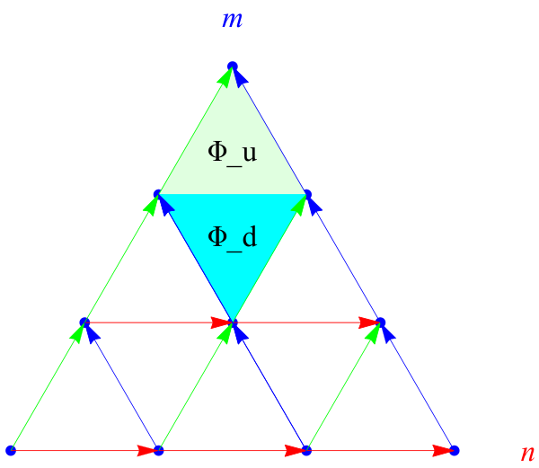
We illustrate the method for the Hofstadter models on the triangular lattice [13]. In a triangular lattice there is a freedom to tune the fluxes in the up and down triangles, . This freedom allows for making various plots of infinitely many different butterflies. We have chosen to consider the case where the vertical axis in Fig. 1 is the total flux and is fixed. We picked this particular value for because it gives the butterfly inversion symmetry. It lacks the reflection symmetry of the rectangular and hexagonal lattices.
The Diophantine equation can be read as an assignment of a gap index to a given Chern number. The resolution of the ambiguity for a gap index is obvious, since . The ambiguity problem for is now hidden in the fact that we do not know if a given , (rather than ) actually occurs. We know that occurs. This suggests the heuristics that small Chern numbers occur. This is equivalent to saying that Eq. (1.3) holds for and fails for . An argument in favor of this heuristics can be made if one thinks of the Chern number as edge modes [4]. Generically, one expects edge modes to gap out so that their number is small.
Asssuming this heuristics, the Diophantine equation can be written graphically as
| (1.5) |
which resolves the ambiguity for small Chern numbers . When the Chern number are the assignment from the left and right in Eq. (1.5) disagree reflecting the mod ambiguity.

Fig. 1, for the triangular lattice with , was plotted assuming the shifted window condition
| (1.6) |
The window appears to be free from major coloring errors. On the scale of few pixels, it becomes difficult to tell if the coloring is indeed right. The points were excluded because they lead to coloring errors illustrated in Fig. 3.
We have also numerically computing the Chern numbers, Eq. (C.3) for few pairs with small and found:
| (1.7) |
This shows that there are pairs for which the Chern numbers do not lie in any contiguous window.
There are topological obstructions to deformations Hofstadter models on the triangular lattice with to the square lattice: The two models are not adiabatically connected. This is true even if one restricts oneself to odd where all the gaps in the square model are open: The windows in Eq. (1.3) is incompatible with Eq. (1.6) and Eq. ( 1.7). Most have gaps that must close. For example, the fragmented window , results from a deformation of the contiguous window upon gap closure taking .
Conjecture 1.1
The mod ambiguity in the solution of Eq. (1.2) is, for generic Hofstadter models, a sign ambiguity: The Chern number is either the smallest positive or the smallest negative solution of the Diophantine equation. Equivalently: .
The conjecture is related to interesting separate problem namely, how to determine the sign of Chern numbers. Determining the sign of an integral is, of course, a much easier problem than evaluating it and can be estimated, with high probability using Monte-Carlo methods. In fact, for small gaps, the sign of the Chern number is likely to be the sign of the curvature at the gap edged. If the conjecture was true, it would allow for efficient algorithms for plotting high resolution Hofstadter butterflies when the resolution of the Mod ambiguity is not known.
In the appendixes we collect the tools we have used in the analysis.
Acknowledgment The research was supported by ISF. JA thanks Chris Marx, I. Dana, G. M. Graf and O. Zilberberg for useful discussions.
Appendix A Hofstadter models on triangular lattice
Define magnetic hopping on the triangular lattice,
| (A.1) |
See Fig. 4 for the meaning of , and the coordinates . The unitary accumulated by going (clockwise) around the up/down triangles are and around the unit cell :
A (tight-binding) Hofstadter model with isotropic hopping amplitudes is
| (A.2) |
A.1 : Inversion symmetry
Hofstadter models on the triangular lattice give the freedom to choose independently the fluxes in the up and down triangles. We have used this freedom to pick a model which is nice and symmetric.
The anti-unitary
acts on by
| (A.3) |
In a Hofstadter butterfly one looks at the spectrum as a function of the total flux . It follows that corresponds to a butterfly with inversion symmetry of the two axes of the diagram: , a symmetry evident in the Fig. 1.
A.2 Reduction to one dimension
The operators of Eq. (A.1) are independent of the coordinate . The symmetry allows reducing the problem from two dimensions, , to one dimension, . Let and act on the one dimensional lattice by
| (A.4) |
Take labeled by the conserved (quasi) momentum . One readily verifies that the action of on such functions takes the form
The Hofstadter Hamiltonian on has been reduced to a periodic family of Hamiltonians, labeled by , acting on :
| (A.5) |
A.3 Reduction to matrices
generates translations and since it commutes with itself it is translation invariant. is not. However, when , a rational root of unity, . is then periodic with period . This allows the reduction of the operator acting on to a matrix parametrized by two quasi-momenta .
A.4 Magnetic symmetry
The matrix is not a periodic function on the (magnetic) BZ. However, it is periodic up to a unitary transformation. In fact, there is a larger symmetry, known as “magnetic symmetry” [21].
The commutation of and , Eq. (A.9), imply
| (A.10) |
Since has a modular inverse which we denote by . Iterating Eq. (A.10) times give
| (A.11) |
It follows that the spectral properties are fully determined by a small square in the BZ, , whose size is .
A.5
The gauge transformation (diagonal unitary)
maps the building blocks
is manifestly periodic on . It follows that
| (A.12) |
is periodic on the BZ and
| (A.13) |
A.6 Discrete Fourier
and are discrete Fourier duals:
where the (discrete, not quite canonical) Fourier transform is the unitary matrix
Appendix B Chambers relation and band edges
An efficient computation of the spectrum of Hofstadter models can be made provided there is a-priori knowledge where in the BZ band edges occur. There is no known method to do that for general Hofstadter models, but Hofstadter models associated with tri-diagonal matrices are special. They admit Chambers relation [6, 12, 2] which facilitates this. Chambers formula says that characteristic polynomial takes the form
| (B.1) |
is a polynomial in of degree which is independent of . This says that for all and , band edges occur at the extremal points of
For the triangular lattice with different fluxes in the up/down triangles [2] determined :
B.1 Chambers formula
The characteristic polynomial of and coincide. Consider first its dependence. Since appears only in the two corners of the matrix, the dependence can be easily isolated by expanding in the first column (and then the first row). This gives Eq. (B.1) for with
| (B.2) |
The product with given in Eq.(A.13), can be evaluated explicitly
| (B.3) |
In the third line we used the fact that roots of unity sum to zero. In the last line we used the fact that come in conjugate pairs so their product is if is odd and if is even. Hence
The duality of and under Fourier, and the unitarity of Fourier, say that the same formula holds for . This gives for the triangular lattice [2]:
| (B.4) |
B.2 Band edges for
For the extremal points of Eq. (B.4) are determined by:
- 1.
odd: The maximum and minimum of
(B.5) The band edges occur at
(B.6) - 2.
even: The maximum and minimum of
(B.7) The band edges occur at
(B.8)
Appendix C Chern numbers
The adiabatic curvature of the n-th band is defined as [5]
| (C.1) |
The Chern number associated with the -th band is defined by [20]
| (C.2) |
The integration is over the (magnetic) Brillouin zone. It is known to be an integer [20]. Using the magnetic symmetry, Section (A.4), it can be written as [20]
| (C.3) |
by Stokes formula.
C.1 Chern numbers for gaps
The Chern number for the j-th gap is defined as the sum of Chern numbers of the bands below the gap:
| (C.4) |
The summand in Eq. (C.1) is anti-symmetric under . It follows that
| (C.5) |
In the Hofstadter model, Eq. (A.7), is a sum of six unitary operators and so . It follows that with the gap
The area of BZ is and hence
| (C.6) |
Appendix D Diophantine equation
The n-th band is associated with a projection . We shall supress to simplify the notation. is determined by the Hamiltonian and inherits its symmetries. In particular, is periodic, with period , up to the unitaries and as per Eqs. (A.11).
The Chern number of the n-th band is, by Eq. (C.3), times the holonoly in the phase of as one parallel transports the state around the square
A parallel transport that keeps the Berry’s phase, without accumulating a “dynamical phase” is given by the solution of the differential equation [15]
| (D.1) |
This evolution equation guarantees that stays in , i.e. all along the path: It satisfies the adiabatic theorem with no error.
Let be the solution of Eq. (D.1) along the open path . This defines a phase by
| (D.2) |
Similarly, let be the solution of Eq. (D.1) along the path . It defines a phase by
| (D.3) |
Now, we can get two different determinations of , one along the path and the other along the path . The discrepancy in the phases is the holonomy in phase associated with going around the square. This phase is precisely the value of the integral in Eq. (C.3), which we are after.
By the magnetic symmetry, Eqs. (A.11), parallel transport along the path assigns the phase
| (D.4) |
Similarly, parallel transport along the path assigns a different phase to the same state
| (D.5) |
Inserting Eq. (D.2) and Eq. (D.3) in Eq. (D.4) and Eq. (D.5) we find that the disagreement (holonomy) between these two assignments is
| (D.6) |
It follows from this and Eq. (C.3) that the Chern number of a single non degenerate band satisfies the Diophantine equation:
This completes the proof of the Diophantine equation.
References
- [1] Joseph E Avron, Daniel Osadchy, and Ruedi Seiler. A topological look at the quantum hall effect. Physics today, 56(8):38–42, 2003.
- [2] J Bellissard, C Kreft, and R Seiler. Analysis of the spectrum of a particle on a triangular lattice with two magnetic fluxes by algebraic and numerical methods. Journal of Physics A: Mathematical and General, 24(10):2329, 1991.
- [3] J Bellissard and B Simon. Cantor spectrum for the almost mathieu equation. Journal of Functional Analysis, 48(3):408 – 419, 1982.
- [4] B. Andrei Bernevig and Taylor L. Hughes. Topological Insulators and Topological Superconductors. Princeton University Press, 2013.
- [5] M.V. Berry. Quantal phase factors accompanying adiabatic changes. Proceedings of the Royal Society A, 392:45–57, 1984.
- [6] W. G. Chambers. Linear-network model for magnetic breakdown in two dimensions. Phys. Rev., 140:A135–A143, Oct 1965.
- [7] Man-Duen Choi, George A. Elliott, and Noriko Yui. Gauss polynomials and the rotation algebra. Inventiones Mathematicae, 99:225–246, 1990. 10.1007/BF01234419.
- [8] F. H. Claro and G. H. Wannier. Magnetic subband structure of electrons in hexagonal lattices. Phys. Rev. B, 19:6068–6074, Jun 1979.
- [9] I Dana, Y Avron, and J Zak. Quantised hall conductance in a perfect crystal. Journal of Physics C: Solid State Physics, 18(22):L679, 1985.
- [10] S. Friedland, J. W. Robbin, and J. H. Sylvester. On the crossing rule. Communications on Pure and Applied Mathematics, 37(1):19–37, 1984.
- [11] G.M. Graf, Private communication
- [12] J. H. Han, D. J. Thouless, H. Hiramoto, and M. Kohmoto. Critical and bicritical properties of harper’s equation with next-nearest-neighbor coupling. Phys. Rev. B, 50:11365–11380, Oct 1994.
- [13] Y. Hatsugai and M. Kohmoto. Energy spectrum and the quantum hall effect on the square lattice with next-nearest-neighbor hopping. Phys. Rev. B, 42:8282–8294, Nov 1990.
- [14] Yasuhiro Hatsugai, Takahiro Fukui, and Hideo Aoki. Topological analysis of the quantum hall effect in graphene: Dirac-fermi transition across van hove singularities and edge versus bulk quantum numbers. Phys. Rev. B, 74:205414, Nov 2006.
- [15] T. Kato. On the adiabatic theorem of quantum mechanics. J. Phys. Soc. Japan, 5:435–439, 1950.
- [16] Yaacov E. Kraus, Yoav Lahini, Zohar Ringel, Mor Verbin, and Oded Zilberberg. Topological states and adiabatic pumping in quasicrystals. Phys. Rev. Lett., 109:106402, Sep 2012.
- [17] K. A. Madsen, E. J. Bergholtz, and P. W. Brouwer. Topological equivalence of crystal and quasicrystal band structures. ArXiv e-prints, July 2013.
- [18] Pierre v Mouche. The coexistence problem for the discrete mathieu operator. Communications in mathematical physics, 122(1):23–33, 1989.
- [19] P Streda. Theory of quantised hall conductivity in two dimensions. Journal of Physics C: Solid State Physics, 15(22):L717, 1982.
- [20] D. J. Thouless, M. Kohmoto, M. P. Nightingale, and M. den Nijs. Quantized hall conductance in a two-dimensional periodic potential. Phys. Rev. Lett., 49:405–408, Aug 1982.
- [21] J. Zak. Magnetic Translation Group. Physical Review, 134:1602–1606, June 1964.