Compact Relaxations for MAP Inference in Pairwise MRFs with Piecewise Linear Priors
Abstract
Label assignment problems with large state spaces are important tasks especially in computer vision. Often the pairwise interaction (or smoothness prior) between labels assigned at adjacent nodes (or pixels) can be described as a function of the label difference. Exact inference in such labeling tasks is still difficult, and therefore approximate inference methods based on a linear programming (LP) relaxation are commonly used in practice. In this work we study how compact linear programs can be constructed for general piecwise linear smoothness priors. The number of unknowns is ) per pairwise clique in terms of the state space size and the number of linear segments . This compares to an size complexity of the standard LP relaxation if the piecewise linear structure is ignored. Our compact construction and the standard LP relaxation are equivalent and lead to the same (approximate) label assignment.
1 Introduction
Determining a maximum a-posteriori (MAP) solution in graphical models over discrete states, or equivalently finding a minimizer of a corresponding energy, is one of the fundamental tools in machine learning and computer vision. In this work we focus on problems with at most pairwise cliques (and associated pairwise potentials) in the graphical model. In the following we use the terms “pairwise potential” and “(smoothness) prior” synonymously. Since exact inference in graphical models (even with at most pairwise potentials) is generally not tractable, research has been focused on tractable and high-quality approximate inference algorithms, of which the linear programming (LP) relaxation for discrete inference tasks (e.g. [4, 22, 21, 20]) has received much attention. In some cases the LP relaxation solves the inference problem exactly [10, 13, 18], i.e. the relaxation is tight for certain problem classes. Due to the specific structure of the resulting linear program generic methods to solve linear programs are inefficient and therefore many specialized algorithms to find a minimizer have been proposed in the literature. Since the primal linear program for MAP estimation in pairwise problems has a quadratic number of unknowns in terms of the state space size (per edge in the underlying graph), the dual program with only a linear number of unknowns (but with a quadratic number of e.g. constraints) is more appealing. Belief propagation inspired message passing methods optimize this dual program in a block-coordinate schedule [14, 12, 6, 8]. As block-coordinate methods applied on a non-smooth and not strictly concave problem these approaches iteratively increase the dual objective but are not guaranteed to find a global maximizer of the (concave dual) problem. This is well known in the literature, and we validate this occasional “early stopping” behavior in the experimental section. Supergradient methods with an appropriate stepsize rule are guaranteed to converge to a maximizer, but have a slow convergence rate (where is the iteration count). To our knowledge all variations of faster proximal methods explicitly or implicitly maintain primal unknowns, and are therefore prohibitively expensive (in terms of memory requirements) for large state spaces. Variable smoothing methods for non-smooth problems (e.g. [1]) have an convergence rate and require only unknowns if applied on the dual problem, but in practice show slow convergence in our experience (as verified in our experimental section).
A natural question is whether the size of the primal program can be reduced if the pairwise potentials are not arbitrary but have some useful “structure.” For particular pairwise potentials such as the -norm of label differences [11, 2] or truncated priors [26] the answer is affirmative. We generalize these particular results to pairwise potentials that are piecewise linear in terms of the label difference. In many computer vision related inference problems the state space is a set of numeric values and the employed smoothness prior is naturally based on label value differences. Some of the potentials addressed in our work are illustrated in Fig. 1. We show that for such pairwise potentials (but with arbitrary unary ones) we can reformulate the primal linear programs in order to reduce the number of primal variables from to , where is the number of linear pieces defining the pairwise potential. The number of dual unknowns (or primal constraints, respectively) increases to , meaning an overall problem size. Specifically, we consider pairwise potentials that can be written as pointwise minimum of convex ones. Since our construction is a reformulation, there is a correspondence between minimizers of the original LP and the ones from our reduced program. Thus, our construction does not weaken the LP relaxation for inference.
This manuscript is organized as follows: after introducing relevant notations and briefly reviewing approximate MAP inference in Section 2, we state our main result in Section 3. The corresponding proof is constructive and the two main ingredients are presented in Sections 4 (convex pairwise priors) and 5 (pointwise minimum of pairwise potentials), respectively. Since the underlying techniques are useful in their own right, we provide the material in separate (and relatively self-contained) sections. In Section 6 we discuss extensions of the proposed reformulations to enable more isotropic behavior of solutions, which can be relevant in image processing applications. In Section 7 we experimentally verify that message passing methods can stop early, and we demonstrate our approach in an image denoising experiment.
2 Background
In this section we introduce some notation used throughout the manuscript, and further provide a short review on approximate inference for labeling problems.
2.1 Notations
The domain of the considered label assignment task is a graph with node set and edge set . In computer vision and image processing applications the node set is typically a regular pixel grid and is induced by a e.g. 4-connected or 8-connected neighborhood structure. We will write and as shorthand notations for and , respectively. Our convention is that , denote nodes from and , indicate states (or labels). We will also use the sets for the successor of and for the ancestor nodes of .
The -dimensional (unit or probability) simplex is defined as . Elements can be seen as discrete probability densities, and we denote the corresponding cumulative distribution function with . We extend to indices with for and for . If is integral (e.g. for some , and 0 otherwise), then can also be interpreted as superlevel function with . The main purpose of introducing is to have a shorthand notation for , which will occur frequently in this manuscript.
We use the notations and to write a constraint as an extended valued function, i.e. is 0 iff and otherwise. For a convex function we denote its convex conjugate by and the l.s.c. extension of its perspective as , which can be defined via the biconjugate:
| (1) |
Throughout the manuscript we assume that the recession function of is (i.e. ). This can be achieved by adding redundant bounds constraints to , since all unknowns in our convex problems are usually restricted to . In section 5 we will make use of the following fact (see e.g. [27]):
Lemma 1.
Let be a family of convex functions, then
| (2) |
2.2 Approximate Inference
For a given graph and label (state) space the task of inference in a label assignment problem is to determine a minimizer of
| (3) |
where (a mapping from nodes to states), and and are the unary and pairwise potentials, respectively. The local nature of the modeled interactions means that the above label assignment problem is an instance of a Markov Random Field (MRF). Note that with respect to inference (i.e. finding a MAP solution) conditional random fields (CRFs) are completely equivalent to MRFs, and our use of the term “MRF” includes both CRFs and “proper” MRFs. In this work we focus on problems with at most pairwise interactions between labels. In general such labeling problems are difficult to solve exactly due to the NP-hardness of many instances. A tractable approximation to is obtained by “lifting” the problem to a higher dimensional setting: for each node and each edge vectors and are introduced, which denote “soft one-hot” encodings of the labels assigned to a node (or to an edge, respectively) (see e.g. [22, 21, 20]). As result one obtains the following linear programming relaxation enabling tractable approximate inference:
| (4) | ||||
| subject to | ||||
The first set of constraints are usually called marginalization constraints. These constraints ensure that the labels assigned to edges are consistent with the ones assigned at nodes. implies the normalization constraint .
In many computer vision problems (e.g image denoising, optical flow) the pairwise terms often do not depend on the actual labels and but only on their difference (i.e. the “height” of jumps between labels). In this case the pairwise potentials can be written as , or even as in the case of symmetric ones.
The number of unknowns in Eq. 4 is in which can make inference with many labels costly. For certain pairwise potentials the number of unknowns can be reduced to , e.g. potentials (, [11, 2]), and truncated potentials (, e.g. [26]). In this work we show that the number of primal unknowns can be reduced from to for piecewise linear potentials consisting of segments.
3 The Main Result
In this section we state our main result, which generically shows that piecewise linear pairwise potentials allow for a compact reformulation of (Eq. 4). In this section we only sketch the proof, since it is based on more general constructions described in detail in Sections 4 and 5.
Theorem 1.
Let be a pairwise potential, that is a piecewise linear function with respect to consisting of segments, having breakpoints only at integral values of . Then there exists a reformulation of Eq.4 that requires primal unknowns and linear constraints per edge in the graph.
Proof.
(Sketch:) In the following we consider a particular edge and drop the subscript . Under the above assumptions on can be written as
| (5) |
i.e. as minimum of linear functions with bounded (and convex) domains (see Fig. 2). Using the results derived in Section 4, potentials of the form
| (6) |
allow for a compact reformulation of Eq. 4 using only primal unknowns and at most constraints (see Eq. 17). In Section 5 it is shown that the minimum of such potentials (represented by their compact reformulations) leads to a combined reformulation with unknowns and constraints (see Eq. 28). ∎
Remark 1.
Our way of counting constraints corresponds to the number of dual variables one needs to introduce in order to obtain a convenient saddle-point formulation suitable for straightforward optimization e.g. via the (preconditioned) primal-dual method [17]. Therefore we do not need to introduce dual variables whenever closed-form proximal steps are available. In particular, we do not include simple bounds constraints (such as non-negativity constraints) in our counting of constraints, but we always introduce enough dual variables to avoid non-trivial proximal steps.
Remark 2.
We want to emphasis that rewriting piecewise linear potentials as minimum of bounded linear functions (as in Eq. 5) also allows for efficient updates in message passing algorithms (such as belief propagation and its variants with guaranteed convergence). Efficient methods addressing (optionally truncated) and quadratic regularization are already presented in [5], and we can easily generalize their result: assume the pairwise potentials can be written as minimum of simple convex potentials as in Eq. 5, then the lower envelope computation
| (7) |
can be done in time. This can be seen as follows: we rewrite the minimum envelope as
hence the minimum envelope can be computed in time if the inner envelope can be done in time. Observe that the lower envelope
is an instance of the min-filter problem, which can be solved in time (e.g. [23]). Interestingly, the very easily implementable online algorithm for min-filtering proposed in [15] clearly resembles the lower envelope algorithm for quadratic costs in [5].
4 Piecewise Linear and Convex Pairwise Potentials
In this section we consider pairwise potentials, that can be written as pointwise maximum of affine functions in terms of the label difference , i.e.
| (8) |
for parameters , . We assume that the breakpoints of as a function of are located on integral arguments . Since pairwise potentials are only specified for integral label values, this can be always achieved (at the expense of at most doubling the number of affine functions).
In order to simplify the notation we assume w.l.o.g. edge-independent values and (and therefore drop the subscript ), but all results below hold for edge-specific coefficients and as well. By definition is a convex and piecewise linear function with respect to , see also Fig. 1(a).
4.1 Minimum Cut Graph Construction
Our construction below is different to Ishikawa’s graph cut approach solving MRFs with convex and symmetric priors [10], but can be seen as generalization of his earlier construction in [11]. The main benefits of our proposed construction can be summarized as follows: first, it is very intuitive to understand; second, it naturally allows asymmetric convex potentials; and finally, it immediately enables extensions to more isotropic regularizers that can be relevant in image processing applications.
The labeling problem with convex pairwise priors is solved by computing the minimum-cut in a weighted graph. The node set of the graph is , where and are the source and sink, respectively. The edge set contains infinity links and for all . Node is connected to node with a directed edge . A label is assigned to if the minimal cut goes through edge . In order to ensure that only one label is assigned at a node , there are directed edges with infinite weight from nodes to . Finally, a subset of directed pairwise edges connecting with (and vice versa) will be included into the graph as described in the following.
The convex potential in Eq. 8 can be equivalently written as (with )
| (9) |
It will be convenient later to explicitly include the affine term, . Note that only affects the objective of the minimizer, not the minimizer itself, and hence can be ignored in the graph construction. The term does not depend jointly on and , and consequently can be (temporarily) absorbed into the unary potentials for the graph construction (e.g. and are augmented with and , respectively). Thus, we focus on the first expression in Eq. 9 below.
With our above assumption of integral breakpoints we have without loss of generality. In the following we focus on a single summand, . If , the term corresponds to a “one-sided” (or total variation) regularizer and can be solved by adding lateral directed edges into the graph (see Fig. 3(a)). If , one can temporarily reinterpret label value as and again obtain an asymmetric -type smoothness prior but between label and a “shifted” label . Consequently, for each term with directed diagonal edges are inserted into the graph (see Fig. 3(b)).
4.2 The Equivalent Linear Program
The resulting graph can be immediately written as linear program11 1 The expressions appearing in the objective can be removed leading to a proper LP after introducing a non-negative with . ,
| (10) | ||||
| s. t. |
where encodes whether node belongs to the source () or to the sink (). Note that we explicitly state the contribution of the linear part, in Eq. 9, to the unaries. In order to keep the equations simple, we introduce the convention that “out-of-bounds” values yield 0 if and 1 if for all .
Observe that as function of is a superlevel representation and can therefore be written as for some . Thus, we can rewrite as
| (11) | ||||
| s.t. |
In order to use this result as a building block for the construction in the following Section 5, we introduce for the pairwise terms
| (12) | ||||
We explicitly added the (redundant) simplex constraints on and in order to obtain a trivial recession function for , which will be important in Section 5. Now, can be rewritten as
| (13) |
subject to . Observe that introduces unknowns, and , per edge , and enforces constraints (where we identify with one inequality constraint). Of course, the extra unknowns, and , and of the constraints can be discarded immediately by applying e.g. the constraint , but as stated in Eq. 12 will be important in Section 5.
Overall, depending on the values of and optimization of potentially requires far less memory than optimizing the generic LP relaxation (Eq. 4). A particular and important instance of convex potentials are -type ones, . For completeness we state one respective specialization of to :
| (14) |
4.3 Linear Priors with Bounded Domains
In this section we discuss the particular prior relevant for the main result in Section 3, where specific convex potentials of the shape
| (15) |
(with being a sufficiently large constant) are considered. In this particular setting (Eq. 12) reads as
| (16) | ||||
subject to . With the penalizer terms transform into constraints and (which correspond to infinity links in the respective minimum-cut graph), and therefore equivalently reads as
| (17) | ||||
and by plugging as into Eq. 13 we obtain a program with unknowns per edge and at most constraints (or dual variables) as claimed in the proof of Theorem 1.
5 Minimum of Pairwise Potentials
In this section we show that the (pointwise) minimum of compactly representable pairwise potentials leads again to a compact representation of the corresponding linear program. This applies e.g. to pairwise potentials that are the minimum of (not necessarily symmetric) -type pairwise priors (see Fig. 1(b)). It is well-known that -type priors lead to linear programs with unknowns per edge (e.g. [11], or apply the result from the previous section). A corollary from the construction presented in the following is, that the minimum of -type priors only requires primal unknowns without loosening the convex relaxation, compared to . We will call the pointwise minimum of pairwise “elementary” potentials a “min-potential” in the following.
In order to show the equivalence of a compact linear program for min-potentials with the standard relaxation (Eq. 4) we proceed in two steps:
- •
- •
If the elementary potentials are chosen such that they have a compact reformulation (as the ones discussed in Section 4), one can substitute the elementary potentials by their corresponding compact reformulation. In Section 5.2 the equivalence of the resulting reformulation is shown, and some relevant examples are provided.
Overall, the equivalence of (Eq. 4) with compact reformulations is thus established.
The following derivations make repeated use of Lemma 1, which allows us to rewrite a minimum of convex functions as convex minimization problem in general. Application of Lemma 1 on the terms representing elementary potentials in order to obtain min-potentials leads to non-convex bilinear constraints as shown below. The following lemma states in a general setting, that these bilinear constraints induced by application of Lemma 1 can be “linearized” without affecting the minimum.
Lemma 2.
Let be a family of convex l.s.c. functions (with trivial recession function). Further define the following minimization problems,
We have that
| (18) |
Proof.
The equivalence of and follows immediately from Lemma 1. The equality is shown as follows: observe that , since any feasible for is also feasible for (summing all constraints over and using implies ).
To prove we consider the Lagrangian duals of the two convex programs. We have (also applying Lemma 1)
Analogously we obtain
Both dual programs have essentially the same objective , but enforces additional constraints on its argument ( for some ), from which the already known fact follows. But any maximizer of can be converted to a feasible solution of with the same objective by setting , where
Therefore both the dual programs have the same optimal value, and follows from strong duality. ∎
In the following we repeatedly apply Lemma 2 to obtain compact and convex reformulations for min-potentials. The node variables and involved in the pairwise potentials via the marginalization constraints (or a respective variant) will attain the role of in the lemma. Since these node variables are subject to optimization as well (on the outer scope), Lemma 2 is important to replace occuring bilinear constraints by linear ones.
5.1 Term-Wise Minimum of Potentials
Let the pairwise potentials be written as pointwise minimum of elementary potentials , i.e.
In this section we show the equivalence of
| (19) | ||||
| s. t. | ||||
and
| (20) | ||||
| s. t. | ||||
Note that the difference between the two programs is the position of . In a new pairwise potential is formed as the point-wise minimum of given ones,
| (21) |
whereas in a particular active potential is selected per edge (see also Fig. 4). The equivalence of the two energies is an immediate consequence of the following fact:
Lemma 3.
For given and let denote the (local) marginalization constraints
The following two pairwise costs
and
are equivalent, i.e.
| (22) |
Proof.
First we remark that obviously , since a sum of pointwise minima is never larger than the minimum of sums (over the same terms). In order to show we rewrite
with
Observe that the recession function of is trivial due to the simplex constraint . Thus, we can apply Lemma 2 on to obtain an equivalent convex program,
We substitute in (leading to the constraint , or combined with , to ),
Let be a minimizer of , and let . We set iff and 0 otherwise. Then is feasible for and has the same objective value as . Consequently, , and since and are equivalent. Overall, we have as claimed. ∎
The equivalence of and means that given pairwise potentials than can be written as pointwise minimum of some “convenient” elementary potentials, we can focus our attention on compact representations of these elementary potentials.
5.2 Term-Wise Minimum of Compact Potentials
In this section we assume that elementary pairwise potentials have a more compact equivalent, e.g.
for some convex function (having a trivial recession function). The respective non-convex labeling energy reads as
| (23) | ||||
and we use Lemma 2 below to obtain an equivalent convex program. For concreteness, and due to the important of piecewise convex pairwise potentials, we instantiate with (recall Eq. 12) in our derivation,
| (24) | ||||
In order to apply Lemma 2 we need the perspective of , which can be immediately stated as
| (25) |
Application of Lemma 2 (with the constraints and taking the role of the constraint “”) establishes the equivalence of
and
| (26) |
subject to
The occuring variables have intuitive meanings: is a (soft) one-hot encoding of which branch is active in , i.e. represents the set . It is easy to see that for all values of and a minimizer will attain only binary values (it can also be fractional if contains more than one element). and represent and , respectively (as “local copies”), in the -th branch.
If the above expressions are plugged into Eq. 23, and the edge-specific unknowns etc. are augmented with the respective edge subscript , one obtains the energy given in Eq. 27. If we specialize to be the linear but bounded potentials (Eq. 16) and express in terms of (e.g. ), we arrive at the convex program given in Eq. 28 relevant for the main result in Theorem 1. One can directly read off the number of unknowns per edge (which is ) and constraints (dual variables, at most ) from the resulting program.
For practical implementations it can be beneficial to implement specializations of rather than . For instance, if the smoothness prior is the minimum of -type potentials, a generic implementation based on (which models the potential via linear segments) requires about twice the number of unknowns and constraints than a specific formulation (depicted in Eq. 29) derived from and (Eq. 14).22 2 If we assume the solver can directly cope with , which is the case e.g. for proximal methods-based implementations.
| (27) |
| s.t. | |||||||
| (28) |
| s.t. | |||||||||
| (29) |
| s.t. | |||||||
6 Reducing the Grid Bias
Until now we restricted the exposition to labeling tasks with underlying discrete (i.e. graph structured) domains. In some cases continuously inspired label assignment formulations (e.g. [3]) are preferable in image processing and computer vision problems due to the reduced metrication artifacts. As pointed out in [25, 26] the finite difference discretization of continuous formulations is closely related to standard LP relaxations for inference such as (Eq. 4). In a nutshell, continuously inspired labeling formulation replace linear smoothness terms (i.e. in ) with nonlinear, Euclidean-norm based terms in order to achieve better counting of non grid-aligned discontinuities.
We follow existing literature and use a forward difference stencil in the following. We expect slightly improved visual results if the discretization of the image plane is based on e.g. a staggered grid or uses a discrete calculus formulation [7]. In our finite difference setting the image domain is represented by a regular grid with horizontal and vertical edges between pixels. We index horizontal edges with subscripts (where is the left grid point of the edge) and vertical ones with (see also Fig. 8). Thus, e.g. variables and represent depending whether is a horizontal or vertical edge. For notational simplicity we assume homogeneous and symmetric pairwise potentials in the following (i.e. we drop edge subscripts in the coefficients, and assume ). The simplest isotropic extension shown in Eq. 30 replaces the separate, -type counting of horizontal and vertical discontinuities in Eq. 27, e.g. terms such as
with a joint Euclidean-norm penalizer,
Consequently, edges cut jointly in horizontal and vertical direction imply a increase in the smoothness term, which corresponds to the standard -length penalization of diagonal discontinuities.
Similar reasoning holds for the constant cost in (Eq. 24, which translates to the term in Eq. 27). We also replace the -type contribution
(since ) with an Euclidean cost,
and the complete objective is given in (Eq. 30). In Eq. 31 we further depict the convex program in analogy to the anisotropic energy (Eq. 29).
Our choice for the isotropic extension reduces to approaches presented in the literature such as isotropic potentials [16], Potts smoothness prior [24], and truncated priors [26]. The construction is described for 2D image domains but can obviously be extended to higher dimensional image domains.
| (30) |
| s.t. | |||||||||||
| (31) |
subject to the same constraints as in Eq. 30.
Remark 3.
In order to reduce the metrication artifacts for min-potentials one has two options: the first option is to convert an anisotropic formulation, e.g. Eq. 27, to behave “less anisotropic.” This is the approach as presented above. The other option is to use isotropic formulations as elementary potentials and subsequently apply the construction described in Section 5 to obtain the minimum potential. If we focus on the minimum of -type (total variation) potentials, and if we employ the standard forward-difference discretization, the underlying elementary potential is given by
| (32) |
where nodes , , and form a neighborhood as shown in Fig. 8. Application of Lemma 2 to rewrite terms
| (33) |
leads to the convex program Eq. 34. It can be observed from the resulting constraints, that in this formulation e.g. the same elementary potential needs to be selected in horizontal and vertical direction. Further, the “constants” are counted differently in and . We currently prefer , since it reduces to the Potts and truncated models presented in the literature, but a deeper analysis is subject of future research.
| (34) |
| s.t. | |||||||||
7 Numerical Results
Unless otherwise noted we use a straightforward OpenMP-parallelized C++ implementation of the first order primal-dual method described in [17] to find minimizers of the respective convex program. As with other proximal methods the algorithm leaves freedom of how the convex problem is splitted (i.e. which dual unknowns are introduced, and the choice of proximal steps utilized). The employed splitting often has a significant impact on convergence behavior. In general, we eliminate from the objective and introduce Lagrange multipliers for each of the remaining constraints. We also introduce bounds-constrained dual variables for terms as
A naive implementation of the respective primal-dual update steps has a time complexity (per edge in the graph), and we use appropriate running sums to preserve the complexity.
7.1 Early Stopping of Message Passing Methods
As first experiment we verify the claim that early stopping can occur frequently in dual block coordinate methods for MAP inference such as MPLP [6]. We follow the setup of a similar experiment described in [19], but replace the 3-label spin glass model considered there by problem instances with many labels and piecewise linear smoothness priors. Our setup is as follows: the domain is a regular grid with the standard 4-connected neighborhood stucture, and the state space contains 20 labels. The unary potentials are sampled randomly from a uniform distribution , and the pairwise potentials are truncated linear ones with
| (35) |
and are used. We solve 300 random instances using MPLP and compare the energy to the globally optimal one obtained by minimizing using the primal-dual algorithm. In about of the problem instances MPLP stops early with an energy difference of more than 0.001 and in about with more than 0.01 (see also Fig. 12).
7.2 Variable Smoothing
Recent developments in accelerated gradient methods (e.g. [1]) appear to be very appealing in order to optimize the non-smooth dual program of e.g. (Eq. 4). The method proposed in [1] guarantees an convergence rate, where is the iteration count, but requires to set a tuning parameter. In Fig. 13 it is illustrated that this parameter has to be chosen carefully to achieve competitive performance. Our conclusion is that such variable smoothing methods cannot (yet) replace compact reformulations as proposed in the previous sections.
7.3 Convergence Speed and Memory Consumption
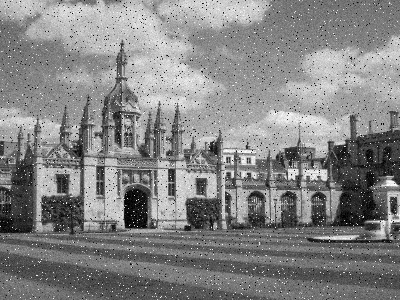
We use a more realistic application to compare memory requirements and the evolution of energies. While a compact reformulation such as has a smaller problem size than , it is not clear whether the more complicated problem structure may lead to slower convergence. We chose a simple image denoising application for this demonstration. We use a piecewise linear approximation depicted in Fig. 14(b) of the gradient statistic of natural images [9]. The unary potential (shown in Fig. 14(a)) is induced directly by our image corruption procedure, which is as follows: a random set containing five percent of the pixels are considered as outliers and their clean intensity values are replaced by a uniform random value from . For the remaining inlier pixels we add Gaussian noise drawn from to their respective clean intensities. Thus, the data fidelity term is given by
where is the density function of the Normal distribution. We set , and the utilized regularizer (Fig. 14(b)) is
with , , and . The observed noisy image is illustrated in Fig. 14(c), and the recovered image can be seen in Fig. 14(d). The solution image is determined by extracting the 1/2-isolevel of the superlevel function .
We discretize the continuous state space into 64 labels. The memory used to minimize for this problem is almost 8GB, and optimizing (, respectively) requires about 1.1GB memory. Hence, the latter formulations will fit in graphics memory and can therefore leverage GPUs for acceleration. The evolution of the objective is displayed in Fig. 15. All primal and dual unknowns are initialized with 0, which may explain the initial increase in the objective value. The compact reformulations / have a clear advantage over the exhaustive model .

7.4 Comparison with A Continuously-inspired Formulation
In [16] a continuous approach is described that addresses labeling problems with convex smoothness priors (in terms of the spatial gradient of the assigned label function) but arbitrary data fidelity term. It is further shown that in the continuum a global solution can be obtained by thresholding a minimizer of an underlying convex relaxation. This result does in general not hold after discretizing the continuous functional. An interesting example of a convex smoothness prior that is considered in [16] is the Lipschitz prior, for some . This regularizer enforces bounded label differences for adjacent nodes (pixels) and is very compact to represent in the framework of Section 4,
together with and . will be 32 in the following. Note that the energy formulation in [16] also requires only variables and constraints per edge in the grid. In order to have a ground truth result available for better comparison, we use a (convex) quadratic data term, , which implies that an optimal labeling can be easily obtained (see Figs. 16(a,d), we choose ). Figs. 16(b,e) depict the result of the discretized model [16] with the label space discretized into states, and Figs. 16(c,f) display the result of Eq. 30 specialized to . In terms of the PSNR our result is much closer to the true minimizer, and further preserves more image details. This small experiment indicates that often care is required when working with discretized problems of continuous labeling functionals.


8 Conclusion
We show that pairwise potentials, that can be written as piecewise linear functions in terms of the respective label difference, allow compact reformulations of the LP relaxation for MAP inference. These reformulations do not weaken the relaxation or modify the returned minimizer. The resulting savings in memory consumption can be very significant (e.g. one order of magnitude) for many-label problems. The construction also extends to formulations aiming to reduce the grid bias often used in image processing.
Future work will address the applicability of the underlying techniques developed in this manuscript to general piecewise linear potentials (not only those that can be written as ), and to higher order potentials beyond pairwise ones.
References
- [1] Radu Ioan Bot and Christopher Hendrich. A variable smoothing algorithm for solving convex optimization problems. arXiv preprint arXiv:1207.3254, 2012.
- [2] Y. Boykov, O. Veksler, and R. Zabih. Markov random fields with efficient approximations. In IEEE Conference on Computer Vision and Pattern Recognition (CVPR), pages 648–655, 1998.
- [3] Antonin Chambolle, Daniel Cremers, and Thomas Pock. A convex approach to minimal partitions. SIAM Journal on Imaging Sciences, 5(4):1113–1158, 2012.
- [4] Chandra Chekuri, Sanjeev Khanna, Joseph Naor, and Leonid Zosin. A linear programming formulation and approximation algorithms for the metric labeling problem. SIAM Journal on Discrete Mathematics, 18(3):608–625, 2004.
- [5] Pedro F Felzenszwalb and Daniel P Huttenlocher. Efficient belief propagation for early vision. Int. Journal of Computer Vision, 70(1):41–54, 2006.
- [6] Amir Globerson and Tommi Jaakkola. Fixing max-product: Convergent message passing algorithms for map lp-relaxations. Advances in neural information processing systems (NIPS), 21(1.6), 2007.
- [7] Leo John Grady and Jonathan R Polimeni. Discrete calculus: Applied analysis on graphs for computational science. Springer, 2010.
- [8] T. Hazan and A. Shashua. Norm-prodcut belief propagtion: Primal-dual message-passing for lp-relaxation and approximate-inference. IEEE Trans. on Information Theory, 56(12):6294–6316, 2010.
- [9] Jinggang Huang and David Mumford. Statistics of natural images and models. In IEEE Computer Society Conference on Computer Vision and Pattern Recognition (CVPR), volume 1. IEEE, 1999.
- [10] Hiroshi Ishikawa. Exact optimization for markov random fields with convex priors. IEEE Transactions on Pattern Analysis and Machine Intelligence (TPAMI), 25(10):1333–1336, 2003.
- [11] Hiroshi Ishikawa and Davi Geiger. Segmentation by grouping junctions. In IEEE Conference on Computer Vision and Pattern Recognition, pages 125–131. IEEE, 1998.
- [12] V. Kolmogorov. Convergent tree-reweighted message passing for energy minimization. IEEE Transactions on Pattern Analysis and Machine Intelligence (PAMI), 28(10):1568––1583, 2006.
- [13] V. Kolmogorov and M. Wainwright. On the optimality of tree-reweighted max-product message-passing. In Proc. Uncertainty in Artificial Intelligence (UAI), 2005.
- [14] V.A. Kovalevsky and V.K. Koval. A diffusion algorithm for decreasing energy of max-sum labeling problem. Glushkov Inst. of Cybernetics, Kiev, USSR, 1975.
- [15] Daniel Lemire. Streaming maximum-minimum filter using no more than three comparisons per element. Nordic J. Computing, 13(4):328–339, 2006.
- [16] T. Pock, D. Cremers, H. Bischof, and A. Chambolle. Global solutions of variational models with convex regularization. SIAM Journal on Imaging Sciences, 3(4):1122–1145, 2010.
- [17] Thomas Pock and Antonin Chambolle. Diagonal preconditioning for first order primal-dual algorithms in convex optimization. In IEEE International Conference on Computer Vision (ICCV), pages 1762–1769. IEEE, 2011.
- [18] D. Schlesinger. Exact solution of permuted submodular MinSum problems. In Proc. Energy Minimization Methods in Computer Vision and Pattern Recognition (EMMCVPR), pages 28–38, 2007.
- [19] Alex Schwing, Tamir Hazan, Marc Pollefeys, and Raquel Urtasun. Globally convergent dual map lp relaxation solvers using fenchel-young margins. In Advances in Neural Information Processing Systems (NIPS), pages 2393–2401, 2012.
- [20] D. Sontag, A. Globerson, and T. Jaakkola. Optimization for Machine Learning, chapter Introduction to Dual Decomposition for Inference. MIT Press, 2011.
- [21] M. J. Wainwright and M. I. Jordan. Graphical models, exponential families, and variational inference. Found. Trends Mach. Learn., 1:1–305, 2008.
- [22] T. Werner. A linear programming approach to max-sum problem: A review. IEEE Transactions on Pattern Analysis and Machine Intelligence (PAMI), 29(7), 2007.
- [23] Hao Yuan and Mikhail J Atallah. Running max/min filters using comparisons per sample. Pattern Analysis and Machine Intelligence, IEEE Transactions on, 33(12):2544–2548, 2011.
- [24] C. Zach, D. Gallup, J.-M. Frahm, and M. Niethammer. Fast global labeling for real-time stereo using multiple plane sweeps. In Proc. VMV, 2008.
- [25] C. Zach, C. Häne, and M. Pollefeys. What is optimized in tight convex relaxations for multi-label problems? In IEEE Conference on Computer Vision and Pattern Recognition (CVPR), 2012.
- [26] C. Zach, C. Häne, and M. Pollefeys. What is optimized in convex relaxations for multi-label problems: Connecting discrete and continuously-inspired MAP inference. IEEE Transactions on Pattern Analysis and Machine Intelligence (PAMI), 2013. accepted for publication.
- [27] Christopher Zach and Pushmeet Kohli. A convex discrete-continuous approach for markov random fields. In European Conference on Computer Vision (ECCV), pages 386–399. Springer Berlin Heidelberg, 2012.