Trace Complexity of Network Inference
Abstract
The network inference problem consists of reconstructing the edge set of a network given traces representing the chronology of infection times as epidemics spread through the network. This problem is a paradigmatic representative of prediction tasks in machine learning that require deducing a latent structure from observed patterns of activity in a network, which often require an unrealistically large number of resources (e.g., amount of available data, or computational time). A fundamental question is to understand which properties we can predict with a reasonable degree of accuracy with the available resources, and which we cannot. We define the trace complexity as the number of distinct traces required to achieve high fidelity in reconstructing the topology of the unobserved network or, more generally, some of its properties. We give algorithms that are competitive with, while being simpler and more efficient than, existing network inference approaches. Moreover, we prove that our algorithms are nearly optimal, by proving an information-theoretic lower bound on the number of traces that an optimal inference algorithm requires for performing this task in the general case. Given these strong lower bounds, we turn our attention to special cases, such as trees and bounded-degree graphs, and to property recovery tasks, such as reconstructing the degree distribution without inferring the network. We show that these problems require a much smaller (and more realistic) number of traces, making them potentially solvable in practice.
1 Introduction
Many technological, social, and biological phenomena are naturally modeled as the propagation of a contagion through a network. For instance, in the blogosphere, “memes” spread through an underlying social network of bloggers [2], and, in biology, a virus spreads over a population through a network of contacts [3]. In many such cases, an observer may not directly probe the underlying network structure, but may have access to the sequence of times at which the nodes are infected. Given one or more such records, or traces, and a probabilistic model of the epidemic process, we can hope to deduce the underlying graph structure or at least estimate some of its properties. This is the network inference problem, which researchers have studied extensively in recent years [2, 15, 14, 8, 23].
In this paper we focus on the number of traces that network inference tasks require, which we define as the trace complexity of the problem. Our work provides inference algorithms with rigorous upper bounds on their trace complexity, along with information-theoretic lower bounds. We consider network inference tasks under a diffusion model presented in [15], whose suitability for representing real-world cascading phenomena in networks is supported by empirical evidence. In short, the model consists of a random cascade process that starts at a single node of a network, and each edge independently propagates the epidemic, once is infected, with probability after a random incubation time.
Overview of results. In the first part of this paper, we focus on determining the number of traces that are necessary and/or sufficient to perfectly recover the edge set of the whole graph with high probability. We present algorithms and (almost) matching lower bounds for exact inference by showing that in the worst case, traces are necessary and traces are sufficient, where is the number of nodes in the network and is its maximum degree. In the second part, we consider a natural line of investigation, given the preceding strong lower bounds, where we ask whether exact inference is possible using a smaller number of traces for special classes of networks that frequently arise in the analysis of social and information networks. Accordingly, we present improved algorithms and trace complexity bounds for two such cases. We give a very simple and natural algorithm for exact inferences of trees that uses only traces.11 1 All inference results in this paper hold with high probability. To further pursue this point, we give an algorithm that exactly reconstructs graphs of degree bounded by using only traces, under the assumption that epidemics always spread throughout the whole graph. Finally, given that recovering the topology of a hidden network in the worst case requires an impractical number of traces, a natural question is whether some non-trivial property of the network can be accurately determined using a moderate number of traces. Accordingly, we present a highly efficient algorithm that, using vastly fewer traces than are necessary for reconstructing the entire edge set, reconstructs the degree distribution of the network with high fidelity by using traces.
The information contained in a trace. Our asymptotic results also provide some insight into the usefulness of information contained in a trace. Notice that the first two nodes of a trace unambiguously reveal one edge — the one that connects them. As we keep scanning a trace the signal becomes more and more blurred: the third node could be a neighbor of the first or of the second node, or both. The fourth node could be the neighbor of any nonempty subset of the first three nodes, and so on. The main technical challenge in our context is whether we can extract any useful information from the tail of a trace, i.e., the suffix consisting of all nodes from the second to the last. As it turns out, our lower bounds show that, for perfect inference on general connected graphs, the answer is “no”: we show that the First-Edge algorithm, which just returns the edges corresponding to the first two nodes in each trace and ignores the rest, is essentially optimal. This limitation precludes optimal algorithms with practical trace complexity22 2 On the other hand, the use of short traces may not be only a theoretical limitation, given the real world traces that we observe in modern social networks. For example, Bakshy et al. [4] report that most cascades in Twitter (twitter.com) are short, involving one or two hops.. This result motivates further exploration of trace complexity for special-case graphs. Accordingly, for trees and bounded degree graphs, we illustrate how the tail of traces can be extremely useful for network inference tasks.
Our aforementioned algorithms for special-case graphs make use of maximum likelihood estimation (MLE) but in different ways. Previous approaches, with which we compare our results, have also employed MLE for network inference. For instance, NetInf [15] is an algorithm that attempts to reconstruct the network from a set of independent traces by exploring a submodular property of its MLE formulation. Another example, and closest to ours, is the work by Netrapalli and Sangahvi [23], whose results include qualitatively similar bounds on trace complexity in a quite different epidemic model.
Turning our attention back to our algorithms, our tree reconstruction algorithm performs global likelihood maximization over the entire graph, like the NetInf algorithm [15], whereas our bounded-degree reconstruction algorithm, like the algorithm in [23], performs MLE at each individual vertex. Our algorithms and analysis techniques, however, differ markedly from those of [15] and [23], and may be of independent interest.
In the literature on this rapidly expanding topic, researchers have validated their findings using small or stylized graphs and a relatively large number of traces. In this work, we aim to provide, in the same spirit as [23], a formal and rigorous understanding of the potentialities and limitations of algorithms that aim to solve the network inference problem.
This paper is organized as follows. Section 2 presents an overview of previous approaches to network learning. Section 3 presents the cascade model we consider throughout the paper. Section 4 deals with the head of the trace: it presents the First-Edge algorithm for network inference, shows that it is essentially optimal in the worst case, and shows how the first edges’ timestamps can be used to guess the degree distribution of the network. Section 5, instead, deals with the tail of the trace: it presents efficient algorithms for perfect reconstruction of the topology of trees and of bounded degree networks. Section 6 presents an experimental analysis that compares ours and existing results through the lens of trace complexity. Section 7 offers our conclusions. The proofs missing from the main body of the paper can be found in Appendix A.
2 Related Work
Network inference has been a highly active area of investigation in data mining and machine learning [2, 15, 14, 8, 23]. It is usually assumed that an event initially activates one or more nodes in a network, triggering a cascading process, e.g., bloggers acquire a piece of information that interests other bloggers [17], a group of people are the first infected by a contagious virus [3], or a small group of consumers are the early adopters of a new piece of technology that subsequently becomes popular [25]. In general, the process spreads like an epidemic over a network (i.e., the network formed by blog readers, the friendship network, the coworkers network). Researchers derive observations from each cascade in the form of traces — the identities of the people that are activated in the process and the timestamps of their activation. However, while we do see traces, we do not directly observe the network over which the cascade spreads. The network inference problem consists of recovering the underlying network using the epidemic data.
In this paper we study the cascade model that Gomez-Rodrigues et al. [15] introduced, which consists of a variation of the independent cascade model [18]. Gomez-Rodrigues et al. propose NetInf, a maximum likelihood algorithm, for network reconstruction. Their method is evaluated under the exponential and power-law distributed incubation times. In our work, we restrict our analysis to the case where the incubation times are exponentially distributed as this makes for a rich arena of study.
Gomez-Rodrigues et al. have further generalized the model to include different transmission rates for different edges and a broader collection of waiting times distributions [14, 22]. Later on, Du et al. [8] proposed a kernel-based method that is able to recover the network without prior assumptions on the waiting time distributions. These methods have significantly higher computational costs than NetInf, and, therefore, than ours. Nevertheless, experiments on real and synthetic data show a marked improvement in accuracy, in addition to gains in flexibility. Using a more combinatorial approach, Gripon and Rabbat [16] consider the problem of reconstructing a graph from traces defined as sets of unordered nodes, in which the nodes that appear in the same trace are connected by a path containing exactly the nodes in the trace. In this work, traces of size three are considered, and the authors identify necessary and sufficient conditions to reconstruct graphs in this setting.
The performance of network inference algorithms is dependent on the amount of information available for the reconstruction, i.e., the number and length of traces. The dependency on the number of traces have been illustrated in [8], [14], and [15] by plotting the performance of the algorithms against the number of available traces. Nevertheless, we find little research on a rigorous analysis of this dependency, with the exception of one paper [23] that we now discuss.
Similarly to our work, Netrapalli and Sangahvi [23] present quantitative bounds on trace complexity in a quite different epidemic model. The model studied in [23] is another variation of the independent cascade model. It differs from the model we study in a number of key aspects, which make that model a simplification of the model we consider here. For instance, (i) [23] assumes a cascading process over discrete time steps, while we assume continuous time (which has been shown to be a realistic model of several real-world processes [15]), (ii) the complexity analyzed in [23] applies to a model where nodes are active for a single time step — once a node is infected, it has a single time step to infect its neighbors, after which it becomes permanently inactive. The model we consider does not bound the time that a node can wait before infecting a neighbor. Finally, (iii) [23] rely crucially on the “correlation decay” assumption, which implies – for instance — that each node can be infected during the course of the epidemics by less than 1 neighbor in expectation. The simplifications in the model presented by [23] make it less realistic — and, also, make the inference task significantly easier than the one we consider here.
We believe that our analysis introduces a rigorous foundation to assess the performance of existing and new algorithms for network inference. In addition, to the best of our knowledge, our paper is the first to study how different parts of the trace can be useful for different network inference tasks. Also, it is the first to study the trace complexity of special case graphs, such as bounded degree graphs, and for reconstructing non-trivial properties of the network (without reconstructing the network itself), such as the node degree distribution.
3 Cascade Model
The cascade model we consider is defined as follows. It starts with one activated node, henceforth called the source of the epidemic, which is considered to be activated, without loss of generality, at time .
As soon as a node gets activated, for each neighbor , flips an independent coin: with probability it will start a countdown on the edge . The length of the countdown will be a random variable distributed according to (exponential33 3 [15, 14, 8] consider other random timer distributions; we will mainly be interested in exponential variables as this setting is already rich enough to make for an interesting and extensive analysis. with parameter ). When the countdown reaches , that edge is traversed — that is, that epidemic reaches via .
The “trace” produced by the model will be a sequence of tuples (node , ) where is the first time at which the epidemics reaches .
In [15], the source of the epidemics is chosen uniformly at random from the nodes of the network. In general, though, the source can be chosen arbitrarily44 4 Choosing sources in a realistic way is an open problem — the data that could offer a solution to this problem seems to be extremely scarce at this time..
The cascade process considered here admits a number of equivalent descriptions. The following happens to be quite handy: independently for each edge of , remove the edge with probability and otherwise assign a random edge length sampled from . Run Dijkstra’s single-source shortest path algorithm on the subgraph formed by the edges that remain, using source and the sampled edge lengths. Output vertices in the order they are discovered, accompanied by a timestamp representing the shortest path length.
4 The Head of a Trace
In this section we will deal with the head of a trace — that is, with the edge connecting the first and the second nodes of a trace. We show that, for general graphs, that edge is the only useful information that can be extracted from traces. Moreover, and perhaps surprisingly, this information is enough to achieve close-to-optimal trace complexity, i.e., no network inference algorithm can achieve better performance than a simple algorithm that only extracts the head of the trace and ignores the rest. We analyze this algorithm in the next section.
4.1 The First-Edge Algorithm
The First-Edge algorithm is simple to state. For each trace in the input, it extracts the edge connecting the first two nodes, and adds this edge the guessed edge set, ignoring the rest of the trace. This procedure is not only optimal in trace complexity, but, as it turns out, it is also computationally efficient.
We start by showing that First-Edge is able to reconstruct the full graph with maximum degree using traces, under the cascade model we consider.
Theorem 4.1.
Suppose that the source is chosen uniformly at random. Let be a graph with maximum degree . With traces, First-Edge correctly returns the graph with probability at least .
Proof.
Let be any edge in . The probability that a trace starts with , and continues with can be lower bounded by , that is, by the product of the probabilities that is selected as the source, that the edge is not removed from the graph, and that is the first neighbor of that gets infected. Therefore, if we run traces, the probability that none of them starts with the ordered couple of neighboring nodes is at most:
Therefore, the assertion is proved for any constant . ∎
We notice that a more careful analysis leads to a proof that
traces are enough to reconstruct the whole graph with high probability. To prove this stronger assertion, it is sufficient to show the probability that a specific edge will be the first one to be traversed is at least . In fact one can even show that, for each , if the First-Edge algorithm has access to traces, then it will recover all the edges having at least one endpoint of degree less than or equal . As we will see in our experimental section, this allows us to reconstruct a large fraction of the edges using a number of traces that is significantly smaller than the maximum degree times the number of nodes.
Finally, we note that the above proof also entails that First-Edge performs as stated for any waiting time distribution (that is, not just for the exponential one). In fact, the only property that we need for the above bounds to hold, is that the first node, and the first neighbor of the first node, are chosen independently and uniformly at random by the process.
4.2 Lower Bounds
In this section we discuss a number of lower bounds for network inference.
We start by observing that if the source node is chosen adversarially — and, say if the graph is disconnected — no algorithm can reconstruct the graph (traces are trapped in one connected component and, therefore, do not contain any information about the rest of the graph.) Moreover, even if the graph is forced to be connected, by choosing (that is, edges are traversed with probability ) an algorithm will require at least traces even if the graph is known to be a path. Indeed, if we select one endpoint as the source, it will take trials for a trace to reach the other end of the path, since at each node, the trace flips an unbiased coin and dies out with probability .
This is the reason why we need the assumption that the epidemic selects uniformly at random — we recall that this is also an assumption in [15]. Whenever possible, we will consider more realistic assumptions, and determine how this changes the trace complexity of the reconstruction problem.
We now turn our attention to our main lower bound result. Namely, even if traces never die (that is, if ), and assuming that the source is chosen uniformly at random, we need traces to reconstruct the graph.
First, let be the clique on the node set , and let be the clique on minus the edge .
Suppose that Nature selects the unknown graph uniformly at random in the set . We will show that with traces, the probability that we are able to guess the unknown graph is at most — that is, flipping a coin is close to being the best one can do for guessing the existence of the edge .
Before embarking on this task, though, we show that this result directly entails that traces are not enough for reconstruction even if the graph has maximum degree , for each . Indeed, let the graph be composed of a clique on nodes, and of disconnected nodes. Let be composed of a clique on nodes, minus an edge, and of disconnected nodes. Then, due to our yet-unproven lower bound, we need at least traces to start in the large connected component for the reconstruction to succeed. The probability that a trace starts in the large connected component is . Hence, we need at least traces.
We now highlight the main ideas that we used to prove the main lower bound, by stating the intermediate lemmas that lead to it. The proofs of these Lemmas can be found in Appendix A.
The first lemma states that the random ordering of nodes produced by a trace in is uniform at random, and that the random ordering produced by a trace in is “very close” to being uniform at random. Intuitively, this entails that one needs many traces to be able to infer the unknown graph by using the orderings given by the traces.
Lemma 4.2.
Let be the random ordering of nodes produced by the random process on , and be the random ordering of nodes produced by the random process on . Then,
- 1.
is a uniform at random permutation over ;
- 2.
for each , the permutation conditioned on the vertices appearing (in an arbitrary order) in the positions , is uniform at random in that set;
- 3.
moreover, the probability that has the vertices appearing (in an arbitrary order) in the positions is equal to , with
- •
if ; otherwise ;
- •
moreover .
- •
- 4.
Finally, .
The preceding Lemma can be used to prove Lemma 4.3: if one is forced not to used timestamps, traces are not enough to guess the unknown graph with probability more than .
Lemma 4.3.
Let the sequence of the orderings of nodes given by traces, with .
The probability that the likelihood of is higher in the graph is equal to , regardless of the unknown graph.
The next Lemma, which also needs Lemma 4.2, takes care of the waiting times in the timestamps. Specifically, it shows that – under a conditioning having high probability – the probability that the sequence of waiting times of the traces has higher likelihood in than in is , regardless of the unknown graph.
Lemma 4.4.
Let satisfy , and . Also, let be the number of traces that have exactly one of the nodes in the first informed nodes.
Let be the random waiting times of the traces. Then, if we condition on for each (independently of the actual node permutations), the probability that the likelihood of is higher in the graph is equal to , regardless of the unknown graph.
Finally, the following corollary follows directly from Lemma 4.3 and Lemma 4.4, and by a trivial application of the Chernoff Bound.
Corollary 4.5.
If Nature chooses between and uniformly at random, and one has access to traces, then no algorithm can correctly guess the graph with probability more than .
As already noted, the lower bound of Corollary 4.5 can be easily transformed in a lower bound, for any .
4.3 Reconstructing the Degree Distribution
In this section we study the problem of recovering the degree distribution of a hidden network and show that this can be done with traces while achieving high accuracy, using, again, only the first edge of a trace.
The degree distribution of a network is a characteristic structural property of networks, which influences their dynamics, function, and evolution [24]. Accordingly, many networks, including the Internet and the world wide web exhibit distinct degree distributions [12]. Thus, recovering this property allows us to make inferences about the behavior of processes that take place in these networks, without knowledge of their actual link structure.
Let traces starting from the same node be given. For trace , let be the differences between the time of exposure of , and the the time of exposure of the second node in the trace.
Recall that in the cascade model, the waiting times are distributed according to an exponential random variable with a known parameter . If we have traces starting at a node , we aim to estimate the degree of the time gaps between the first node and the second node of each trace.
If has degree in the graph, then () will be distributed as an exponential random variable with parameter [9]. Furthermore, the sum of the ’s, , is distributed as an Erlang random variable with parameters [9].
In general, if is an Erlang variable with parameters , and is a Poisson variable with parameter , we have that . Then, by using the tail bound for the Poisson distribution [7, 19], we have that the probability that is at most is
Similarly, the probability that is at least is
We then have:
Let our degree inference algorithm return as the degree of . Also, let be the actual degree of . We have:
We have then proved the following theorem:
Theorem 4.6.
Provided that traces start from , the degree algorithm returns a multiplicative approximation to the degree of with probability at least .
5 The Tail of the Trace
A naïve interpretation of the lower bound for perfect reconstruction, Corollary 4.5, would conclude that the information in the “tail” of the trace — the list of nodes infected after the first two nodes, and their timestamps — is of negligible use in achieving the task of perfect reconstruction. In this section we will see that the opposite conclusion holds for important classes of graphs. We specialize to two such classes, trees and bounded-degree graphs, in both cases designing algorithms that rely heavily on information in the tails of traces to achieve perfect reconstruction with trace complexity , an exponential improvement from the worst-case lower bound in Corollary 4.5. The algorithms are quite different: for trees we essentially perform maximum likelihood estimation (MLE) of the entire edge set all at once, while for bounded-degree graphs we run MLE separately for each vertex to attempt to find its set of neighbors, then we combine those sets while resolving inconsistencies.
In Section 6 we provide one more example of an algorithm, which we denote by First-Edge, that makes use of information in the tail of the trace. Unlike the algorithms in this section, we do not know of a theoretical performance guarantee for First-Edge so we have instead analyzed it experimentally.
It is natural to compare the algorithms in this section with the NetInf algorithm [15], since both are based on MLE. While NetInf is a general-purpose algorithm, and the algorithms developed here are limited to special classes of graphs, we believe our approach offers several advantages. First, and most importantly, we offer provable trace complexity guarantees: complete traces suffice for perfect reconstruction of a tree with high probability, and traces suffice for perfect reconstruction of a graph with maximum degree . Previous work has not provided rigorous guarantees on the number of traces required to ensure that algorithms achieve specified reconstruction tasks. Second, our tree reconstruction algorithm is simple (an easy preprocessing step followed by computing a minimum spanning tree) and has worst-case running time , where is the number of nodes and is the number of traces, which compares favorably with the running time of NetInf.
5.1 Reconstructing Trees
In this section we consider the special case in which the underlying graph is a tree, and we provide a simple algorithm that requires complete traces and succeeds in perfect reconstruction with high probability. Intuitively, reconstructing trees is much simpler than reconstructing general graphs for the following reason. As noted in [15], the probability that an arbitrary graph generates trace is a sum, over all spanning trees of , of the probability that was generated by an epidemic propagating along the edges of . When itself is a tree, this sum degenerates to a single term and this greatly simplifies the process of doing maximum likelihood estimation. In practical applications of the network inference problem, it is unlikely that the latent network will be a tree; nevertheless we believe the results in this section are of theoretical interest and that they may provide a roadmap for analyzing the trace complexity of other algorithms based on maximum likelihood estimation.
The tree reconstruction algorithm is very simple. It defines a cost for each edge as shown in Figure 1, and then it outputs the minimum spanning tree with respect to those edge costs. The most time-consuming step is the test in step 3, which checks whether there is a node whose infection time precedes the infection times of both and in two distinct traces such that the infection times of and are oppositely ordered in and . (If so, then contains a path from to that does not include , and a path from to that does not include , and consequently cannot be an edge of the tree . This justifies setting in step 4.) To save time, one can use lazy evaluation to avoid performing this test for every pair . The lazy version of the algorithm computes edge costs as in step 3 and then proceeds straight to the minimum spanning tree computation, using Kruskal’s algorithm. Any time Kruskal’s algorithm decides to insert an edge into the tree, we instead perform the test in step 3 and delete edge from the graph if it violates the test.
The analysis of the algorithm is based on the following outline: first, we show that if is any edge of , then with high probability (Lemma 5.1). Second, we show that if is any edge not in , then with high probability (Lemma 5.2). The edge pruning in steps 3 and 4 of the algorithm is vital for attaining the latter high-probability guarantee. When both of these high-probability events occur, it is trivial to see that the minimum spanning tree coincides with .
Lemma 5.1.
If is an edge of the tree , then Algorithm 1 sets with probability at least , for some absolute constant .
Proof.
First, note that the algorithm never sets . This is because if one were to delete edge from , it would disconnect the graph into two connected components , containing and , respectively. The infection process cannot spread from to or vice-versa without traversing edge . Consequently, for every node , the infection time occurs strictly between and in all traces. Similarly, if then the infection time occurs strictly between and in all traces.
Therefore, the value of is equal to the median of over all the traces . In any execution of the infection process, if the first endpoint of edge becomes infected at time , then the opposite endpoint receives a timestamp where . Consequently the random variable is an independent sample from in each trace. The probability that any one of these samples is greater than is , so the probability that their median exceeds is equal to the probability of observing at least heads in tosses of a coin with bias . By Chernoff’s bound [21], this is less than . ∎
The remaining step in analyzing the tree reconstruction algorithm is to prove that with high probability when is not an edge of the tree .
Lemma 5.2.
If is not an edge of , then Algorithm 1 sets with probability at least for some absolute constants and .
Proof.
is a tree, so for any two nodes , there is a unique path in that starts at and ends at . Furthermore, for every , there is a unique node such that the paths and are identical up until they reach , and they are vertex-disjoint afterward. When the infection process starts at and spreads throughout , it always holds that . Conditional on the value of , the infection times of vertices on the paths and constitute two independent Poisson processes each with rate . Let and denote the number of edges in the paths and , respectively. The infection times occur at the and arrival times, respectively, in the two independent Poisson processes.
Let denote the sources of traces . We distinguish two cases. First, suppose at least of the traces satisfy . In any of these traces, the events and both have probability , by symmetry. Hence, with probability at least , there exist traces such that are both equal to the midpoint of the path , but whereas . If this high-probability event happens, the condition in step 3 of the algorithm will be satisfied with and the cost will be set to .
The remaining case is that at least of the traces satisfy . In this case, we reason about the distribution of as follows. Let denote the number of uninfected nodes on path at the time when an element of is first infected. Conditional on the value of , the remaining infection times of the nodes on path are the arrival times in a Poisson process of rate . The conditional probability that , given , is therefore equal to the probability that a random variable is less than . This conditional probability is equal to when and is at least when . (The value of is always at least 1, because at time exactly one element of is infected and the other is not yet infected.)
When , we claim that is at least 1/2. To see why, assume without loss of generality that and let be the node on path such that but and are equidistant from . (In other words, the paths and have the same number of edges.) By symmetry, the events and both have probability 1/2. Conditional on the event , we have because are two distinct nodes that are uninfected at time . Consequently, as claimed.
Now let us combine the conclusions of the preceding two paragraphs. For notational convenience, we use as shorthand for . When we have derived:
When we have derived:
Recall that is the median of for . The probability that this median is less than is bounded above by the probability of observing fewer than heads when tossing coins with bias and coins with bias . The expected number of heads in such an experiment is . Once again applying Chernoff’s bound (to the random variable that counts the number of tails) the probability that at least tails are observed is bounded above by ∎
Combining Lemmas 5.1 and 5.2, and using the union bound, we find that with probability at least , the set of pairs such that coincides with the set of edges of the tree . Whenever the cheapest edges in a graph form a spanning tree, it is always the minimum spanning tree of the graph. Thus, we have proven the following theorem.
Theorem 5.3.
If is a tree, then Algorithm 1 perfectly reconstructs with probability at least , for some absolute constants and . This probability can be made greater than , for any specified , by using traces, where is an absolute constant.
5.2 Bounded-Degree Graphs
In this section, we show that complete traces suffice for perfect reconstruction (with high probability) when the graph has maximum degree . In fact, our proof shows a somewhat stronger result: it shows that for any pair of nodes , there is an algorithm that predicts whether is an edge of with failure probability at most , for any specified constant , and the algorithm requires only independent partial traces in which and are both infected. However, for simplicity we will assume complete traces throughout this section.
The basic intuition behind our algorithm can be summarized as follows. To determine if is an edge of , we try to reconstruct the entire set of neighbors of and then test if belongs to this set. We use the following insight to test whether a candidate set is equal to the set of all neighbors of . Any such set defines a “forecasting model” that specifies a probability distribution for the infection time . To test the validity of the forecast we use a strictly proper scoring rule [13], specifically the logarithmic scoring rule, which is defined formally in the paragraph following Equation (1). Let us say that a set differs significantly from the set of neighbors of (henceforth denoted ) if the symmetric difference contains a vertex that is infected before with constant probability. We prove that the expected score assigned to by the logarithmic scoring rule is at least greater than the score assigned to any set that differs significantly from . Averaging over trials is then sufficient to ensure that all sets differing significantly from receive strictly smaller average scores.
The scoring rule algorithm thus succeeds (with high probability) in reconstructing a set whose difference from is insignificant, meaning that the elements of are usually infected after . To test if edge belongs to , we can now use the following procedure: if the event occurs in a constant fraction of the traces containing both and , then we predict that edge is present if ; this prediction must be correct with high probability, as otherwise the element would constitute a significant difference. Symmetrically, if occurs in a constant fraction of the traces containing both and , then we predict that edge is present if .
KL-divergence. For distributions on having density functions and , respectively, their KL-divergence is defined by
| (1) |
One interpretation of the KL-divergence is that it is the expected difference between and when is randomly sampled using distribution . If one thinks of and as two forecasts of the distribution of , and one samples using and applies the logarithmic scoring rule, which outputs a score equal to the log-density of the forecast distribution at the sampled point, then is the difference in the expected scores of the correct and the incorrect forecast. A useful lower bound on this difference is supplied by Pinsker’s Inequality:
| (2) |
where denotes the total variation distance. In particular, the fact that when means that the true distribution, , is the unique distribution that attains the maximum expected score, a property that is summarized by stating that the logarithmic scoring rule is strictly proper.
Quasi-timestamps and conditional distributions From now on in this section, we assume . This assumption is without loss of generality, since the algorithm’s behavior in unchanged if we modify its input by setting and multiplying the timestamps in all traces by ; after modifying the input in this way, the input distribution is the same as if the traces had originally been sampled using the infection process with parameter .
Our analysis of Algorithm 2 hinges on understanding the conditional distribution of the infection time , given the infection times of its neighbors. Directly analyzing this conditional distribution is surprisingly tricky, however. The reason is that itself may infect some of its neighbors, so conditioning on the event that a neighbor of was infected at time influences the probability density of in a straightforward way at times but in a much less straightforward way at times . We can avoid this “backward conditioning” by applying the following artifice.
Recall the description of the infection process in terms of Dijkstra’s algorithm in Section 3: edges sample i.i.d. edge lengths and the timestamps are equal to the distance labels assigned by Dijkstra’s algorithm when computing single-source shortest paths from source . Now consider the sample space defined by the tuple of independent random edge lengths . For any vertices , define a random variable to be the distance label assigned to when we delete and its incident edges from to obtain a subgraph , and then we run Dijkstra’s algorithm on this subgraph. One can think of as the time when would have been infected if did not exist. We will call the quasi-timestamp of (with respect to ). If is the set of neighbors of , and if we sample a trace originating at a source , then the executions of Dijkstra’s algorithm in and will coincide until the step in which is discovered and is assigned the distance label From this equation, it is easy to deduce a formula for the conditional distribution of given the -tuple of quasi-timestamps . Using the standard notation to denote for any real number , we have
| (3) |
The conditional probability density is easy to calculate by differentiating the right side of (3) with respect to . For any vertex set not containing , let denote the set of vertices such that , and let . Then the conditional probability density function of satisfies
| (4) | ||||
| (5) |
It is worth pausing here to note an important and subtle point. The information contained in a trace is insufficient to determine the vector of quasi-timestamps , since quasi-timestamps are defined by running the infection process in the graph , whereas the trace represents the outcome of running the same process in . Consequently, our algorithm does not have sufficient information to evaluate at arbitrary values of . Luckily, the equation
holds for all , since differs from only when both quantities are greater than . Thus, our algorithm has sufficient information to evaluate , and in fact the value defined in Algorithm 2, coincides with the formula for on the right side of (5), when and .
Analysis of the reconstruction algorithm. The foregoing discussion prompts the following definitions. Fix a vector of quasi-timestamps , and for any set of vertices not containing , let be the probability distribution on with density function
| (6) |
One can think of as the distribution of the infection time that would be predicted by a forecaster who knows the values for and who believes that is the set of neighbors of . Letting , each timestamp is a random sample from the distribution , and is the result of applying the logarithmic scoring rule to the distribution and the random sample . Therefore
| (7) |
The key to analyzing Algorithm 2 lies in proving a lower bound on the expected total variation distance between and . The following lemma supplies the lower bound.
Lemma 5.4.
Fix a vertex , let be its neighbor set, and fix some distinct from . Letting denote the probability that at least one element of the set is infected before , we have
| (8) |
Proof.
For a fixed vector of quasi-timestamps we can bound from below by the following method. Let denote the vertex in whose quasi-timestamp is earliest. Let be the largest number in the range such that the open interval does not contain the quasi-timestamps of any element of . The value is a lower bound on .
One may verify by inspection that the density function defined in equation (6) satisfies the differential equation for almost all . By integrating both sides of the equation we find that for all ,
| (9) |
where denotes the cumulative distribution function of . A similar formula holds for . Let , where the latter equation holds because of our choice of . We have
where the second and fourth lines follow from the formula (9), using the fact that none of the quasi-timestamps for occur in the interval .
Let . We have
| (10) |
using the fact that exactly one of is equal to and the other is equal to . To bound the right side of (10), we reason as follows. First, . Second, by construction. Hence . Also, the inequality holds for all , since the left side is a concave function, the right side is a linear function, and the two sides agree at and . Thus, , and we have derived
To complete the proof of the lemma we need to derive a lower bound on the expectation of the product . First note that is the probability when is sampled from the distribution . Since is the conditional distribution of given , we can now take the expectation of both sides of the equation and conclude that . Finally, to place a lower bound on , we reason as follows. In the infection process on , let denote the set of vertices in whose quasi-timestamps are strictly greater than . The number of edges joining to the rest of is at most , so the waiting time from until the next quasi-timestamp of an element of stochastically dominates the minimum of i.i.d. random variables. Thus the conditional distribution of given stochastically dominates the minimum of i.i.d. random variables and the constant , so
Putting all of these bounds together, we obtain
and the inequality (8) follows by direct calculation. ∎
Combining Pinsker’s Inequality with Lemma 5.4 we immediately obtain the following corollary.
Corollary 5.5.
If and is any set such that , then for each trace the expected value of is .
Using this corollary, we are ready to prove our main theorem.
Theorem 5.6.
For any constant , the probability that Algorithm 2 fails to perfectly reconstruct , when given
complete traces, is at most .
Proof.
Let us say that a set differs significantly from if . When is as specified in the theorem statement, with probability at least , there is no vertex such that the algorithm’s estimate of ’s neighbor set, , differs significantly from . Indeed, when satisfy the hypotheses of Corollary 5.5, the random variables are i.i.d. samples from a distribution that has expectation , is bounded above by with probability , and has an exponential tail. Exponential concentration inequalities for such distributions imply that for all , the average of i.i.d. samples will be non-negative with probability at least . Setting and taking the union bound over all vertex sets of cardinality or smaller, we conclude that when , the algorithm has less than probability of selecting a set that differs significantly from . Taking the union bound over all vertices we obtain a proof of the claim stated earlier in this paragraph: with probability , there is no such that differs significantly from .
Let us say that an ordered pair of vertices violates the empirical frequency property if the empirical frequency of the event among the traces differs by more than from the probability that in a random trace. The probability of any given pair violating this property is exponentially small in , hence we can assume it is less than by taking the constant inside the to be sufficiently large. Summing over pairs , the probability that there exists a pair violating the empirical frequency property is less than and we henceforth assume that no such pair exists.
Assuming that no set differs significantly from and that no pair violates the empirical frequency property, we now prove that the algorithm’s output, , is equal to . If is an edge of , assume without loss of generality that the event has probability at least 1/2. By the empirical frequency property, at least traces satisfy . Furthermore, must belong to , since if it belonged to it would imply that , violating our assumption that doesn’t differ significantly from . Therefore and the algorithm adds to . Now suppose is an edge of , and assume without loss of generality that this edge was inserted when processing the ordered pair . Thus, at least traces satisfy , and . By the empirical frequency property, we know that a random trace satisfies with probability at least . As before, if belonged to this would violate our assumption that does not differ significantly from . Hence , which means that is an edge of as well. ∎
6 Experimental Analysis
In the preceding sections we have established trace complexity results for various network inference tasks. In this section, our goal is to assess our predictions on real and synthetic social and information networks whose type, number of nodes, and maximum degree () we now describe.

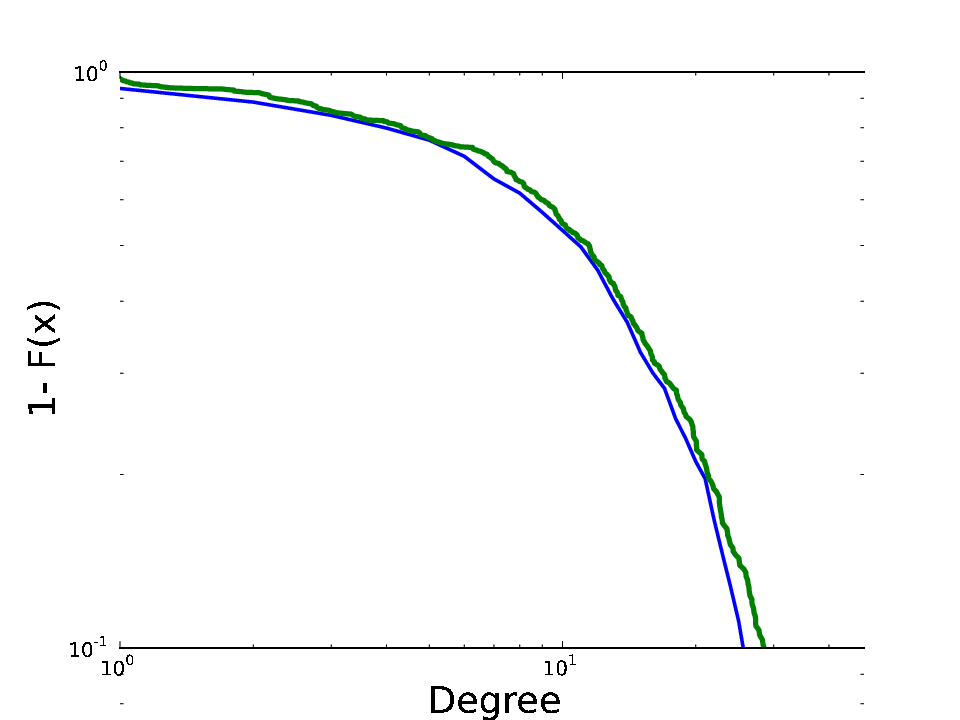

We use two real social networks, namely two Facebook subnetworks comprising 503 () graduate and 1220 () undergraduate students, respectively [20]. We also generate three synthetic networks, each possessing 1024 vertices, whose generative models frequently arise in practice in the analysis of networks. We generated a Barabasi-Albert Network [5] (), which is a preferential attachment model, a Network [10] () with , and a Power-Law Tree, whose node degree distribution follows a power-law distribution with exponent ().
First, we evaluate the performance of the algorithm to reconstruct the degree distribution of networks without inferring the network itself (Section 4.3). Figure 1 shows the reconstruction of the degree distribution using traces of the Barabasi-Albert Network and the two Facebook subnetworks. We used traces, and the plots show that the CCDF curves for the real degrees and for the reconstructed distribution have almost perfect overlap.
Turning our attention back to network inference, the lower-bound established in Section 3 tells us that the First-Edge algorithm is nearly optimal for perfect network inference in the general case. Thus, we assess the performance of our algorithms against this limit. The performance of First-Edge is notoriously predictable: if we use traces where is less than the total number of edges in the network, then it returns nearly edges which are all true positives, and it never returns false positives.
If we allow false positives, we can use heuristics to improve the First-Edge’s recall. To this end, we propose the following heuristic that uses the degree distribution reconstruction algorithm (Section 4.3) in a pre-processing phase, and places an edge in the inferred network provided the edge has probability at least of being in the graph. We call this heuristic First-Edge.


In First-Edge, we use the memoryless property of the exponential distribution to establish the probability of an edge pertaining to a network . The algorithm works as follows. Consider a node that appears as the root of a trace at time . When spreads the epidemic, some node is going to be the next infected at time , which was sampled from an exponential distribution with parameter . At time , notice that there are exactly nodes waiting to be infected by , and exactly waiting to be infected by , where and are the degrees of and respectively. At time any of these nodes is equally likely to be infected, due to the memoryless property. Moreover, the next node that appears in a trace after time is going to be infected by with probability and by with probability . We can approximate55 5 The exact probability depends on the number of edges between each of the nodes and the rest of the graph. this reasoning for larger prefixes of the trace: given a sequence of infected nodes starting at the source of the epidemic, the probability that is a neighbor of is roughly . Therefore, for every segment of a trace that starts at the source, we infer an edge if , computed using the reconstructed degrees, where is a tunable parameter. In our experiments we arbitrarily chose .
Note that First-Edge+ may not terminate as soon as we have inferred enough edges, even in the event that all true positives have been found, an effect that degrades its precision performance. To prevent this, we keep a variable , which can be thought of as the temperature of the inference process. Let be a counter of the edges inferred at any given time during the inference process, and be an estimate of the total number of edges, computed using the degree reconstruction algorithm in the pre-processing phase. We define and run the algorithm as long as . In addition, whenever we infer a new edge, we flip a coin and remove, with probability , a previously inferred edge with the lowest estimated probability of existence. Thus, while the network is “cold”, i.e., many undiscovered edges, edges are rapidly added and a few are removed, which boosts the recall. When the network is “warm”, i.e., the number of inferred edges approaches , we carefully select edges by exchanging previously inferred ones with better choices, thereby contributing to the precision.
Figure 2 contrasts the performance of First-Edge, First-Edge and an existing network algorithm, NetInf [15], with respect to the F1 measure. NetInf requires the number of edges in the network as input, and thus we give it an advantage, by setting the number of edges to the true cardinality of edges for each network.
In Figures 2(a) and 2(b), we observe that, as First-Edge and NetInf are less conservative, their F1 performances have an advantage over First-Edge for small numbers of traces, with First-Edge+ approaching the performance to NetInf. Interestingly, in Figure 2(c), we see that First-Edge and First-Edge+ achieve perfect tree inference with roughly traces, which reflects a trace complexity in rather than in , which is the trace complexity of Algorithm 1.66 6 In our experiments Algorithm 1 consistently returned the true edge set without false positives with traces for various networks of various sizes. Therefore, in the interest of space we omit the data from these experiments. This result illustrates the relevance of the algorithms for special cases we developed in Section 5. Last, we observe that random graphs seem to have very large trace complexity. This is shown in Figure 2(d), where neither our algorithms nor NetInf can achieve high inference performance, even for large numbers of traces.
In accordance with our discussion in Section 4.1, we confirm that, in practice, we need significantly fewer than traces for inferring most of the edges. It is perhaps surprising that First-Edge+, which is extremely simple, achieves comparable performance to the more elaborate counterpart, NetInf. In addition, while NetInf reaches a plateau that limits its performance, First-Edge+ approaches perfect inference as the number of traces goes to . In the cases in which NetInf achieves higher performance than First-Edge+, the latter is never much worse than the former. This presents a practitioner with a trade-off between the two algorithms. For large networks, while First-Edge+ is extremely easy to implement and makes network inferences (in a preemptive fashion) in a matter of seconds, NetInf takes a couple of hours to run to completion and requires the implementation of an elaborate algorithm.
7 Conclusion
Our goal is to provide the building blocks for a rigorous foundation to the rapidly-expanding network inference topic. Previous works have validated claims through experiments on relatively small graphs as compared to the large number of traces utilized, whereas the relation that binds these two quantities remains insufficiently understood. Accordingly, we believe that a solid foundation for the network inference problem remains a fundamental open question, and that works like [23], as well as ours, provide the initial contributions toward that goal.
Our results have direct applicability in the design of network inference algorithms. More specifically, we rigorously study how much useful information can be extracted from a trace for network inference, or more generally, the inference of network properties without reconstructing the network, such as the node degree distribution. We first show that, to perfectly reconstruct general graphs, nothing better than looking at the first pair of infected nodes in a trace can really be done. We additionally show that the remainder of a trace contains rich information that can reduce the trace complexity of the task for special case graphs. Finally, we build on the previous results to develop extremely simple and efficient reconstruction algorithms that exhibit competitive inference performance with the more elaborate and computationally costly ones.
Some open technical questions stemming from our work are immediately apparent. For instance, what is the true lower bound for perfect reconstruction? Is it , or some other bound which, in the case of the clique, reduces to what we have shown? And, are there other meaningful statistics apart from the degree distribution that can be efficiently recovered? For graphs with maximum degree , our perfect reconstruction algorithm has running time exponential in : is this exponential dependence necessary? And while the algorithm’s trace complexity is polynomial in , the upper bound of proven here is far from matching the lower bound ; what is the correct dependence of trace complexity on ? The bounded-degree restriction, while natural, is unlikely to be satisfied by real-world networks; is perfect reconstruction possible for the types of graphs that are likely to occur in real-world situations?
Perhaps the most relevant avenue for future research in our context is to go beyond the notion of perfect reconstruction. This notion, while quite reasonable as a first step, is not flexible enough to be deployed in practical situations. One would need to take into account the possibility of accepting some noise, i.e. some false positives as well as false negatives. So the main issue is to look for algorithms and lower bounds that are expressed as a function of the precision and recall one is willing to accept in an approximate reconstruction algorithm.
Finally, it would be very interesting to develop similar results, or perhaps even a theory, of trace complexity for other types of information spreading dynamics.
Appendix A Proofs missing from Section 4.2
We start by proving Lemma 4.2, which is the combinatorial heart of our lower bound.
Proof of Lemma 4.2.
Points 1, 2, 4 are either obvious or simple consequences of point 3, which we now consider. For , let be the probability that appear (in any order) in the positions conditioned on the starting node being different from . Moreover, let the probability that appear (in any order) in the positions conditioned on the starting node being one of . Then , for , and .
We now compute . First, we assume . Them
Now assume that . We have:
By telescoping, specifically by , we can simplify the expression to:
Moreover, by trying to simplify the product term, and by collecting the binomial, we get:
Then, observe that for each , , (and, if , ) we have:
We highlight the product inside ’s expression:
We take the product of the denominators of the ratios, obtaining:
Therefore, we have
We now turn back to expressions. Plugging in our approximation of , we get:
The term is bounded within and . Therefore, if , (and if , ), we have:
∎
Before moving on the two main Lemmas, we state (a corollary of) the Berry-Esseen Theorem [6, 11] which will be a crucial part of their proofs.
Theorem A.1 (Berry-Esseen [6, 11]).
Let be independent random variables, such that for each , and such that is finite. Then, if we let and , we have that
and
Proof of Lemma 4.3.
Let be the number of traces having one of the nodes in in position , and the other in position . Then, . We start by computing the likelihoods of assuming that the unknown graph is, respectively, or . We proved in Lemma 4.2, that the two likelihood of a trace only depends on the positions of and . Therefore, if is the probability of obtaining a trace with -positions equal to in the graph , we have:
Regardless of the unknown graph, we have that the probability that there exists for which there exists at least one such that is at most . We condition on the opposite event. Then,
where be the function defined in the statement of Lemma 4.2.
We aim to prove that the random variable is sufficiently anti-concentrated that, for any unknown graph , the probability that and . This will prove that one cannot guess what is the unknown graph with probability more than .
First, let and be two random variable having support , the first uniform and the second distributed like the distribution of Lemma 4.2.
We will compute a number of expectations so to finally apply Berry-Esseen theorem. First, recall that . Therefore,
Moreover,
Recall that . Then
Therefore, . Moreover,
It follows that, for , we have
We now move to the second moments. First observe that, for ,
We lower bound both and with
Analogously, we have that and can both be upper bounded by
We then have, for ,
Moreover, the variance of , , is equal to .
By linearity of expectation, regardless of the unknown graph, if we let , we have that
We upper bound both and with
It follows that
Now, we apply the Berry-Esseen bound with and . We compute the error term of the Berry-Esseen theorem:
Therefore, will behave approximately like a gaussian in a radius of (at least) standard deviations around its mean. Observe that the standard deviation satisfies . Since (by ), we have . Therefore, regardless of the unknown graph, the probability that will be positive is .∎
We finally prove Lemma 4.4, which deals with the likelihoods of the waiting times in the traces.
Proof of Lemma 4.4.
Let and be two exponential density functions with parameters and . Since we will be considering ratio of likelihoods, we compute the ratio of the two densities:
Observe that, if , it holds that
| (11) |
Let if, in the th trace, exactly one of the nodes in was within the first informed nodes; otherwise, let . Then .
For and , let be the time waited (from the last time a node was informed) to inform the th node in the th of the traces having exactly one of the two nodes in the first positions. By the memoryless property of the exponential random variables, and by the fact that the minimum of iid random variables is distributed like , we have that (once we condition on the ’s) the ’s variables are independent, and that is distributed like where is the size of the cut induced by the first nodes of the th trace (of those having one of the nodes within the first nodes). Further, from the scaling property of the exponential random variables, we have that is distributed like .
Let . Let be the random variable conditioned on , and let be the random variable conditioned on (observe that, since is conditioned on , both and will also be conditioned on ). Then,
Now, let be distributed like , for some . In general, we have . If we let , we obtain . Moreover, we have
We also have,
where the inequality follows from .
Let us consider , . They are the sum, over , of independent exponential random variables with parameters . If we center each of those variables in (that is, we remove the expected value of each exponential variable), obtaining — say — variables , we can write as:
Let us bound the absolute difference between the expected values of and , recalling that , for each :
We now aim to show that , for both and . To do so, we use the Berry-Esseen theorem (Theorem A.1). We apply it to our collection of variables (which will play the variables’ role in the Berry-Esseen theorem). We get:
and
Therefore,
and
Therefore, . We set . Then, for each , the probability that exceeds by at least is at least .
Now consider, the likelihoods , of the sequence of waiting times with each of the two graphs. We have:
Then,
Since , we can apply Equation (11), and the former product equals
The former product simplifies to . Therefore,
Therefore, if , and if . We have that ; moreover, the probability that the difference between and its expectation is at least , and the probability that it is at most , are both , since the standard deviation satisfies .
Therefore, the probability that the likelihood of graph is higher than the likelihood of graph is , regardless of whether the unknown graph was or . The proof is concluded. ∎
References
- [1] B. Abrahao, F. Chierichetti, R. Kleinberg, and A. Panconesi. Trace complexity of network inference. In Proc. of the 19th ACM SIGKDD Int’l Conf. on Knowledge Discovery and Data Mining, 2013.
- [2] E. Adar and L. A. Adamic. Tracking information epidemics in blogspace. In Proc. of the 2005 IEEE/WIC/ACM Int’l Conf. on Web Intelligence, 2005.
- [3] N. Bailey. The Mathematical Theory of Infectious Diseases and its Applications. Griffin, London, 1975.
- [4] E. Bakshy, J. M. Hofman, W. A. Mason, and D. J. Watts. Everyone’s an influencer: quantifying influence on twitter. In Proc. of the 4th ACM Int’l Conf. on Web search and Data Mining, 2011.
- [5] A.-L. Barabási and R. Albert. Emergence of Scaling in Random Networks. Science, 286(5439):509–512, Oct. 1999.
- [6] A. C. Berry. The accuracy of the Gaussian approximation to the sum of independent variates. Transactions of the American Mathematical Society, 49:122–136, 1941.
- [7] S. G. Bobkov and M. Ledoux. On modified logarithmic sobolev inequalities for bernoulli and poisson measures. Journal of Functional Analysis, 156(2):347 – 365, 1998.
- [8] N. DU, L. Song, A. Smola, and M. Yuan. Learning networks of heterogeneous influence. In Advances in Neural Information Processing Systems 25, pages 2789–2797. 2012.
- [9] R. Durrett. Probability: Theory and examples. Cambridge Series in Statistical and Probabilistic Mathematics, 2011.
- [10] P. Erdös and A. Rényi. On the evolution of random graphs. In Pub. of the Mathematical Institute of the Hungarian Academy of Sciences, pages 17–61, 1960.
- [11] C.-G. Esseen. A moment inequality with an application to the central limit theorem. Skand. Aktuarietidskr., 39:160–170, 1956.
- [12] M. Faloutsos, P. Faloutsos, and C. Faloutsos. On power-law relationships of the internet topology. SIGCOMM Comput. Commun. Rev., 29(4):251–262, Aug. 1999.
- [13] T. Gneiting and A. E. Raftery. Strictly proper scoring rules, prediction, and estimation. J. Amer. Stat. Assoc., 102:359–378, 2007.
- [14] M. Gomez-Rodriguez, D. Balduzzi, and B. Schölkopf. Uncovering the temporal dynamics of diffusion networks. In Proc. of the 28th Int’l Conf. on Machine Learning, 2011.
- [15] M. Gomez-Rodriguez, J. Leskovec, and A. Krause. Inferring networks of diffusion and influence. In Proc. of the 16th ACM SIGKDD Int’l Conf. on Knowledge Discovery and Data Mining, 2010.
- [16] V. Gripon and M. Rabbat. Reconstructing a graph from path traces. CoRR, abs/1301.6916, 2013.
- [17] D. Gruhl, R. Guha, D. Liben-Nowell, and A. Tomkins. Information diffusion through blogspace. In Proc. of the 13th Int’l Conf. on World Wide Web, 2004.
- [18] D. Kempe, J. Kleinberg, and E. Tardos. Maximizing the spread of influence through a social network. In Proc. of the 9th ACM SIGKDD Int’l Conf. on Knowledge Discovery and Data Mining, 2003.
- [19] I. Kontoyiannis and M. Madiman. Measure concentration for compound poisson distributions. Electron. Commun. Probab., 11:no. 5, 45–57, 2006.
- [20] A. Mislove, B. Viswanath, K. Gummadi, and P. Druschel. You are who you know: Inferring user profiles in online social networks. In Proc. 3rd ACM Int’l. Conf. on Web Search and Data Mining, 2010.
- [21] R. Motwani and P. Rahgavan. Randomized Algorithms. Cambridge University Press, 1995.
- [22] S. Myers and J. Leskovec. On the convexity of latent social network inference. In Advances in Neural Information Processing Systems 23, pages 1741–1749. 2010.
- [23] P. Netrapalli and S. Sanghavi. Learning the graph of epidemic cascades. In SIGMETRICS, pages 211–222, 2012.
- [24] M. E. J. Newman. The structure and function of complex networks. SIAM REVIEW, 45:167–256, 2003.
- [25] E. M. Rogers and E. Rogers. Diffusion of Innovations. Free Press, 5th edition, Aug. 2003.